ADP-12-16/T783

Threshold Corrections in the Exceptional Supersymmetric Standard Model

Peter Athron, Dominik Stöckinger, Alexander Voigt

ARC Centre of Excellence for Particle Physics at the Terascale, School of Chemistry and Physics, University of Adelaide, Adelaide, SA 5005, Australia
Institut für Kern und Teilchenphysik, TU Dresden, Dresden, D-01062, Germany.

We calculate threshold corrections to the running gauge and Yukawa couplings in the Exceptional Supersymmetric Standard Model (E6SSM) and analyse the more precise and reliable mass spectra in a constrained model (CE6SSM). Full expressions for the corrections are provided and the implementation into a spectrum generator is described. We find a dramatic reduction in the matching scale dependency of the masses of many states and observe a significant adjustment of the correlation of low-scale physical masses and high-scale parameters. Still, in substantial regions of parameter space the mass of the lightest Higgs is compatible with the new boson discovered at the LHC and the model satisfies limits from collider searches for squark, gluinos and Zsuperscript𝑍Z^{\prime} bosons. We study the implications for gauge coupling unification from a new dependency of the spectrum on so-called survival Higgs fields which cannot be addressed without the inclusion of the threshold corrections.

1 Introduction

Supersymmetric (SUSY) extensions of the Standard Model (SM) with TeV-scale SUSY breaking provide very attractive models for new physics which could be discovered at the Large Hadron Collider (LHC). Such models can solve the hierarchy problem of the SM due to the cancellation of quadratic divergences, enable embedding into Grand Unified Theories (GUTs), and thereby provide an explanation of the U(1)Y𝑈subscript1𝑌U(1)_{Y} rational charges, postulated ad hoc in the SM. These fundamental motivations do not imply any minimality condition on the particle content or gauge structure.

Here we consider the Exceptional Supersymmetric Standard Model111For a brief review see [1]. (E6SSM) [2, 3], which is a non-minimal SUSY extension of the SM with an extra U(1)N𝑈subscript1𝑁U(1)_{N} gauge symmetry and new exotic matter at the TeV scale. A new Higgs singlet together with an extra U(1)𝑈1U(1) gauge symmetry solve the well-known μ𝜇\mu-problem [4] of the Minimal Supersymmetric Standard Model (MSSM) without introducing the tadpole or domain wall problems of the Next-to-MSSM222Reviews are given in [5]. [6]. These features also allow the lightest Higgs boson to be substantially heavier than in the MSSM or NMSSM already at tree-level, through new U(1)N𝑈subscript1𝑁U(1)_{N} D𝐷D-term contributions and an additional F𝐹F-term contribution from the superpotential coupling between the singlet and doublet Higgs bosons, which can be substantially larger than the parallel NMSSM term due to different perturbative limits on the coupling [3].

The model is inspired and motivated by E6subscript𝐸6E_{6} GUTs, as the extra U(1)𝑈1U(1) appears from the breakdown of E6subscript𝐸6E_{6} and the exotic new matter comes from complete E6subscript𝐸6E_{6} multiplets surviving to low energies, ensuring the cancellation of gauge anomalies. The extra U(1)𝑈1U(1) gauge group of the E6SSM is uniquely chosen such that right-handed neutrinos are neutral, allowing large Majorana masses and a high-scale see-saw mechanism.

The E6subscript𝐸6E_{6} symmetry itself can arise from E8×E8subscript𝐸8subscriptsuperscript𝐸8E_{8}\times E^{\prime}_{8} Heterotic string theory after the breakdown of E8subscript𝐸8E_{8} [7]. The E8subscriptsuperscript𝐸8E^{\prime}_{8} then plays the role of a hidden sector interacting with the visible sector only through gravitational interactions and leads to TeV-scale SUSY breaking, generating a set of soft SUSY-breaking parameters.

In recent publications [8, 9] a constrained version (CE6SSM) was introduced where all the soft SUSY-breaking masses are determined by a universal scalar mass, m0subscript𝑚0m_{0}, gaugino mass M1/2subscript𝑀12M_{1/2} and soft trilinear scalar coupling A𝐴A. Owing to the unification of matter and Higgs fields in complete GUT multiplets the CE6SSM is particularly well motivated. In Refs. [8, 9] the low-energy mass spectra were explored for the first time with benchmark scenarios, representing the phenomenologically distinct possibilities in the model. This work has recently been updated to look at spectra which are consistent with the 125125125 GeV Higgs signal and recent searches for squarks and gluinos [10]. Other aspects of this model and similar variants have also been discussed in Refs. [11, 12, 13, 14, 15, 16, 17, 18, 19, 20, 21].

The calculations in Refs. [8, 9, 10] neglect important threshold corrections and involve a significant dependence on unphysical threshold scales. This limits the accuracy of phenomenological results and it was stated that the precision for the masses was not better than 10%percent1010\%.

However to facilitate model discrimination from data, and ultimately to reconstruct parameters in the event of a signal, precise predictions of the TeV scale SUSY masses predicted from GUT scale parameters are important. Indeed for the MSSM there are already a number of state of the art spectrum generators publicly available [22, 23, 24, 25, 26] which calculate the spectrum for scenarios, such as the constrained MSSM (CMSSM). Typically these employ two-loop renormalization group equations, full one-loop matching conditions for gauge and Yukawa couplings and one-loop shifts to pole masses and comparisons of their predicted masses suggests an accuracy of about 1%percent11\% [27].

The present paper is devoted to the calculation of threshold corrections to the running gauge and Yukawa couplings in the Exceptional Supersymmetric Standard Model (E6SSM), which enable a more precise evaluation of the mass spectrum from high-scale assumptions, and to an extensive study of the phenomenological consequences in the CE6SSM. As in Refs. [8, 9, 10] we employ two-loop renormalization group equations for the running of the gauge and Yukawa couplings between the weak scale and the GUT scale. As a major improvement, we also compute and take into account the corresponding one-loop threshold corrections arising in the transition from the full CE6SSM to the SM as a low-energy effective theory. We show that the individual threshold corrections indeed drastically reduce the dependence of our results on the unphysical threshold scale. The resulting, more accurate and reliable mass spectra are discussed. Particular attention is paid to the prediction for the Higgs mass and the gluino mass. We confirm the recent result of Ref. [10] that the lightest Higgs mass can easily be in agreement with recent LHC discovery of a new boson [28, 29]. Finally we use our improved precision to study gauge coupling unification333Previous studies [30, 31] used trivial matching conditions, equivalent to assuming all new E6SSM states and all new MSSM states have common masses, TE6SSMsubscript𝑇E6SSMT_{\text{E${}_{6}$SSM}} and TMSSMsubscript𝑇MSSMT_{\text{MSSM}} respectively. Such scenarios are clearly not realised in the constrained version of the model. for the CE6SSM and the impact of the survival Higgs sector, which appears only via threshold corrections.

This paper is structured as follows. In Sec. 2 we briefly outline the E6SSM model, in Sec. 3 we describe the improved spectrum calculations, give analytical results for the threshold corrections. Sec. 4 describes the application to an improved CE6SSM spectrum generator and explains the full numerical procedure used. In Sec. 5 we illustrate the effect of the thresholds and the improvement in accuracy of our results, and we give an extensive discussion of the resulting model predictions.

2 The E6SSM

The E6SSM is a supersymmetric gauge theory, inspired by E6subscript𝐸6E_{6} GUTs in which the E6subscript𝐸6E_{6} is broken at the GUT scale MXsubscript𝑀𝑋M_{X} via the Hosotani mechanism [32] down to the low-energy gauge group of the E6SSM,

SU(3)c×SU(2)L×U(1)Y×U(1)N.𝑆𝑈subscript3c𝑆𝑈subscript2L𝑈subscript1𝑌𝑈subscript1𝑁\displaystyle SU(3)_{\text{c}}\times SU(2)_{\text{L}}\times U(1)_{Y}\times U(1)_{N}. (1)

Here the U(1)N𝑈subscript1𝑁U(1)_{N} is a special case of a U(1)𝑈superscript1U(1)^{\prime} symmetry arising from E6subscript𝐸6E_{6} breaking,

U(1)=U(1)χcosθ+U(1)ψsinθ,𝑈superscript1𝑈subscript1𝜒𝜃𝑈subscript1𝜓𝜃\displaystyle U(1)^{\prime}=U(1)_{\chi}\cos\theta+U(1)_{\psi}\sin\theta, (2)

with tanθ=15𝜃15\tan\theta=\sqrt{15}, where the gauge groups U(1)χ𝑈subscript1𝜒U(1)_{\chi} and U(1)ψ𝑈subscript1𝜓U(1)_{\psi} are defined by the breaking of E6SO(10)×U(1)ψsubscript𝐸6𝑆𝑂10𝑈subscript1𝜓E_{6}\rightarrow SO(10)\times U(1)_{\psi} and SO(10)SU(5)×U(1)χ𝑆𝑂10𝑆𝑈5𝑈subscript1𝜒SO(10)\rightarrow SU(5)\times U(1)_{\chi} [33, 34].

The choice of U(1)N𝑈subscript1𝑁U(1)_{N} makes the right-handed neutrino a pure gauge singlet, thus allowing a gauge invariant Majorana mass term enabling a high-scale seesaw mechanism for the generation of neutrino masses. All other matter from complete E6subscript𝐸6E_{6} matter multiplets survives to low energies, thereby ensuring the cancellation of gauge anomalies.

The three families of E6SSM  matter particles fill complete (𝟐𝟕)isubscript27𝑖(\mathbf{27})_{i} representations of the E6subscript𝐸6E_{6} group, ensuring that full low energy gauge group, including the new U(1)N𝑈subscript1𝑁U(1)_{N} gauge symmetry, is anomaly free. In addition to these, the model has two Higgs-like doublets H^superscript^𝐻\hat{H}^{\prime} and barH^^barsuperscript𝐻\hat{\mathrm{bar}{H^{\prime}}}, the so-called survival Higgs doublets, both originating from extra (𝟐𝟕)superscript27(\mathbf{27})^{\prime} and (𝟐𝟕¯)superscript¯27(\mathbf{\overline{27}})^{\prime} representations to ensure gauge coupling unification at a high scale MXsubscript𝑀𝑋M_{X}. The decomposition of the fundamental (𝟐𝟕)27(\mathbf{27}) representation under SU(5)×U(1)N𝑆𝑈5𝑈subscript1𝑁SU(5)\times U(1)_{N} and (1) is listed in Tab. 1.

Field GSM×U(1)Nsubscript𝐺SM𝑈subscript1𝑁G_{\text{SM}}\times U(1)_{N} SU(5)×U(1)N𝑆𝑈5𝑈subscript1𝑁SU(5)\times U(1)_{N} E6subscript𝐸6E_{6}
Q^i=(Q^uiQ^di)subscript^𝑄𝑖subscript^𝑄subscript𝑢𝑖subscript^𝑄subscript𝑑𝑖\hat{Q}_{i}=(\hat{Q}_{u_{i}}\ \ \hat{Q}_{d_{i}}) (𝟑,𝟐,16,1)isubscript32161𝑖(\mathbf{3},\mathbf{2},{\textstyle\frac{1}{6}},1)_{i} }casesmissing-subexpressionmissing-subexpression\left.\begin{array}[]{c}\\ \\ \\ \end{array}\right\} (𝟏𝟎,1)isubscript101𝑖(\mathbf{10},1)_{i} }casesmissing-subexpressionmissing-subexpressionmissing-subexpressionmissing-subexpressionmissing-subexpressionmissing-subexpressionmissing-subexpressionmissing-subexpressionmissing-subexpressionmissing-subexpression\left.\begin{array}[]{c}\\ \\ \\ \\ \\ \\ \\ \\ \\ \\ \\ \end{array}\right\} (𝟐𝟕)isubscript27𝑖(\mathbf{27})_{i}
u^iCsuperscriptsubscript^𝑢𝑖𝐶\hat{u}_{i}^{C} (bar𝟑,𝟏,23,1)isubscriptbar31231𝑖(\mathbf{\mathrm{bar}{3}},\mathbf{1},{\textstyle-\frac{2}{3}},1)_{i}
e^iCsuperscriptsubscript^𝑒𝑖𝐶\hat{e}_{i}^{C} (𝟏,𝟏,1,1)isubscript1111𝑖(\mathbf{1},\mathbf{1},1,1)_{i}
d^iCsuperscriptsubscript^𝑑𝑖𝐶\hat{d}_{i}^{C} (bar𝟑,𝟏,13,2)isubscriptbar31132𝑖(\mathbf{\mathrm{bar}{3}},\mathbf{1},{\textstyle\frac{1}{3}},2)_{i} }casesmissing-subexpression\left.\begin{array}[]{c}\\ \\ \end{array}\right\} (bar𝟓,2)isubscriptbar52𝑖(\mathbf{\mathrm{bar}{5}},2)_{i}
L^i=(L^νiL^ei)subscript^𝐿𝑖subscript^𝐿subscript𝜈𝑖subscript^𝐿subscript𝑒𝑖\hat{L}_{i}=(\hat{L}_{\nu_{i}}\ \ \hat{L}_{e_{i}}) (𝟏,𝟐,12,2)isubscript12122𝑖(\mathbf{1},\mathbf{2},{\textstyle-\frac{1}{2}},2)_{i}
barD^isubscript^bar𝐷𝑖\hat{\mathrm{bar}{D}}_{i} (bar𝟑,𝟏,13,3)isubscriptbar31133𝑖(\mathbf{\mathrm{bar}{3}},\mathbf{1},{\textstyle\frac{1}{3}},-3)_{i} }casesmissing-subexpression\left.\begin{array}[]{c}\\ \\ \end{array}\right\} (bar𝟓,3)isubscriptbar53𝑖(\mathbf{\mathrm{bar}{5}},-3)_{i}
H^1i=(H^1i0H^1i)subscript^𝐻1𝑖subscriptsuperscript^𝐻01𝑖subscriptsuperscript^𝐻1𝑖\hat{H}_{1i}=(\hat{H}^{0}_{1i}\ \ \hat{H}^{-}_{1i}) (𝟏,𝟐,12,3)isubscript12123𝑖(\mathbf{1},\mathbf{2},{\textstyle-\frac{1}{2}},-3)_{i}
D^isubscript^𝐷𝑖\hat{D}_{i} (𝟑,𝟏,13,2)isubscript31132𝑖(\mathbf{3},\mathbf{1},{\textstyle-\frac{1}{3}},-2)_{i} }casesmissing-subexpression\left.\begin{array}[]{c}\\ \\ \end{array}\right\} (𝟓,2)isubscript52𝑖(\mathbf{5},-2)_{i}
H^2i=(H^2i+H^2i0)subscript^𝐻2𝑖subscriptsuperscript^𝐻2𝑖subscriptsuperscript^𝐻02𝑖\hat{H}_{2i}=(\hat{H}^{+}_{2i}\ \ \hat{H}^{0}_{2i}) (𝟏,𝟐,12,2)isubscript12122𝑖(\mathbf{1},\mathbf{2},{\textstyle\frac{1}{2}},-2)_{i}
S^isubscript^𝑆𝑖\hat{S}_{i} (𝟏,𝟏,0,5)isubscript1105𝑖(\mathbf{1},\mathbf{1},0,5)_{i} (𝟏,5)isubscript15𝑖(\mathbf{1},5)_{i}
N^iCsuperscriptsubscript^𝑁𝑖𝐶\hat{N}_{i}^{C} (𝟏,𝟏,0,0)isubscript1100𝑖(\mathbf{1},\mathbf{1},0,0)_{i} (𝟏,0)isubscript10𝑖(\mathbf{1},0)_{i}
H^=(H^0H^)superscript^𝐻superscript^superscript𝐻0superscript^superscript𝐻\hat{H}^{\prime}=(\hat{H^{\prime}}^{0}\ \ \hat{H^{\prime}}^{-}) (𝟏,𝟐,12,2)12122(\mathbf{1},\mathbf{2},{\textstyle-\frac{1}{2}},2) (bar𝟓,2)superscriptbar52absent\ni(\mathbf{\mathrm{bar}{5}},2)^{\prime} (𝟐𝟕)superscript27absent\ni(\mathbf{27})^{\prime}
barH^=(barH^+barH^0)^barsuperscript𝐻superscript^barsuperscript𝐻superscript^barsuperscript𝐻0\hat{\mathrm{bar}{H^{\prime}}}=({\hat{\mathrm{bar}{H^{\prime}}}}^{+}\ \ {\hat{\mathrm{bar}{H^{\prime}}}}^{0}) (𝟏,𝟐,12,2)12122(\mathbf{1},\mathbf{2},{\textstyle\frac{1}{2}},-2) (𝟓,2)superscript52absent\ni(\mathbf{5},-2)^{\prime} (𝟐𝟕¯)superscript¯27absent\ni(\mathbf{\overline{27}})^{\prime}
V^gasubscriptsuperscript^𝑉𝑎𝑔\hat{V}^{a}_{g} (𝟖,𝟏,0,0)8100(\mathbf{8},\mathbf{1},0,0) (𝟐𝟒,0)240absent\ni(\mathbf{24},0) (𝟕𝟖)78absent\ni(\mathbf{78})
V^Wisuperscriptsubscript^𝑉𝑊𝑖\hat{V}_{W}^{i} (𝟏,𝟑,0,0)1300(\mathbf{1},\mathbf{3},0,0) (𝟐𝟒,0)240absent\ni(\mathbf{24},0) (𝟕𝟖)78absent\ni(\mathbf{78})
V^Ysubscript^𝑉𝑌\hat{V}_{Y} (𝟏,𝟏,0,0)1100(\mathbf{1},\mathbf{1},0,0) (𝟐𝟒,0)240absent\ni(\mathbf{24},0) (𝟕𝟖)78absent\ni(\mathbf{78})
V^Nsubscript^𝑉𝑁\hat{V}_{N} (𝟏,𝟏,0,0)1100(\mathbf{1},\mathbf{1},0,0) (𝟏,0)10absent\ni(\mathbf{1},0) (𝟕𝟖)78absent\ni(\mathbf{78})
Tab. 1: E6SSM SUSY multiplets and their gauge quantum numbers (generation index i=1,2,3𝑖123i=1,2,3), where GSMSU(3)c×SU(2)L×U(1)Ysubscript𝐺SM𝑆𝑈subscript3c𝑆𝑈subscript2L𝑈subscript1𝑌G_{\text{SM}}\equiv SU(3)_{\text{c}}\times SU(2)_{\text{L}}\times U(1)_{Y}. For the abelian groups U(1)Y𝑈subscript1𝑌U(1)_{Y} and U(1)N𝑈subscript1𝑁U(1)_{N} the charges Y/2𝑌2Y/2 and N/2𝑁2N/2 are listed.
Superfield Component fields
Spin 00 Spin 1/2121/2 Spin 111
Q^i=(Q^uiQ^di)Tsubscript^𝑄𝑖superscriptsubscript^𝑄subscript𝑢𝑖subscript^𝑄subscript𝑑𝑖𝑇\hat{Q}_{i}=(\hat{Q}_{u_{i}}\ \ \hat{Q}_{d_{i}})^{T} q~iL=(u~iLd~iL)Tsubscript~𝑞𝑖𝐿superscriptsubscript~𝑢𝑖𝐿subscript~𝑑𝑖𝐿𝑇\tilde{q}_{iL}=(\tilde{u}_{iL}\ \ \tilde{d}_{iL})^{T} qiL=(uiLdiL)Tsubscript𝑞𝑖𝐿superscriptsubscript𝑢𝑖𝐿subscript𝑑𝑖𝐿𝑇q_{iL}=(u_{iL}\ \ d_{iL})^{T}
u^iCsubscriptsuperscript^𝑢𝐶𝑖\hat{u}^{C}_{i} u~iRsubscriptsuperscript~𝑢𝑖𝑅\tilde{u}^{*}_{iR} uiRCsubscriptsuperscript𝑢𝐶𝑖𝑅u^{C}_{iR}
d^iCsubscriptsuperscript^𝑑𝐶𝑖\hat{d}^{C}_{i} d~iRsubscriptsuperscript~𝑑𝑖𝑅\tilde{d}^{*}_{iR} diRCsubscriptsuperscript𝑑𝐶𝑖𝑅d^{C}_{iR}
L^i=(L^νiL^ei)Tsubscript^𝐿𝑖superscriptsubscript^𝐿subscript𝜈𝑖subscript^𝐿subscript𝑒𝑖𝑇\hat{L}_{i}=(\hat{L}_{\nu_{i}}\ \ \hat{L}_{e_{i}})^{T} ~iL=(ν~iLe~iL)Tsubscript~𝑖𝐿superscriptsubscript~𝜈𝑖𝐿subscript~𝑒𝑖𝐿𝑇\tilde{\ell}_{iL}=(\tilde{\nu}_{iL}\ \ \tilde{e}_{iL})^{T} iL=(νiLeiL)Tsubscript𝑖𝐿superscriptsubscript𝜈𝑖𝐿subscript𝑒𝑖𝐿𝑇\ell_{iL}=(\nu_{iL}\ \ e_{iL})^{T}
e^iCsubscriptsuperscript^𝑒𝐶𝑖\hat{e}^{C}_{i} e~iRsubscriptsuperscript~𝑒𝑖𝑅\tilde{e}^{*}_{iR} eiRCsubscriptsuperscript𝑒𝐶𝑖𝑅e^{C}_{iR}
N^iCsubscriptsuperscript^𝑁𝐶𝑖\hat{N}^{C}_{i} ν~iRsubscriptsuperscript~𝜈𝑖𝑅\tilde{\nu}^{*}_{iR} νiRCsubscriptsuperscript𝜈𝐶𝑖𝑅\nu^{C}_{iR}
D^isubscript^𝐷𝑖\hat{D}_{i} D~iLsubscript~𝐷𝑖𝐿\tilde{D}_{iL} DiLsubscript𝐷𝑖𝐿D_{iL}
barD^isubscript^bar𝐷𝑖\hat{\mathrm{bar}{D}}_{i} D~iRsubscriptsuperscript~𝐷𝑖𝑅\tilde{D}^{*}_{iR} DiRCsuperscriptsubscript𝐷𝑖𝑅𝐶D_{iR}^{C}
H^1i=(H^1i0H^1i)Tsubscript^𝐻1𝑖superscriptsubscriptsuperscript^𝐻01𝑖subscriptsuperscript^𝐻1𝑖𝑇\hat{H}_{1i}=(\hat{H}^{0}_{1i}\ \ \hat{H}^{-}_{1i})^{T} H1i=(H1i0H1i)Tsubscript𝐻1𝑖superscriptsubscriptsuperscript𝐻01𝑖subscriptsuperscript𝐻1𝑖𝑇H_{1i}=(H^{0}_{1i}\ \ H^{-}_{1i})^{T} H~1iL=(H~1iL0H~1iL)Tsubscript~𝐻1𝑖𝐿superscriptsubscriptsuperscript~𝐻01𝑖𝐿subscriptsuperscript~𝐻1𝑖𝐿𝑇\tilde{H}_{1iL}=(\tilde{H}^{0}_{1iL}\ \ \tilde{H}^{-}_{1iL})^{T}
H^2i=(H^2i+H^2i0)Tsubscript^𝐻2𝑖superscriptsubscriptsuperscript^𝐻2𝑖subscriptsuperscript^𝐻02𝑖𝑇\hat{H}_{2i}=(\hat{H}^{+}_{2i}\ \ \hat{H}^{0}_{2i})^{T} H2i=(H2i+H2i0)Tsubscript𝐻2𝑖superscriptsubscriptsuperscript𝐻2𝑖subscriptsuperscript𝐻02𝑖𝑇H_{2i}=(H^{+}_{2i}\ \ H^{0}_{2i})^{T} H~2iL=(H~2iL+H~2iL0)Tsubscript~𝐻2𝑖𝐿superscriptsubscriptsuperscript~𝐻2𝑖𝐿subscriptsuperscript~𝐻02𝑖𝐿𝑇\tilde{H}_{2iL}=(\tilde{H}^{+}_{2iL}\ \ \tilde{H}^{0}_{2iL})^{T}
S^isubscript^𝑆𝑖\hat{S}_{i} Sisubscript𝑆𝑖S_{i} S~isubscript~𝑆𝑖\tilde{S}_{i}
H^=(H^0H^)T^superscript𝐻superscriptsuperscript^superscript𝐻0superscript^superscript𝐻𝑇\hat{H^{\prime}}=({\hat{H^{\prime}}}^{0}\ \ {\hat{H^{\prime}}}^{-})^{T} H=(H0H)Tsuperscript𝐻superscriptsuperscriptsuperscript𝐻0superscriptsuperscript𝐻𝑇H^{\prime}=({H^{\prime}}^{0}\ \ {H^{\prime}}^{-})^{T} H~L=(H~L0H~L)Tsubscript~superscript𝐻𝐿superscriptsubscriptsuperscript~superscript𝐻0𝐿subscriptsuperscript~superscript𝐻𝐿𝑇\tilde{H^{\prime}}_{L}=(\tilde{H^{\prime}}^{0}_{L}\ \ \tilde{H^{\prime}}^{-}_{L})^{T}
barH^=(barH^+barH^0)T^barsuperscript𝐻superscriptsuperscript^barsuperscript𝐻superscript^barsuperscript𝐻0𝑇\hat{\mathrm{bar}{H^{\prime}}}=({\hat{\mathrm{bar}{H^{\prime}}}}^{+}\ \ {\hat{\mathrm{bar}{H^{\prime}}}}^{0})^{T} barH=(barH+barH0)Tbarsuperscript𝐻superscriptbarsuperscriptsuperscript𝐻barsuperscriptsuperscript𝐻0𝑇\mathrm{bar}{H^{\prime}}=({\mathrm{bar}{H^{\prime}}}^{+}\ \ {\mathrm{bar}{H^{\prime}}}^{0})^{T} barH~L=(barH~L+barH~L0)Tsubscript~barsuperscript𝐻𝐿superscriptsubscriptsuperscript~barsuperscript𝐻𝐿subscriptsuperscript~barsuperscript𝐻0𝐿𝑇\tilde{\mathrm{bar}{H^{\prime}}}_{L}=({\tilde{\mathrm{bar}{H^{\prime}}}}^{+}_{L}\ \ {\tilde{\mathrm{bar}{H^{\prime}}}}^{0}_{L})^{T}
V^gasubscriptsuperscript^𝑉𝑎𝑔\hat{V}^{a}_{g} g~asuperscript~𝑔𝑎\tilde{g}^{a} Gμasubscriptsuperscript𝐺𝑎𝜇G^{a}_{\mu}
V^Wisuperscriptsubscript^𝑉𝑊𝑖\hat{V}_{W}^{i} W~isuperscript~𝑊𝑖\tilde{W}^{i} Wμisuperscriptsubscript𝑊𝜇𝑖W_{\mu}^{i}
V^Ysubscript^𝑉𝑌\hat{V}_{Y} B~~𝐵\tilde{B} Bμsubscript𝐵𝜇B_{\mu}
V^Nsubscript^𝑉𝑁\hat{V}_{N} Z~superscript~𝑍\tilde{Z}^{\prime} Zμsubscriptsuperscript𝑍𝜇Z^{\prime}_{\mu}
Tab. 2: Component fields of the E6SSM superfields (generation index i=1,2,3𝑖123i=1,2,3). The charge conjugation of a spinor ψ𝜓\psi is defined as ψC:=CbarψTassignsuperscript𝜓𝐶𝐶barsuperscript𝜓𝑇\psi^{C}:=\operatorname{\mathnormal{C}}\mathrm{bar}{\psi}^{T}, where C=iγ2γ0𝐶𝑖superscript𝛾2superscript𝛾0\operatorname{\mathnormal{C}}=i\gamma^{2}\gamma^{0}.

All Standard Model fermions as well as their superpartners fit into the multiplets (𝟏𝟎,1)isubscript101𝑖(\mathbf{10},1)_{i} and (bar𝟓,2)isubscriptbar52𝑖(\mathbf{\mathrm{bar}{5}},2)_{i}. The (bar𝟓,3)bar53(\mathbf{\mathrm{bar}{5}},-3) and (𝟓,2)52(\mathbf{5},-2) representations contain Higgs-like doublets H^1isubscript^𝐻1𝑖\hat{H}_{1i}, H^2isubscript^𝐻2𝑖\hat{H}_{2i} and exotic colored matter fields D^isubscript^𝐷𝑖\hat{D}_{i}, barD^isubscript^bar𝐷𝑖\hat{\mathrm{bar}{D}}_{i}. The remaining SU(5)𝑆𝑈5SU(5) singlets (𝟏,0)isubscript10𝑖(\mathbf{1},0)_{i} and (𝟏,5)isubscript15𝑖(\mathbf{1},5)_{i} equate to right-handed neutrinos and fields S^isubscript^𝑆𝑖\hat{S}_{i}, respectively. A complete particle listing can be found in Tab. 2.

In an E6subscript𝐸6E_{6} GUT the gauge bosons and their superpartners fit into the adjoint (𝟕𝟖)78(\mathbf{78}) representation of the E6subscript𝐸6E_{6}, which is decomposed under the low-energy gauge group SU(3)c×SU(2)L×U(1)Y×U(1)N𝑆𝑈subscript3c𝑆𝑈subscript2L𝑈subscript1𝑌𝑈subscript1𝑁SU(3)_{\text{c}}\times SU(2)_{\text{L}}\times U(1)_{Y}\times U(1)_{N} into

(𝟕𝟖)78\displaystyle(\mathbf{78}) (𝟖,𝟏,0,0)+(𝟏,𝟑,0,0)+(𝟏,𝟏,0,0)+(𝟏,𝟏,0,0)+absent8100130011001100\displaystyle\rightarrow(\mathbf{8},\mathbf{1},0,0)+(\mathbf{1},\mathbf{3},0,0)+(\mathbf{1},\mathbf{1},0,0)+(\mathbf{1},\mathbf{1},0,0)+\dotsb (3)

The gluons present in a low-energy model are associated to (𝟖,𝟏,0,0)8100(\mathbf{8},\mathbf{1},0,0). The (𝟏,𝟑,0,0)1300(\mathbf{1},\mathbf{3},0,0) multiplet contains the weak gauge bosons and the two U(1)𝑈1U(1) gauge fields belong to the two (𝟏,𝟏,0,0)1100(\mathbf{1},\mathbf{1},0,0) representations. When the E6subscript𝐸6E_{6} is broken at the GUT scale MXsubscript𝑀𝑋M_{X}, the other gauge bosons are expected to have masses of the order of MXsubscript𝑀𝑋M_{X}. However, the E6SSM is a low-energy model by construction and does not include these heavy GUT gauge bosons.

As with the MSSM embedded into GUT models, the new bosons absent from the low-energy theory could give rise to significant threshold corrections to gauge coupling unification at MXsubscript𝑀𝑋M_{X}. This should be borne in mind when studying the success or failure of gauge coupling unification within a low-energy SUSY model. However the purpose of this paper is to consider the low-energy threshold effects from sparticle masses and to test the significance of these on the physical predictions made by postulates about the high scale parameters.

For (𝟐𝟕)isubscript27𝑖(\mathbf{27})_{i} representations of E6subscript𝐸6E_{6} the most general renormalizable superpotential with full E6subscript𝐸6E_{6} invariance is given by the trace of the (𝟐𝟕)i×(𝟐𝟕)j×(𝟐𝟕)ksubscript27𝑖subscript27𝑗subscript27𝑘(\mathbf{27})_{i}\times(\mathbf{27})_{j}\times(\mathbf{27})_{k}. Invariance under the low-energy gauge group allows further terms. But as in the case of the MSSM, the most general gauge invariant superpotential is not phenomenologically viable [2, 8], as it contains baryon number violation and unacceptably large contributions to non-diagonal flavor transitions. To conserve baryon number and avoid flavor changing neutral currents, one first imposes a Z2Hsuperscriptsubscript𝑍2𝐻Z_{2}^{H} symmetry, under which all chiral superfields transform as odd, except H^13subscript^𝐻13\hat{H}_{13}, H^23subscript^𝐻23\hat{H}_{23} and S^3subscript^𝑆3\hat{S}_{3}.444Although a high-scale family structure is not a part of our model by construction, such a Z2Hsuperscriptsubscript𝑍2𝐻Z_{2}^{H} symmetry could be the result of a Δ27subscriptΔ27\Delta_{27} family symmetry at the GUT scale [15]. The remaining SU(3)c×SU(2)L×U(1)Y×U(1)N𝑆𝑈subscript3c𝑆𝑈subscript2L𝑈subscript1𝑌𝑈subscript1𝑁SU(3)_{\text{c}}\times SU(2)_{\text{L}}\times U(1)_{Y}\times U(1)_{N} and Z2Hsuperscriptsubscript𝑍2𝐻Z_{2}^{H} invariant superpotential reads

WE6SSM=yije(H^13L^i)e^jCyijd(H^13Q^i)d^jCyiju(Q^iH^23)u^jC+12MijN^iCN^jC+h4jE(H^13H^)e^jC+h4jN(H^23H^)N^jC+μ(H^barH^)+λiS^3(H^1iH^2i)+κiS^3D^ibarD^i+fαβS^α(H^13H^2β)+f~αβS^α(H^1βH^23),subscript𝑊E6SSMsubscriptsuperscript𝑦𝑒𝑖𝑗subscript^𝐻13subscript^𝐿𝑖subscriptsuperscript^𝑒𝐶𝑗subscriptsuperscript𝑦𝑑𝑖𝑗subscript^𝐻13subscript^𝑄𝑖subscriptsuperscript^𝑑𝐶𝑗subscriptsuperscript𝑦𝑢𝑖𝑗subscript^𝑄𝑖subscript^𝐻23subscriptsuperscript^𝑢𝐶𝑗12subscript𝑀𝑖𝑗subscriptsuperscript^𝑁𝐶𝑖subscriptsuperscript^𝑁𝐶𝑗superscriptsubscript4𝑗𝐸subscript^𝐻13superscript^𝐻subscriptsuperscript^𝑒𝐶𝑗superscriptsubscript4𝑗𝑁subscript^𝐻23superscript^𝐻subscriptsuperscript^𝑁𝐶𝑗superscript𝜇superscript^𝐻^barsuperscript𝐻subscript𝜆𝑖subscript^𝑆3subscript^𝐻1𝑖subscript^𝐻2𝑖subscript𝜅𝑖subscript^𝑆3subscript^𝐷𝑖subscript^bar𝐷𝑖subscript𝑓𝛼𝛽subscript^𝑆𝛼subscript^𝐻13subscript^𝐻2𝛽subscript~𝑓𝛼𝛽subscript^𝑆𝛼subscript^𝐻1𝛽subscript^𝐻23\displaystyle\begin{split}W_{\text{E${}_{6}$SSM}}&=-y^{e}_{ij}(\hat{H}_{13}\hat{L}_{i})\hat{e}^{C}_{j}-y^{d}_{ij}(\hat{H}_{13}\hat{Q}_{i})\hat{d}^{C}_{j}-y^{u}_{ij}(\hat{Q}_{i}\hat{H}_{23})\hat{u}^{C}_{j}\\ &\phantom{{}=}+\frac{1}{2}M_{ij}\hat{N}^{C}_{i}\hat{N}^{C}_{j}+h_{4j}^{E}(\hat{H}_{13}\hat{H}^{\prime})\hat{e}^{C}_{j}+h_{4j}^{N}(\hat{H}_{23}\hat{H}^{\prime})\hat{N}^{C}_{j}+\mu^{\prime}(\hat{H}^{\prime}\hat{\mathrm{bar}{H^{\prime}}})\\ &\phantom{{}=}+\lambda_{i}\hat{S}_{3}(\hat{H}_{1i}\hat{H}_{2i})+\kappa_{i}\hat{S}_{3}\hat{D}_{i}\hat{\mathrm{bar}{D}}_{i}+f_{\alpha\beta}\hat{S}_{\alpha}(\hat{H}_{13}\hat{H}_{2\beta})+\tilde{f}_{\alpha\beta}\hat{S}_{\alpha}(\hat{H}_{1\beta}\hat{H}_{23}),\end{split} (4)

where the SU(2)𝑆𝑈2SU(2) superfield spinor product is defined as (AB):=A2B1A1B2assign𝐴𝐵superscript𝐴2superscript𝐵1superscript𝐴1superscript𝐵2(AB):=A^{2}B^{1}-A^{1}B^{2}. A problematic consequence of this Z2Hsuperscriptsubscript𝑍2𝐻Z_{2}^{H} symmetry would be that the exotic quarks would only have gauge interactions and interactions with the singlet field, leading to stable charged matter in violation of experimental constraints [35, 36, 37]. Therefore the Z2Hsuperscriptsubscript𝑍2𝐻Z_{2}^{H} symmetry can only be approximate.

The Z2Hsuperscriptsubscript𝑍2𝐻Z_{2}^{H}-violating terms should not lead to rapid proton decay. Hence, another discrete symmetry, analogous to R𝑅R-parity, must be required. This can be done in two ways: either a Z2Lsuperscriptsubscript𝑍2𝐿Z_{2}^{L} symmetry is implemented, under which all superfields except the leptons are even (Model I) or one imposes a Z2Bsuperscriptsubscript𝑍2𝐵Z_{2}^{B} symmetry, under which the exotic quarks and leptons are odd whereas the others remain even (Model II). The superpotential (4) is then enlarged by one of the following Z2Hsuperscriptsubscript𝑍2𝐻Z_{2}^{H}-violating but Z2L,Bsuperscriptsubscript𝑍2𝐿𝐵Z_{2}^{L,B}-conserving terms

WModel Isubscript𝑊Model I\displaystyle W_{\text{Model I}} =gijkQD^i(Q^jQ^k)+gijkqbarD^id^jCu^kC,absentsuperscriptsubscript𝑔𝑖𝑗𝑘𝑄subscript^𝐷𝑖subscript^𝑄𝑗subscript^𝑄𝑘superscriptsubscript𝑔𝑖𝑗𝑘𝑞subscript^bar𝐷𝑖subscriptsuperscript^𝑑𝐶𝑗subscriptsuperscript^𝑢𝐶𝑘\displaystyle=g_{ijk}^{Q}\hat{D}_{i}(\hat{Q}_{j}\hat{Q}_{k})+g_{ijk}^{q}\hat{\mathrm{bar}{D}}_{i}\hat{d}^{C}_{j}\hat{u}^{C}_{k}, (5)
WModel IIsubscript𝑊Model II\displaystyle W_{\text{Model II}} =gijkNN^iCD^ju^kC+gijkEe^iCD^ju^kC+gijkD(Q^iL^j)barD^k.absentsuperscriptsubscript𝑔𝑖𝑗𝑘𝑁subscriptsuperscript^𝑁𝐶𝑖subscript^𝐷𝑗subscriptsuperscript^𝑢𝐶𝑘superscriptsubscript𝑔𝑖𝑗𝑘𝐸subscriptsuperscript^𝑒𝐶𝑖subscript^𝐷𝑗subscriptsuperscript^𝑢𝐶𝑘superscriptsubscript𝑔𝑖𝑗𝑘𝐷subscript^𝑄𝑖subscript^𝐿𝑗subscript^bar𝐷𝑘\displaystyle=g_{ijk}^{N}\hat{N}^{C}_{i}\hat{D}_{j}\hat{u}^{C}_{k}+g_{ijk}^{E}\hat{e}^{C}_{i}\hat{D}_{j}\hat{u}^{C}_{k}+g_{ijk}^{D}(\hat{Q}_{i}\hat{L}_{j})\hat{\mathrm{bar}{D}}_{k}. (6)

In Model I the scalar exotic quarks can decay into two quarks (they are diquarks) and in Model II they are leptoquarks since they decay into a lepton and a quark.

For correct electroweak symmetry breaking only the scalar components of H^13subscript^𝐻13\hat{H}_{13}, H^23subscript^𝐻23\hat{H}_{23} and S^3subscript^𝑆3\hat{S}_{3} get a non-zero VEV. To ensure this, we impose that a certain hierarchy between the Yukawa couplings must exist

κiλ3λ1,2fαβ,f~αβ,h4jE,h4jN.formulae-sequencesimilar-tosubscript𝜅𝑖subscript𝜆3greater-than-or-equivalent-tosubscript𝜆12much-greater-thansubscript𝑓𝛼𝛽subscript~𝑓𝛼𝛽superscriptsubscript4𝑗𝐸superscriptsubscript4𝑗𝑁\displaystyle\kappa_{i}\sim\lambda_{3}\gtrsim\lambda_{1,2}\gg f_{\alpha\beta},\tilde{f}_{\alpha\beta},h_{4j}^{E},h_{4j}^{N}. (7)

This hierarchical structure allows a simplification of the superpotential (4). Integrating out the right-handed neutrinos, which are assumed to be very heavy, and keeping only the dominant terms, one arrives at

WE6SSMyτ(H^dL^3)e^3Cyb(H^dQ^3)d^3Cyt(Q^3H^u)u^3C+λiS^(H^1iH^2i)+κiS^D^ibarD^i+μ(H^barH^),subscript𝑊E6SSMsubscript𝑦𝜏subscript^𝐻𝑑subscript^𝐿3subscriptsuperscript^𝑒𝐶3subscript𝑦𝑏subscript^𝐻𝑑subscript^𝑄3superscriptsubscript^𝑑3𝐶subscript𝑦𝑡subscript^𝑄3subscript^𝐻𝑢superscriptsubscript^𝑢3𝐶subscript𝜆𝑖^𝑆subscript^𝐻1𝑖subscript^𝐻2𝑖subscript𝜅𝑖^𝑆subscript^𝐷𝑖subscript^bar𝐷𝑖superscript𝜇superscript^𝐻^barsuperscript𝐻\displaystyle\begin{split}W_{\text{E${}_{6}$SSM}}&\approx-y_{\tau}(\hat{H}_{d}\hat{L}_{3})\hat{e}^{C}_{3}-y_{b}(\hat{H}_{d}\hat{Q}_{3})\hat{d}_{3}^{C}-y_{t}(\hat{Q}_{3}\hat{H}_{u})\hat{u}_{3}^{C}\\ &\phantom{{}\approx}+\lambda_{i}\hat{S}(\hat{H}_{1i}\hat{H}_{2i})+\kappa_{i}\hat{S}\hat{D}_{i}\hat{\mathrm{bar}{D}}_{i}+\mu^{\prime}(\hat{H}^{\prime}\hat{\mathrm{bar}{H^{\prime}}}),\end{split} (8)

where the scalar components of H^u:=H^23assignsubscript^𝐻𝑢subscript^𝐻23\hat{H}_{u}:=\hat{H}_{23} and H^d:=H^13assignsubscript^𝐻𝑑subscript^𝐻13\hat{H}_{d}:=\hat{H}_{13} and S^:=S^3assign^𝑆subscript^𝑆3\hat{S}:=\hat{S}_{3} develop VEVs, Hu0=vu/2delimited-⟨⟩subscriptsuperscript𝐻0𝑢subscript𝑣𝑢2\langle H^{0}_{u}\rangle=v_{u}/\sqrt{2}, Hd0=vd/2delimited-⟨⟩subscriptsuperscript𝐻0𝑑subscript𝑣𝑑2\langle H^{0}_{d}\rangle=v_{d}/\sqrt{2}, giving mass to ordinary matter while S=s/2delimited-⟨⟩𝑆𝑠2\langle S\rangle=s/\sqrt{2} gives exotic quark masses, κiSκis/2=:μDi\kappa_{i}S\rightarrow\kappa_{i}s/\sqrt{2}=:\mu_{D_{i}}; masses for the fermion components of the first two generations of “inert” Higgs-like doublets (the ones which don’t get VEVs) μH~α:=λαs/2assignsubscript𝜇subscript~𝐻𝛼subscript𝜆𝛼𝑠2\mu_{\tilde{H}_{\alpha}}:=\lambda_{\alpha}s/\sqrt{2} and an effective μ𝜇\mu-term for the Higgs doublets μeff:=λ3s/2assignsubscript𝜇effsubscript𝜆3𝑠2\mu_{\text{eff}}:=\lambda_{3}s/\sqrt{2}. Eq. (8) is the superpotential which will be used in the following analysis to determine the particle spectrum from high scale assumptions, inspired by minimal Supergravity and E6subscript𝐸6E_{6} GUTs.

The Higgs potential, electroweak symmetry breaking conditions and mass eigenstates of all the particles in the model have been presented in Ref. [8].

3 Threshold corrections in the E6SSM

The E6SSM is a low-energy model which is motivated by a particular high-scale structure. The high and low scales are connected by renormalization group equations which have already been given at the two-loop level in Ref. [8]. In the following we present the results for the threshold corrections which are required for a consistent inclusion of subleading effects. Before presenting our computation and the results we give a brief summary of relevant general features of threshold corrections.

3.1 Threshold corrections for matching full and effective theories

To connect running fundamental E6SSM parameters with SM quantities we consider the SM as an effective theory of the E6SSM and match the two theories at a threshold scale TE6SSMsubscript𝑇E6SSMT_{\text{E${}_{6}$SSM}}, which should be of the order of the heavy E6SSM particles [38]. To see the need for and the properties of threshold corrections most clearly, we slightly generalize and suppose we have a full and an effective gauge theory and we want to calculate the DR¯¯DR\overline{\text{DR}} gauge coupling gfull(Qfix)subscript𝑔fullsubscript𝑄fixg_{\text{full}}(Q_{\text{fix}}) at a fixed scale Qfixsubscript𝑄fixQ_{\text{fix}} in the full theory. As input we know geff(Qlow)subscript𝑔effsubscript𝑄lowg_{\text{eff}}(Q_{\text{low}}) in the effective theory at some low scale Qlow<Qfixsubscript𝑄lowsubscript𝑄fixQ_{\text{low}}<Q_{\text{fix}}. We start with our effective theory at Qlowsubscript𝑄lowQ_{\text{low}} and run the gauge coupling geffsubscript𝑔effg_{\text{eff}} from Qlowsubscript𝑄lowQ_{\text{low}} to the matching scale T1subscript𝑇1T_{1}, using the beta function βeffsubscript𝛽eff\beta_{\text{eff}} of the effective theory, see Fig. 1.

Refer to caption
Fig. 1: Visualization of gauge coupling threshold corrections

At T1subscript𝑇1T_{1} we match the full and the effective theory and calculate gfull(T1)subscript𝑔fullsubscript𝑇1g_{\text{full}}(T_{1}) without the use of threshold corrections,

gfull(T1):=geff(T1).assignsubscript𝑔fullsubscript𝑇1subscript𝑔effsubscript𝑇1\displaystyle g_{\text{full}}(T_{1}):=g_{\text{eff}}(T_{1}). (9)

Now we use the beta functions of the full theory βfullsubscript𝛽full\beta_{\text{full}} to evolve gfull(T1)subscript𝑔fullsubscript𝑇1g_{\text{full}}(T_{1}) to the desired scale Qfixsubscript𝑄fixQ_{\text{fix}} and obtain gfull(Qfix)subscript𝑔fullsubscript𝑄fixg_{\text{full}}(Q_{\text{fix}}).

The problem with this approach is that the resulting coupling gfull(Qfix)subscript𝑔fullsubscript𝑄fixg_{\text{full}}(Q_{\text{fix}}) depends on the choice of the unphysical matching scale T1subscript𝑇1T_{1}, i.e. gfull(Qfix;T1)subscript𝑔fullsubscript𝑄fixsubscript𝑇1g_{\text{full}}(Q_{\text{fix}};T_{1}). More precisely, if one would do the same calculation using another matching scale T2subscript𝑇2T_{2} the difference would be

1gfull2(Qfix;T1)1gfull2(Qfix;T2)=(T1T2)2(4π)2(βfullβeff),1superscriptsubscript𝑔full2subscript𝑄fixsubscript𝑇11superscriptsubscript𝑔full2subscript𝑄fixsubscript𝑇2subscript𝑇1subscript𝑇22superscript4𝜋2subscript𝛽fullsubscript𝛽eff\displaystyle\frac{1}{g_{\text{full}}^{2}(Q_{\text{fix}};T_{1})}-\frac{1}{g_{\text{full}}^{2}(Q_{\text{fix}};T_{2})}=(T_{1}-T_{2})\frac{2}{(4\pi)^{2}}\left(\beta_{\text{full}}-\beta_{\text{eff}}\right), (10)

because the solution of the RGE is given by

1gfull/eff2(μ)=2βfull/eff(4π)2logμ+C.1superscriptsubscript𝑔full/eff2𝜇2subscript𝛽full/effsuperscript4𝜋2𝜇𝐶\displaystyle\frac{1}{g_{\text{full/eff}}^{2}(\mu)}=-\frac{2\beta_{\text{full/eff}}}{(4\pi)^{2}}\log\mu+C. (11)

In the limit T1T2subscript𝑇1subscript𝑇2T_{1}\rightarrow T_{2} Eq. (10) becomes

ddt(4π)22gfull2(Qfix;t)=βfullβeff0,dd𝑡superscript4𝜋22superscriptsubscript𝑔full2subscript𝑄fix𝑡subscript𝛽fullsubscript𝛽eff0\displaystyle\frac{\mathrm{d}}{\mathrm{d}t}\frac{(4\pi)^{2}}{2g_{\text{full}}^{2}(Q_{\text{fix}};t)}=\beta_{\text{full}}-\beta_{\text{eff}}\neq 0, (12)

which means that the gauge coupling in the full theory at the scale Qfixsubscript𝑄fixQ_{\text{fix}} depends on the unphysical matching scale t𝑡t and the slope of gfull2(Qfix;t)superscriptsubscript𝑔full2subscript𝑄fix𝑡g_{\text{full}}^{-2}(Q_{\text{fix}};t) with respect to t𝑡t is proportional to the difference of the beta functions of the full and the effective theory.

The way out is to use threshold corrections ΔgΔ𝑔\Delta g when matching the full and the effective theory, i.e. replace Eq. (9) by

gfull(Ti):=geff(Ti)+Δg(Ti),assignsubscript𝑔fullsubscript𝑇𝑖subscript𝑔effsubscript𝑇𝑖Δ𝑔subscript𝑇𝑖\displaystyle g_{\text{full}}(T_{i}):=g_{\text{eff}}(T_{i})+\Delta g(T_{i}), (13)

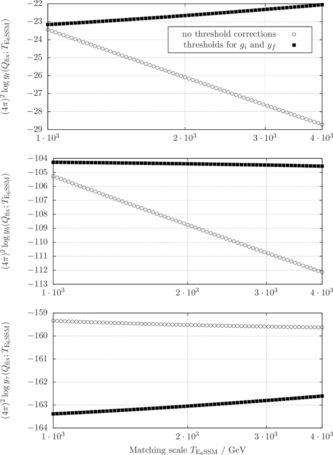
where Δg(Ti)Δ𝑔subscript𝑇𝑖\Delta g(T_{i}) can be obtained by matching Green functions of the full and the effective theory, see below. As a result the right-hand side of Eq. (12) will vanish, i.e. the gauge coupling gfull(Qfix)subscript𝑔fullsubscript𝑄fixg_{\text{full}}(Q_{\text{fix}}) will not depend on the matching scale. This property will be used as a test in Sec. 5.1.

To calculate the threshold corrections we consider a full theory consisting of parameters ρ1,,ρpsubscript𝜌1subscript𝜌𝑝\rho_{1},\dotsc,\rho_{p}, light fields l1,,lqsubscript𝑙1subscript𝑙𝑞l_{1},\dotsc,l_{q} and heavy fields H1,,Hrsubscript𝐻1subscript𝐻𝑟H_{1},\dotsc,H_{r}

full=full(ρ1,,ρp;l1,,lq,H1,,Hr).superscriptfullsuperscriptfullsubscript𝜌1subscript𝜌𝑝subscript𝑙1subscript𝑙𝑞subscript𝐻1subscript𝐻𝑟\displaystyle\mathcal{L}^{\text{full}}=\mathcal{L}^{\text{full}}(\rho_{1},\dotsc,\rho_{p};l_{1},\dotsc,l_{q},H_{1},\dotsc,H_{r}). (14)

The effective theory might contain effective parameters ρ^1,,ρ^ksubscript^𝜌1subscript^𝜌𝑘\hat{\rho}_{1},\dotsc,\hat{\rho}_{k} and effective light fields l^1,,l^qsubscript^𝑙1subscript^𝑙𝑞\hat{l}_{1},\dotsc,\hat{l}_{q}, where the heavy fields were integrated out

eff=eff(ρ^1,,ρ^k;l^1,,l^q).superscripteffsuperscripteffsubscript^𝜌1subscript^𝜌𝑘subscript^𝑙1subscript^𝑙𝑞\displaystyle\mathcal{L}^{\text{eff}}=\mathcal{L}^{\text{eff}}(\hat{\rho}_{1},\dotsc,\hat{\rho}_{k};\hat{l}_{1},\dotsc,\hat{l}_{q}). (15)

The requirement that both the full and the effective theory describe the same physics in the limit p0𝑝0p\rightarrow 0 can be achieved by equating all connected Green functions with light external fields lisubscript𝑙𝑖l_{i} in the full and in the effective theory at zero external momenta. This condition leads to the equality of all one-particle irreducible correlation functions ΓΓ\Gamma that are one-particle irreducible with respect to the light fields lisubscript𝑙𝑖l_{i} (1LPI)

Γli1li2linfull(ρ1,,ρp)|ki=0evaluated-atsubscriptsuperscriptΓfullsubscript𝑙subscript𝑖1subscript𝑙subscript𝑖2subscript𝑙subscript𝑖𝑛subscript𝜌1subscript𝜌𝑝subscript𝑘𝑖0\displaystyle\left.\Gamma^{\text{full}}_{l_{i_{1}}l_{i_{2}}\dotsm l_{i_{n}}}(\rho_{1},\dotsc,\rho_{p})\right|_{k_{i}=0} =Γli1li2lineff(ρ^1,,ρ^k)|ki=0,absentevaluated-atsubscriptsuperscriptΓeffsubscript𝑙subscript𝑖1subscript𝑙subscript𝑖2subscript𝑙subscript𝑖𝑛subscript^𝜌1subscript^𝜌𝑘subscript𝑘𝑖0\displaystyle=\left.\Gamma^{\text{eff}}_{l_{i_{1}}l_{i_{2}}\dotsm l_{i_{n}}}(\hat{\rho}_{1},\dotsc,\hat{\rho}_{k})\right|_{k_{i}=0}, (16)

where kisubscript𝑘𝑖k_{i} are the momenta of the external fields. The next step is to decompose the renormalized 1LPI correlation functions into a tree-level part and a part which contains one-loop contributions

Γli1li2linfullsubscriptsuperscriptΓfullsubscript𝑙subscript𝑖1subscript𝑙subscript𝑖2subscript𝑙subscript𝑖𝑛\displaystyle\Gamma^{\text{full}}_{l_{i_{1}}l_{i_{2}}\dotsm l_{i_{n}}} =Γli1li2linfull,tree+Γli1li2linfull,1L,absentsubscriptsuperscriptΓfull,treesubscript𝑙subscript𝑖1subscript𝑙subscript𝑖2subscript𝑙subscript𝑖𝑛subscriptsuperscriptΓfull,1Lsubscript𝑙subscript𝑖1subscript𝑙subscript𝑖2subscript𝑙subscript𝑖𝑛\displaystyle=\Gamma^{\text{\text{full},tree}}_{l_{i_{1}}l_{i_{2}}\dotsm l_{i_{n}}}+\Gamma^{\text{\text{full},1L}}_{l_{i_{1}}l_{i_{2}}\dotsm l_{i_{n}}}, (17)
Γli1li2lineffsubscriptsuperscriptΓeffsubscript𝑙subscript𝑖1subscript𝑙subscript𝑖2subscript𝑙subscript𝑖𝑛\displaystyle\Gamma^{\text{eff}}_{l_{i_{1}}l_{i_{2}}\dotsm l_{i_{n}}} =Γli1li2lineff,tree+Γli1li2lineff,1L.absentsubscriptsuperscriptΓeff,treesubscript𝑙subscript𝑖1subscript𝑙subscript𝑖2subscript𝑙subscript𝑖𝑛subscriptsuperscriptΓeff,1Lsubscript𝑙subscript𝑖1subscript𝑙subscript𝑖2subscript𝑙subscript𝑖𝑛\displaystyle=\Gamma^{\text{eff,tree}}_{l_{i_{1}}l_{i_{2}}\dotsm l_{i_{n}}}+\Gamma^{\text{eff,1L}}_{l_{i_{1}}l_{i_{2}}\dotsm l_{i_{n}}}. (18)

Imposing a relative field renormalization for the renormalized fields in the full and effective theory

l^isubscript^𝑙𝑖\displaystyle\hat{l}_{i} =(1+12Kli)li,(i=1,,q)absent112subscript𝐾subscript𝑙𝑖subscript𝑙𝑖𝑖1𝑞\displaystyle=\left(1+\frac{1}{2}K_{l_{i}}\right)l_{i},\qquad\qquad(i=1,\dotsc,q) (19)

and inserting Eq. (17)–(19) into (16) yields the matching condition

Γli1li2linfull,tree+Γli1li2linfull,1L=(1+12n=1qKlin)Γl^i1l^i2l^ineff,tree+Γl^i1l^i2l^ineff,1L+O(2).subscriptsuperscriptΓfull,treesubscript𝑙subscript𝑖1subscript𝑙subscript𝑖2subscript𝑙subscript𝑖𝑛subscriptsuperscriptΓfull,1Lsubscript𝑙subscript𝑖1subscript𝑙subscript𝑖2subscript𝑙subscript𝑖𝑛112superscriptsubscript𝑛1𝑞subscript𝐾subscript𝑙subscript𝑖𝑛subscriptsuperscriptΓeff,treesubscript^𝑙subscript𝑖1subscript^𝑙subscript𝑖2subscript^𝑙subscript𝑖𝑛subscriptsuperscriptΓeff,1Lsubscript^𝑙subscript𝑖1subscript^𝑙subscript𝑖2subscript^𝑙subscript𝑖𝑛𝑂superscriptPlanck-constant-over-2-pi2\displaystyle\Gamma^{\text{full,tree}}_{l_{i_{1}}l_{i_{2}}\dotsm l_{i_{n}}}+\Gamma^{\text{full,1L}}_{l_{i_{1}}l_{i_{2}}\dotsm l_{i_{n}}}=\left(1+\frac{1}{2}\sum_{n=1}^{q}K_{l_{i_{n}}}\right)\Gamma^{\text{eff,tree}}_{\hat{l}_{i_{1}}\hat{l}_{i_{2}}\dotsm\hat{l}_{i_{n}}}+\Gamma^{\text{eff,1L}}_{\hat{l}_{i_{1}}\hat{l}_{i_{2}}\dotsm\hat{l}_{i_{n}}}+O(\hbar^{2}). (20)

This equation is evaluated at zero external momenta. The analogous equation holds for the derivatives of the 1LPI correlation functions. Imposing all matching conditions yields the definitions for the Klisubscript𝐾subscript𝑙𝑖K_{l_{i}} in terms of 1LPI correlation functions and at the same time the desired relations between the parameters of the effective and full theory (threshold corrections)

ρ^i=ρi+Δρi(1-loop)(ρ1,,ρp,Kl1,,Klq),(i=1,,k).subscript^𝜌𝑖subscript𝜌𝑖Δsuperscriptsubscript𝜌𝑖(1-loop)subscript𝜌1subscript𝜌𝑝subscript𝐾subscript𝑙1subscript𝐾subscript𝑙𝑞𝑖1𝑘\displaystyle\hat{\rho}_{i}=\rho_{i}+\Delta\rho_{i}^{\text{(1-loop)}}(\rho_{1},\dotsc,\rho_{p},K_{l_{1}},\dotsc,K_{l_{q}}),\qquad\qquad(i=1,\dotsc,k). (21)

3.2 Gauge coupling threshold corrections in the E6SSM

Strong gauge coupling

To calculate the threshold correction for the gauge coupling g3subscript𝑔3g_{3} of the unbroken SU(3)c𝑆𝑈subscript3cSU(3)_{\text{c}} one needs to apply the matching procedure of Sec. 3.1 to the following 1LPI correlation functions

pΓqibarqiE6SSM(p,p)|p=0evaluated-atsubscript𝑝subscriptsuperscriptΓE6SSMsubscript𝑞𝑖barsubscript𝑞𝑖𝑝𝑝𝑝0\displaystyle\partial_{p}\left.\Gamma^{\text{E${}_{6}$SSM}}_{q_{i}\mathrm{bar}{q}_{i}}(p,-p)\right|_{p=0} =pΓqibarqiSM(p,p)|p=0,absentevaluated-atsubscript𝑝subscriptsuperscriptΓSMsubscript𝑞𝑖barsubscript𝑞𝑖𝑝𝑝𝑝0\displaystyle=\partial_{p}\left.\Gamma^{\text{SM}}_{q_{i}\mathrm{bar}{q}_{i}}(p,-p)\right|_{p=0}, (22)
k2ΓGμaGνbE6SSM(k,k)|k2=0evaluated-atsubscriptsuperscript𝑘2subscriptsuperscriptΓE6SSMsubscriptsuperscript𝐺𝑎𝜇subscriptsuperscript𝐺𝑏𝜈𝑘𝑘superscript𝑘20\displaystyle\partial_{k^{2}}\left.\Gamma^{\text{E${}_{6}$SSM}}_{G^{a}_{\mu}G^{b}_{\nu}}(k,-k)\right|_{k^{2}=0} =k2ΓGμaGνbSM(k,k)|k2=0,absentevaluated-atsubscriptsuperscript𝑘2subscriptsuperscriptΓSMsubscriptsuperscript𝐺𝑎𝜇subscriptsuperscript𝐺𝑏𝜈𝑘𝑘superscript𝑘20\displaystyle=\partial_{k^{2}}\left.\Gamma^{\text{SM}}_{G^{a}_{\mu}G^{b}_{\nu}}(k,-k)\right|_{k^{2}=0}, (23)
ΓGμaqibarqiE6SSM(k,p,(p+k))|p=k=0evaluated-atsubscriptsuperscriptΓE6SSMsubscriptsuperscript𝐺𝑎𝜇subscript𝑞𝑖barsubscript𝑞𝑖𝑘𝑝𝑝𝑘𝑝𝑘0\displaystyle\left.\Gamma^{\text{E${}_{6}$SSM}}_{G^{a}_{\mu}q_{i}\mathrm{bar}{q}_{i}}(k,p,-(p+k))\right|_{p=k=0} =ΓGμaqibarqiSM(k,p,(p+k))|p=k=0,absentevaluated-atsubscriptsuperscriptΓSMsubscriptsuperscript𝐺𝑎𝜇subscript𝑞𝑖barsubscript𝑞𝑖𝑘𝑝𝑝𝑘𝑝𝑘0\displaystyle=\left.\Gamma^{\text{SM}}_{G^{a}_{\mu}q_{i}\mathrm{bar}{q}_{i}}(k,p,-(p+k))\right|_{p=k=0}, (24)

where qisubscript𝑞𝑖q_{i} are the light colored fields that remain in the SM, i.e. the SM quarks. After imposing the relative field renormalizations (19) and decomposing the 1LPI functions into a tree-level and a loop part one gets the threshold correction for g3subscript𝑔3g_{3}

g3MS¯,SMsuperscriptsubscript𝑔3¯MSSM\displaystyle g_{3}^{\overline{\text{MS}},\text{SM}} =g3MS¯,E6SSM+g33(4π)2(f43FfC(rf)logmfμ+s13FsC(rs)logmsμ).absentsuperscriptsubscript𝑔3¯MSE6SSMsuperscriptsubscript𝑔33superscript4𝜋2subscript𝑓43subscript𝐹𝑓𝐶subscript𝑟𝑓subscript𝑚𝑓𝜇subscript𝑠13subscript𝐹𝑠𝐶subscript𝑟𝑠subscript𝑚𝑠𝜇\displaystyle=g_{3}^{\overline{\text{MS}},\text{E${}_{6}$SSM}}+\frac{g_{3}^{3}}{(4\pi)^{2}}\left(\sum_{f}\frac{4}{3}F_{f}C(r_{f})\log\frac{m_{f}}{\mu}+\sum_{s}\frac{1}{3}F_{s}C(r_{s})\log\frac{m_{s}}{\mu}\right). (25)

The sums run over all heavy fermions f𝑓f and scalars s𝑠s that are integrated out. Eq. (25) is also in agreement with the general result in [39]. The constants C(r)𝐶𝑟C(r) are invariants of the representations r𝑟r of SU(3)c𝑆𝑈subscript3cSU(3)_{\text{c}} and are given by

C(N)𝐶𝑁\displaystyle C(N) =12absent12\displaystyle=\frac{1}{2} (fundamental representation N),(fundamental representation N)\displaystyle\text{(fundamental representation $N$)}, (26)
C(G)𝐶𝐺\displaystyle C(G) =3absent3\displaystyle=3 (adjoint representation G),(adjoint representation G)\displaystyle\text{(adjoint representation $G$)}, (27)

and Ffsubscript𝐹𝑓F_{f}, Fssubscript𝐹𝑠F_{s} account for the different number of field degrees of freedom

Ffsubscript𝐹𝑓\displaystyle F_{f} ={1if f is a Dirac fermion,1/2if f is a Majorana fermion,absentcases1if f is a Dirac fermion12if f is a Majorana fermion\displaystyle=\begin{cases}1&\text{if $f$ is a Dirac fermion},\\ 1/2&\text{if $f$ is a Majorana fermion},\end{cases} (28)
Fssubscript𝐹𝑠\displaystyle F_{s} ={1if s is a complex scalar,1/2if s is a real scalar.absentcases1if s is a complex scalar12if s is a real scalar\displaystyle=\begin{cases}1&\text{if $s$ is a complex scalar},\\ 1/2&\text{if $s$ is a real scalar}.\end{cases} (29)

When matching the E6SSM to the SM, only the gluino, the squarks and the exotics contribute in Eq. (25) and we have

C(rg~)𝐶subscript𝑟~𝑔\displaystyle C(r_{\tilde{g}}) =C(G)=3,absent𝐶𝐺3\displaystyle=C(G)=3, C(rq~ik)𝐶subscript𝑟subscript~𝑞𝑖𝑘\displaystyle C(r_{\tilde{q}_{ik}}) =C(rD~ik)=C(rDi)=C(N)=1/2,absent𝐶subscript𝑟subscript~𝐷𝑖𝑘𝐶subscript𝑟subscript𝐷𝑖𝐶𝑁12\displaystyle=C(r_{\tilde{D}_{ik}})=C(r_{D_{i}})=C(N)=1/2, (30)
Fg~subscript𝐹~𝑔\displaystyle F_{\tilde{g}} =1/2,absent12\displaystyle=1/2, Fq~iksubscript𝐹subscript~𝑞𝑖𝑘\displaystyle F_{\tilde{q}_{ik}} =FD~ik=FDi=1.absentsubscript𝐹subscript~𝐷𝑖𝑘subscript𝐹subscript𝐷𝑖1\displaystyle=F_{\tilde{D}_{ik}}=F_{D_{i}}=1. (31)

Then the threshold correction (25) reduces to

g3DR¯,E6SSM=g3MS¯,SM+g33(4π)2[122logmg~μ16q~{u~,d~}i=13k=12logmq~ikμ23i=13logmDiμ16i=13k=12logmD~ikμ],superscriptsubscript𝑔3¯DRE6SSMsuperscriptsubscript𝑔3¯MSSMsuperscriptsubscript𝑔33superscript4𝜋2delimited-[]122subscript𝑚~𝑔𝜇16subscript~𝑞~𝑢~𝑑superscriptsubscript𝑖13superscriptsubscript𝑘12subscript𝑚subscript~𝑞𝑖𝑘𝜇23superscriptsubscript𝑖13subscript𝑚subscript𝐷𝑖𝜇16superscriptsubscript𝑖13superscriptsubscript𝑘12subscript𝑚subscript~𝐷𝑖𝑘𝜇\displaystyle\begin{split}g_{3}^{\overline{\text{DR}},\text{E${}_{6}$SSM}}=g_{3}^{\overline{\text{MS}},\text{SM}}+\frac{g_{3}^{3}}{(4\pi)^{2}}\Bigg{[}&\frac{1}{2}-2\log\frac{m_{\tilde{g}}}{\mu}-\frac{1}{6}\sum_{\tilde{q}\in\{\tilde{u},\tilde{d}\}}\sum_{i=1}^{3}\sum_{k=1}^{2}\log\frac{m_{\tilde{q}_{ik}}}{\mu}\\ &-\frac{2}{3}\sum_{i=1}^{3}\log\frac{m_{D_{i}}}{\mu}-\frac{1}{6}\sum_{i=1}^{3}\sum_{k=1}^{2}\log\frac{m_{\tilde{D}_{ik}}}{\mu}\Bigg{]},\end{split} (32)

where we have added a finite counterterm which converts g3subscript𝑔3g_{3} from the MS¯¯MS\overline{\text{MS}} to the DR¯¯DR\overline{\text{DR}} scheme [40].

Electroweak gauge couplings

The calculation of threshold corrections for the couplings gYsubscript𝑔𝑌g_{Y} and g2subscript𝑔2g_{2} is more involved, because the gauge group SU(2)L×U(1)Y𝑆𝑈subscript2L𝑈subscript1𝑌SU(2)_{\text{L}}\times U(1)_{Y} is spontaneously broken to U(1)em𝑈subscript1emU(1)_{\text{em}}. From the relations

gYsubscript𝑔𝑌\displaystyle g_{Y} =ecW,absent𝑒subscript𝑐𝑊\displaystyle=\frac{e}{c_{W}}, g2subscript𝑔2\displaystyle g_{2} =esW,absent𝑒subscript𝑠𝑊\displaystyle=\frac{e}{s_{W}}, cWsubscript𝑐𝑊\displaystyle c_{W} =mWmZabsentsubscript𝑚𝑊subscript𝑚𝑍\displaystyle=\frac{m_{W}}{m_{Z}} (33)

one can see that the threshold corrections for gYsubscript𝑔𝑌g_{Y} and g2subscript𝑔2g_{2} are related to those of the W±superscript𝑊plus-or-minusW^{\pm} and Z𝑍Z boson masses as well as to the gauge coupling e𝑒e of the remaining U(1)em𝑈subscript1emU(1)_{\text{em}} gauge symmetry. Therefore the following matching conditions are imposed to obtain threshold corrections for e𝑒e, mZsubscript𝑚𝑍m_{Z} and mWsubscript𝑚𝑊m_{W}

k2nΓWμ+WνE6SSM(k,k)|k2=0evaluated-atsuperscriptsubscriptsuperscript𝑘2𝑛subscriptsuperscriptΓE6SSMsubscriptsuperscript𝑊𝜇subscriptsuperscript𝑊𝜈𝑘𝑘superscript𝑘20\displaystyle\partial_{k^{2}}^{n}\left.\Gamma^{\text{E${}_{6}$SSM}}_{W^{+}_{\mu}W^{-}_{\nu}}(k,-k)\right|_{k^{2}=0} =k2nΓWμ+WνSM(k,k)|k2=0(n=0,1),absentevaluated-atsuperscriptsubscriptsuperscript𝑘2𝑛subscriptsuperscriptΓSMsubscriptsuperscript𝑊𝜇subscriptsuperscript𝑊𝜈𝑘𝑘superscript𝑘20𝑛01\displaystyle=\partial_{k^{2}}^{n}\left.\Gamma^{\text{SM}}_{W^{+}_{\mu}W^{-}_{\nu}}(k,-k)\right|_{k^{2}=0}\qquad(n=0,1), (34)
k2nΓZμZνE6SSM(k,k)|k2=0evaluated-atsuperscriptsubscriptsuperscript𝑘2𝑛subscriptsuperscriptΓE6SSMsubscript𝑍𝜇subscript𝑍𝜈𝑘𝑘superscript𝑘20\displaystyle\partial_{k^{2}}^{n}\left.\Gamma^{\text{E${}_{6}$SSM}}_{Z_{\mu}Z_{\nu}}(k,-k)\right|_{k^{2}=0} =k2nΓZμZνSM(k,k)|k2=0(n=0,1),absentevaluated-atsuperscriptsubscriptsuperscript𝑘2𝑛subscriptsuperscriptΓSMsubscript𝑍𝜇subscript𝑍𝜈𝑘𝑘superscript𝑘20𝑛01\displaystyle=\partial_{k^{2}}^{n}\left.\Gamma^{\text{SM}}_{Z_{\mu}Z_{\nu}}(k,-k)\right|_{k^{2}=0}\quad\qquad(n=0,1), (35)
k2ΓAμAνE6SSM(k,k)|k2=0evaluated-atsubscriptsuperscript𝑘2subscriptsuperscriptΓE6SSMsubscript𝐴𝜇subscript𝐴𝜈𝑘𝑘superscript𝑘20\displaystyle\partial_{k^{2}}\left.\Gamma^{\text{E${}_{6}$SSM}}_{A_{\mu}A_{\nu}}(k,-k)\right|_{k^{2}=0} =k2ΓAμAνSM(k,k)|k2=0,absentevaluated-atsubscriptsuperscript𝑘2subscriptsuperscriptΓSMsubscript𝐴𝜇subscript𝐴𝜈𝑘𝑘superscript𝑘20\displaystyle=\partial_{k^{2}}\left.\Gamma^{\text{SM}}_{A_{\mu}A_{\nu}}(k,-k)\right|_{k^{2}=0}, (36)
ΓZμAνE6SSM(k,k)|k2=0evaluated-atsubscriptsuperscriptΓE6SSMsubscript𝑍𝜇subscript𝐴𝜈𝑘𝑘superscript𝑘20\displaystyle\left.\Gamma^{\text{E${}_{6}$SSM}}_{Z_{\mu}A_{\nu}}(k,-k)\right|_{k^{2}=0} =ΓZμAνSM(k,k)|k2=0,absentevaluated-atsubscriptsuperscriptΓSMsubscript𝑍𝜇subscript𝐴𝜈𝑘𝑘superscript𝑘20\displaystyle=\left.\Gamma^{\text{SM}}_{Z_{\mu}A_{\nu}}(k,-k)\right|_{k^{2}=0}, (37)
pΓψLibarψLjE6SSM(p,p)|p=0evaluated-atsubscript𝑝subscriptsuperscriptΓE6SSMsubscript𝜓𝐿𝑖barsubscript𝜓𝐿𝑗𝑝𝑝𝑝0\displaystyle\partial_{p}\left.\Gamma^{\text{E${}_{6}$SSM}}_{\psi_{Li}\mathrm{bar}{\psi}_{Lj}}(p,-p)\right|_{p=0} =pΓψLibarψLjSM(p,p)|p=0,absentevaluated-atsubscript𝑝subscriptsuperscriptΓSMsubscript𝜓𝐿𝑖barsubscript𝜓𝐿𝑗𝑝𝑝𝑝0\displaystyle=\partial_{p}\left.\Gamma^{\text{SM}}_{\psi_{Li}\mathrm{bar}{\psi}_{Lj}}(p,-p)\right|_{p=0}, (38)
pΓψRibarψRjE6SSM(p,p)|p=0evaluated-atsubscript𝑝subscriptsuperscriptΓE6SSMsubscript𝜓𝑅𝑖barsubscript𝜓𝑅𝑗𝑝𝑝𝑝0\displaystyle\partial_{p}\left.\Gamma^{\text{E${}_{6}$SSM}}_{\psi_{Ri}\mathrm{bar}{\psi}_{Rj}}(p,-p)\right|_{p=0} =pΓψRibarψRjSM(p,p)|p=0,absentevaluated-atsubscript𝑝subscriptsuperscriptΓSMsubscript𝜓𝑅𝑖barsubscript𝜓𝑅𝑗𝑝𝑝𝑝0\displaystyle=\partial_{p}\left.\Gamma^{\text{SM}}_{\psi_{Ri}\mathrm{bar}{\psi}_{Rj}}(p,-p)\right|_{p=0}, (39)
ΓAμψibarψjE6SSM(k,p,(p+k))|k=p=0evaluated-atsubscriptsuperscriptΓE6SSMsubscript𝐴𝜇subscript𝜓𝑖barsubscript𝜓𝑗𝑘𝑝𝑝𝑘𝑘𝑝0\displaystyle\left.\Gamma^{\text{E${}_{6}$SSM}}_{A_{\mu}\psi_{i}\mathrm{bar}{\psi}_{j}}(k,p,-(p+k))\right|_{k=p=0} =ΓAμψibarψjSM(k,p,(p+k))|k=p=0.absentevaluated-atsubscriptsuperscriptΓSMsubscript𝐴𝜇subscript𝜓𝑖barsubscript𝜓𝑗𝑘𝑝𝑝𝑘𝑘𝑝0\displaystyle=\left.\Gamma^{\text{SM}}_{A_{\mu}\psi_{i}\mathrm{bar}{\psi}_{j}}(k,p,-(p+k))\right|_{k=p=0}. (40)

The additional matching condition for ΓZμAνsubscriptΓsubscript𝑍𝜇subscript𝐴𝜈\Gamma_{Z_{\mu}A_{\nu}} is necessary, because the gauge fields Bμsubscript𝐵𝜇B_{\mu}, Wμsubscript𝑊𝜇\vec{W}_{\mu} mix to Aμsubscript𝐴𝜇A_{\mu}, Zμsubscript𝑍𝜇Z_{\mu} and Wμ±subscriptsuperscript𝑊plus-or-minus𝜇W^{\pm}_{\mu}. Introducing relative field renormalizations for Wμ±subscriptsuperscript𝑊plus-or-minus𝜇W^{\pm}_{\mu}, Zμsubscript𝑍𝜇Z_{\mu}, Aμsubscript𝐴𝜇A_{\mu}, ψiLsubscript𝜓𝑖𝐿\psi_{iL} and ψiRsubscript𝜓𝑖𝑅\psi_{iR} and inserting them into the matching conditions (34)–(40) leads to the threshold corrections for the W𝑊W and Z𝑍Z boson masses and the electromagnetic coupling555The Ward identity which reflects the U(1)em𝑈subscript1emU(1)_{\text{em}} gauge invariance in the Standard Model was used to simplify the result.

(mVSM)2superscriptsuperscriptsubscript𝑚𝑉SM2\displaystyle(m_{V}^{\text{SM}})^{2} =(mVE6SSM)2+ΓVμVν,TE6SSM,1L,heavy|k2=0mV2KVV,V{W,Z},formulae-sequenceabsentsuperscriptsuperscriptsubscript𝑚𝑉E6SSM2evaluated-atsubscriptsuperscriptΓE6SSM,1L,heavysubscript𝑉𝜇subscript𝑉𝜈𝑇superscript𝑘20superscriptsubscript𝑚𝑉2subscript𝐾𝑉𝑉𝑉𝑊𝑍\displaystyle=(m_{V}^{\text{E${}_{6}$SSM}})^{2}+\left.\Gamma^{\text{E\textsubscript{6}SSM,1L,heavy}}_{V_{\mu}V_{\nu},T}\right|_{k^{2}=0}-m_{V}^{2}K_{VV},\qquad V\in\{W,Z\}, (41)
(mVE6SSM)2+ΔmV2,absentsuperscriptsuperscriptsubscript𝑚𝑉E6SSM2Δsuperscriptsubscript𝑚𝑉2\displaystyle\equiv(m_{V}^{\text{E${}_{6}$SSM}})^{2}+\Delta m_{V}^{2}, (42)
eSMsuperscript𝑒SM\displaystyle e^{\text{SM}} =eE6SSM(112KAAsW2cWKZA)eE6SSM+Δe.absentsuperscript𝑒E6SSM112subscript𝐾𝐴𝐴subscript𝑠𝑊2subscript𝑐𝑊subscript𝐾𝑍𝐴superscript𝑒E6SSMΔ𝑒\displaystyle=e^{\text{E${}_{6}$SSM}}\left(1-\frac{1}{2}K_{AA}-\frac{s_{W}}{2c_{W}}K_{ZA}\right)\equiv e^{\text{E${}_{6}$SSM}}+\Delta e. (43)

The relative field renormalization constants in Eq. (41) and (43) are given by

KAAsubscript𝐾𝐴𝐴\displaystyle K_{AA} =k2ΓAμAν,TE6SSM,1L,heavy|k2=0,absentevaluated-atsuperscript𝑘2subscriptsuperscriptΓE6SSM,1L,heavysubscript𝐴𝜇subscript𝐴𝜈𝑇superscript𝑘20\displaystyle=-\frac{\partial}{\partial k^{2}}\left.\Gamma^{\text{E\textsubscript{6}SSM,1L,heavy}}_{A_{\mu}A_{\nu},T}\right|_{k^{2}=0}, KZAsubscript𝐾𝑍𝐴\displaystyle K_{ZA} =2mZ2ΓAμZν,TE6SSM,1L,heavy|k2=0,absentevaluated-at2subscriptsuperscript𝑚2𝑍subscriptsuperscriptΓE6SSM,1L,heavysubscript𝐴𝜇subscript𝑍𝜈𝑇superscript𝑘20\displaystyle=\frac{2}{m^{2}_{Z}}\left.\Gamma^{\text{E\textsubscript{6}SSM,1L,heavy}}_{A_{\mu}Z_{\nu},T}\right|_{k^{2}=0}, (44)
KWWsubscript𝐾𝑊𝑊\displaystyle K_{WW} =k2ΓWμ+Wν,TE6SSM,1L,heavy|k2=0,absentevaluated-atsuperscript𝑘2subscriptsuperscriptΓE6SSM,1L,heavysubscriptsuperscript𝑊𝜇subscriptsuperscript𝑊𝜈𝑇superscript𝑘20\displaystyle=-\frac{\partial}{\partial k^{2}}\left.\Gamma^{\text{E\textsubscript{6}SSM,1L,heavy}}_{W^{+}_{\mu}W^{-}_{\nu},T}\right|_{k^{2}=0}, KZZsubscript𝐾𝑍𝑍\displaystyle K_{ZZ} =k2ΓZμZν,TE6SSM,1L,heavy|k2=0absentevaluated-atsuperscript𝑘2subscriptsuperscriptΓE6SSM,1L,heavysubscript𝑍𝜇subscript𝑍𝜈𝑇superscript𝑘20\displaystyle=-\frac{\partial}{\partial k^{2}}\left.\Gamma^{\text{E\textsubscript{6}SSM,1L,heavy}}_{Z_{\mu}Z_{\nu},T}\right|_{k^{2}=0} (45)

and by ΓVμVν,TE6SSM,1L,heavysubscriptsuperscriptΓE6SSM,1L,heavysubscript𝑉𝜇subscriptsuperscript𝑉𝜈𝑇\Gamma^{\text{E\textsubscript{6}SSM,1L,heavy}}_{V_{\mu}V^{\prime}_{\nu},T} we denote the one-loop parts of the gauge boson 2-point functions that contain all particles that we integrate out, i.e. all non-SM particles. Using Eq. (41)–(43) one can write the threshold corrections for gYsubscript𝑔𝑌g_{Y} and g2subscript𝑔2g_{2} in the form

gYSMsuperscriptsubscript𝑔𝑌SM\displaystyle g_{Y}^{\text{SM}} =eSMcWSM=eSMmZSMmWSM=gYE6SSM(1+Δee+12ΔmZ2mZ212ΔmW2mW2),absentsuperscript𝑒SMsuperscriptsubscript𝑐𝑊SMsuperscript𝑒SMsuperscriptsubscript𝑚𝑍SMsuperscriptsubscript𝑚𝑊SMsuperscriptsubscript𝑔𝑌E6SSM1Δ𝑒𝑒12Δsuperscriptsubscript𝑚𝑍2superscriptsubscript𝑚𝑍212Δsuperscriptsubscript𝑚𝑊2superscriptsubscript𝑚𝑊2\displaystyle=\frac{e^{\text{SM}}}{c_{W}^{\text{SM}}}=\frac{e^{\text{SM}}\,m_{Z}^{\text{SM}}}{m_{W}^{\text{SM}}}=g_{Y}^{\text{E${}_{6}$SSM}}\left(1+\frac{\Delta e}{e}+\frac{1}{2}\frac{\Delta m_{Z}^{2}}{m_{Z}^{2}}-\frac{1}{2}\frac{\Delta m_{W}^{2}}{m_{W}^{2}}\right), (46)
g2SMsuperscriptsubscript𝑔2SM\displaystyle g_{2}^{\text{SM}} =eSMsWSM=eSM1(mWSMmZSM)2=g2E6SSM(1+ΔeecW2sW2ΔmZ22mZ2+cW2sW2ΔmW22mW2).absentsuperscript𝑒SMsuperscriptsubscript𝑠𝑊SMsuperscript𝑒SM1superscriptsuperscriptsubscript𝑚𝑊SMsuperscriptsubscript𝑚𝑍SM2superscriptsubscript𝑔2E6SSM1Δ𝑒𝑒superscriptsubscript𝑐𝑊2superscriptsubscript𝑠𝑊2Δsuperscriptsubscript𝑚𝑍22superscriptsubscript𝑚𝑍2superscriptsubscript𝑐𝑊2superscriptsubscript𝑠𝑊2Δsuperscriptsubscript𝑚𝑊22superscriptsubscript𝑚𝑊2\displaystyle=\frac{e^{\text{SM}}}{s_{W}^{\text{SM}}}=\frac{e^{\text{SM}}}{\sqrt{1-\left(\frac{m_{W}^{\text{SM}}}{m_{Z}^{\text{SM}}}\right)^{2}}}=g_{2}^{\text{E${}_{6}$SSM}}\left(1+\frac{\Delta e}{e}-\frac{c_{W}^{2}}{s_{W}^{2}}\frac{\Delta m_{Z}^{2}}{2m_{Z}^{2}}+\frac{c_{W}^{2}}{s_{W}^{2}}\frac{\Delta m_{W}^{2}}{2m_{W}^{2}}\right). (47)

Inserting the explicit form of ΔeΔ𝑒\Delta e, ΔmW2Δsuperscriptsubscript𝑚𝑊2\Delta m_{W}^{2} and ΔmZ2Δsuperscriptsubscript𝑚𝑍2\Delta m_{Z}^{2} yields

gYDR¯,E6SSMsuperscriptsubscript𝑔𝑌¯DRE6SSM\displaystyle g_{Y}^{\overline{\text{DR}},\text{E${}_{6}$SSM}} =gYMS¯,SM+gY3(4π)2[43Nci=13(YDi2)2logmDiμ\displaystyle=g_{Y}^{\overline{\text{MS}},\text{SM}}+\frac{g_{Y}^{3}}{(4\pi)^{2}}\Bigg{[}-\frac{4}{3}N_{c}\sum_{i=1}^{3}\left(\frac{Y_{D_{i}}}{2}\right)^{2}\log\frac{m_{D_{i}}}{\mu}
13Nci=13k=12(YD~ik2)2logmD~ikμ13subscript𝑁𝑐superscriptsubscript𝑖13superscriptsubscript𝑘12superscriptsubscript𝑌subscript~𝐷𝑖𝑘22subscript𝑚subscript~𝐷𝑖𝑘𝜇\displaystyle\phantom{{}=}-\frac{1}{3}N_{c}\sum_{i=1}^{3}\sum_{k=1}^{2}\left(\frac{Y_{\tilde{D}_{ik}}}{2}\right)^{2}\log\frac{m_{\tilde{D}_{ik}}}{\mu}
13Nci=13k=L,R{(Yu~ik2)2logmu~ikμ+(Yd~ik2)2logmd~ikμ}13subscript𝑁𝑐superscriptsubscript𝑖13subscript𝑘𝐿𝑅superscriptsubscript𝑌subscript~𝑢𝑖𝑘22subscript𝑚subscript~𝑢𝑖𝑘𝜇superscriptsubscript𝑌subscript~𝑑𝑖𝑘22subscript𝑚subscript~𝑑𝑖𝑘𝜇\displaystyle\phantom{{}=}-\frac{1}{3}N_{c}\sum_{i=1}^{3}\sum_{k=L,R}\left\{\left(\frac{Y_{\tilde{u}_{ik}}}{2}\right)^{2}\log\frac{m_{\tilde{u}_{ik}}}{\mu}+\left(\frac{Y_{\tilde{d}_{ik}}}{2}\right)^{2}\log\frac{m_{\tilde{d}_{ik}}}{\mu}\right\}
13i=13k=L,R(Ye~ik2)2logme~ikμ13i=13(Yν~iL2)2logmν~iLμ13superscriptsubscript𝑖13subscript𝑘𝐿𝑅superscriptsubscript𝑌subscript~𝑒𝑖𝑘22subscript𝑚subscript~𝑒𝑖𝑘𝜇13superscriptsubscript𝑖13superscriptsubscript𝑌subscript~𝜈𝑖𝐿22subscript𝑚subscript~𝜈𝑖𝐿𝜇\displaystyle\phantom{{}=}-\frac{1}{3}\sum_{i=1}^{3}\sum_{k=L,R}\left(\frac{Y_{\tilde{e}_{ik}}}{2}\right)^{2}\log\frac{m_{\tilde{e}_{ik}}}{\mu}-\frac{1}{3}\sum_{i=1}^{3}\left(\frac{Y_{\tilde{\nu}_{iL}}}{2}\right)^{2}\log\frac{m_{\tilde{\nu}_{iL}}}{\mu}
13i=12p=12j=12(YHpij2)2logmHpijμ13j=12(YH23j2)2logmHμ13superscriptsubscript𝑖12superscriptsubscript𝑝12superscriptsubscript𝑗12superscriptsubscript𝑌superscriptsubscript𝐻𝑝𝑖𝑗22subscript𝑚superscriptsubscript𝐻𝑝𝑖𝑗𝜇13superscriptsubscript𝑗12superscriptsubscript𝑌superscriptsubscript𝐻23𝑗22subscript𝑚𝐻𝜇\displaystyle\phantom{{}=}-\frac{1}{3}\sum_{i=1}^{2}\sum_{p=1}^{2}\sum_{j=1}^{2}\left(\frac{Y_{H_{pi}^{j}}}{2}\right)^{2}\log\frac{m_{H_{pi}^{j}}}{\mu}-\frac{1}{3}\sum_{j=1}^{2}\left(\frac{Y_{H_{23}^{j}}}{2}\right)^{2}\log\frac{m_{H}}{\mu}
23i=13p=12j=12(YH~piLj2)2logmH~piLjμ23superscriptsubscript𝑖13superscriptsubscript𝑝12superscriptsubscript𝑗12superscriptsubscript𝑌superscriptsubscript~𝐻𝑝𝑖𝐿𝑗22subscript𝑚superscriptsubscript~𝐻𝑝𝑖𝐿𝑗𝜇\displaystyle\phantom{{}=}-\frac{2}{3}\sum_{i=1}^{3}\sum_{p=1}^{2}\sum_{j=1}^{2}\left(\frac{Y_{\tilde{H}_{piL}^{j}}}{2}\right)^{2}\log\frac{m_{\tilde{H}_{piL}^{j}}}{\mu}
13j=12(YHj2)2logmHjμ23j=12(YH~Lj2)2logmH~Ljμ13superscriptsubscript𝑗12superscriptsubscript𝑌superscriptsuperscript𝐻𝑗22subscript𝑚superscriptsuperscript𝐻𝑗𝜇23superscriptsubscript𝑗12superscriptsubscript𝑌superscriptsubscript~superscript𝐻𝐿𝑗22subscript𝑚superscriptsubscript~superscript𝐻𝐿𝑗𝜇\displaystyle\phantom{{}=}-\frac{1}{3}\sum_{j=1}^{2}\left(\frac{Y_{{H^{\prime}}^{j}}}{2}\right)^{2}\log\frac{m_{{H^{\prime}}^{j}}}{\mu}-\frac{2}{3}\sum_{j=1}^{2}\left(\frac{Y_{\tilde{H^{\prime}}_{L}^{j}}}{2}\right)^{2}\log\frac{m_{\tilde{H^{\prime}}_{L}^{j}}}{\mu}
13j=12(YbarHj2)2logmbarHjμ23j=12(YbarH~Lj2)2logmbarH~Ljμ],\displaystyle\phantom{{}=}-\frac{1}{3}\sum_{j=1}^{2}\left(\frac{Y_{\mathrm{bar}{H^{\prime}}^{j}}}{2}\right)^{2}\log\frac{m_{\mathrm{bar}{H^{\prime}}^{j}}}{\mu}-\frac{2}{3}\sum_{j=1}^{2}\left(\frac{Y_{{\tilde{\mathrm{bar}{H^{\prime}}}}_{L}^{j}}}{2}\right)^{2}\log\frac{m_{{\tilde{\mathrm{bar}{H^{\prime}}}}_{L}^{j}}}{\mu}\Bigg{]}, (48)
g2DR¯,E6SSM=g2MS¯,SM+g23(4π)2[\displaystyle g_{2}^{\overline{\text{DR}},\text{E${}_{6}$SSM}}=g_{2}^{\overline{\text{MS}},\text{SM}}+\frac{g_{2}^{3}}{(4\pi)^{2}}\Bigg{[} 1316Nci=13logmq~iLμ16i=13logm~iLμ1316subscript𝑁𝑐superscriptsubscript𝑖13subscript𝑚subscript~𝑞𝑖𝐿𝜇16superscriptsubscript𝑖13subscript𝑚subscript~𝑖𝐿𝜇\displaystyle\frac{1}{3}-\frac{1}{6}N_{c}\sum_{i=1}^{3}\log\frac{m_{\tilde{q}_{iL}}}{\mu}-\frac{1}{6}\sum_{i=1}^{3}\log\frac{m_{\tilde{\ell}_{iL}}}{\mu}
43logmW~μ16logmHμ43subscript𝑚~𝑊𝜇16subscript𝑚𝐻𝜇\displaystyle-\frac{4}{3}\log\frac{m_{\tilde{W}}}{\mu}-\frac{1}{6}\log\frac{m_{H}}{\mu}
16i=12p=12logmHpiμ13i=13p=12logmH~piLμ16superscriptsubscript𝑖12superscriptsubscript𝑝12subscript𝑚subscript𝐻𝑝𝑖𝜇13superscriptsubscript𝑖13superscriptsubscript𝑝12subscript𝑚subscript~𝐻𝑝𝑖𝐿𝜇\displaystyle-\frac{1}{6}\sum_{i=1}^{2}\sum_{p=1}^{2}\log\frac{m_{H_{pi}}}{\mu}-\frac{1}{3}\sum_{i=1}^{3}\sum_{p=1}^{2}\log\frac{m_{\tilde{H}_{piL}}}{\mu}
16logmHμ13logmH~Lμ16subscript𝑚superscript𝐻𝜇13subscript𝑚subscript~superscript𝐻𝐿𝜇\displaystyle-\frac{1}{6}\log\frac{m_{H^{\prime}}}{\mu}-\frac{1}{3}\log\frac{m_{\tilde{H^{\prime}}_{L}}}{\mu}
16logmbarHμ13logmbarH~Lμ],\displaystyle-\frac{1}{6}\log\frac{m_{\mathrm{bar}{H^{\prime}}}}{\mu}-\frac{1}{3}\log\frac{m_{\tilde{\mathrm{bar}{H^{\prime}}}_{L}}}{\mu}\Bigg{]}, (49)

where we have added a finite counterterm which converts g2subscript𝑔2g_{2} from the MS¯¯MS\overline{\text{MS}} to the DR¯¯DR\overline{\text{DR}} scheme [40] and neglected mixing.

3.3 Yukawa couplings in the E6SSM

Since the SM fermion masses are measured but not the Yukawa couplings, we don’t define the E6SSM Yukawa couplings in terms of threshold corrections to the running SM Yukawa couplings. Instead we directly match them at the one-loop level to the measured SM fermion masses and gauge couplings via

ytDR¯,E6SSMsuperscriptsubscript𝑦𝑡¯DRE6SSM\displaystyle y_{t}^{\overline{\text{DR}},\text{E${}_{6}$SSM}} =g2DR¯,E6SSMmton-shell,SM2mWon-shell,SMsinβ(1δmWmWon-shell,SM+δmtmton-shell,SM),absentsuperscriptsubscript𝑔2¯DRE6SSMsuperscriptsubscript𝑚𝑡on-shell,SM2superscriptsubscript𝑚𝑊on-shell,SM𝛽1𝛿subscript𝑚𝑊superscriptsubscript𝑚𝑊on-shell,SM𝛿subscript𝑚𝑡superscriptsubscript𝑚𝑡on-shell,SM\displaystyle=\frac{g_{2}^{\overline{\text{DR}},\text{E${}_{6}$SSM}}m_{t}^{\text{on-shell,SM}}}{\sqrt{2}m_{W}^{\text{on-shell,SM}}\sin{\beta}}\left(1-\frac{\delta m_{W}}{m_{W}^{\text{on-shell,SM}}}+\frac{\delta m_{t}}{m_{t}^{\text{on-shell,SM}}}\right), (50)
ybDR¯,E6SSMsuperscriptsubscript𝑦𝑏¯DRE6SSM\displaystyle y_{b}^{\overline{\text{DR}},\text{E${}_{6}$SSM}} =g2DR¯,E6SSMmbDR¯,(5)(mZ)2mWon-shell,SMcosβ(1δmWmWon-shell,SM+δmbδmb(5)+δmbshiftmbDR¯,(5)(mZ)),absentsuperscriptsubscript𝑔2¯DRE6SSMsuperscriptsubscript𝑚𝑏DR¯,(5)subscript𝑚𝑍2superscriptsubscript𝑚𝑊on-shell,SM𝛽1𝛿subscript𝑚𝑊superscriptsubscript𝑚𝑊on-shell,SM𝛿subscript𝑚𝑏𝛿superscriptsubscript𝑚𝑏5𝛿superscriptsubscript𝑚𝑏shiftsuperscriptsubscript𝑚𝑏DR¯,(5)subscript𝑚𝑍\displaystyle=\frac{g_{2}^{\overline{\text{DR}},\text{E${}_{6}$SSM}}m_{b}^{\text{$\overline{\text{DR}}$,(5)}}(m_{Z})}{\sqrt{2}m_{W}^{\text{on-shell,SM}}\cos{\beta}}\left(1-\frac{\delta m_{W}}{m_{W}^{\text{on-shell,SM}}}+\frac{\delta m_{b}-\delta m_{b}^{(5)}+\delta m_{b}^{\text{shift}}}{m_{b}^{\text{$\overline{\text{DR}}$,(5)}}(m_{Z})}\right), (51)
yτDR¯,E6SSMsuperscriptsubscript𝑦𝜏¯DRE6SSM\displaystyle y_{\tau}^{\overline{\text{DR}},\text{E${}_{6}$SSM}} =g2DR¯,E6SSMmτon-shell,SM2mWon-shell,SMcosβ(1δmWmWon-shell,SM+δmτmτon-shell,SM).absentsuperscriptsubscript𝑔2¯DRE6SSMsuperscriptsubscript𝑚𝜏on-shell,SM2superscriptsubscript𝑚𝑊on-shell,SM𝛽1𝛿subscript𝑚𝑊superscriptsubscript𝑚𝑊on-shell,SM𝛿subscript𝑚𝜏superscriptsubscript𝑚𝜏on-shell,SM\displaystyle=\frac{g_{2}^{\overline{\text{DR}},\text{E${}_{6}$SSM}}m_{\tau}^{\text{on-shell,SM}}}{\sqrt{2}m_{W}^{\text{on-shell,SM}}\cos{\beta}}\left(1-\frac{\delta m_{W}}{m_{W}^{\text{on-shell,SM}}}+\frac{\delta m_{\tau}}{m_{\tau}^{\text{on-shell,SM}}}\right). (52)

Here mton-shell,SMsuperscriptsubscript𝑚𝑡on-shell,SMm_{t}^{\text{on-shell,SM}}, mτon-shell,SMsuperscriptsubscript𝑚𝜏on-shell,SMm_{\tau}^{\text{on-shell,SM}} and mWon-shell,SMsuperscriptsubscript𝑚𝑊on-shell,SMm_{W}^{\text{on-shell,SM}} are Standard Model on-shell masses [41]. To avoid large logarithms from the bottom mass we use the DR¯¯DR\overline{\text{DR}} value of mbsubscript𝑚𝑏m_{b} in the 5-flavor QCD at mZsubscript𝑚𝑍m_{Z}, mbDR¯,(5)(mZ)=2.83 GeVsuperscriptsubscript𝑚𝑏DR¯,(5)subscript𝑚𝑍times2.83gigaelectronvoltm_{b}^{\text{$\overline{\text{DR}}$,(5)}}(m_{Z})=$2.83\text{\,}\mathrm{GeV}$ [42] which we then shift to the scale μ𝜇\mu where the Yukawa couplings are evaluated at. The counterterms in Eqs. (50)–(52) are defined as

δmf𝛿subscript𝑚𝑓\displaystyle\delta m_{f} =δmfon-shell,E6SSMδmfDR¯,E6SSMabsent𝛿superscriptsubscript𝑚𝑓on-shellE6SSM𝛿superscriptsubscript𝑚𝑓¯DRE6SSM\displaystyle=\delta m_{f}^{\text{on-shell},\text{E${}_{6}$SSM}}-\delta m_{f}^{\overline{\text{DR}},\text{E${}_{6}$SSM}} =e~Σf(mf2)|finite(f=t,b,τ),absentevaluated-at~esubscriptΣ𝑓superscriptsubscript𝑚𝑓2finite𝑓𝑡𝑏𝜏\displaystyle=\left.\operatorname{\widetilde{\Re e}}\Sigma_{f}(m_{f}^{2})\right|_{\text{finite}}\qquad(f=t,b,\tau), (53)
δmb(5)𝛿superscriptsubscript𝑚𝑏5\displaystyle\delta m_{b}^{(5)} =δmbon-shell,QCD(5)δmbDR¯,(5)absent𝛿superscriptsubscript𝑚𝑏on-shell,QCD(5)𝛿superscriptsubscript𝑚𝑏¯DR5\displaystyle=\delta m_{b}^{\text{on-shell,QCD(5)}}-\delta m_{b}^{\overline{\text{DR}},(5)} =4mbDR¯,(5)(mZ)3(4π)2g32(5+3logμ2mb2),absent4superscriptsubscript𝑚𝑏DR¯,(5)subscript𝑚𝑍3superscript4𝜋2superscriptsubscript𝑔3253superscript𝜇2superscriptsubscript𝑚𝑏2\displaystyle=-\frac{4m_{b}^{\text{$\overline{\text{DR}}$,(5)}}(m_{Z})}{3(4\pi)^{2}}g_{3}^{2}\left(5+3\log\frac{\mu^{2}}{m_{b}^{2}}\right), (54)
δmbshift𝛿superscriptsubscript𝑚𝑏shift\displaystyle\delta m_{b}^{\text{shift}} =βmbDR¯,(5)logμmZabsentsuperscriptsubscript𝛽subscript𝑚𝑏¯DR5𝜇subscript𝑚𝑍\displaystyle=\beta_{m_{b}}^{\overline{\text{DR}},(5)}\log\frac{\mu}{m_{Z}} =2mbDR¯,(5)(mZ)g324π2logμmZ,absent2superscriptsubscript𝑚𝑏DR¯,(5)subscript𝑚𝑍superscriptsubscript𝑔324superscript𝜋2𝜇subscript𝑚𝑍\displaystyle=-2m_{b}^{\text{$\overline{\text{DR}}$,(5)}}(m_{Z})\frac{g_{3}^{2}}{4\pi^{2}}\log\frac{\mu}{m_{Z}}, (55)
δmW𝛿subscript𝑚𝑊\displaystyle\delta m_{W} =δmWon-shell,E6SSMδmWDR¯,E6SSMabsent𝛿superscriptsubscript𝑚𝑊on-shellE6SSM𝛿superscriptsubscript𝑚𝑊¯DRE6SSM\displaystyle=\delta m_{W}^{\text{on-shell},\text{E${}_{6}$SSM}}-\delta m_{W}^{\overline{\text{DR}},\text{E${}_{6}$SSM}} =e~ΠWW,T(mW2)|finite.absentevaluated-at~esubscriptΠ𝑊𝑊𝑇superscriptsubscript𝑚𝑊2finite\displaystyle=\left.\operatorname{\widetilde{\Re e}}\Pi_{WW,T}(m_{W}^{2})\right|_{\text{finite}}. (56)

The self-energies ΣfsubscriptΣ𝑓\Sigma_{f} and ΠWW,TsubscriptΠ𝑊𝑊𝑇\Pi_{WW,T} are listed in Appendix C. It was checked that the divergences of (50)–(52), see Appendix D, are in agreement with the prediction from the one-loop RGEs.

4 Obtaining accurate spectra in the CE6SSM

4.1 The CE6SSM and its parameters

The threshold corrections presented in the previous section improve the precision of the high-scale–low-scale connection in the general E6SSM. In the present paper we apply them to the constrained version of the E6SSM (CE6SSM). The CE6SSM is defined by a universal scalar mass m0subscript𝑚0m_{0}, gaugino mass M1/2subscript𝑀12M_{1/2} and trilinear mass A𝐴A at the gauge coupling unification scale MXsubscript𝑀𝑋M_{X} [8, 9]. Owing to the unification of matter and Higgs fields in complete GUT multiplets these constraints are particularly well motivated. The soft scalar masses from the survival Higgs (which appear in the incomplete (𝟐𝟕)superscript27(\mathbf{27})^{\prime} and (𝟐𝟕¯)superscript¯27(\mathbf{\overline{27}})^{\prime} representations) sector, mHsubscript𝑚superscript𝐻m_{H^{\prime}}, mbarHsubscript𝑚barsuperscript𝐻m_{\mathrm{bar}{H^{\prime}}} are not assumed to be unified with m0subscript𝑚0m_{0} and the soft bilinear Bμ𝐵superscript𝜇B\mu^{\prime} is also unconstrained.

The CE6SSM is an example of a highly predictive, non-minimal SUSY model. It contains many new states at the TeV scale but has only few free parameters. In theory, the CE6SSM is fully determined by specifying the gauge couplings, the superpotential parameters yt,b,τsubscript𝑦𝑡𝑏𝜏y_{t,b,\tau}, λisubscript𝜆𝑖\lambda_{i} and κisubscript𝜅𝑖\kappa_{i} and the universal soft parameters m0subscript𝑚0m_{0}, M1/2subscript𝑀12M_{1/2}, A𝐴A at the GUT scale as well as the survival Higgs parameters. All high-scale parameters are shown in the top row of boxes in Fig. 2.

In practice, the model predictions of course need to agree with known SM constraints, in particular with the four known masses mZsubscript𝑚𝑍m_{Z}, mt,b,τsubscript𝑚𝑡𝑏𝜏m_{t,b,\tau} and the known low-energy gauge couplings. Furthermore, it is useful to take the low-energy values of tanβ=vu/vd𝛽subscript𝑣𝑢subscript𝑣𝑑\tan\beta=v_{u}/v_{d} and s=2S𝑠2delimited-⟨⟩𝑆s=\sqrt{2}\langle S\rangle as free parameters of the model. In this way, the six GUT-scale parameters m0subscript𝑚0m_{0}, M1/2subscript𝑀12M_{1/2}, A𝐴A and yt,b,τsubscript𝑦𝑡𝑏𝜏y_{t,b,\tau} are traded for the four known SM mass constraints and the two low-scale input parameters tanβ𝛽\tan\beta and s𝑠s. Compared to the familiar CMSSM, the CE6SSM has no μ𝜇\mu and Bμ𝐵𝜇B\mu parameters, which could be adjusted to fulfill SM constraints. Hence, the CMSSM input parameters m0subscript𝑚0m_{0}, M1/2subscript𝑀12M_{1/2} and A𝐴A are calculable in the CE6SSM.

Fig. 2 shows the resulting structure of input and output of the CE6SSM and the connection of the high and low scales. High-scale input parameters are the superpotential parameters λi(MX)subscript𝜆𝑖subscript𝑀𝑋\lambda_{i}(M_{X}) and κi(MX)subscript𝜅𝑖subscript𝑀𝑋\kappa_{i}(M_{X}); low-scale input parameters are s(Qfix)𝑠subscript𝑄fixs(Q_{\text{fix}}), tanβ(Qfix)𝛽subscript𝑄fix\tan\beta(Q_{\text{fix}}) and the survival Higgs parameters (defined at the matching scale TE6SSMsubscript𝑇E6SSMT_{\text{E${}_{6}$SSM}}), all defined in the DR¯¯DR\overline{\text{DR}} scheme. The low-scale SM constraints fix the remaining parameters. In previous studies λisubscript𝜆𝑖\lambda_{i}, κisubscript𝜅𝑖\kappa_{i}, s𝑠s and tanβ𝛽\tan\beta were sufficient to fix the spectrum. Here, with the inclusion of threshold corrections, we will be able to study the perturbation caused by the survival Higgs sector as well.

As the Figure shows, 6+3+4=13634136+3+4=13 high-scale parameters have been traded against these 131313 low-scale input parameters, so this high- and low-scale input determines the structure of the model completely and at all scales. The fixed scale Qfixsubscript𝑄fixQ_{\text{fix}}, where s𝑠s and tanβ𝛽\tan\beta are defined at, is set in Sec. 5 to a value of the order of the matching scale TE6SSMsubscript𝑇E6SSMT_{\text{E${}_{6}$SSM}}.

Refer to caption
Fig. 2: The structure of high- and low-scale input and output of the CE6SSM.

4.2 Numerical procedure and the improved spectrum generator

We extended the particle spectrum generator previously written for [8], which is partly based on SOFTSUSY 2.0.5 [24]. As input the program gets a CE6SSM parameter point specified by the high- and low-scale input

λ1,2,3(MX),κ1,2,3(MX),s(Qfix),tanβ(Qfix),μ(TE6SSM),mH(TE6SSM),mbarH(TE6SSM),Bμ(TE6SSM),subscript𝜆123subscript𝑀𝑋subscript𝜅123subscript𝑀𝑋𝑠subscript𝑄fix𝛽subscript𝑄fixsuperscript𝜇subscript𝑇E6SSMsubscript𝑚superscript𝐻subscript𝑇E6SSMsubscript𝑚barsuperscript𝐻subscript𝑇E6SSM𝐵superscript𝜇subscript𝑇E6SSM\displaystyle\begin{split}\lambda_{1,2,3}(M_{X}),\kappa_{1,2,3}(M_{X}),s(Q_{\text{fix}}),\tan\beta(Q_{\text{fix}}),\\ \mu^{\prime}(T_{\text{E${}_{6}$SSM}}),m_{H^{\prime}}(T_{\text{E${}_{6}$SSM}}),m_{\mathrm{bar}{H}^{\prime}}(T_{\text{E${}_{6}$SSM}}),B\mu^{\prime}(T_{\text{E${}_{6}$SSM}}),\end{split} (57)

and the program knows about the SM constraints discussed above. As illustrated in Fig. 2, RGEs and threshold corrections connect high and low scales, and the aim is to find output parameters consistent with the given input and then to compute the physical particle masses from the obtained low-energy SUSY breaking parameters. However, the threshold corrections can only be computed once the full mass spectrum is known. Hence, these steps need to be iterated until convergence is reached, and in the first iteration the threshold corrections must be ignored.

In the actual computation, we divide the basic strategy of each iteration into five steps, see Fig. 3. The details are as follows.

Refer to caption
Fig. 3: Program flow chart. The dashed box marks the structure of the old spectrum generator, which had no threshold corrections.
  1. 1.

    Determine the gauge and Yukawa couplings in the E6SSM at the threshold scale TE6SSMsubscript𝑇E6SSMT_{\text{E${}_{6}$SSM}} from the known SM gauge couplings and masses, using SM RGEs and the threshold corrections.

    1. (a)

      Evolve the SM MS¯¯MS\overline{\text{MS}} gauge and Yukawa couplings from their known values at mZsubscript𝑚𝑍m_{Z} [41] to the intermediate matching scale TE6SSMsubscript𝑇E6SSMT_{\text{E${}_{6}$SSM}} using SM RGEs.

    2. (b)

      Convert the SM MS¯¯MS\overline{\text{MS}} couplings to E6SSM DR¯¯DR\overline{\text{DR}} couplings using the individual particle threshold corrections discussed in Sec. 3. This step is only possible once the physical particle masses are known, i.e. after the first iteration. Hence, in the first iteration, the threshold corrections are replaced by the trivial definitions

      yfE6SSMsuperscriptsubscript𝑦𝑓E6SSM\displaystyle y_{f}^{\text{E${}_{6}$SSM}} :=yfSMcosβ(f=b,τ),assignabsentsuperscriptsubscript𝑦𝑓SM𝛽𝑓𝑏𝜏\displaystyle:=\frac{y_{f}^{\text{SM}}}{\cos\beta}\ (f=b,\tau), ytE6SSMsuperscriptsubscript𝑦𝑡E6SSM\displaystyle y_{t}^{\text{E${}_{6}$SSM}} :=ytSMsinβ,assignabsentsuperscriptsubscript𝑦𝑡SM𝛽\displaystyle:=\frac{y_{t}^{\text{SM}}}{\sin\beta}, (58)
      giDR¯,E6SSMsuperscriptsubscript𝑔𝑖DR¯,E6SSM\displaystyle g_{i}^{\text{$\overline{\text{DR}}$,\text{E${}_{6}$SSM}}} :=giMS¯,SM(i=1,2,3).assignabsentsuperscriptsubscript𝑔𝑖MS¯,SM𝑖123\displaystyle:=g_{i}^{\text{$\overline{\text{MS}}$,\text{SM}}}\ (i=1,2,3). (59)

      Note that, in contrast to Ref. [8], we do not use an intermediate matching to the MSSM because the MSSM and the E6SSM spectra are typically mixed.

  2. 2.

    Use RGEs to determine the high-scale gauge and Yukawa couplings and the low-scale values of the λisubscript𝜆𝑖\lambda_{i}, κisubscript𝜅𝑖\kappa_{i}. This step is completely independent of all soft SUSY breaking parameters because of the structure of the RGEs.

    1. (a)

      Estimate low-energy values for the Yukawa couplings λi(TE6SSM)subscript𝜆𝑖subscript𝑇E6SSM\lambda_{i}(T_{\text{E${}_{6}$SSM}}), κi(TE6SSM)subscript𝜅𝑖subscript𝑇E6SSM\kappa_{i}(T_{\text{E${}_{6}$SSM}}). The necessity of this estimate is an additional complication not present e.g. in the CMSSM. The difference is due to the fact that in the CMSSM all high-scale input parameters are soft breaking parameters, while here they are superpotential parameters.

    2. (b)

      Evolve all E6SSM gauge and Yukawa couplings from TE6SSMsubscript𝑇E6SSMT_{\text{E${}_{6}$SSM}} up to the unification scale MXsubscript𝑀𝑋M_{X}, defined as the scale where g1=g2subscript𝑔1subscript𝑔2g_{1}=g_{2}, using two-loop E6SSM RGEs.

    3. (c)

      Set Yukawa couplings λi(MX)subscript𝜆𝑖subscript𝑀𝑋\lambda_{i}(M_{X}), κi(MX)subscript𝜅𝑖subscript𝑀𝑋\kappa_{i}(M_{X}) to program input values.

    4. (d)

      Set gN:=g0/40assignsubscript𝑔𝑁subscript𝑔040g_{N}:=g_{0}/\sqrt{40}, where g0subscript𝑔0g_{0} is defined by g1(MX)subscript𝑔1subscript𝑀𝑋g_{1}(M_{X}).

    5. (e)

      Perform an iteration between MXsubscript𝑀𝑋M_{X} and TE6SSMsubscript𝑇E6SSMT_{\text{E${}_{6}$SSM}} to obtain values for the gauge and Yukawa couplings and λisubscript𝜆𝑖\lambda_{i}, κisubscript𝜅𝑖\kappa_{i} until consistency is reached with low-energy boundary conditions yf(TE6SSM)subscript𝑦𝑓subscript𝑇E6SSMy_{f}(T_{\text{E${}_{6}$SSM}}), gi(TE6SSM)subscript𝑔𝑖subscript𝑇E6SSMg_{i}(T_{\text{E${}_{6}$SSM}}) and high energy boundary conditions λi(MX)subscript𝜆𝑖subscript𝑀𝑋\lambda_{i}(M_{X}), κi(MX)subscript𝜅𝑖subscript𝑀𝑋\kappa_{i}(M_{X}).

  3. 3.

    With the gauge, Yukawa and λisubscript𝜆𝑖\lambda_{i}, κisubscript𝜅𝑖\kappa_{i} couplings now known at all scales we find solutions for the soft breaking parameters. They are determined by the high-scale constraints of universal m0subscript𝑚0m_{0}, M1/2subscript𝑀12M_{1/2}, A𝐴A, and by low-scale electroweak symmetry breaking (EWSB) conditions, i.e. consistency with the measured value of mZsubscript𝑚𝑍m_{Z} and the input values for tanβ𝛽\tan\beta and s𝑠s. First, the dependency of the low-energy soft mass parameters on the GUT scale values m02subscriptsuperscript𝑚20m^{2}_{0}, M1/2subscript𝑀12M_{1/2}, A0subscript𝐴0A_{0} is expressed in terms of the semi-analytical formulas

    mi2(t)subscriptsuperscript𝑚2𝑖𝑡\displaystyle m^{2}_{i}(t) =ai(t)m02+bi(t)M1/22+ci(t)A0M1/2+di(t)A02,absentsubscript𝑎𝑖𝑡subscriptsuperscript𝑚20subscript𝑏𝑖𝑡subscriptsuperscript𝑀212subscript𝑐𝑖𝑡subscript𝐴0subscript𝑀12subscript𝑑𝑖𝑡subscriptsuperscript𝐴20\displaystyle=a_{i}(t)m^{2}_{0}+b_{i}(t)M^{2}_{1/2}+c_{i}(t)A_{0}M_{1/2}+d_{i}(t)A^{2}_{0}, (60)
    Ai(t)subscript𝐴𝑖𝑡\displaystyle A_{i}(t) =ei(t)A0+fi(t)M1/2,absentsubscript𝑒𝑖𝑡subscript𝐴0subscript𝑓𝑖𝑡subscript𝑀12\displaystyle=e_{i}(t)A_{0}+f_{i}(t)M_{1/2}, (61)
    Mi(t)subscript𝑀𝑖𝑡\displaystyle M_{i}(t) =pi(t)A0+qi(t)M1/2,absentsubscript𝑝𝑖𝑡subscript𝐴0subscript𝑞𝑖𝑡subscript𝑀12\displaystyle=p_{i}(t)A_{0}+q_{i}(t)M_{1/2}, (62)

    where the coefficients ai(t),,qi(t)subscript𝑎𝑖𝑡subscript𝑞𝑖𝑡a_{i}(t),\dotsc,q_{i}(t) are calculated numerically at the scale t=logTE6SSM/MX𝑡subscript𝑇E6SSMsubscript𝑀𝑋t=\log T_{\text{E${}_{6}$SSM}}/M_{X}.

  4. 4.

    Next, the EWSB conditions are used to fix the values of the soft parameters.

    1. (a)

      The obtained expressions for the low-energy soft parameters mi2(t)subscriptsuperscript𝑚2𝑖𝑡m^{2}_{i}(t), Mi(t)subscript𝑀𝑖𝑡M_{i}(t), Ai(t)subscript𝐴𝑖𝑡A_{i}(t) are then combined with tree level EWSB conditions

      Vv1=Vv2=Vs=0𝑉subscript𝑣1𝑉subscript𝑣2𝑉𝑠0\displaystyle\frac{\partial V}{\partial v_{1}}=\frac{\partial V}{\partial v_{2}}=\frac{\partial V}{\partial s}=0 (63)

      and the known values of mZsubscript𝑚𝑍m_{Z}, tanβ𝛽\tan\beta and s𝑠s to form three quadratic equations in the soft masses m0subscript𝑚0m_{0}, M1/2subscript𝑀12M_{1/2} and A𝐴A, which can be reduced to a single quartic equation.

    2. (b)

      This quartic equation is then solved numerically and the values used to determine the mass spectra. Note that in principle there will be four solutions, though some or all may be complex. Therefore our routine deals with between zero and four sets of real solutions.

    3. (c)

      Tadpole corrections can now be calculated and added to the EWSB conditions, and a solution of consistent EWSB for the leading one-loop effective potential is found iteratively.

  5. 5.

    The full CE6SSM particle mass spectrum is now determined for each set of {m02,M1/2,A0}subscriptsuperscript𝑚20subscript𝑀12subscript𝐴0\{m^{2}_{0},M_{1/2},A_{0}\} found to be consistent with both high scale and low scale boundary conditions.

The final solution is found by iterating over all five steps until convergent solutions are obtained.

It is important to note that in general EWSB is not guaranteed in the CE6SSM, i.e. solutions for {m02,M1/2,A0}subscriptsuperscript𝑚20subscript𝑀12subscript𝐴0\{m^{2}_{0},M_{1/2},A_{0}\} from Eq. (63) are not always found. But for sufficiently large values of κisubscript𝜅𝑖\kappa_{i} the soft parameter mS2subscriptsuperscript𝑚2𝑆m^{2}_{S} always gets negative at low energies, which triggers EWSB [8].

5 Results

In this section we present the results obtained with our improved CE6SSM spectrum generator. We start by quantifying how the threshold corrections stabilize the results for parameters like gauge couplings and the mass spectrum. We will then extensively discuss the resulting, more accurate mass spectrum. On the one hand we will obtain more precise information on previously defined benchmark points, implying that some are now excluded by LHC data. On the other hand we scan over the parameter space and find large regions which are compatible with LHC limits on SUSY particles and are consistent with the latest discovery of the new boson which we associate with the lightest Higgs boson in the model. Finally we investigate the impact of the survival Higgs sector, which is possible due to the threshold corrections. It has implications on gauge coupling unification and on the predictions for the low-energy mass spectrum. In subsequent studies we sometimes make use of a test point, PP1, to illustrate effects, which is defined by,

tanβ(Qfix)=35,λ1,2,3(MX)=κ1,2,3(MX)=0.2,s(Qfix)=10 TeV,μ(TE6SSM)=mH(TE6SSM)=mbarH(TE6SSM)=10 TeV,Bμ(TE6SSM)=0.formulae-sequenceformulae-sequence𝛽subscript𝑄fix35subscript𝜆123subscript𝑀𝑋subscript𝜅123subscript𝑀𝑋0.2formulae-sequence𝑠subscript𝑄fixtimes10teraelectronvoltsuperscript𝜇subscript𝑇E6SSMsubscript𝑚superscript𝐻subscript𝑇E6SSMsubscript𝑚barsuperscript𝐻subscript𝑇E6SSMtimes10teraelectronvolt𝐵superscript𝜇subscript𝑇E6SSM0\displaystyle\begin{split}\tan\beta(Q_{\text{fix}})=35,\lambda_{1,2,3}(M_{X})=\kappa_{1,2,3}(M_{X})=0.2,s(Q_{\text{fix}})=$10\text{\,}\mathrm{TeV}$,\\ \mu^{\prime}(T_{\text{E${}_{6}$SSM}})=m_{H^{\prime}}(T_{\text{E${}_{6}$SSM}})=m_{\mathrm{bar}{H}^{\prime}}(T_{\text{E${}_{6}$SSM}})=$10\text{\,}\mathrm{TeV}$,B\mu^{\prime}(T_{\text{E${}_{6}$SSM}})=0.\end{split} (64)

Furthermore we set Qfix=3 TeVsubscript𝑄fixtimes3teraelectronvoltQ_{\text{fix}}=$3\text{\,}\mathrm{TeV}$ for all the following analyses.

5.1 Matching scale dependency

In Sec. 3.1 we presented Fig. 1 to illustrate how the threshold corrections should adjust the RG flow of the gauge couplings so that the matching scale dependency is removed. Now in Fig. 4 we present an explicit demonstration of this effect in the E6SSM with the threshold corrections we have calculated. The gauge couplings are plotted as a function of the renormalization scale for two different matching scales, T1=500 GeVsubscript𝑇1times500gigaelectronvoltT_{1}=$500\text{\,}\mathrm{GeV}$ and T2=10 TeVsubscript𝑇2times10teraelectronvoltT_{2}=$10\text{\,}\mathrm{TeV}$. If no threshold corrections are used (upper plot) different matching scales yield different predictions of MXsubscript𝑀𝑋M_{X}, which leads to a different phenomenology at the TeV scale. The inclusion of threshold corrections reduces this unphysical behavior. As shown in the lower plot, it leads to an approximately matching-scale independent prediction of MXsubscript𝑀𝑋M_{X}.

This improved behavior should manifest itself in a reduced scale dependence of model predictions at the TeV scale.
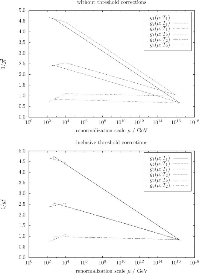
Refer to caption
Fig. 4: Running gauge couplings for parameter point PP1 for two different matching scales T1=500 GeVsubscript𝑇1times500gigaelectronvoltT_{1}=$500\text{\,}\mathrm{GeV}$ and T2=10 TeVsubscript𝑇2times10teraelectronvoltT_{2}=$10\text{\,}\mathrm{TeV}$ with and without threshold corrections.

As a test of this, Fig. 5 shows the E6SSM gauge couplings gi(Qfix)subscript𝑔𝑖subscript𝑄fixg_{i}(Q_{\text{fix}}) at the fixed scale Qfix=3 TeVsubscript𝑄fixtimes3teraelectronvoltQ_{\text{fix}}=$3\text{\,}\mathrm{TeV}$, as a function of the matching scale TE6SSMsubscript𝑇E6SSMT_{\text{E${}_{6}$SSM}} for parameter point PP1. In the case of the trivial matching relations (59) one finds a clear (unphysical) dependence of gi(Qfix)subscript𝑔𝑖subscript𝑄fixg_{i}(Q_{\text{fix}}) on TE6SSMsubscript𝑇E6SSMT_{\text{E${}_{6}$SSM}}. As shown in Eq. (12) the slopes of (4π)2/[2gi2(Qfix;TE6SSM)]superscript4𝜋2delimited-[]2superscriptsubscript𝑔𝑖2subscript𝑄fixsubscript𝑇E6SSM(4\pi)^{2}/[2g_{i}^{2}(Q_{\text{fix}};T_{\text{E${}_{6}$SSM}})] are given by the difference Δβi:=βiE6SSMβiSMassignΔsubscript𝛽𝑖superscriptsubscript𝛽𝑖E6SSMsuperscriptsubscript𝛽𝑖SM\Delta\beta_{i}:=\beta_{i}^{\text{E${}_{6}$SSM}}-\beta_{i}^{\text{SM}} of the one-loop gauge coupling beta functions, up to two-loop and iteration effects.
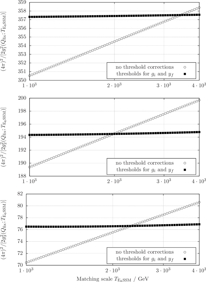
Refer to caption
Fig. 5: Dependency of the gauge couplings gisubscript𝑔𝑖g_{i} at Qfix=3 TeVsubscript𝑄fixtimes3teraelectronvoltQ_{\text{fix}}=$3\text{\,}\mathrm{TeV}$ on the matching scale TE6SSMsubscript𝑇E6SSMT_{\text{E${}_{6}$SSM}} for parameter point PP1. The circles show the behavior without threshold corrections and the squares with corrections for gisubscript𝑔𝑖g_{i} and yfsubscript𝑦𝑓y_{f}.

In Tab. 3, columns 4 and 5, the numerical values of ΔβiΔsubscript𝛽𝑖\Delta\beta_{i} as well as the slopes without threshold corrections for PP1 are listed. The values roughly coincide, thus confirming Eq. (12). When the threshold corrections (48), (49) and (32) are used, the matching scale dependency reduces to about 4 %times4percent4\text{\,}\% or less, resulting in the flattening of the curves shown in Fig. 5. The remaining matching scale dependency as well as the difference between columns 4 and 5 are due to still missing contributions of higher orders.

slopes of (4π)2/[2gi2(Qfix;TE6SSM)]superscript4𝜋2delimited-[]2superscriptsubscript𝑔𝑖2subscript𝑄fixsubscript𝑇E6SSM(4\pi)^{2}/[2g_{i}^{2}(Q_{\text{fix}};T_{\text{E${}_{6}$SSM}})]
Coupling βiE6SSMsubscriptsuperscript𝛽E6SSM𝑖\beta^{\text{E${}_{6}$SSM}}_{i} βiSMsubscriptsuperscript𝛽SM𝑖\beta^{\text{SM}}_{i} ΔβiΔsubscript𝛽𝑖\Delta\beta_{i} w/o thresh. w/ thresh.
g1subscript𝑔1g_{1} 9.69.69.6 4.14.14.1 5.55.55.5 5.675.675.67 0.180.180.18
g2subscript𝑔2g_{2} 444 3.173.17-3.17 7.177.177.17 7.427.427.42 0.320.320.32
g3subscript𝑔3g_{3} 00 77-7 777 7.337.337.33 0.290.290.29
slopes of (4π)2logyf(Qfix;TE6SSM)superscript4𝜋2subscript𝑦𝑓subscript𝑄fixsubscript𝑇E6SSM(4\pi)^{2}\log y_{f}(Q_{\text{fix}};T_{\text{E${}_{6}$SSM}})
βfE6SSM(TE6SSM)subscriptsuperscript𝛽E6SSM𝑓subscript𝑇E6SSM\beta^{\text{E${}_{6}$SSM}}_{f}(T_{\text{E${}_{6}$SSM}}) βfSM(TE6SSM)subscriptsuperscript𝛽SM𝑓subscript𝑇E6SSM\beta^{\text{SM}}_{f}(T_{\text{E${}_{6}$SSM}}) ΔβfΔsubscript𝛽𝑓-\Delta\beta_{f} w/o thresh. w/ thresh.
ytsubscript𝑦𝑡y_{t} 2.332.33-2.33 6.146.14-6.14 3.773.77-3.77 3.813.81-3.81 0.770.770.77
ybsubscript𝑦𝑏y_{b} 4.664.66-4.66 8.188.18-8.18 4.924.92-4.92 4.954.95-4.95 0.200.20-0.20
yτsubscript𝑦𝜏y_{\tau} 0.340.34-0.34 0.770.770.77 0.290.29-0.29 0.210.21-0.21 0.530.530.53
Tab. 3: Effect of the threshold corrections on the dependency of the gauge and Yukawa couplings on TE6SSMsubscript𝑇E6SSMT_{\text{E${}_{6}$SSM}} for parameter point PP1. The slopes in the last two columns are obtained by linear fits to the data in Fig. 5 and 6.

Fig. 6 shows the same analysis for the Yukawa couplings ytsubscript𝑦𝑡y_{t}, ybsubscript𝑦𝑏y_{b} and yτsubscript𝑦𝜏y_{\tau}. Analogous to the gauge couplings one expects the following slopes of the Yukawa couplings as a function of the matching scale

dlogyt(Qfix;t)dtdsubscript𝑦𝑡subscript𝑄fix𝑡d𝑡\displaystyle\frac{\mathrm{d}\log y_{t}(Q_{\text{fix}};t)}{\mathrm{d}t} =1(4π)2[βtE6SSM(t)βtSM(t)+βtanβ(t)cos2β]1(4π)2Δβt,absent1superscript4𝜋2delimited-[]superscriptsubscript𝛽𝑡E6SSM𝑡superscriptsubscript𝛽𝑡SM𝑡subscript𝛽𝛽𝑡superscript2𝛽1superscript4𝜋2Δsubscript𝛽𝑡\displaystyle=-\frac{1}{(4\pi)^{2}}\left[\beta_{t}^{\text{E${}_{6}$SSM}}(t)-\beta_{t}^{\text{SM}}(t)+\beta_{\tan\beta}(t)\cos^{2}\beta\right]\equiv-\frac{1}{(4\pi)^{2}}\Delta\beta_{t}, (65)
dlogyb,τ(Qfix;t)dtdsubscript𝑦𝑏𝜏subscript𝑄fix𝑡d𝑡\displaystyle\frac{\mathrm{d}\log y_{b,\tau}(Q_{\text{fix}};t)}{\mathrm{d}t} =1(4π)2[βb,τE6SSM(t)βb,τSM(t)βtanβ(t)sin2β]1(4π)2Δβb,τ.absent1superscript4𝜋2delimited-[]superscriptsubscript𝛽𝑏𝜏E6SSM𝑡superscriptsubscript𝛽𝑏𝜏SM𝑡subscript𝛽𝛽𝑡superscript2𝛽1superscript4𝜋2Δsubscript𝛽𝑏𝜏\displaystyle=-\frac{1}{(4\pi)^{2}}\left[\beta_{b,\tau}^{\text{E${}_{6}$SSM}}(t)-\beta_{b,\tau}^{\text{SM}}(t)-\beta_{\tan\beta}(t)\sin^{2}\beta\right]\equiv-\frac{1}{(4\pi)^{2}}\Delta\beta_{b,\tau}. (66)
Refer to caption
Fig. 6: Dependency of the Yukawa couplings yfsubscript𝑦𝑓y_{f} at Qfix=3 TeVsubscript𝑄fixtimes3teraelectronvoltQ_{\text{fix}}=$3\text{\,}\mathrm{TeV}$ on the matching scale TE6SSMsubscript𝑇E6SSMT_{\text{E${}_{6}$SSM}} for parameter point PP1. The circles show the behavior without threshold corrections and the squares with corrections for gisubscript𝑔𝑖g_{i} and yfsubscript𝑦𝑓y_{f}.

Note that these relations also contain the β𝛽\beta function for tanβ𝛽\tan\beta, defined in Eq. (D.14). In Tab. 3, columns 4 and 5, the numerical values of ΔβfΔsubscript𝛽𝑓\Delta\beta_{f} as well as the slopes without threshold corrections for PP1 are listed. One finds an agreement with the predicted slopes within a few percent. When the threshold corrections from Sec. 3.2 and 3.3 are taken into account one finds an overall reduction of the matching scale dependency effects. The remaining scale dependence is due to neglected higher-order effects, including in particular QED-logarithms of the small fermion masses in higher powers than taken into account in the one-loop computation of δmf𝛿subscript𝑚𝑓\delta m_{f} in Eqs. (50)–(52).

5.2 Particle masses

In softly broken SUSY models, like the CE6SSM, where the pattern of soft breaking masses is set substantially above the EW scale (e.g. MXsubscript𝑀𝑋M_{X}), the low-energy DR¯¯DR\overline{\text{DR}} running masses are very sensitive to the renormalization group flow of the gauge and Yukawa couplings. This implies that the physical mass spectrum strongly depends on the matching scale used for the gauge and Yukawa couplings unless stabilized by the inclusion of threshold corrections. Here we show how the inclusion of the CE6SSM threshold corrections improves the prediction of the low-energy DR¯¯DR\overline{\text{DR}} soft masses and yields a mass spectrum where the dependence on the unphysical matching scale is considerably reduced.

In Figs. 7 and 8 the dependency of the particle masses on the matching scale for parameter point PP1 is shown. The matching scale is varied in the range [12T0,2T0]12subscript𝑇02subscript𝑇0[\frac{1}{2}T_{0},2T_{0}], where T0=1.9 TeVsubscript𝑇0times1.9teraelectronvoltT_{0}=$1.9\text{\,}\mathrm{TeV}$ is the geometric average of all particle masses shown in Fig. 8.

Fig. 7 focuses on the gluino. The theory uncertainty implied by the TE6SSMsubscript𝑇E6SSMT_{\text{E${}_{6}$SSM}} dependence is 65 %times65percent65\text{\,}\% without threshold corrections (the percentage value is defined as the full variation of the particle mass divided by the mass at T0subscript𝑇0T_{0}). This huge uncertainty is entirely due to the missing threshold corrections, and including these reduces the uncertainty to only 0.5 %times0.5percent0.5\text{\,}\%.

Fig. 8 shows a subset of the generated particle spectrum for the parameter point PP1. The variation of the particle masses is drawn with a white box in case of trivial matching and with a black box in case of implemented threshold corrections. The gluino, the lightest chargino and the lightest neutralino show the biggest dependency with 65 %times65percent65\text{\,}\%, 83 %times83percent83\text{\,}\% and 85 %times85percent85\text{\,}\%, respectively.

Refer to caption
Fig. 7: Dependency of the gluino mass at Qfix=3 TeVsubscript𝑄fixtimes3teraelectronvoltQ_{\text{fix}}=$3\text{\,}\mathrm{TeV}$ on the matching scale TE6SSMsubscript𝑇E6SSMT_{\text{E${}_{6}$SSM}} for parameter point PP1. The circles show the behavior without threshold corrections and the squares with corrections for gisubscript𝑔𝑖g_{i} and yfsubscript𝑦𝑓y_{f}.

With the implemented threshold corrections, one finds a reduction of the variation down to 0.10.10.14 %times4percent4\text{\,}\%. The biggest decrease is found for the gluino, the lightest chargino and the lightest neutralino whose remaining variation is of the order of 0.5 %times0.5percent0.5\text{\,}\%. This is because the gluino mass is very sensitive to g3subscript𝑔3g_{3}, as can be seen from the RGEs of the soft parameter M3subscript𝑀3M_{3} [8]. Note that the remaining variation of the particle masses is due to 2-loop and iterative effects, which are of the order of up to 4 %times4percent4\text{\,}\%.

Refer to caption
Fig. 8: Particle spectra for parameter point PP1. The white and the black boxes show the variation of the particle masses when the matching scale TE6SSMsubscript𝑇E6SSMT_{\text{E${}_{6}$SSM}} is varied in the interval [12T0,2T0]12subscript𝑇02subscript𝑇0[\frac{1}{2}T_{0},2T_{0}], where T0=1.9 TeVsubscript𝑇0times1.9teraelectronvoltT_{0}=$1.9\text{\,}\mathrm{TeV}$ is the geometric average of all shown particle masses. The black boxes show the error with threshold corrections and the white boxes without.

Note that the variation of the matching scale is not always a good estimation of the theoretical uncertainty. For example the error band of mD~11subscript𝑚subscript~𝐷11m_{\tilde{D}_{11}} without threshold corrections in Fig. 8 is shifted when adding threshold corrections but is not reduced in size. As can be seen in Fig. 9 the reason for the shift is the non-linear behavior of mD~11subscript𝑚subscript~𝐷11m_{\tilde{D}_{11}} when TE6SSMsubscript𝑇E6SSMT_{\text{E${}_{6}$SSM}} is varied. In the interval [12T0,2T0]12subscript𝑇02subscript𝑇0[\frac{1}{2}T_{0},2T_{0}] the exotic mass mD~11subscript𝑚subscript~𝐷11m_{\tilde{D}_{11}} without threshold corrections happens to have a minimum which leads to an abnormally narrow error band. In contrast mD~21subscript𝑚subscript~𝐷21m_{\tilde{D}_{21}} shows the typical, approximately linear behavior in [12T0,2T0]12subscript𝑇02subscript𝑇0[\frac{1}{2}T_{0},2T_{0}] which leads to much better uncertainty estimation.
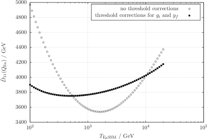
Refer to caption
Refer to caption
Fig. 9: Dependency of the first generation scalar exotic masses at Qfix=3 TeVsubscript𝑄fixtimes3teraelectronvoltQ_{\text{fix}}=$3\text{\,}\mathrm{TeV}$ on the matching scale TE6SSMsubscript𝑇E6SSMT_{\text{E${}_{6}$SSM}} for parameter point PP1. The circles show the behavior without threshold corrections and the squares with corrections for gisubscript𝑔𝑖g_{i} and yfsubscript𝑦𝑓y_{f}. In the interval [12T0,2T0]12subscript𝑇02subscript𝑇0[\frac{1}{2}T_{0},2T_{0}] the exotic mass mD~11subscript𝑚subscript~𝐷11m_{\tilde{D}_{11}} without threshold corrections has a minimum which leads to poor error estimation, whereas mD~21subscript𝑚subscript~𝐷21m_{\tilde{D}_{21}} is approximately linear within this interval.

5.3 Exploration of the E6SSM parameter space

5.3.1 Parameter space

We now turn from the specific benchmark point PP1 to a fuller investigation of the E6SSM parameter space. Since our main focus is the impact of threshold corrections we still restrict ourselves to a two-dimensional slice of the 121212-dimensional parameter space. We choose to keep the Yukawa couplings of the SU(5)𝑆𝑈5SU(5) 555-plets containing H^1isubscript^𝐻1𝑖\hat{H}_{1i}, H^2isubscript^𝐻2𝑖\hat{H}_{2i}, D^isubscript^𝐷𝑖\hat{D}_{i} and barD^isubscript^bar𝐷𝑖\hat{\mathrm{bar}{D}}_{i} the same and generation-independent, thus leaving a single unified exotic Yukawa coupling, defined at the GUT scale MXsubscript𝑀𝑋M_{X},

λ1=λ2=λ3=κ1=κ2=κ3subscript𝜆1subscript𝜆2subscript𝜆3subscript𝜅1subscript𝜅2subscript𝜅3\displaystyle\lambda_{1}=\lambda_{2}=\lambda_{3}=\kappa_{1}=\kappa_{2}=\kappa_{3} (67)

between those states and the third generation singlet. In addition we fix

s=μ=mH=mbarH=10 TeV,Bμ=0.formulae-sequence𝑠superscript𝜇subscript𝑚superscript𝐻subscript𝑚barsuperscript𝐻times10teraelectronvolt𝐵superscript𝜇0\displaystyle s=\mu^{\prime}=m_{H^{\prime}}=m_{\mathrm{bar}{H^{\prime}}}=$10\text{\,}\mathrm{TeV}$,B\mu^{\prime}=0. (68)

The remaining input parameters are tanβ𝛽\tan\beta and λ3subscript𝜆3\lambda_{3}, and we scan over them in the range

tanβ[2,45],λ3[0,3].formulae-sequence𝛽245subscript𝜆303\displaystyle\tan\beta\in[2,45],\qquad\lambda_{3}\in[0,3]. (69)

Note that we are defining λ3subscript𝜆3\lambda_{3} at the GUT scale, and in this respect the numerical value should not be compared with λ𝜆\lambda in the NMSSM which is often defined near the electroweak scale (EW). By defining λ3subscript𝜆3\lambda_{3} at the GUT scale we ensure automatically that it is perturbative at all scales between the electroweak and the GUT scale.666In the NMSSM it is well known that to ensure perturbativity λ(EW)0.7less-than-or-similar-to𝜆EW0.7\lambda(\text{EW})\lesssim 0.7, while an analysis of this in the E6SSM [2] found that λ3(EW)0.85less-than-or-similar-tosubscript𝜆3EW0.85\lambda_{3}(\text{EW})\lesssim 0.85 is required for perurbativity up to the GUT scale, though this limit depends on the values of the other exotic Yukawa couplings and tanβ𝛽\tan\beta.

For each choice of (tanβ,λ3)𝛽subscript𝜆3(\tan\beta,\lambda_{3}), requiring electroweak symmetry breaking simultaneously with (68) leads to up to four solutions for (m0,M1/2)subscript𝑚0subscript𝑀12(m_{0},M_{1/2}), which we number consecutively. In the following (m0,M1/2)subscript𝑚0subscript𝑀12(m_{0},M_{1/2})-plots we will show all of them, where solution 1 is preferred over solution 2 in the overlap region. In Figs. 1819 we will show only the first solution for simplicity.

Since our input parameters (tanβ,λ3)𝛽subscript𝜆3(\tan\beta,\lambda_{3}) have less direct physical meaning than the output parameters (m0,M1/2)subscript𝑚0subscript𝑀12(m_{0},M_{1/2}), we display many results in the (m0,M1/2)subscript𝑚0subscript𝑀12(m_{0},M_{1/2}) plane. To better understand the connection between these two sets we show in Fig. 10 the mapping of (tanβ,λ3)(m0,M1/2)𝛽subscript𝜆3subscript𝑚0subscript𝑀12(\tan\beta,\lambda_{3})\rightarrow(m_{0},M_{1/2}). In the top panel we show as a color contour plot how tanβ𝛽\tan\beta varies over the (m0,M1/2)subscript𝑚0subscript𝑀12(m_{0},M_{1/2}) plane, while on the lower plot we do the same for λ3subscript𝜆3\lambda_{3}. Fig. 10 thus allows to read off the original input values for (tanβ,λ3)𝛽subscript𝜆3(\tan\beta,\lambda_{3}) for any given point in the subsequent plots.

The butterfly shape of Fig. 10 is due to the superposition of the four solutions. Most of the (m0,M1/2)subscript𝑚0subscript𝑀12(m_{0},M_{1/2}) space is covered by relatively small λ3<0.4subscript𝜆30.4\lambda_{3}<0.4, while larger values of lambda are concentrated in a narrow region of the parameter space due to the renormalisation group flow leading to a focusing on a significantly smaller range of λ3subscript𝜆3\lambda_{3} at the electroweak scale. The tanβ𝛽\tan\beta dependency depends on the solution, but in much of the parameter space large values of tanβ𝛽\tan\beta are associated with large m0subscript𝑚0m_{0} and small M1/2subscript𝑀12M_{1/2}.

Fig. 10 is not exactly symmetric in ±M1/2plus-or-minussubscript𝑀12\pm M_{1/2} because λ3subscript𝜆3\lambda_{3} and therefore the effective μ𝜇\mu-parameter is required to be positive in our analysis.
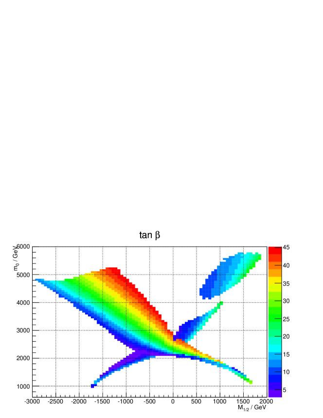
Refer to caption
Refer to caption
Fig. 10: Illustration of the mapping (tanβ,λ3)(m0,M1/2)𝛽subscript𝜆3subscript𝑚0subscript𝑀12(\tan\beta,\lambda_{3})\rightarrow(m_{0},M_{1/2}). The top panel shows the input parameter tanβ𝛽\tan\beta varying across the (m0,M1/2)subscript𝑚0subscript𝑀12(m_{0},M_{1/2}) plane (of output parameters). The bottom panel shows the same for the input parameter λ3subscript𝜆3\lambda_{3}.

5.3.2 Experimental constraints

At this point we briefly summarize the various experimental constraints on the model. A more detailed discussion can be found in [10].

Since the publication of the first studies of the CE6SSM [8, 9] the Atlas and CMS experiments have already placed strong constraints on supersymmetry from the first 5 fb1absentsuperscripttimes5femtobarn1\approx$5\text{\,}\mathrm{fb}$^{-1} of data gathered from the LHC running at s=7 TeV𝑠times7teraelectronvolt\sqrt{s}=$7\text{\,}\mathrm{TeV}$. With 4.7 fb1superscripttimes4.7femtobarn1$4.7\text{\,}\mathrm{fb}$^{-1} of data Atlas have performed searches for squarks and gluinos, by looking for jets plus missing transverse momentum and possibly one isolated lepton [43, 44, 45] and presented the constraints in a CMSSM interpretation.777They also presented constraints in a simplified model interpretation, however this is less relevant for our present purposes since the physical spectrum of our model, especially if the colored exotics are heavy, is far closer to that of the CMSSM than the simplified models. CMS collaboration have also placed similar constraints using the razor analysis [46] with 4.4 fb1superscripttimes4.4femtobarn1$4.4\text{\,}\mathrm{fb}$^{-1} of data [47] and another analysis with the transverse mass variable [48] using 4.73 fb1superscripttimes4.73femtobarn1$4.73\text{\,}\mathrm{fb}$^{-1} of data. Very recently the ATLAS released updated results with 5.8 fb1superscripttimes5.8femtobarn1$5.8\text{\,}\mathrm{fb}$^{-1} data from the s=8 TeV𝑠times8teraelectronvolt\sqrt{s}=$8\text{\,}\mathrm{TeV}$ run [49].

It was estimated in [50, 10] that the effect of these constraints on the CE6SSM is to place a limit on the gluino mass, close to 850 GeVtimes850gigaelectronvolt850\text{\,}\mathrm{GeV}. Since the squarks must always be heavier than the gluino, due to the RG flow,888The soft scalar masses get large contributions (relative to the gauginos) from M1/2subscript𝑀12M_{1/2}, due to the renormalization group evolution, which is very different from the MSSM case. squark limits are automatically satisfied. However the 888 TeV data has increased the limits on the gluino, in the heavy squarks region the limit varies between 900absent900\approx 900100010001000 GeV.

However it is also of interest to point out that in certain E6SSM scenarios (where the bino-like neutralino is not stable, leading to longer cascade decays and an alternative LSP) the gluino limits from these searches may not apply [18] resulting in different limits.

Furthermore, there are limits on the Higgs mass [51, 52] from analyses using between 4.64.64.6 and 4.9 fb1superscripttimes4.9femtobarn1$4.9\text{\,}\mathrm{fb}$^{-1} of LHC data. At 95 %times95percent95\text{\,}\% confidence level Atlas exclude a standard model Higgs in the ranges 110.0110.0110.0117.5 GeVtimes117.5gigaelectronvolt117.5\text{\,}\mathrm{GeV}, 118.5118.5118.5122.5 GeVtimes122.5gigaelectronvolt122.5\text{\,}\mathrm{GeV} and 129129129539 GeVtimes539gigaelectronvolt539\text{\,}\mathrm{GeV}, while at the same confidence level CMS exclude 127.5127.5127.5600 GeVtimes600gigaelectronvolt600\text{\,}\mathrm{GeV}. This leaves a narrow allowed window of 117.5117.5117.5118.5 GeVtimes118.5gigaelectronvolt118.5\text{\,}\mathrm{GeV} and a wider one of 123.5123.5123.5127.5 GeVtimes127.5gigaelectronvolt127.5\text{\,}\mathrm{GeV}.

As this paper was being finalized the discovery of a new particle consistent with a Higgs boson with a mass of around 125125125126 GeVtimes126gigaelectronvolt126\text{\,}\mathrm{GeV} was announced by ATLAS [28] and CMS [29]. CMS report a 5.0σ5.0𝜎5.0\sigma excess at 125.5 GeVtimes125.5gigaelectronvolt125.5\text{\,}\mathrm{GeV} and quote a best fit mass of 125.3±0.4(stat.)±0.5(syst.)plus-or-minus125.30.4(stat.)0.5(syst.)125.3\pm 0.4\text{(stat.)}\pm 0.5\text{(syst.)} GeV while ATLAS find a 6.0σ6.0𝜎6.0\sigma excess at 126.5126.5126.5, and using the two channels with the highest mass resolution estimate the mass as 126.0±0.4(stat.)±0.4(syst.)plus-or-minus126.00.4(stat.)0.4(syst.)126.0\pm 0.4\text{(stat.)}\pm 0.4\text{(syst.)} GeV.

The strongest current constraint on the ZNsubscriptsuperscript𝑍𝑁Z^{\prime}_{N} comes from a CMS analysis using 5 fb1absentsuperscripttimes5femtobarn1\approx$5\text{\,}\mathrm{fb}$^{-1} of data [53], announced as this paper is being finalized and setting a lower limit of 2.08 TeVtimes2.08teraelectronvolt2.08\text{\,}\mathrm{TeV} on the mass of the ZNsubscriptsuperscript𝑍𝑁Z^{\prime}_{N} boson. However one should note that the lower limit assumes there are now light exotics available for the Zsuperscript𝑍Z^{\prime} to decay into. If such are present then the branching ratio to leptons is diluted and the limits are weaker.

Finally the model also contains exotic (colored and inert) fermions and sfermions. The inert states are weakly produced and we do not anticipate very large new limits to be set by the early data from the LHC, but the colored states should be produced abundantly and could be tightly constrained. However the existing analyses do not apply to the fermionic diquarks or leptoquarks described in this model since they carry half integer spin and are odd under their respective discrete symmetries, decaying with missing energy. Thus it is currently unknown what limit the LHC has placed on their mass. Here we will only consider cases where these exotics are heavy anyway but when discussing existing benchmarks from the literature we will not apply any new constraints on them.

The E6SSM also contains a number of dark matter candidates. It is possible that the correct relic density can be achieved entirely from the inert sector neutralinos (admixtures of inert singlinos and inert higgsinos) [54] however such a scenario is now in conflict with XENON-100 limits [55] though if one allows for a relic density which is too small to explain observations (and therefore would require some additional contributions to dark matter) consistency could be achieved. Alternatively another possible scenario described in Ref. [56] is that there is a large splitting between the inert states with one at a few keV and another a few GeV, thus giving warm dark matter scenarios, which match observation. For cases studied the couplings which are assumed to be negligible here are too large to avoid perturbing the RG evolution and may be too large for consistency with the constrained model generally. However such scenarios have only recently been proposed and the full parameters space far from explored so it is simply unknown whether or not this could be applied with couplings which would be consistent with the scenarios explored here.

A third possibility which is known to be consistent with the constrained version of the model decouples the singlinos from the rest of the spectrum, giving a new contribution to the effective number of neutrinos (which is consistent with observation) [57]. The bino is then the dark matter candidate, but the scenario is still very distinct from typical models with bino dominated dark matter because the inert Higgsinos play a crucial role in enabling the correct relic density to be achieved so long as the mass of the lightest inert neutralino is related to that of the lightest neutralino by the condition [57],

μH~1|mχ~10|+10 GeV.subscript𝜇subscript~𝐻1subscript𝑚superscriptsubscript~𝜒10times10gigaelectronvolt\displaystyle\mu_{\tilde{H}_{1}}\approx|m_{\tilde{\chi}_{1}^{0}}|+$10\text{\,}\mathrm{GeV}$. (70)

In the scans we perform here we do not explicitly satisfy this constraint (and instead our inert Higgsinos are typically far heavier) as we assume a universality amongst all exotic Yukawa couplings. Splitting one generation of all exotics or just inerts could solve this problem. Doing so would perturb the renormalization group equations and distort the parameter space somewhat, though the qualitative results and understanding of the impact that these thresholds can have would not be altered. Alternatively one can keep in mind the “keVins and GeVins” scenarios though it is currently unknown if this could result in the correct relic density or not.

5.3.3 Change in masses from threshold corrections

Now we look at the significance of the threshold effects throughout the parameter space described in Sec. 5.3.1. Like for the point PP1, the largest corrections are observed in the gaugino sector for states whose masses are set by M1/2subscript𝑀12M_{1/2}. Fig. 11 shows the shifts in mass for the gluino and lightest neutralino in the (m0,M1/2)subscript𝑚0subscript𝑀12(m_{0},M_{1/2})-plane.999Note that these are the m0subscript𝑚0m_{0} and M1/2subscript𝑀12M_{1/2} values obtained from the spectrum generator when thresholds are included. Since m0subscript𝑚0m_{0} and M1/2subscript𝑀12M_{1/2} are outputs they are affected by the threshold corrections and so do not match the values for the point without threshold corrections. We compare between results with trivial matching conditions to those with full threshold corrections, where in both cases the matching scale used is the “optimal” choice, where TE6SSMsubscript𝑇E6SSMT_{\text{E${}_{6}$SSM}} is set to the geometric average of the particle masses.
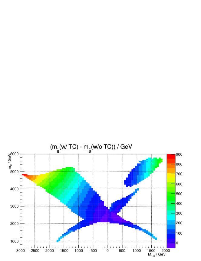
Refer to caption
Refer to caption
Fig. 11: Change in the gluino and in the lightest neutralino mass when adding threshold corrections for s=μ=mH=mbarH=10 TeV𝑠superscript𝜇subscript𝑚superscript𝐻subscript𝑚barsuperscript𝐻times10teraelectronvolts=\mu^{\prime}=m_{H^{\prime}}=m_{\mathrm{bar}{H^{\prime}}}=$10\text{\,}\mathrm{TeV}$, tanβ[2,45]𝛽245\tan\beta\in[2,45] and λi(MX)=κi(MX)[0,3]subscript𝜆𝑖subscript𝑀𝑋subscript𝜅𝑖subscript𝑀𝑋03\lambda_{i}(M_{X})=\kappa_{i}(M_{X})\in[0,3].

We show the absolute change in masses rather than relative change because, when the masses are light due to a cancellation, the relative corrections can be very large, distorting the plot. However it is important to note that the gaugino masses though not shown can be estimated since the low-energy soft gaugino masses Misubscript𝑀𝑖M_{i} (which give the dominant contribution to mg~subscript𝑚~𝑔m_{\tilde{g}} and mχ~10subscript𝑚superscriptsubscript~𝜒10m_{\tilde{\chi}_{1}^{0}}) are proportional M1/2subscript𝑀12M_{1/2}, with mg~0.85M1/2similar-tosubscript𝑚~𝑔0.85subscript𝑀12m_{\tilde{g}}\sim 0.85M_{1/2}, mχ~100.15M1/2similar-tosubscript𝑚superscriptsubscript~𝜒100.15subscript𝑀12m_{\tilde{\chi}_{1}^{0}}\sim 0.15M_{1/2}. Fig. 12 shows the actual gluino and neutralino masses after including threshold corrections for comparison.
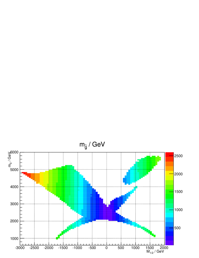
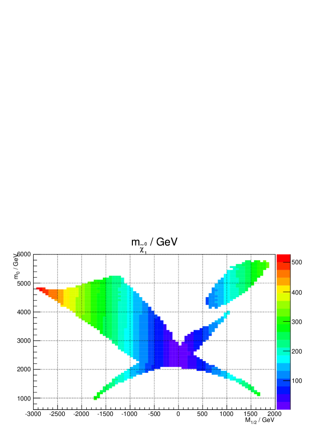
Refer to caption
Refer to caption
Fig. 12: Gluino and in the lightest neutralino mass as a function of M1/2subscript𝑀12M_{1/2} and m0subscript𝑚0m_{0}, where it was varied tanβ[3,50]𝛽350\tan\beta\in[3,50], λi=κi[0,3]subscript𝜆𝑖subscript𝜅𝑖03\lambda_{i}=\kappa_{i}\in[0,3], s=10 TeV𝑠times10teraeVs=$10\text{\,}\mathrm{T}$\mathrm{eV}, μ=mH=mbarH=10 TeVsuperscript𝜇subscript𝑚superscript𝐻subscript𝑚barsuperscript𝐻times10teraeV\mu^{\prime}=m_{H^{\prime}}=m_{\mathrm{bar}{H^{\prime}}}=$10\text{\,}\mathrm{T}$\mathrm{eV}.

Once again we see substantial changes in both the gluino and neutralino mass across a wide range of the parameter space with corrections being small only in a very narrow region of the space. Around the LHC limit on gluinos we can see there can be large corrections of the order of several 100 GeVtimes100gigaelectronvolt100\text{\,}\mathrm{GeV} for the gluino mass, therefore these corrections can make a significant impact in determining whether or not a point is ruled out by LHC search constraints. The corrections to the gluino mass can be positive or negative, depending on whether the masses appearing in the logarithmic corrections are larger or smaller than the threshold scale.101010In this case the dominant corrections arise from corrections to g3subscript𝑔3g_{3}, see Eq. (32).

The corrections to the neutralino are also substantial, varying from just below zero to just over 200200200 GeV. They are distinctly correlated with the corrections to the gluino, showing close to identical variation, which is because the dominant effect is a shift in M1/2subscript𝑀12M_{1/2}.

Refer to caption
Fig. 13: Change in the lightest CP even Higgs mass when adding threshold corrections for s=μ=mH=mbarH=10 TeV𝑠superscript𝜇subscript𝑚superscript𝐻subscript𝑚barsuperscript𝐻times10teraelectronvolts=\mu^{\prime}=m_{H^{\prime}}=m_{\mathrm{bar}{H^{\prime}}}=$10\text{\,}\mathrm{TeV}$, tanβ[2,45]𝛽245\tan\beta\in[2,45] and λi(MX)=κi(MX)[0,3]subscript𝜆𝑖subscript𝑀𝑋subscript𝜅𝑖subscript𝑀𝑋03\lambda_{i}(M_{X})=\kappa_{i}(M_{X})\in[0,3]. We show only points where the change is less than 5 GeVtimes5gigaelectronvolt5\text{\,}\mathrm{GeV}.

With the recent discovery of a Higgs-like boson [28, 29] with a mass 125absent125\approx 125126126126 GeV and strong constraints on a SM-like Higgs away from the mass of this new state, the lightest Higgs mass is a crucial observable in constraining the parameter space of SUSY models. The corrections to the lightest Higgs mass from threshold effects are not expected to be very large since it’s mass is not set by soft mass parameters at tree level. However even small corrections to the Higgs mass can significantly shift the m0subscript𝑚0m_{0} and M1/2subscript𝑀12M_{1/2} values which a particular Higgs mass is compatible with and this can dramatically alter how the Higgs mass measurement combines with the constraints coming from squark and gluino searches.
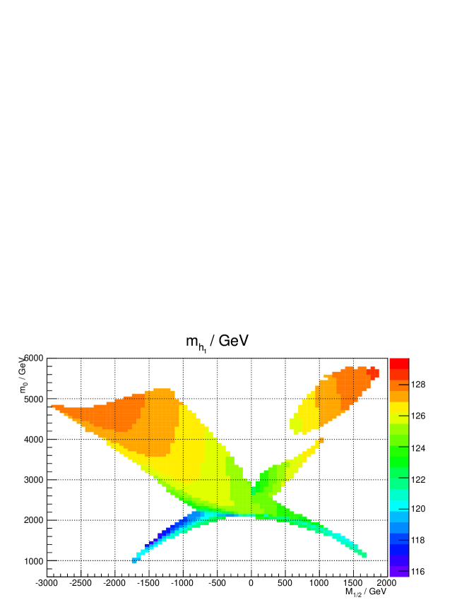
Refer to caption
Fig. 14: Lightest CP even Higgs mass mh1subscript𝑚subscript1m_{h_{1}} as a function of M1/2subscript𝑀12M_{1/2} and m0subscript𝑚0m_{0}, where it was varied tanβ[3,50]𝛽350\tan\beta\in[3,50], λi=κi[0,3]subscript𝜆𝑖subscript𝜅𝑖03\lambda_{i}=\kappa_{i}\in[0,3], s=10 TeV𝑠times10teraeVs=$10\text{\,}\mathrm{T}$\mathrm{eV}, μ=mH=mbarH=10 TeVsuperscript𝜇subscript𝑚superscript𝐻subscript𝑚barsuperscript𝐻times10teraeV\mu^{\prime}=m_{H^{\prime}}=m_{\mathrm{bar}{H^{\prime}}}=$10\text{\,}\mathrm{T}$\mathrm{eV}.

In Fig. 13 the corrections to the Higgs mass are shown across the (m0,M1/2)subscript𝑚0subscript𝑀12(m_{0},M_{1/2})-plane. The corrections vary between around 0.70.7-0.7 GeV to +1.71.7+1.7 GeV. One can also see in Fig. 14 the Higgs mass itself and note that for the parameter set studied here the Higgs mass is consistent with the new particle discovered by ATLAS and CMS in the large m0subscript𝑚0m_{0} and M1/2subscript𝑀12M_{1/2} regions of the parameter space where the corrections from the thresholds are largest.

5.3.4 Allowed parameter space

With the more reliable predictions at hand, we turn to understanding the overall allowed region of parameter space. Dominant experimental constraints come from the gluino and the Higgs, see Figs. 12 and 14. We can see that for our choice of s𝑠s the gluino is comfortably above the LHC limit in a large volume the parameter space. In the Higgs contour plot Fig. 14 we also see a very large volume of the parameter space where the light Higgs mass is within the narrow window on it’s allowed mass from the LHC discovery. Nevertheless in fact the combination of the two constraints creates very stringent limits of this slice of the parameter space.

To show the impact more precisely we now plot in Fig. 15 the valid and invalid parameter space including all relevant constraints, both in terms of (tanβ,λ3)𝛽subscript𝜆3(\tan\beta,\lambda_{3}) and of (m0,M1/2)subscript𝑚0subscript𝑀12(m_{0},M_{1/2}). While it is beyond the scope of the current project to take account of full experimental likelihoods or include precise 959595% confidence limit contours, to provide a guide as to the parameter space which evades LHC constraints we define valid points as those satisfying,

123.5 GeV<mh1<127.5 GeV,times123.5gigaelectronvoltsubscript𝑚subscript1times127.5gigaelectronvolt\displaystyle$123.5\text{\,}\mathrm{GeV}$<m_{h_{1}}<$127.5\text{\,}\mathrm{GeV}$, (71)
mg~>1 TeV,subscript𝑚~𝑔times1teraelectronvolt\displaystyle m_{\tilde{g}}>$1\text{\,}\mathrm{TeV}$, (72)
mt~1>300 GeV,subscript𝑚subscript~𝑡1times300gigaelectronvolt\displaystyle m_{\tilde{t}_{1}}>$300\text{\,}\mathrm{GeV}$, (73)
mχ~10,mχ~1±>200 GeV,subscript𝑚superscriptsubscript~𝜒10subscript𝑚superscriptsubscript~𝜒1plus-or-minustimes200gigaelectronvolt\displaystyle m_{\tilde{\chi}_{1}^{0}},m_{\tilde{\chi}_{1}^{\pm}}>$200\text{\,}\mathrm{GeV}$, (74)
mZ>2.1 TeV,subscript𝑚superscript𝑍times2.1teraelectronvolt\displaystyle m_{Z^{\prime}}>$2.1\text{\,}\mathrm{TeV}$, (75)
mh~li0,mh~i+,mhij0,mhij±>100 GeV,subscript𝑚superscriptsubscript~𝑙𝑖0subscript𝑚superscriptsubscript~𝑖subscript𝑚superscriptsubscript𝑖𝑗0subscript𝑚superscriptsubscript𝑖𝑗plus-or-minustimes100gigaelectronvolt\displaystyle m_{\tilde{h}_{li}^{0}},m_{\tilde{h}_{i}^{+}},m_{h_{ij}^{0}},m_{h_{ij}^{\pm}}>$100\text{\,}\mathrm{GeV}$, (76)

which are based on the discussion of Sec. 5.3.2.

One finds that the lower bound on mg~subscript𝑚~𝑔m_{\tilde{g}} and the bounds on mh1subscript𝑚subscript1m_{h_{1}} are most constraining. This is because the gluino is driven lighter than the sfermions by the renormalization group flow with, M30.7M1/2200similar-tosubscript𝑀30.7subscript𝑀12similar-to200M_{3}\sim 0.7M_{1/2}\sim 2001400 GeVtimes1400gigaelectronvolt1400\text{\,}\mathrm{GeV}, while for the Higgs we now have a very narrow range of allowed masses as a result of Higgs searches that ultimately lead to the recent discovery. Here we find the lightest Higgs mass is around mh1118similar-tosubscript𝑚subscript1118m_{h_{1}}\sim 118128 GeVtimes128gigaelectronvolt128\text{\,}\mathrm{GeV} [8], as shown in Fig. 14, including a substantial region of parameter space where the CE6SSM predicts a lightest Higgs with a mass of 123.5123.5123.5127.5 GeVtimes127.5gigaelectronvolt127.5\text{\,}\mathrm{GeV}, consistent with the discovery.

Refer to caption
Fig. 15: Exclusion plot of the E6SSM parameter space.

While the allowed region appears strongly restricted in (tanβ,λ3)𝛽subscript𝜆3(\tan\beta,\lambda_{3})-space, it appears reasonably large in the (m0,M1/2)subscript𝑚0subscript𝑀12(m_{0},M_{1/2})-plane. The reason is the non-trivial mapping between these two spaces, as illustrated by Fig. 10. The valid green region in the (tanβ,λ3)𝛽subscript𝜆3(\tan\beta,\lambda_{3})-space of Fig. 15 is mapped onto different wings of the butterfly in the (m0,M1/2)subscript𝑚0subscript𝑀12(m_{0},M_{1/2})-plane.

Fig. 15 also shows that even without imposing experimental constraints there are upper and lower limits on all the parameters. Outside the colored regions no simultaneous solution to electroweak symmetry breaking and unification without tachyonic masses can be found. In particular, there is an upper limit on tanβ𝛽\tan\beta at around 454545. Here the EWSB minima become unstable giving a tachyonic Higgs mass, as shown in Fig. 16 for both the uncorrected Higgs mass and for the threshold corrected value, which converge in this region.
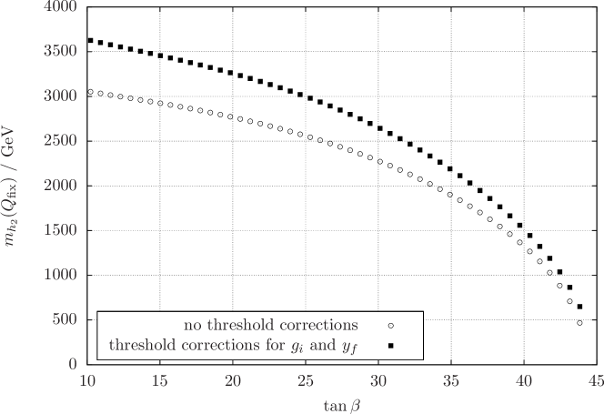
Refer to caption
Fig. 16: Second lightest CP even Higgs mass as a function of tanβ𝛽\tan\beta for s=μ=mH=mbarH=10 TeV𝑠superscript𝜇subscript𝑚superscript𝐻subscript𝑚barsuperscript𝐻times10teraelectronvolts=\mu^{\prime}=m_{H^{\prime}}=m_{\mathrm{bar}{H^{\prime}}}=$10\text{\,}\mathrm{TeV}$ and λi(MX)=κi(MX)=0.2subscript𝜆𝑖subscript𝑀𝑋subscript𝜅𝑖subscript𝑀𝑋0.2\lambda_{i}(M_{X})=\kappa_{i}(M_{X})=0.2

At such large tanβ𝛽\tan\beta the bottom quark Yukawa coupling is much closer to the top quark Yukawa coupling, and in such a situation generating a large splitting between the Higgs masses required for correct EWSB is difficult. A simple tree-level condition for keeping mA2>0superscriptsubscript𝑚𝐴20m_{A}^{2}>0 at large tanβ𝛽\tan\beta can be derived in the MSSM [58] and in the E6SSM,

MSSM: mHd2mHu2MSSM: superscriptsubscript𝑚subscript𝐻𝑑2superscriptsubscript𝑚subscript𝐻𝑢2\displaystyle\mbox{MSSM: }m_{H_{d}}^{2}-m_{H_{u}}^{2} mZ2,greater-than-or-equivalent-toabsentsuperscriptsubscript𝑚𝑍2\displaystyle\gtrsim m_{Z}^{2}, (77)
E6SSM: mHd2mHu2E6SSM: superscriptsubscript𝑚subscript𝐻𝑑2superscriptsubscript𝑚subscript𝐻𝑢2\displaystyle\mbox{E\textsubscript{6}SSM: }m_{H_{d}}^{2}-m_{H_{u}}^{2} mZ2+gN24ΣQ(NH2NH1).greater-than-or-equivalent-toabsentsuperscriptsubscript𝑚𝑍2superscriptsubscript𝑔𝑁24subscriptΣ𝑄subscript𝑁subscript𝐻2subscript𝑁subscript𝐻1\displaystyle\gtrsim m_{Z}^{2}+\frac{g_{N}^{2}}{4}\Sigma_{Q}(N_{H_{2}}-N_{H_{1}}). (78)

The E6SSM condition is stricter since it contains an additional positive term involving,111111The term is positive so long as s>v𝑠𝑣s>v, which is always the case due to limits on the Zsuperscript𝑍Z^{\prime} mass.

ΣQ=12(NH1v12+NH2v22+NSs2).subscriptΣ𝑄12subscript𝑁subscript𝐻1superscriptsubscript𝑣12subscript𝑁subscript𝐻2superscriptsubscript𝑣22subscript𝑁𝑆superscript𝑠2\displaystyle\Sigma_{Q}=\frac{1}{2}(N_{H_{1}}v_{1}^{2}+N_{H_{2}}v_{2}^{2}+N_{S}s^{2}). (79)

5.4 Dependency on the survival Higgs parameters

The inclusion of threshold corrections not only reduces the unphysical matching-scale dependence. It also leads to a physical dependence on the survival Higgs sector. Without thresholds the spectrum does not explicitly depend on the survival Higgs masses as the renormalization group equations decouple. With threshold corrections the survival Higgs parameters appear in the threshold corrections to the gauge couplings, and thus affect both gauge coupling unification and the low-energy mass spectrum. We will now study these two aspects in a simplified setting by taking a single scale

msurvμ=mH=mbarH.subscript𝑚survsuperscript𝜇subscript𝑚superscript𝐻subscript𝑚barsuperscript𝐻\displaystyle m_{\text{surv}}\equiv\mu^{\prime}=m_{H^{\prime}}=m_{\mathrm{bar}{H^{\prime}}}. (80)

Figs. 17 and 18 focus on gauge-coupling unification. We recall that in our approach MXsubscript𝑀𝑋M_{X} is defined by the intersection of g1subscript𝑔1g_{1} and g2subscript𝑔2g_{2}, while g3subscript𝑔3g_{3} is determined by its running from its low-energy measured value. Fig. 17 shows that for the parameter choice PP1, exact unification can be achieved by adjusting msurv=200 GeVsubscript𝑚survtimes200gigaelectronvoltm_{\text{surv}}=$200\text{\,}\mathrm{GeV}$, while e.g. msurv=16 TeVsubscript𝑚survtimes16teraeVm_{\text{surv}}=$16\text{\,}\mathrm{T}$\mathrm{eV} leads to a substantial deviation between g3subscript𝑔3g_{3} and g2subscript𝑔2g_{2} at the GUT scale.

Refer to caption
Fig. 17: Splitting between g1subscript𝑔1g_{1} and g3subscript𝑔3g_{3} at MXsubscript𝑀𝑋M_{X} for two different choices of msurvsubscript𝑚survm_{\text{surv}} for PP1.

Of course in a full GUT model there will be GUT scale threshold corrections. Nevertheless Fig. 17 makes clear that requiring a precise splitting between the gauge couplings from any given GUT threshold correction will fix the survival Higgs scale.

Fig. 18 shows gauge coupling (non-)unification for the entire parameter space defined by Eqs. (67)–(69) except that tanβ=10𝛽10\tan\beta=10 is fixed and msurvsubscript𝑚survm_{\text{surv}} is varied in the range

msurv[0.1,1000]TeV.subscript𝑚surv0.11000TeV\displaystyle m_{\text{surv}}\in[0.1,1000]\;\mathrm{T}\mathrm{eV}. (81)

Like in Fig. 17, we find that the deviation (g1g3)subscript𝑔1subscript𝑔3(g_{1}-g_{3}) at MXsubscript𝑀𝑋M_{X} depends substantially on the survival Higgs masses, and for any given lambda there is a survival Higgs scale which allows exact unification or any splitting required by GUT thresholds between 00 and O(0.1)𝑂0.1O(0.1).

Refer to caption
Fig. 18: Splitting between g1subscript𝑔1g_{1} and g3subscript𝑔3g_{3} at MXsubscript𝑀𝑋M_{X} in the (λ3,msurv)subscript𝜆3subscript𝑚surv(\lambda_{3},m_{\text{surv}}) parameter space

Figs. 19 and 20 focus on the influence of msurvsubscript𝑚survm_{\text{surv}} on the mass spectrum. In Fig. 19 we plot the variation of the gluino mass across the (msurv,λ3)subscript𝑚survsubscript𝜆3(m_{\text{surv}},\lambda_{3})-plane and see that the dependence on the survival Higgs masses is extremely weak. The figure also shows that the lightest neutralino mass is affected slightly more, in particular in regions where it is rather heavy (250similar-toabsent250\sim 250300 GeVtimes300gigaelectronvolt300\text{\,}\mathrm{GeV}).

Refer to caption
Refer to caption
Fig. 19: Gluino mass mg~subscript𝑚~𝑔m_{\tilde{g}} and mass of the lightest neutralino mχ~10subscript𝑚subscriptsuperscript~𝜒01m_{\tilde{\chi}^{0}_{1}} in the (λ3,msurv)subscript𝜆3subscript𝑚surv(\lambda_{3},m_{\text{surv}}) parameter space

Typically the survival Higgses and Higgsinos are too heavy to be observed at the LHC, since they are only weakly produced and have the couplings of a 4th generation lepton with current mass limit on the mass of 100.8 GeVtimes100.8gigaelectronvolt100.8\text{\,}\mathrm{GeV}.

For cases where they are not observable and where we do not constrain the splitting between the gauge couplings at the GUT scale, we can therefore consider them as an additional error in the theoretical calculation. This is the approach we now take here. To look at this in detail we again turn to our test case PP1.

Fig. 20 shows the dependency of the particle spectrum on the new model parameter msurvsubscript𝑚survm_{\text{surv}} for PP1. It is instructive to compare the result to Fig. 8, where the sensitivity to the matching scale TE6SSMsubscript𝑇E6SSMT_{\text{E${}_{6}$SSM}} with and without threshold corrections is shown. In the comparison one has to bear in mind that the msurvsubscript𝑚survm_{\text{surv}}-dependence is physical and that we vary msurvsubscript𝑚survm_{\text{surv}} in a much larger interval than TE6SSMsubscript𝑇E6SSMT_{\text{E${}_{6}$SSM}}.

One finds a significant msurvsubscript𝑚survm_{\text{surv}}-dependence only for masses which were also strongly sensitive to the choice of matching scale without threshold corrections. This is because a variation of TE6SSMsubscript𝑇E6SSMT_{\text{E${}_{6}$SSM}} changes the size of all the logarithmic contributions to the threshold corrections, while the variation of msurvsubscript𝑚survm_{\text{surv}} changes a subset of contributions to the thresholds. However, we also find that after including threshold corrections the msurvsubscript𝑚survm_{\text{surv}}-dependence is generally larger than the remaining matching-scale dependency.
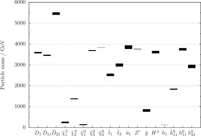
Refer to caption
Fig. 20: Dependence of the particle spectrum on the survival Higgs scale msurv=0.1subscript𝑚surv0.1m_{\text{surv}}=0.110 TeVtimes10teraelectronvolt10\text{\,}\mathrm{TeV} for parameter point PP1.

5.5 Benchmarks in the literature

As a final application of the threshold corrections presented here we now study the impact they have on previously published benchmarks in the model which have appeared in [8, 9, 10]. The 1 TeVtimes1teraelectronvolt1\text{\,}\mathrm{TeV} limit for the gluino which we require to be consistent with Atlas and CMS searches is above the masses of the all light benchmarks [8, 9], while heavy benchmarks [10] were chosen to be safe from these limits. However since the threshold effects presented here have a very large impact on the gluino mass, clearly they play an important role in determining whether or not a particular CE6SSM point is excluded. We will therefore study what impact the threshold effects have on all these points and in particular whether it changes their experimental status.121212All but one of the light benchmarks have a Zsuperscript𝑍Z^{\prime} mass substantially below the limit discussed in Sec. 5.3.2. Light exotics, like singlinos, which are necessarily present in the E6SSM, will give a substantial reduction in the limit. This is probably not sufficient to evade the limits, but nonetheless testing against constraints from gluino searches provides another important limitation on the viability of these scenarios.

The benchmarks in Refs. [8, 9] were selected to have very light gauginos or be close to the lower limit on m0subscript𝑚0m_{0} (for that choice of singlet VEV s𝑠s), where one can get lighter exotic sfermions. Below this lower limit on m0subscript𝑚0m_{0} the inert Higgs scalars become tachyonic due to the large U(1)N𝑈subscript1𝑁U(1)_{N} D𝐷D-terms which give a negative contribution to the mass.

As a result of this the threshold corrections can push some points into the region with tachyonic masses. Since we are applying the threshold corrections iteratively this creates a problem. It may be that such points in fact do not contain tachyonic solutions but merely the first step in the iteration jumps to that region and subsequent steps, if they could be performed, would lead to a self consistent tachyon free solution. In this case we try pushing the point into a convergent iteration by adjusting the thresholds corrections in the early steps. If this does not work we then vary the survival Higgs mass to see if this can lead to tachyon free solutions.

The impact on the gluino mass of these threshold corrections, for all the points is shown in Tab. 4 for μ=mH=mbarH=10 TeVsuperscript𝜇subscript𝑚superscript𝐻subscript𝑚barsuperscript𝐻times10teraelectronvolt\mu^{\prime}=m_{H^{\prime}}=m_{\mathrm{bar}{H}^{\prime}}=$10\text{\,}\mathrm{TeV}$, unless marked with a or b where the survival Higgs masses were varied until a self consistent solution could be found.

mg~subscript𝑚~𝑔m_{\tilde{g}} / GeV BMA BMB BMC BMD BME
without thresholds 336336336 330330330 353353353 327327327 338338338
including thresholds 224224224 269bsuperscript269𝑏269^{b} 260260260 230230230 203bsuperscript203𝑏203^{b}
mg~subscript𝑚~𝑔m_{\tilde{g}} / GeV BM1 BM2 BM3 BM4 BM5 BM6
without thresholds 350350350 673673673 362362362 642642642 338338338 805805805
including thresholds 322322322 613asuperscript613𝑎613^{a} 275275275 423asuperscript423𝑎423^{a} 190190190 825825825
mg~subscript𝑚~𝑔m_{\tilde{g}} / GeV HBM1 HBM2 HBM3 HBM4 HBM5
without thresholds 984984984 135213521352 165916591659 112911291129 100110011001
including thresholds 109010901090 149414941494 188618861886 827827827 106710671067
Tab. 4: Comparison of the originally reported gluino mass and the gluino mass including threshold corrections for previously published E6SSM benchmarks, where we have chosen μ=mH=mbarH=10 TeVsuperscript𝜇subscript𝑚superscript𝐻subscript𝑚barsuperscript𝐻times10teraelectronvolt\mu^{\prime}=m_{H^{\prime}}=m_{\mathrm{bar}{H}^{\prime}}=$10\text{\,}\mathrm{TeV}$ for all points except those marked a where we used μ=mH=mbarH=100 TeVsuperscript𝜇subscript𝑚superscript𝐻subscript𝑚barsuperscript𝐻times100teraelectronvolt\mu^{\prime}=m_{H^{\prime}}=m_{\mathrm{bar}{H}^{\prime}}=$100\text{\,}\mathrm{TeV}$ to evade tachyonic problems with convergence and b where they were increased to 104 TeVtimessuperscript104teraelectronvolt10^{4}\text{\,}\mathrm{TeV}.

But while the survival Higgs masses can have important effects, all light benchmarks are left with a gluino mass substantially below the limit. Therefore we can confirm that all of these points have been excluded by the LHC even when threshold effects are taken account of and the survival Higgs masses are varied without regard to maintaining gauge coupling unification.

The situation is more optimistic for the new heavy benchmarks proposed in [10]. These benchmarks were chosen to satisfy the latest LHC limits and also have the right relic density. For the benchmarks HBM1–HBM3 there are significant changes to the gluino mass as shown in the third column of Tab. 4 pushing them further away from current constraints. However beyond this all qualitative features remain unchanged with the Higgs mass staying in the Higgs signal range, though it is modified to 125 GeVtimes125gigaelectronvolt125\text{\,}\mathrm{GeV} for HBM1 and HBM3. The light inert Higgsinos, fixed to be light to achieve the correct relic abundance density, remain light and can be tuned carefully to match the relic abundance density measurement exactly without perturbing the rest of the spectrum. HBM2 and HBM3 also have light exotic quarks and these also stay light, with their masses reduced by approximately 4 %times4percent4\text{\,}\% and 6 %times6percent6\text{\,}\% respectively. Therefore the essential features of these benchmarks are not changed by the inclusion of threshold effects.

However for HBM4 and HBM5 the situation is more dramatic. These points have a very large singlet VEV, 50 TeVtimes50teraelectronvolt50\text{\,}\mathrm{TeV} and 100 TeVtimes100teraelectronvolt100\text{\,}\mathrm{TeV} respectively and in such cases while light gauginos can always be obtained, this is only achievable for a very narrow range of the input exotic Yukawa couplings. Consequentially when one varies these Yukawa couplings the masses can change a lot and the modification in these values (at low energies) from threshold corrections can result in very large changes to the soft masses. For HBM4 although a gluino mass of the same order is maintained the sign of M1/2subscript𝑀12M_{1/2} is actually changed, while for HBM5 a positive M1/2subscript𝑀12M_{1/2} is obtained but the stability of the result is not clear as scale variations lead to huge changes in the mass.

However these large changes in the physical spectrum are really an artifact of the choices for input/output parameters. One can instead try to match the values of m0subscript𝑚0m_{0}, M1/2subscript𝑀12M_{1/2} and then observe changes in the exotic Yukawa couplings. This would typically lead to a similar spectrum, though λ3subscript𝜆3\lambda_{3} affects the light Higgs mass and therefore the light Higgs mass is shifted.

6 Summary and conclusions

In this paper we have improved the prediction of low-scale quantities from high-scale parameters in the Exceptional Supersymmetric Standard Model (E6SSM). Full sparticle threshold corrections to the gauge couplings have been calculated by matching the E6SSM to the SM. Similarly, the low-scale DR¯¯DR\overline{\text{DR}} E6SSM Yukawa couplings have been calculated at the loop level directly from mass measurements of the SM fermions and mWsubscript𝑚𝑊m_{W}. Full expressions for these corrections are provided, and we have implemented them into an improved spectrum generator for the constrained E6SSM.

Using the spectrum generator, we have studied the impact of these corrections in detail. Both for the test point PP1 and in a parameter scan we found a dramatic reduction in the scale dependency of many masses, in particular of the gluino mass which is important for setting limits on the model from collider constraints. Also charginos, neutralinos, squarks and exotics receive large corrections. Even the smaller threshold effects for the light Higgs boson mass have a big impact on the allowed regions of parameter space due to our knowledge of the allowed values of the light Higgs mass, given recent LHC results on Higgs searches and the discovery of a new particle.

The new spectrum generator with the implemented corrections allows us to draw firmer conclusions about the allowed parameter space of the model. In line with previous results, we found a substantial region of parameter space where the mass of lightest Higgs is compatible with the new boson discovered at the LHC and the limits from collider searches for squark, gluinos and Zsuperscript𝑍Z^{\prime} bosons, are all satisfied. However the threshold corrections imply a significant change in the high-scale parameters where this is achieved and can alter the way these constraints combine.

An interesting consequence of the threshold corrections is a dependency of the mass spectrum on the survival Higgs fields, which are included in the model to assist gauge coupling unification. In previous studies these states simply decoupled from the rest of the spectrum. With the full sparticle threshold corrections included, we found that in most of the spectrum the dependency of the spectrum is rather weak. However if the dependence on the unknown survival Higgs masses is viewed as a theoretical uncertainty, this uncertainty is larger than that from the remaining scale variation, though much smaller than the uncertainty of earlier studies neglecting threshold corrections.

If the survival Higgs bosons are taken seriously as physical fields, the threshold corrections allow to fix their masses by the requirement of gauge coupling unification. Indeed we found that the survival Higgs masses can always be chosen such that gauge coupling unification is valid, up to hypothetical GUT threshold corrections, with required survival Higgs masses in the multi-TeV region.

Finally we looked at how the threshold corrections affect benchmark points that have previously appeared in the literature. Many benchmarks proposed in earlier papers appeared to be ruled out by gluino searches. We confirmed all of these to be ruled out once the threshold corrections are included. The benchmarks proposed more recently to be consistent with experiment receive significant corrections. Nonetheless these benchmarks are still experimentally viable after including the threshold corrections. For two benchmarks, HBM4 and HBM5, the stability of the predictions is poor due to fine tuning of input parameters required to get the very hierarchical spectrum these benchmarks illustrate.

In conclusion, our study shows that it is possible and valuable to take into account higher-order corrections to the high-scale–low-scale connection even in complicated, non-minimal supersymmetric models such as the E6SSM. The qualitative features of the CE6SSM itself have not been changed by the threshold corrections. Still, the model is theoretically attractive, predictive and viable. As more LHC data comes in, distinguishing between different supersymmetric models and hypotheses of GUT-scale physics becomes more relevant, and precise spectrum generators like the one presented here will be helpful.

Acknowledgements

The work of PA is supported by the ARC Centre of Excellence for Particle Physics at the Terascale, the work of AV is funded by the DFG Graduate College 1504, and we acknowledge financial support by the German Ministry for Science and Education. PA would like to thank S. F. King, A. Merle, D. J. Miller, M. Schönherr and Patrik Svantesson for helpful comments and discussions regarding this work.

Appendix A E6SSM covariant derivative and GUT relations

The E6subscript𝐸6E_{6} covariant derivative reads

Dμ=μ+ig0A~μbaraT~bara(bara=1,,78),subscript𝐷𝜇subscript𝜇isubscript𝑔0superscriptsubscript~𝐴𝜇bar𝑎superscript~𝑇bar𝑎bar𝑎178\displaystyle D_{\mu}=\partial_{\mu}+\mathrm{i}g_{0}\tilde{A}_{\mu}^{\mathrm{bar}{a}}\tilde{T}^{\mathrm{bar}{a}}\qquad\qquad(\mathrm{bar}{a}=1,\dotsc,78), (A.1)

with a single gauge coupling g0subscript𝑔0g_{0}, where T~barasuperscript~𝑇bar𝑎\tilde{T}^{\mathrm{bar}{a}} are the generators and A~μbarasuperscriptsubscript~𝐴𝜇bar𝑎\tilde{A}_{\mu}^{\mathrm{bar}{a}} are gauge fields in the adjoint representation (𝟕𝟖)78(\mathbf{78}) of the E6subscript𝐸6E_{6}. This covariant derivative can be decomposed in terms of the SU(3)c𝑆𝑈subscript3cSU(3)_{\text{c}}, SU(2)L𝑆𝑈subscript2LSU(2)_{\text{L}}, U(1)Y𝑈subscript1𝑌U(1)_{Y} and U(1)N𝑈subscript1𝑁U(1)_{N} sub-groups

Dμ=μ+ig3TaGμa+ig2τ2Wμ+igYY2Bμ+igNN2Zμ+subscript𝐷𝜇subscript𝜇isubscript𝑔3superscript𝑇𝑎superscriptsubscript𝐺𝜇𝑎isubscript𝑔2𝜏2subscript𝑊𝜇isubscript𝑔𝑌𝑌2subscript𝐵𝜇isubscript𝑔𝑁𝑁2subscriptsuperscript𝑍𝜇\displaystyle D_{\mu}=\partial_{\mu}+\mathrm{i}g_{3}T^{a}G_{\mu}^{a}+\mathrm{i}g_{2}\frac{\vec{\tau}}{2}\cdot\vec{W}_{\mu}+\mathrm{i}g_{Y}\frac{Y}{2}B_{\mu}+\mathrm{i}g_{N}\frac{N}{2}Z^{\prime}_{\mu}+\dotsb (A.2)

All generators in (A.2) are normalized such that the quantum numbers are the same as in Tab. 1. This, together with the condition TrTa~Ta~=δab/2Tr~superscript𝑇𝑎~superscript𝑇𝑎superscript𝛿𝑎𝑏2\operatorname{Tr}\tilde{T^{a}}\tilde{T^{a}}=\delta^{ab}/2, yields a GUT relation between the couplings

g3=g2=g1=g1=:g0,\displaystyle g_{3}=g_{2}=g_{1}=g_{1}^{\prime}=:g_{0}, (A.3)

where

g1subscript𝑔1\displaystyle g_{1} :=53gY,assignabsent53subscript𝑔𝑌\displaystyle:=\sqrt{\frac{5}{3}}\;g_{Y}, g1superscriptsubscript𝑔1\displaystyle g_{1}^{\prime} :=40gN.assignabsent40subscript𝑔𝑁\displaystyle:=\sqrt{40}\;g_{N}. (A.4)

At the electroweak scale the generator Q𝑄Q of the unbroken U(1)em𝑈subscript1emU(1)_{\text{em}} is then given by

Q=τ32+Y2.𝑄subscript𝜏32𝑌2\displaystyle Q=\frac{\tau_{3}}{2}+\frac{Y}{2}. (A.5)

Appendix B E6SSM mass eigenstates

B.1 Higgs sector

We write the Higgs bosons in the E6SSM as

Hpi=(Hpi1Hpi2),Si,subscript𝐻𝑝𝑖matrixsuperscriptsubscript𝐻𝑝𝑖1superscriptsubscript𝐻𝑝𝑖2subscript𝑆𝑖\displaystyle H_{pi}=\begin{pmatrix}H_{pi}^{1}\\ H_{pi}^{2}\end{pmatrix},\qquad S_{i}, (B.1)

where i=1,2,3𝑖123i=1,2,3 is the generation index and p=1,2𝑝12p=1,2 denotes the down (p=1𝑝1p=1) and up (p=2𝑝2p=2) Higgs bosons. When the SU(2)L×U(1)Y×U(1)N𝑆𝑈subscript2𝐿𝑈subscript1𝑌𝑈subscript1𝑁SU(2)_{L}\times U(1)_{Y}\times U(1)_{N} is broken to U(1)em.𝑈subscript1em.U(1)_{\text{em.}} the third generation Higgs bosons get a vacuum expectation value

H13subscript𝐻13\displaystyle H_{13} =(H130H13)(v12+eH130+imH130H13),absentmatrixsuperscriptsubscript𝐻130superscriptsubscript𝐻13matrixsubscript𝑣12esuperscriptsubscript𝐻130𝑖msuperscriptsubscript𝐻130superscriptsubscript𝐻13\displaystyle=\begin{pmatrix}H_{13}^{0}\\ H_{13}^{-}\end{pmatrix}\rightarrow\begin{pmatrix}\frac{v_{1}}{\sqrt{2}}+\operatorname{\Re e}H_{13}^{0}+i\operatorname{\Im m}H_{13}^{0}\\ H_{13}^{-}\end{pmatrix}, (B.2)
H23subscript𝐻23\displaystyle H_{23} =(H23+H230)(H23+v22+eH230+imH230),absentmatrixsuperscriptsubscript𝐻23superscriptsubscript𝐻230matrixsuperscriptsubscript𝐻23subscript𝑣22esuperscriptsubscript𝐻230𝑖msuperscriptsubscript𝐻230\displaystyle=\begin{pmatrix}H_{23}^{+}\\ H_{23}^{0}\end{pmatrix}\rightarrow\begin{pmatrix}H_{23}^{+}\\ \frac{v_{2}}{\sqrt{2}}+\operatorname{\Re e}H_{23}^{0}+i\operatorname{\Im m}H_{23}^{0}\end{pmatrix}, (B.3)
S3subscript𝑆3\displaystyle S_{3} s2+eS3+imS3.absent𝑠2esubscript𝑆3𝑖msubscript𝑆3\displaystyle\rightarrow\frac{s}{\sqrt{2}}+\operatorname{\Re e}S_{3}+i\operatorname{\Im m}S_{3}. (B.4)

Furthermore we define

tanβ:=v2v1,tanϕ:=v2ssin2β,μeff,i:=λis2.formulae-sequenceassign𝛽subscript𝑣2subscript𝑣1formulae-sequenceassignitalic-ϕ𝑣2𝑠2𝛽assignsubscript𝜇eff𝑖subscript𝜆𝑖𝑠2\displaystyle\tan\beta:=\frac{v_{2}}{v_{1}},\qquad\tan\phi:=\frac{v}{2s}\sin 2\beta,\qquad\mu_{\text{eff},i}:=\frac{\lambda_{i}s}{\sqrt{2}}. (B.5)

From the real parts of H130subscriptsuperscript𝐻013H^{0}_{13}, H230subscriptsuperscript𝐻023H^{0}_{23} and S3subscript𝑆3S_{3} we construct three CP even Higgs bosons. The diagonalization of the CP even mass matrix is done in two steps. At first we transform eH130esubscriptsuperscript𝐻013\operatorname{\Re e}H^{0}_{13}, eH230esubscriptsuperscript𝐻023\operatorname{\Re e}H^{0}_{23} and eS3esubscript𝑆3\operatorname{\Re e}S_{3} into intermediate states (𝗁1,𝗁2,𝗁3)subscript𝗁1subscript𝗁2subscript𝗁3(\mathsf{h}_{1},\mathsf{h}_{2},\mathsf{h}_{3}) via

(eH130eH230eS3)=UMSSM12(𝗁1𝗁2𝗁3)+12(v1v2s),matrixesubscriptsuperscript𝐻013esubscriptsuperscript𝐻023esubscript𝑆3subscript𝑈MSSM12matrixsubscript𝗁1subscript𝗁2subscript𝗁312matrixsubscript𝑣1subscript𝑣2𝑠\displaystyle\begin{pmatrix}\operatorname{\Re e}H^{0}_{13}\\ \operatorname{\Re e}H^{0}_{23}\\ \operatorname{\Re e}S_{3}\end{pmatrix}=U_{\text{MSSM}}\frac{1}{\sqrt{2}}\begin{pmatrix}\mathsf{h}_{1}\\ \mathsf{h}_{2}\\ \mathsf{h}_{3}\end{pmatrix}+\frac{1}{\sqrt{2}}\begin{pmatrix}v_{1}\\ v_{2}\\ s\end{pmatrix}, (B.6)

where the mixing matrix UMSSMsubscript𝑈MSSMU_{\text{MSSM}} has the form

UMSSM=(cosβsinβ0sinβcosβ0001).subscript𝑈MSSMmatrix𝛽𝛽0𝛽𝛽0001\displaystyle U_{\text{MSSM}}=\begin{pmatrix}\cos\beta&-\sin\beta&0\\ \sin\beta&\cos\beta&0\\ 0&0&1\end{pmatrix}. (B.7)

In the basis of 𝗁=(𝗁1,𝗁2,𝗁3)T𝗁superscriptsubscript𝗁1subscript𝗁2subscript𝗁3𝑇\mathsf{h}=(\mathsf{h}_{1},\mathsf{h}_{2},\mathsf{h}_{3})^{T} the Lagrangian for the CP even Higgs masses reads

even=12𝗁TMMSSM𝗁,subscripteven12superscript𝗁𝑇subscript𝑀MSSM𝗁\displaystyle\mathcal{L}_{\text{even}}=-\frac{1}{2}\mathsf{h}^{T}M_{\text{MSSM}}\mathsf{h}, (B.8)

where the matrix MMSSMsubscript𝑀MSSMM_{\text{MSSM}} is non-diagonal in general. Note, that the above transformation is analogous to the MSSM, where the mixing angle in UMSSMsubscript𝑈MSSMU_{\text{MSSM}} is β𝛽\beta. In a second step we diagonalize the mass matrix MMSSMsubscript𝑀MSSMM_{\text{MSSM}} by the unitary matrix UE6subscript𝑈subscript𝐸6U_{E_{6}}. The resulting CP even Higgs mass eigenstates are labeled h=(h1,h2,h3)Tsuperscriptsubscript1subscript2subscript3𝑇h=(h_{1},h_{2},h_{3})^{T}. The diagonalization transformation reads

h\displaystyle h =UE6𝗁,absentsubscript𝑈subscript𝐸6𝗁\displaystyle=U_{E_{6}}\mathsf{h}, ME6subscript𝑀subscript𝐸6\displaystyle M_{E_{6}} =UE6MMSSMUE6,absentsuperscriptsubscript𝑈subscript𝐸6subscript𝑀MSSMsuperscriptsubscript𝑈subscript𝐸6\displaystyle=U_{E_{6}}^{*}M_{\text{MSSM}}U_{E_{6}}^{\dagger}, (B.9)

where ME6subscript𝑀subscript𝐸6M_{E_{6}} is diagonal. From the gauge eigenstates 𝖠=(mH130,mH230,mS3)T𝖠superscriptmsubscriptsuperscript𝐻013msubscriptsuperscript𝐻023msubscript𝑆3𝑇\mathsf{A}=(\operatorname{\Im m}H^{0}_{13},\operatorname{\Im m}H^{0}_{23},\operatorname{\Im m}S_{3})^{T} we construct three CP odd Higgs boson mass eigenstates A=(A1,A2,A3)T(G0,G,A0)T𝐴superscriptsubscript𝐴1subscript𝐴2subscript𝐴3𝑇superscriptsuperscript𝐺0superscript𝐺superscript𝐴0𝑇A=(A_{1},A_{2},A_{3})^{T}\equiv(G^{0},G^{\prime},A^{0})^{T} via

12A12𝐴\displaystyle\frac{1}{\sqrt{2}}A :=UA𝖠,assignabsentsubscript𝑈𝐴𝖠\displaystyle:=U_{A}\mathsf{A}, MAsubscript𝑀𝐴\displaystyle M_{A} =UAMUA,absentsuperscriptsubscript𝑈𝐴𝑀superscriptsubscript𝑈𝐴\displaystyle=U_{A}^{*}MU_{A}^{\dagger}, (B.10)

where MAsubscript𝑀𝐴M_{A} is diagonal. The mixing matrix UAsubscript𝑈𝐴U_{A} is parametrized as

UA=(cosβsinβ0sinβsinϕcosβsinϕcosϕsinβcosϕcosβcosϕsinϕ).subscript𝑈𝐴matrix𝛽𝛽0𝛽italic-ϕ𝛽italic-ϕitalic-ϕ𝛽italic-ϕ𝛽italic-ϕitalic-ϕ\displaystyle U_{A}=\begin{pmatrix}\cos\beta&-\sin\beta&0\\ -\sin\beta\sin\phi&-\cos\beta\sin\phi&\cos\phi\\ \sin\beta\cos\phi&\cos\beta\cos\phi&\sin\phi\end{pmatrix}. (B.11)

The charged Higgs and goldstone bosons (Hi±)=(G±H±)Tsubscriptsuperscript𝐻plus-or-minus𝑖superscriptsuperscript𝐺plus-or-minussuperscript𝐻plus-or-minus𝑇(H^{\pm}_{i})=(G^{\pm}~{}H^{\pm})^{T} are constructed from the gauge eigenstates Hi3±superscriptsubscript𝐻𝑖3plus-or-minusH_{i3}^{\pm} via

Hi±subscriptsuperscript𝐻plus-or-minus𝑖\displaystyle H^{\pm}_{i} =Uij±Hj3±(i,j=1,2),\displaystyle=U^{\pm}_{ij}H^{\pm}_{j3}\quad(i,j=1,2), where U±superscript𝑈plus-or-minus\displaystyle U^{\pm} =(cosβsinβsinβcosβ).absentmatrix𝛽𝛽𝛽𝛽\displaystyle=\begin{pmatrix}\cos\beta&-\sin\beta\\ \sin\beta&\cos\beta\end{pmatrix}. (B.12)

B.2 Inert Higgs sector

The first two generations (i=1,2;p=1,2)formulae-sequence𝑖12𝑝12(i=1,2;~{}p=1,2) Higgs doublets in Eq. (B.1) are called inert Higgs bosons. For each generation i=1,2𝑖12i=1,2 we mix the fields H1i0superscriptsubscript𝐻1𝑖0H_{1i}^{0}, H2i0superscriptsubscript𝐻2𝑖0H_{2i}^{0*} to mass eigenstates hik0superscriptsubscript𝑖𝑘0h_{ik}^{0} with an unitary matrix Uinert0isuperscriptsubscript𝑈inert0𝑖U_{\text{inert}}^{0i} via

hik0=(Uinert0i)kl(H1i0H2i0)l,Uinert0i=(cosθi0sinθi0sinθi0cosθi0).formulae-sequencesuperscriptsubscript𝑖𝑘0subscriptsuperscriptsubscript𝑈inert0𝑖𝑘𝑙subscriptmatrixsuperscriptsubscript𝐻1𝑖0superscriptsubscript𝐻2𝑖0𝑙superscriptsubscript𝑈inert0𝑖matrixsuperscriptsubscript𝜃𝑖0superscriptsubscript𝜃𝑖0superscriptsubscript𝜃𝑖0superscriptsubscript𝜃𝑖0\displaystyle h_{ik}^{0}=(U_{\text{inert}}^{0i})_{kl}\begin{pmatrix}H_{1i}^{0}\\ H_{2i}^{0*}\end{pmatrix}_{l},\qquad U_{\text{inert}}^{0i}=\begin{pmatrix}\cos\theta_{i}^{0}&\sin\theta_{i}^{0}\\ -\sin\theta_{i}^{0}&\cos\theta_{i}^{0}\end{pmatrix}. (B.13)

Here k,l=1,2formulae-sequence𝑘𝑙12k,l=1,2 enumerates the mass eigenstates and we neglect inter-generation mixing. Furthermore for each generation i=1,2𝑖12i=1,2 we mix the fields H1isuperscriptsubscript𝐻1𝑖H_{1i}^{-}, H2i+superscriptsubscript𝐻2𝑖absentH_{2i}^{+*} to mass eigenstates hiksuperscriptsubscript𝑖𝑘h_{ik}^{-} with an unitary matrix Uinert±isuperscriptsubscript𝑈inertplus-or-minus𝑖U_{\text{inert}}^{\pm i} via

hik=(Uinert±i)kl(H1iH2i+)l,Uinert±i=(cosθi±sinθi±sinθi±cosθi±).formulae-sequencesuperscriptsubscript𝑖𝑘subscriptsuperscriptsubscript𝑈inertplus-or-minus𝑖𝑘𝑙subscriptmatrixsuperscriptsubscript𝐻1𝑖superscriptsubscript𝐻2𝑖absent𝑙superscriptsubscript𝑈inertplus-or-minus𝑖matrixsuperscriptsubscript𝜃𝑖plus-or-minussuperscriptsubscript𝜃𝑖plus-or-minussuperscriptsubscript𝜃𝑖plus-or-minussuperscriptsubscript𝜃𝑖plus-or-minus\displaystyle h_{ik}^{-}=(U_{\text{inert}}^{\pm i})_{kl}\begin{pmatrix}H_{1i}^{-}\\ H_{2i}^{+*}\end{pmatrix}_{l},\qquad U_{\text{inert}}^{\pm i}=\begin{pmatrix}\cos\theta_{i}^{\pm}&\sin\theta_{i}^{\pm}\\ -\sin\theta_{i}^{\pm}&\cos\theta_{i}^{\pm}\end{pmatrix}. (B.14)

Here k,l=1,2formulae-sequence𝑘𝑙12k,l=1,2 enumerates the mass eigenstates and we neglect inter-generation mixing. Furthermore for each generation i=1,2𝑖12i=1,2 we mix the fields H~1iL0superscriptsubscript~𝐻1𝑖𝐿0\tilde{H}_{1iL}^{0}, H~2iL0superscriptsubscript~𝐻2𝑖𝐿0\tilde{H}_{2iL}^{0} to mass eigenstates ψli0superscriptsubscript𝜓𝑙𝑖0\psi_{li}^{0} with an unitary matrix Z𝑍Z via

ψli0=Zln(H~1iL0H~2iL0)n,Z=12(1111).formulae-sequencesuperscriptsubscript𝜓𝑙𝑖0subscript𝑍𝑙𝑛subscriptmatrixsuperscriptsubscript~𝐻1𝑖𝐿0superscriptsubscript~𝐻2𝑖𝐿0𝑛𝑍12matrix1111\displaystyle\psi_{li}^{0}=Z_{ln}\begin{pmatrix}\tilde{H}_{1iL}^{0}\\ \tilde{H}_{2iL}^{0}\end{pmatrix}_{n},\qquad Z=\frac{1}{\sqrt{2}}\begin{pmatrix}1&1\\ -1&1\end{pmatrix}. (B.15)

The Majorana mass eigenstates are then defined as

h~li0=(ψli0ψli0¯T).superscriptsubscript~𝑙𝑖0matrixsuperscriptsubscript𝜓𝑙𝑖0superscript¯superscriptsubscript𝜓𝑙𝑖0𝑇\displaystyle\tilde{h}_{li}^{0}=\begin{pmatrix}\psi_{li}^{0}\\ \overline{\psi_{li}^{0}}^{T}\end{pmatrix}. (B.16)

For each generation i=1,2𝑖12i=1,2 we combine the fields H~1iLsuperscriptsubscript~𝐻1𝑖𝐿\tilde{H}_{1iL}^{-}, H~2iL+¯Tsuperscript¯superscriptsubscript~𝐻2𝑖𝐿𝑇\overline{\tilde{H}_{2iL}^{+}}^{T} to mass eigenstates h~isuperscriptsubscript~𝑖\tilde{h}_{i}^{-} via

h~i=(H~1iLH~2iL+¯T).superscriptsubscript~𝑖matrixsuperscriptsubscript~𝐻1𝑖𝐿superscript¯superscriptsubscript~𝐻2𝑖𝐿𝑇\displaystyle\tilde{h}_{i}^{-}=\begin{pmatrix}\tilde{H}_{1iL}^{-}\\ \overline{\tilde{H}_{2iL}^{+}}^{T}\end{pmatrix}. (B.17)

B.3 Survival Higgs sector

We mix the neutral survival Higgs bosons H0superscriptsuperscript𝐻0{H^{\prime}}^{0}, barH0barsuperscriptsuperscript𝐻0\mathrm{bar}{H^{\prime}}^{0*} to mass eigenstates hk0superscriptsubscriptsuperscript𝑘0{h^{\prime}}_{k}^{0} with an unitary matrix Usurv0superscriptsubscript𝑈surv0U_{\text{surv}}^{0} via

hk0=(Usurv0)kl(H0barH0)l,Usurv0=(cosθ0sinθ0sinθ0cosθ0).formulae-sequencesuperscriptsubscriptsuperscript𝑘0subscriptsuperscriptsubscript𝑈surv0𝑘𝑙subscriptmatrixsuperscriptsuperscript𝐻0barsuperscriptsuperscript𝐻0𝑙superscriptsubscript𝑈surv0matrixsuperscript𝜃0superscript𝜃0superscript𝜃0superscript𝜃0\displaystyle{h^{\prime}}_{k}^{0}=(U_{\text{surv}}^{0})_{kl}\begin{pmatrix}{H^{\prime}}^{0}\\ \mathrm{bar}{H^{\prime}}^{0*}\end{pmatrix}_{l},\qquad U_{\text{surv}}^{0}=\begin{pmatrix}\cos\theta^{\prime 0}&\sin\theta^{\prime 0}\\ -\sin\theta^{\prime 0}&\cos\theta^{\prime 0}\end{pmatrix}. (B.18)

We mix the charged survival Higgs bosons Hsuperscriptsuperscript𝐻{H^{\prime}}^{-}, barH+barsuperscriptsuperscript𝐻absent\mathrm{bar}{H^{\prime}}^{+*} to mass eigenstates hksuperscriptsubscriptsuperscript𝑘{h^{\prime}}_{k}^{-} with an unitary matrix Usurv±superscriptsubscript𝑈survplus-or-minusU_{\text{surv}}^{\pm} via

hk=(Usurv±)kl(HbarH+)l,Usurv±=(cosθ±sinθ±sinθ±cosθ±).formulae-sequencesuperscriptsubscriptsuperscript𝑘subscriptsuperscriptsubscript𝑈survplus-or-minus𝑘𝑙subscriptmatrixsuperscriptsuperscript𝐻barsuperscriptsuperscript𝐻absent𝑙superscriptsubscript𝑈survplus-or-minusmatrixsuperscript𝜃plus-or-minussuperscript𝜃plus-or-minussuperscript𝜃plus-or-minussuperscript𝜃plus-or-minus\displaystyle{h^{\prime}}_{k}^{-}=(U_{\text{surv}}^{\pm})_{kl}\begin{pmatrix}{H^{\prime}}^{-}\\ \mathrm{bar}{H^{\prime}}^{+*}\end{pmatrix}_{l},\qquad U_{\text{surv}}^{\pm}=\begin{pmatrix}\cos\theta^{\prime\pm}&\sin\theta^{\prime\pm}\\ -\sin\theta^{\prime\pm}&\cos\theta^{\prime\pm}\end{pmatrix}. (B.19)

The survival higgsinos obey the same mixing as the neutral and charged inert higgsinos in Sec. B.2. We write the mass eigenstates as h~±superscript~plus-or-minus\tilde{h}^{\prime\pm} and h~i0superscriptsubscript~𝑖0\tilde{h}_{i}^{\prime 0} (i=1,2𝑖12i=1,2).

Appendix C E6SSM self-energies

C.1 W𝑊W boson

The W±superscript𝑊plus-or-minusW^{\pm} boson 1PI correlation function is decomposed into a transverse and longitudinal part as follows

ΓWμ+Wν(p)=gμν(p2mW2)(gμνpμpνp2)ΠWW,T(p2)pμpνp2ΠWW,L(p2),subscriptΓsuperscriptsubscript𝑊𝜇superscriptsubscript𝑊𝜈𝑝superscript𝑔𝜇𝜈superscript𝑝2superscriptsubscript𝑚𝑊2superscript𝑔𝜇𝜈superscript𝑝𝜇superscript𝑝𝜈superscript𝑝2subscriptΠ𝑊𝑊𝑇superscript𝑝2superscript𝑝𝜇superscript𝑝𝜈superscript𝑝2subscriptΠ𝑊𝑊𝐿superscript𝑝2\displaystyle\Gamma_{W_{\mu}^{+}W_{\nu}^{-}}(p)=-g^{\mu\nu}(p^{2}-m_{W}^{2})-\left(g^{\mu\nu}-\frac{p^{\mu}p^{\nu}}{p^{2}}\right)\Pi_{WW,T}(p^{2})-\frac{p^{\mu}p^{\nu}}{p^{2}}\Pi_{WW,L}(p^{2}), (C.1)

where the transverse part is in the E6SSM given by

(4π)2g22ΠWW,TE6SSM(p2)superscript4𝜋2superscriptsubscript𝑔22superscriptsubscriptΠ𝑊𝑊𝑇E6SSMsuperscript𝑝2\displaystyle\frac{(4\pi)^{2}}{g_{2}^{2}}\Pi_{WW,T}^{\text{E${}_{6}$SSM}}(p^{2}) =14i=13k=12{(UikA)2A0(mAi)+(UikE6)2A0(mhi)}absent14superscriptsubscript𝑖13superscriptsubscript𝑘12superscriptsuperscriptsubscript𝑈𝑖𝑘𝐴2subscript𝐴0subscript𝑚subscript𝐴𝑖superscriptsuperscriptsubscript𝑈𝑖𝑘subscript𝐸62subscript𝐴0subscript𝑚subscript𝑖\displaystyle=\frac{1}{4}\sum_{i=1}^{3}\sum_{k=1}^{2}\left\{\left(U_{ik}^{A*}\right)^{2}A_{0}(m_{A_{i}})+\left(U_{ik}^{E_{6}*}\right)^{2}A_{0}(m_{h_{i}})\right\}
+12A0(mH±)+12A0(mG±)+mW2i=13(Ui1E6)2B0(p2,mhi,mW)12subscript𝐴0subscript𝑚superscript𝐻plus-or-minus12subscript𝐴0subscript𝑚superscript𝐺plus-or-minussuperscriptsubscript𝑚𝑊2superscriptsubscript𝑖13superscriptsuperscriptsubscript𝑈𝑖1subscript𝐸62subscript𝐵0superscript𝑝2subscript𝑚subscript𝑖subscript𝑚𝑊\displaystyle\phantom{{}=}+\frac{1}{2}A_{0}(m_{H^{\pm}})+\frac{1}{2}A_{0}(m_{G^{\pm}})+m_{W}^{2}\sum_{i=1}^{3}\left(U_{i1}^{E_{6}*}\right)^{2}B_{0}(p^{2},m_{h_{i}},m_{W})
i=13j=12|Ui1AUj1±+Ui2AUj2±|2B22(p2,mAi,mHj±)superscriptsubscript𝑖13superscriptsubscript𝑗12superscriptsuperscriptsubscript𝑈𝑖1𝐴superscriptsubscript𝑈𝑗1plus-or-minussuperscriptsubscript𝑈𝑖2𝐴superscriptsubscript𝑈𝑗2plus-or-minus2subscript𝐵22superscript𝑝2subscript𝑚subscript𝐴𝑖subscript𝑚superscriptsubscript𝐻𝑗plus-or-minus\displaystyle\phantom{{}=}-\sum_{i=1}^{3}\sum_{j=1}^{2}\left|U_{i1}^{A}U_{j1}^{\pm}+U_{i2}^{A}U_{j2}^{\pm}\right|^{2}B_{22}(p^{2},m_{A_{i}},m_{H_{j}^{\pm}})
i=13j=12|k=13UikE6(U1kMSSMUj1±U2kMSSMUj2±)|2B22(p2,mAi,mHj±)superscriptsubscript𝑖13superscriptsubscript𝑗12superscriptsuperscriptsubscript𝑘13superscriptsubscript𝑈𝑖𝑘subscript𝐸6superscriptsubscript𝑈1𝑘MSSMsuperscriptsubscript𝑈𝑗1plus-or-minussuperscriptsubscript𝑈2𝑘MSSMsuperscriptsubscript𝑈𝑗2plus-or-minus2subscript𝐵22superscript𝑝2subscript𝑚subscript𝐴𝑖subscript𝑚superscriptsubscript𝐻𝑗plus-or-minus\displaystyle\phantom{{}=}-\sum_{i=1}^{3}\sum_{j=1}^{2}\left|\sum_{k=1}^{3}U_{ik}^{E_{6}}\left(U_{1k}^{\text{MSSM}}U_{j1}^{\pm}-U_{2k}^{\text{MSSM}}U_{j2}^{\pm}\right)\right|^{2}B_{22}(p^{2},m_{A_{i}},m_{H_{j}^{\pm}})
+i,l=12{12(|Zl1|2+|Zl2|2)H(p2,mh~i+,mh~li0)\displaystyle\phantom{{}=}+\sum_{i,l=1}^{2}\bigg{\{}\frac{1}{2}\left(|Z_{l1}|^{2}+|Z_{l2}|^{2}\right)H(p^{2},m_{{\tilde{h}}_{i}^{+}},m_{{\tilde{h}}_{li}^{0}})
2Zl1Zl2mh~i+mh~li0B0(p2,mh~i+,mh~li0)}\displaystyle\phantom{{}=\sum_{i,l=1}^{2}\bigg{\{}}-2Z_{l1}Z_{l2}m_{{\tilde{h}}_{i}^{+}}m_{{\tilde{h}}_{li}^{0}}B_{0}(p^{2},m_{{\tilde{h}}_{i}^{+}},m_{{\tilde{h}}_{li}^{0}})\bigg{\}}
2i=12{cos2(θi0+θi±)(B~22(p2,mhi1±,mhi10)+B~22(p2,mhi2±,mhi20))\displaystyle\phantom{{}=}-2\sum_{i=1}^{2}\Big{\{}\cos^{2}(\theta_{i}^{0}+\theta_{i}^{\pm})\left(\widetilde{B}_{22}(p^{2},m_{h_{i1}^{\pm}},m_{h_{i1}^{0}})+\widetilde{B}_{22}(p^{2},m_{h_{i2}^{\pm}},m_{h_{i2}^{0}})\right)
+sin2(θi0+θi±)(B~22(p2,mhi1±,mhi20)+B~22(p2,mhi2±,mhi10))}\displaystyle\phantom{{}=-2\sum_{i=1}^{2}\Big{\{}}+\sin^{2}(\theta_{i}^{0}+\theta_{i}^{\pm})\left(\widetilde{B}_{22}(p^{2},m_{h_{i1}^{\pm}},m_{h_{i2}^{0}})+\widetilde{B}_{22}(p^{2},m_{h_{i2}^{\pm}},m_{h_{i1}^{0}})\right)\Big{\}}
+l=12{12(|Zl1|2+|Zl2|2)H(p2,mh~+,mh~l0)\displaystyle\phantom{{}=}+\sum_{l=1}^{2}\bigg{\{}\frac{1}{2}\left(|Z^{\prime}_{l1}|^{2}+|Z^{\prime}_{l2}|^{2}\right)H(p^{2},m_{\tilde{h}^{\prime+}},m_{\tilde{h}_{l}^{\prime 0}})
2Zl1Zl2mh~+mh~l0B0(p2,mh~+,mh~l0)}\displaystyle\phantom{{}=\sum_{l=1}^{2}\bigg{\{}}-2Z^{\prime}_{l1}Z^{\prime}_{l2}m_{\tilde{h}^{\prime+}}m_{\tilde{h}_{l}^{\prime 0}}B_{0}(p^{2},m_{\tilde{h}^{\prime+}},m_{\tilde{h}_{l}^{\prime 0}})\bigg{\}}
2i=12{cos2(θ0+θ±)(B~22(p2,mh1±,mh10)+B~22(p2,mh2±,mh20))\displaystyle\phantom{{}=}-2\sum_{i=1}^{2}\Big{\{}\cos^{2}(\theta^{\prime 0}+\theta^{\prime\pm})\left(\widetilde{B}_{22}(p^{2},m_{{h^{\prime}}_{1}^{\pm}},m_{{h^{\prime}}_{1}^{0}})+\widetilde{B}_{22}(p^{2},m_{{h^{\prime}}_{2}^{\pm}},m_{{h^{\prime}}_{2}^{0}})\right)
+sin2(θ0+θ±)(B~22(p2,mh1±,mh20)+B~22(p2,mh2±,mh10))}\displaystyle\phantom{{}=-2\sum_{i=1}^{2}\Big{\{}}+\sin^{2}(\theta^{\prime 0}+\theta^{\prime\pm})\left(\widetilde{B}_{22}(p^{2},m_{{h^{\prime}}_{1}^{\pm}},m_{{h^{\prime}}_{2}^{0}})+\widetilde{B}_{22}(p^{2},m_{{h^{\prime}}_{2}^{\pm}},m_{{h^{\prime}}_{1}^{0}})\right)\Big{\}}
+4mW2gN2g22{(NH132+NH232)2sin2βcos2βB0(p2,mH±,mZ)\displaystyle\phantom{{}=}+4m_{W}^{2}\frac{g_{N}^{2}}{g_{2}^{2}}\bigg{\{}\left(\frac{N_{H_{13}}}{2}+\frac{N_{H_{23}}}{2}\right)^{2}\sin^{2}\beta\cos^{2}\beta B_{0}(p^{2},m_{H^{\pm}},m_{Z^{\prime}})
+(NH232sin2βNH132cos2β)2B0(p2,mG±,mZ)}\displaystyle\phantom{{}=4m_{W}^{2}\frac{g_{N}^{2}}{g_{2}^{2}}\bigg{\{}}+\left(\frac{N_{H_{23}}}{2}\sin^{2}\beta-\frac{N_{H_{13}}}{2}\cos^{2}\beta\right)^{2}B_{0}(p^{2},m_{G^{\pm}},m_{Z^{\prime}})\bigg{\}}
sW2(8B~22(p2,mW,0)+4p2B0(p2,mW,0))superscriptsubscript𝑠𝑊28subscript~𝐵22superscript𝑝2subscript𝑚𝑊04superscript𝑝2subscript𝐵0superscript𝑝2subscript𝑚𝑊0\displaystyle\phantom{{}=}-s_{W}^{2}\left(8\widetilde{B}_{22}(p^{2},m_{W},0)+4p^{2}B_{0}(p^{2},m_{W},0)\right)
{(4p2+mZ2+mW2)cW2mZ2sW4}B0(p2,mZ,mW)4superscript𝑝2superscriptsubscript𝑚𝑍2superscriptsubscript𝑚𝑊2superscriptsubscript𝑐𝑊2superscriptsubscript𝑚𝑍2superscriptsubscript𝑠𝑊4subscript𝐵0superscript𝑝2subscript𝑚𝑍subscript𝑚𝑊\displaystyle\phantom{{}=}-\left\{(4p^{2}+m_{Z}^{2}+m_{W}^{2})c_{W}^{2}-m_{Z}^{2}s_{W}^{4}\right\}B_{0}(p^{2},m_{Z},m_{W})
8cW2B~22(p2,mZ,mW)8superscriptsubscript𝑐𝑊2subscript~𝐵22superscript𝑝2subscript𝑚𝑍subscript𝑚𝑊\displaystyle\phantom{{}=}-8c_{W}^{2}\widetilde{B}_{22}(p^{2},m_{Z},m_{W})
+fu/fd{12NcfH(p2,mu,md)i,j=122Ncfwfij2B~22(p2,mu~i,md~j)}subscriptsubscript𝑓𝑢subscript𝑓𝑑12superscriptsubscript𝑁𝑐𝑓𝐻superscript𝑝2subscript𝑚𝑢subscript𝑚𝑑superscriptsubscript𝑖𝑗122superscriptsubscript𝑁𝑐𝑓superscriptsubscript𝑤𝑓𝑖𝑗2subscript~𝐵22superscript𝑝2subscript𝑚subscript~𝑢𝑖subscript𝑚subscript~𝑑𝑗\displaystyle\phantom{{}=}+\sum_{f_{u}/f_{d}}\left\{\frac{1}{2}N_{c}^{f}H(p^{2},m_{u},m_{d})-\sum_{i,j=1}^{2}2N_{c}^{f}w_{fij}^{2}\widetilde{B}_{22}(p^{2},m_{\tilde{u}_{i}},m_{\tilde{d}_{j}})\right\}
+1g22i=16j=12{fijWH(p2,mχ~i0,mχ~j+)+2gijWmχ~i0mχ~j+B0(p2,mχ~i0,mχ~j+)}1superscriptsubscript𝑔22superscriptsubscript𝑖16superscriptsubscript𝑗12subscript𝑓𝑖𝑗𝑊𝐻superscript𝑝2subscript𝑚subscriptsuperscript~𝜒0𝑖subscript𝑚subscriptsuperscript~𝜒𝑗2subscript𝑔𝑖𝑗𝑊subscript𝑚subscriptsuperscript~𝜒0𝑖subscript𝑚subscriptsuperscript~𝜒𝑗subscript𝐵0superscript𝑝2subscript𝑚subscriptsuperscript~𝜒0𝑖subscript𝑚subscriptsuperscript~𝜒𝑗\displaystyle\phantom{{}=}+\frac{1}{g_{2}^{2}}\sum_{i=1}^{6}\sum_{j=1}^{2}\bigg{\{}f_{ijW}H(p^{2},m_{\tilde{\chi}^{0}_{i}},m_{\tilde{\chi}^{+}_{j}})+2g_{ijW}m_{\tilde{\chi}^{0}_{i}}m_{\tilde{\chi}^{+}_{j}}B_{0}(p^{2},m_{\tilde{\chi}^{0}_{i}},m_{\tilde{\chi}^{+}_{j}})\bigg{\}} (C.2)

Analogous to [59] the summation fu/fdsubscriptsubscript𝑓𝑢subscript𝑓𝑑\sum_{f_{u}/f_{d}} is over quark and lepton doublets and

(wfij)=(cucdcusdsucdsusd).subscript𝑤𝑓𝑖𝑗matrixsubscript𝑐𝑢subscript𝑐𝑑subscript𝑐𝑢subscript𝑠𝑑subscript𝑠𝑢subscript𝑐𝑑subscript𝑠𝑢subscript𝑠𝑑\displaystyle(w_{fij})=\begin{pmatrix}c_{u}c_{d}&c_{u}s_{d}\\ s_{u}c_{d}&s_{u}s_{d}\end{pmatrix}. (C.3)

The neutralino–chargino–W-boson couplings are given by

fijWsubscript𝑓𝑖𝑗𝑊\displaystyle f_{ijW} =|aχ~i0χ~j+W|2+|bχ~i0χ~j+W|2,absentsuperscriptsubscript𝑎superscriptsubscript~𝜒𝑖0superscriptsubscript~𝜒𝑗𝑊2superscriptsubscript𝑏superscriptsubscript~𝜒𝑖0superscriptsubscript~𝜒𝑗𝑊2\displaystyle=|a_{\tilde{\chi}_{i}^{0}\tilde{\chi}_{j}^{+}W}|^{2}+|b_{\tilde{\chi}_{i}^{0}\tilde{\chi}_{j}^{+}W}|^{2}, gijWsubscript𝑔𝑖𝑗𝑊\displaystyle g_{ijW} =2e(bχ~i0χ~j+Waχ~i0χ~j+W),absent2esubscriptsuperscript𝑏superscriptsubscript~𝜒𝑖0superscriptsubscript~𝜒𝑗𝑊subscript𝑎superscriptsubscript~𝜒𝑖0superscriptsubscript~𝜒𝑗𝑊\displaystyle=2\operatorname{\Re e}\left(b^{*}_{\tilde{\chi}_{i}^{0}\tilde{\chi}_{j}^{+}W}a_{\tilde{\chi}_{i}^{0}\tilde{\chi}_{j}^{+}W}\right), (C.4)

where the Feynman rule for the neutralino–chargino–Wμsubscript𝑊𝜇W_{\mu} vertex is written as iγμ(a𝒫L+b𝒫R)𝑖subscript𝛾𝜇𝑎subscript𝒫𝐿𝑏subscript𝒫𝑅-i\gamma_{\mu}(a{\cal P}_{L}+b{\cal P}_{R}). The nonzero couplings in the E6SSM are the same as in the MSSM

aψ~20ψ~1+Wsubscript𝑎superscriptsubscript~𝜓20superscriptsubscript~𝜓1𝑊\displaystyle a_{\tilde{\psi}_{2}^{0}\tilde{\psi}_{1}^{+}W} =bψ~20ψ~1+W=g2,absentsubscript𝑏superscriptsubscript~𝜓20superscriptsubscript~𝜓1𝑊subscript𝑔2\displaystyle=b_{\tilde{\psi}_{2}^{0}\tilde{\psi}_{1}^{+}W}=-g_{2}, aψ~40ψ~2+Wsubscript𝑎superscriptsubscript~𝜓40superscriptsubscript~𝜓2𝑊\displaystyle a_{\tilde{\psi}_{4}^{0}\tilde{\psi}_{2}^{+}W} =bψ~30ψ~2+W=g22.absentsubscript𝑏superscriptsubscript~𝜓30superscriptsubscript~𝜓2𝑊subscript𝑔22\displaystyle=-b_{\tilde{\psi}_{3}^{0}\tilde{\psi}_{2}^{+}W}=\frac{g_{2}}{\sqrt{2}}. (C.5)

The couplings to mass eigenstates for an incoming neutralino χ~i0superscriptsubscript~𝜒𝑖0\tilde{\chi}_{i}^{0} are

aχ~i0χ~j+Wsubscript𝑎superscriptsubscript~𝜒𝑖0superscriptsubscript~𝜒𝑗𝑊\displaystyle a_{\tilde{\chi}_{i}^{0}\tilde{\chi}_{j}^{+}W} =NikVjlaψ~k0ψ~l+W,absentsuperscriptsubscript𝑁𝑖𝑘subscript𝑉𝑗𝑙subscript𝑎superscriptsubscript~𝜓𝑘0superscriptsubscript~𝜓𝑙𝑊\displaystyle=N_{ik}^{*}V_{jl}a_{\tilde{\psi}_{k}^{0}\tilde{\psi}_{l}^{+}W}, bχ~i0χ~j+Wsubscript𝑏superscriptsubscript~𝜒𝑖0superscriptsubscript~𝜒𝑗𝑊\displaystyle b_{\tilde{\chi}_{i}^{0}\tilde{\chi}_{j}^{+}W} =NikUjlbψ~k0ψ~l+W,absentsubscript𝑁𝑖𝑘superscriptsubscript𝑈𝑗𝑙subscript𝑏superscriptsubscript~𝜓𝑘0superscriptsubscript~𝜓𝑙𝑊\displaystyle=N_{ik}U_{jl}^{*}b_{\tilde{\psi}_{k}^{0}\tilde{\psi}_{l}^{+}W}, (C.6)

while for an incoming chargino χ~j+superscriptsubscript~𝜒𝑗\tilde{\chi}_{j}^{+} the couplings read

aχ~i0χ~j+Wsubscript𝑎superscriptsubscript~𝜒𝑖0superscriptsubscript~𝜒𝑗𝑊\displaystyle a_{\tilde{\chi}_{i}^{0}\tilde{\chi}_{j}^{+}W} =NikVjlaψ~k0ψ~l+W,absentsubscript𝑁𝑖𝑘superscriptsubscript𝑉𝑗𝑙subscript𝑎superscriptsubscript~𝜓𝑘0superscriptsubscript~𝜓𝑙𝑊\displaystyle=N_{ik}V_{jl}^{*}a_{\tilde{\psi}_{k}^{0}\tilde{\psi}_{l}^{+}W}, bχ~i0χ~j+Wsubscript𝑏superscriptsubscript~𝜒𝑖0superscriptsubscript~𝜒𝑗𝑊\displaystyle b_{\tilde{\chi}_{i}^{0}\tilde{\chi}_{j}^{+}W} =NikUjlbψ~k0ψ~l+W.absentsuperscriptsubscript𝑁𝑖𝑘subscript𝑈𝑗𝑙subscript𝑏superscriptsubscript~𝜓𝑘0superscriptsubscript~𝜓𝑙𝑊\displaystyle=N_{ik}^{*}U_{jl}b_{\tilde{\psi}_{k}^{0}\tilde{\psi}_{l}^{+}W}. (C.7)

C.2 Fermions

We decompose the fermion 1PI correlation function as

Γfbarf(p)=(PLΓfbarfL(p2)+PRΓfbarfR(p2))+PLΓfbarfl(p2)+PRΓfbarfr(p2)subscriptΓ𝑓bar𝑓𝑝italic-p̸subscript𝑃𝐿superscriptsubscriptΓ𝑓bar𝑓𝐿superscript𝑝2subscript𝑃𝑅superscriptsubscriptΓ𝑓bar𝑓𝑅superscript𝑝2subscript𝑃𝐿superscriptsubscriptΓ𝑓bar𝑓𝑙superscript𝑝2subscript𝑃𝑅superscriptsubscriptΓ𝑓bar𝑓𝑟superscript𝑝2\displaystyle\Gamma_{f\mathrm{bar}{f}}(p)=\not{p}\left(P_{L}\Gamma_{f\mathrm{bar}{f}}^{L}(p^{2})+P_{R}\Gamma_{f\mathrm{bar}{f}}^{R}(p^{2})\right)+P_{L}\Gamma_{f\mathrm{bar}{f}}^{l}(p^{2})+P_{R}\Gamma_{f\mathrm{bar}{f}}^{r}(p^{2}) (C.8)

and then define the fermion self-energy to be

Σf(p2):=12{mf[ΓfbarfL(p2)+ΓfbarfR(p2)]+Γfbarfl(p2)+Γfbarfr(p2)}.assignsubscriptΣ𝑓superscript𝑝212subscript𝑚𝑓delimited-[]superscriptsubscriptΓ𝑓bar𝑓𝐿superscript𝑝2superscriptsubscriptΓ𝑓bar𝑓𝑅superscript𝑝2superscriptsubscriptΓ𝑓bar𝑓𝑙superscript𝑝2superscriptsubscriptΓ𝑓bar𝑓𝑟superscript𝑝2\displaystyle\Sigma_{f}(p^{2}):=\frac{1}{2}\left\{m_{f}\left[\Gamma_{f\mathrm{bar}{f}}^{L}(p^{2})+\Gamma_{f\mathrm{bar}{f}}^{R}(p^{2})\right]+\Gamma_{f\mathrm{bar}{f}}^{l}(p^{2})+\Gamma_{f\mathrm{bar}{f}}^{r}(p^{2})\right\}. (C.9)

In the E6SSM it is given by

(4π)2Σt(p2)mtsuperscript4𝜋2subscriptΣ𝑡superscript𝑝2subscript𝑚𝑡\displaystyle(4\pi)^{2}\frac{\Sigma_{t}(p^{2})}{m_{t}} =4g323{B1(p2,mg~,mt~1)+B1(p2,mg~,mt~2)(5+3lnμ2mt2)\displaystyle=\frac{4g_{3}^{2}}{3}\Biggl{\{}B_{1}(p^{2},m_{\tilde{g}},m_{\tilde{t}_{1}})+B_{1}(p^{2},m_{\tilde{g}},m_{\tilde{t}_{2}})-\biggl{(}5+3\ln\frac{\mu^{2}}{m^{2}_{t}}\biggr{)}
sin(2θt)mg~mt(B0(p2,mg~,mt~1)B0(p2,mg~,mt~2))}\displaystyle\phantom{{}=}\qquad-\sin(2\theta_{t})\frac{m_{\tilde{g}}}{m_{t}}\left(B_{0}(p^{2},m_{\tilde{g}},m_{\tilde{t}_{1}})-B_{0}(p^{2},m_{\tilde{g}},m_{\tilde{t}_{2}})\right)\Biggr{\}}
+yt22i=13{A¯ti2[B1(p2,mt,mhi)+B0(p2,mt,mhi)]\displaystyle\phantom{{}=}+\frac{y_{t}^{2}}{2}\sum_{i=1}^{3}\bigg{\{}\underline{A}_{ti}^{2}\left[B_{1}(p^{2},m_{t},m_{h_{i}})+B_{0}(p^{2},m_{t},m_{h_{i}})\right]
+B¯ti2[B1(p2,mt,mAi)B0(p2,mt,mAi)]}\displaystyle\phantom{{}=}\phantom{+\frac{1}{2}y_{t}^{2}\sum_{i=1}^{3}\bigg{\{}}+\underline{B}_{ti}^{2}\left[B_{1}(p^{2},m_{t},m_{A_{i}})-B_{0}(p^{2},m_{t},m_{A_{i}})\right]\bigg{\}}
+12[(yb2sβ2+yt2cβ2)B1(p2,mb,mH+)+(g22+yb2cβ2+yt2sβ2)B1(p2,mb,mW)]12delimited-[]subscriptsuperscript𝑦2𝑏subscriptsuperscript𝑠2𝛽subscriptsuperscript𝑦2𝑡subscriptsuperscript𝑐2𝛽subscript𝐵1superscript𝑝2subscript𝑚𝑏subscript𝑚superscript𝐻superscriptsubscript𝑔22superscriptsubscript𝑦𝑏2superscriptsubscript𝑐𝛽2subscriptsuperscript𝑦2𝑡subscriptsuperscript𝑠2𝛽subscript𝐵1superscript𝑝2subscript𝑚𝑏subscript𝑚𝑊\displaystyle\phantom{{}=}+\frac{1}{2}\biggl{[}(y^{2}_{b}s^{2}_{\beta}+y^{2}_{t}c^{2}_{\beta})B_{1}(p^{2},m_{b},m_{H^{+}})+(g_{2}^{2}+y_{b}^{2}c_{\beta}^{2}+y^{2}_{t}s^{2}_{\beta})B_{1}(p^{2},m_{b},m_{W})\biggr{]}
+yb2cβ2[B0(p2,mb,mH+)B0(p2,mb,mW)](eet)2(5+3lnμ2mt2)superscriptsubscript𝑦𝑏2superscriptsubscript𝑐𝛽2delimited-[]subscript𝐵0superscript𝑝2subscript𝑚𝑏subscript𝑚superscript𝐻subscript𝐵0superscript𝑝2subscript𝑚𝑏subscript𝑚𝑊superscript𝑒subscript𝑒𝑡253superscript𝜇2subscriptsuperscript𝑚2𝑡\displaystyle\phantom{{}=}+y_{b}^{2}c_{\beta}^{2}\biggl{[}B_{0}(p^{2},m_{b},m_{H^{+}})-B_{0}(p^{2},m_{b},m_{W})\biggr{]}-(ee_{t})^{2}\biggl{(}5+3\ln\frac{\mu^{2}}{m^{2}_{t}}\biggr{)}
+g22cW2[(gtL2+gtR2)B1(p2,mt,mZ)+4gtLgtRB0(p2,mt,mZ)]superscriptsubscript𝑔22superscriptsubscript𝑐𝑊2delimited-[]superscriptsubscript𝑔subscript𝑡𝐿2superscriptsubscript𝑔subscript𝑡𝑅2subscript𝐵1superscript𝑝2subscript𝑚𝑡subscript𝑚𝑍4subscript𝑔subscript𝑡𝐿subscript𝑔subscript𝑡𝑅subscript𝐵0superscript𝑝2subscript𝑚𝑡subscript𝑚𝑍\displaystyle\phantom{{}=}+\frac{g_{2}^{2}}{c_{W}^{2}}\biggl{[}\biggl{(}g_{t_{L}}^{2}+g_{t_{R}}^{2}\biggr{)}B_{1}(p^{2},m_{t},m_{Z})+4g_{t_{L}}g_{t_{R}}B_{0}(p^{2},m_{t},m_{Z})\biggr{]}
+12i=16j=12[fitt~jB1(p2,mχ~i0,mt~j)+gitt~jmχ~i0mtB0(p2,mχ~i0,mt~j)]12superscriptsubscript𝑖16superscriptsubscript𝑗12delimited-[]subscript𝑓𝑖𝑡subscript~𝑡𝑗subscript𝐵1superscript𝑝2subscript𝑚subscriptsuperscript~𝜒0𝑖subscript𝑚subscript~𝑡𝑗subscript𝑔𝑖𝑡subscript~𝑡𝑗subscript𝑚subscriptsuperscript~𝜒0𝑖subscript𝑚𝑡subscript𝐵0superscript𝑝2subscript𝑚subscriptsuperscript~𝜒0𝑖subscript𝑚subscript~𝑡𝑗\displaystyle\phantom{{}=}+\frac{1}{2}\sum_{i=1}^{6}\sum_{j=1}^{2}\biggl{[}f_{it\tilde{t}_{j}}B_{1}(p^{2},m_{\tilde{\chi}^{0}_{i}},m_{\tilde{t}_{j}})+g_{it\tilde{t}_{j}}\frac{m_{\tilde{\chi}^{0}_{i}}}{m_{t}}B_{0}(p^{2},m_{\tilde{\chi}^{0}_{i}},m_{\tilde{t}_{j}})\biggr{]}
+12i,j=12[fitb~jB1(p2,mχ~i+,mb~j)+gitb~jmχ~i+mtB0(p2,mχ~i+,mb~j)]12superscriptsubscript𝑖𝑗12delimited-[]subscript𝑓𝑖𝑡subscript~𝑏𝑗subscript𝐵1superscript𝑝2subscript𝑚subscriptsuperscript~𝜒𝑖subscript𝑚subscript~𝑏𝑗subscript𝑔𝑖𝑡subscript~𝑏𝑗subscript𝑚subscriptsuperscript~𝜒𝑖subscript𝑚𝑡subscript𝐵0superscript𝑝2subscript𝑚subscriptsuperscript~𝜒𝑖subscript𝑚subscript~𝑏𝑗\displaystyle\phantom{{}=}+\frac{1}{2}\sum_{i,j=1}^{2}\biggl{[}f_{it\tilde{b}_{j}}B_{1}(p^{2},m_{\tilde{\chi}^{+}_{i}},m_{\tilde{b}_{j}})+g_{it\tilde{b}_{j}}\frac{m_{\tilde{\chi}^{+}_{i}}}{m_{t}}B_{0}(p^{2},m_{\tilde{\chi}^{+}_{i}},m_{\tilde{b}_{j}})\biggr{]}
+gN2[((NtL2)2+(NtR2)2)B1(p2,mt,mZ)+NtLNtRB0(p2,mt,mZ)]superscriptsubscript𝑔𝑁2delimited-[]superscriptsubscript𝑁subscript𝑡𝐿22superscriptsubscript𝑁subscript𝑡𝑅22subscript𝐵1superscript𝑝2subscript𝑚𝑡subscript𝑚superscript𝑍subscript𝑁subscript𝑡𝐿subscript𝑁subscript𝑡𝑅subscript𝐵0superscript𝑝2subscript𝑚𝑡subscript𝑚superscript𝑍\displaystyle\phantom{{}=}+g_{N}^{2}\left[\left(\left(\frac{N_{t_{L}}}{2}\right)^{2}+\left(\frac{N_{t_{R}}}{2}\right)^{2}\right)B_{1}(p^{2},m_{t},m_{Z^{\prime}})+N_{t_{L}}N_{t_{R}}B_{0}(p^{2},m_{t},m_{Z^{\prime}})\right] (C.10)

The matrix elements A¯fisubscript¯𝐴𝑓𝑖\underline{A}_{fi} and B¯fisubscript¯𝐵𝑓𝑖\underline{B}_{fi} are defined as

A¯fisubscript¯𝐴𝑓𝑖\displaystyle\underline{A}_{fi} ={(UMSSM)2k(UE6)ikif f is up-type,(UMSSM)1k(UE6)ikif f is down-type,absentcasessubscriptsubscript𝑈MSSM2𝑘superscriptsubscriptsubscript𝑈subscript𝐸6𝑖𝑘if f is up-typesubscriptsubscript𝑈MSSM1𝑘superscriptsubscriptsubscript𝑈subscript𝐸6𝑖𝑘if f is down-type\displaystyle=\begin{cases}(U_{\text{MSSM}})_{2k}(U_{E_{6}})_{ik}^{*}&\text{if $f$ is up-type},\\ (U_{\text{MSSM}})_{1k}(U_{E_{6}})_{ik}^{*}&\text{if $f$ is down-type},\end{cases} (C.11)
B¯fisubscript¯𝐵𝑓𝑖\displaystyle\underline{B}_{fi} ={(UA)i2if f is up-type,(UA)i1if f is down-type.absentcasessuperscriptsubscriptsubscript𝑈𝐴𝑖2if f is up-typesuperscriptsubscriptsubscript𝑈𝐴𝑖1if f is down-type\displaystyle=\begin{cases}(U_{A})_{i2}^{*}&\text{if $f$ is up-type},\\ (U_{A})_{i1}^{*}&\text{if $f$ is down-type}.\end{cases} (C.12)

In analogy to [59] the Feynman rules for the χ~iff~jsubscript~𝜒𝑖𝑓subscript~𝑓𝑗\tilde{\chi}_{i}f\tilde{f}_{j} couplings are written as i(a𝒫L+b𝒫R)𝑖𝑎subscript𝒫𝐿𝑏subscript𝒫𝑅-i(a{\cal P}_{L}+b{\cal P}_{R}) and we have defined

fiff~jsubscript𝑓𝑖𝑓subscript~𝑓𝑗\displaystyle f_{if\tilde{f}_{j}} =|aχ~iff~j|2+|bχ~iff~j|2,absentsuperscriptsubscript𝑎subscript~𝜒𝑖𝑓subscript~𝑓𝑗2superscriptsubscript𝑏subscript~𝜒𝑖𝑓subscript~𝑓𝑗2\displaystyle=|a_{\tilde{\chi}_{i}f\tilde{f}_{j}}|^{2}+|b_{\tilde{\chi}_{i}f\tilde{f}_{j}}|^{2}, giff~jsubscript𝑔𝑖𝑓subscript~𝑓𝑗\displaystyle g_{if\tilde{f}_{j}} =2e(bχ~iff~jaχ~iff~j).absent2esubscriptsuperscript𝑏subscript~𝜒𝑖𝑓subscript~𝑓𝑗subscript𝑎subscript~𝜒𝑖𝑓subscript~𝑓𝑗\displaystyle=2\operatorname{\Re e}(b^{*}_{\tilde{\chi}_{i}f\tilde{f}_{j}}a_{\tilde{\chi}_{i}f\tilde{f}_{j}}). (C.13)

In the gauge eigenstate basis ψ~0,ψ~+superscript~𝜓0superscript~𝜓\tilde{\psi}^{0},\tilde{\psi}^{+} one has

aψ~10ff~Rsubscript𝑎superscriptsubscript~𝜓10𝑓subscript~𝑓𝑅\displaystyle a_{\tilde{\psi}_{1}^{0}f\tilde{f}_{R}} =gY2YfR,bψ~10ff~L=gY2YfLformulae-sequenceabsentsubscript𝑔𝑌2subscript𝑌subscript𝑓𝑅subscript𝑏superscriptsubscript~𝜓10𝑓subscript~𝑓𝐿subscript𝑔𝑌2subscript𝑌subscript𝑓𝐿\displaystyle=\frac{g_{Y}}{\sqrt{2}}Y_{f_{R}},\qquad b_{\tilde{\psi}_{1}^{0}f\tilde{f}_{L}}=\frac{g_{Y}}{\sqrt{2}}Y_{f_{L}} (C.14)
bψ~20ff~Lsubscript𝑏superscriptsubscript~𝜓20𝑓subscript~𝑓𝐿\displaystyle b_{\tilde{\psi}_{2}^{0}f\tilde{f}_{L}} =2g2τ3fL,aψ~1+du~L=bψ~1+ud~L=g2,formulae-sequenceabsent2subscript𝑔2superscriptsubscript𝜏3subscript𝑓𝐿subscript𝑎superscriptsubscript~𝜓1𝑑subscript~𝑢𝐿subscript𝑏superscriptsubscript~𝜓1𝑢subscript~𝑑𝐿subscript𝑔2\displaystyle=\sqrt{2}g_{2}\tau_{3}^{f_{L}},\qquad a_{\tilde{\psi}_{1}^{+}d\tilde{u}_{L}}=b_{\tilde{\psi}_{1}^{+}u\tilde{d}_{L}}=g_{2}, (C.15)
aψ~30dd~Lsubscript𝑎superscriptsubscript~𝜓30𝑑subscript~𝑑𝐿\displaystyle a_{\tilde{\psi}_{3}^{0}d\tilde{d}_{L}} =bψ~30dd~R=bψ~2+du~L=bψ~2+ud~R=yd,absentsubscript𝑏superscriptsubscript~𝜓30𝑑subscript~𝑑𝑅subscript𝑏superscriptsubscript~𝜓2𝑑subscript~𝑢𝐿subscript𝑏superscriptsubscript~𝜓2𝑢subscript~𝑑𝑅subscript𝑦𝑑\displaystyle=b_{\tilde{\psi}_{3}^{0}d\tilde{d}_{R}}=-b_{\tilde{\psi}_{2}^{+}d\tilde{u}_{L}}=-b_{\tilde{\psi}_{2}^{+}u\tilde{d}_{R}}=y_{d}, (C.16)
aψ~40uu~Lsubscript𝑎superscriptsubscript~𝜓40𝑢subscript~𝑢𝐿\displaystyle a_{\tilde{\psi}_{4}^{0}u\tilde{u}_{L}} =bψ~40uu~R=aψ~2+ud~L=aψ~2+du~R=yu,absentsubscript𝑏superscriptsubscript~𝜓40𝑢subscript~𝑢𝑅subscript𝑎superscriptsubscript~𝜓2𝑢subscript~𝑑𝐿subscript𝑎superscriptsubscript~𝜓2𝑑subscript~𝑢𝑅subscript𝑦𝑢\displaystyle=b_{\tilde{\psi}_{4}^{0}u\tilde{u}_{R}}=-a_{\tilde{\psi}_{2}^{+}u\tilde{d}_{L}}=-a_{\tilde{\psi}_{2}^{+}d\tilde{u}_{R}}=y_{u}, (C.17)
aψ~60ff~Rsubscript𝑎superscriptsubscript~𝜓60𝑓subscript~𝑓𝑅\displaystyle a_{\tilde{\psi}_{6}^{0}f\tilde{f}_{R}} =gN2NfR,bψ~60ff~L=gN2NfL,formulae-sequenceabsentsubscript𝑔𝑁2subscript𝑁subscript𝑓𝑅subscript𝑏superscriptsubscript~𝜓60𝑓subscript~𝑓𝐿subscript𝑔𝑁2subscript𝑁subscript𝑓𝐿\displaystyle=\frac{g_{N}}{\sqrt{2}}N_{f_{R}},\qquad b_{\tilde{\psi}_{6}^{0}f\tilde{f}_{L}}=\frac{g_{N}}{\sqrt{2}}N_{f_{L}},\qquad (C.18)

where the quantum numbers Yf/2subscript𝑌𝑓2Y_{f}/2, Nf/2subscript𝑁𝑓2N_{f}/2 and τ3fsuperscriptsubscript𝜏3𝑓\tau_{3}^{f} are listed in the Tab. 1. The couplings to the mass eigenstates χ~i0superscriptsubscript~𝜒𝑖0\tilde{\chi}_{i}^{0} and χ~i+superscriptsubscript~𝜒𝑖\tilde{\chi}_{i}^{+} are obtained by the rotations

aχ~i0ff~subscript𝑎superscriptsubscript~𝜒𝑖0𝑓~𝑓\displaystyle a_{\tilde{\chi}_{i}^{0}f\tilde{f}} =Nijaψ~j0ff~,absentsuperscriptsubscript𝑁𝑖𝑗subscript𝑎superscriptsubscript~𝜓𝑗0𝑓~𝑓\displaystyle=N_{ij}^{*}a_{\tilde{\psi}_{j}^{0}f\tilde{f}}, bχ~i0ff~subscript𝑏superscriptsubscript~𝜒𝑖0𝑓~𝑓\displaystyle b_{\tilde{\chi}_{i}^{0}f\tilde{f}} =Nijbψ~j0ff~,absentsubscript𝑁𝑖𝑗subscript𝑏superscriptsubscript~𝜓𝑗0𝑓~𝑓\displaystyle=N_{ij}b_{\tilde{\psi}_{j}^{0}f\tilde{f}}, (C.19)
aχ~i+ff~subscript𝑎superscriptsubscript~𝜒𝑖𝑓superscript~𝑓\displaystyle a_{\tilde{\chi}_{i}^{+}f\tilde{f}^{\prime}} =Vijaψ~j+ff~,absentsuperscriptsubscript𝑉𝑖𝑗subscript𝑎superscriptsubscript~𝜓𝑗𝑓superscript~𝑓\displaystyle=V_{ij}^{*}a_{\tilde{\psi}_{j}^{+}f\tilde{f}^{\prime}}, bχ~i+ff~subscript𝑏superscriptsubscript~𝜒𝑖𝑓superscript~𝑓\displaystyle b_{\tilde{\chi}_{i}^{+}f\tilde{f}^{\prime}} =Uijbψ~j+ff~.absentsubscript𝑈𝑖𝑗subscript𝑏superscriptsubscript~𝜓𝑗𝑓superscript~𝑓\displaystyle=U_{ij}b_{\tilde{\psi}_{j}^{+}f\tilde{f}^{\prime}}. (C.20)

To obtain the couplings to the sfermion mass eigenstates one rotates these couplings (both a𝑎a- and b𝑏b-type) by the sfermion mixing matrix,

(aχ~ff~1aχ~ff~2)=(cfsfsfcf)(aχ~ff~Laχ~ff~R).matrixsubscript𝑎~𝜒𝑓subscriptsuperscript~𝑓1subscript𝑎~𝜒𝑓subscriptsuperscript~𝑓2matrixsubscript𝑐superscript𝑓subscript𝑠superscript𝑓subscript𝑠superscript𝑓subscript𝑐superscript𝑓matrixsubscript𝑎~𝜒𝑓subscriptsuperscript~𝑓𝐿subscript𝑎~𝜒𝑓subscriptsuperscript~𝑓𝑅\displaystyle\begin{pmatrix}a_{\tilde{\chi}f\tilde{f}^{\prime}_{1}}\\ a_{\tilde{\chi}f\tilde{f}^{\prime}_{2}}\end{pmatrix}=\begin{pmatrix}c_{f^{\prime}}&s_{f^{\prime}}\\ -s_{f^{\prime}}&c_{f^{\prime}}\end{pmatrix}\begin{pmatrix}a_{\tilde{\chi}f\tilde{f}^{\prime}_{L}}\\ a_{\tilde{\chi}f\tilde{f}^{\prime}_{R}}\end{pmatrix}. (C.21)

The self-energies for the other fermions are obtained from ΣtsubscriptΣ𝑡\Sigma_{t} by the substitutions

Στ(p2)subscriptΣ𝜏superscript𝑝2\displaystyle\Sigma_{\tau}(p^{2}) =Σt(p2)|tb,g3=0,absentevaluated-atsubscriptΣ𝑡superscript𝑝2formulae-sequence𝑡𝑏subscript𝑔30\displaystyle=\left.\Sigma_{t}(p^{2})\right|_{t\rightarrow b,g_{3}=0}, (C.22)
Σb(p2)subscriptΣ𝑏superscript𝑝2\displaystyle\Sigma_{b}(p^{2}) =Σt(p2)|tb,cβsβ.absentevaluated-atsubscriptΣ𝑡superscript𝑝2𝑡𝑏subscript𝑐𝛽subscript𝑠𝛽\displaystyle=\left.\Sigma_{t}(p^{2})\right|_{t\rightarrow b,c_{\beta}\leftrightarrow s_{\beta}}. (C.23)

In Eqs. (C.2) and (C.10) we use the loop functions as defined in [59].

Appendix D E6SSM counterterms

If not otherwise stated we renormalize the W±superscript𝑊plus-or-minusW^{\pm} boson and the SM fermions in the on-shell scheme. The corresponding on-shell and DR¯¯DR\overline{\text{DR}} counterterms are

δmW2,on-shell𝛿superscriptsubscript𝑚𝑊2on-shell\displaystyle\delta m_{W}^{2,\text{on-shell}} =e~ΠWW,T(mW2),absent~esubscriptΠ𝑊𝑊𝑇superscriptsubscript𝑚𝑊2\displaystyle=\operatorname{\widetilde{\Re e}}\Pi_{WW,T}(m_{W}^{2}), δmW2,DR¯𝛿superscriptsubscript𝑚𝑊2¯DR\displaystyle\delta m_{W}^{2,\overline{\text{DR}}} =e~ΠWW,T(mW2)|Δabsentevaluated-at~esubscriptΠ𝑊𝑊𝑇superscriptsubscript𝑚𝑊2Δ\displaystyle=\left.\operatorname{\widetilde{\Re e}}\Pi_{WW,T}(m_{W}^{2})\right|_{\Delta} (D.1)
δmfon-shell𝛿superscriptsubscript𝑚𝑓on-shell\displaystyle\delta m_{f}^{\text{on-shell}} =e~Σf(mf2),absent~esubscriptΣ𝑓superscriptsubscript𝑚𝑓2\displaystyle=\operatorname{\widetilde{\Re e}}\Sigma_{f}(m_{f}^{2}), δmfDR¯𝛿superscriptsubscript𝑚𝑓¯DR\displaystyle\delta m_{f}^{\overline{\text{DR}}} =e~Σf(mf2)|Δabsentevaluated-at~esubscriptΣ𝑓superscriptsubscript𝑚𝑓2Δ\displaystyle=\left.\operatorname{\widetilde{\Re e}}\Sigma_{f}(m_{f}^{2})\right|_{\Delta} (D.2)

where the self-energies ΠWW,TsubscriptΠ𝑊𝑊𝑇\Pi_{WW,T} and ΣfsubscriptΣ𝑓\Sigma_{f} are given in Eqs. (C.2), (C.10), (C.22) and (C.23). Using Eqs. (C.2) and (C.10) one can derive the following divergences for the δmW𝛿subscript𝑚𝑊\delta m_{W} and δmf𝛿subscript𝑚𝑓\delta m_{f} counterterms in the E6SSM

δmWmW|Δevaluated-at𝛿subscript𝑚𝑊subscript𝑚𝑊Δ\displaystyle\left.\frac{\delta m_{W}}{m_{W}}\right|_{\Delta} =Δ(4π)2{112g22+12gY2+2gN2[(NH132)2cos2β+(NH232)2sin2β]\displaystyle=\frac{\Delta}{(4\pi)^{2}}\Bigg{\{}\frac{11}{2}g_{2}^{2}+\frac{1}{2}g_{Y}^{2}+2g_{N}^{2}\left[\left(\frac{N_{H_{13}}}{2}\right)^{2}\cos^{2}\beta+\left(\frac{N_{H_{23}}}{2}\right)^{2}\sin^{2}\beta\right]
λ323yt2sin2β3yb2cos2βyτ2cos2β},\displaystyle\phantom{{}=\frac{\Delta}{(4\pi)^{2}}\Bigg{\{}}-\lambda_{3}^{2}-3y_{t}^{2}\sin^{2}\beta-3y_{b}^{2}\cos^{2}\beta-y_{\tau}^{2}\cos^{2}\beta\Bigg{\}}, (D.3)
δmfumfu|Δevaluated-at𝛿subscript𝑚subscript𝑓𝑢subscript𝑚subscript𝑓𝑢Δ\displaystyle\left.\frac{\delta m_{f_{u}}}{m_{f_{u}}}\right|_{\Delta} =Δ(4π)2{2g32C2(r(fu))SU(3)c34g22gN2[(NL,fu2)2+(NR,fu2)2]\displaystyle=\frac{\Delta}{(4\pi)^{2}}\left\{-2g_{3}^{2}C_{2}(r(f_{u}))_{SU(3)_{\text{c}}}-\frac{3}{4}g_{2}^{2}-g_{N}^{2}\left[\left(\frac{N_{L,f_{u}}}{2}\right)^{2}+\left(\frac{N_{R,f_{u}}}{2}\right)^{2}\right]\right.
gY2[(YL,fu2)2+(YR,fu2)2]+32yfu2+12yfd2},\displaystyle\phantom{{}=\frac{\Delta}{(4\pi)^{2}}\Bigg{\{}}\left.-g_{Y}^{2}\left[\left(\frac{Y_{L,f_{u}}}{2}\right)^{2}+\left(\frac{Y_{R,f_{u}}}{2}\right)^{2}\right]+\frac{3}{2}y_{f_{u}}^{2}+\frac{1}{2}y_{f_{d}}^{2}\right\}, (D.4)
δmfdmfd|Δevaluated-at𝛿subscript𝑚subscript𝑓𝑑subscript𝑚subscript𝑓𝑑Δ\displaystyle\left.\frac{\delta m_{f_{d}}}{m_{f_{d}}}\right|_{\Delta} =Δ(4π)2{2g32C2(r(fd))SU(3)c34g22gN2[(NL,fd2)2+(NR,fd2)2]\displaystyle=\frac{\Delta}{(4\pi)^{2}}\left\{-2g_{3}^{2}C_{2}(r(f_{d}))_{SU(3)_{\text{c}}}-\frac{3}{4}g_{2}^{2}-g_{N}^{2}\left[\left(\frac{N_{L,f_{d}}}{2}\right)^{2}+\left(\frac{N_{R,f_{d}}}{2}\right)^{2}\right]\right.
gY2[(YL,fd2)2+(YR,fd2)2]+32yfd2+12yfu2}.\displaystyle\phantom{{}=\frac{\Delta}{(4\pi)^{2}}\Bigg{\{}}\left.-g_{Y}^{2}\left[\left(\frac{Y_{L,f_{d}}}{2}\right)^{2}+\left(\frac{Y_{R,f_{d}}}{2}\right)^{2}\right]+\frac{3}{2}y_{f_{d}}^{2}+\frac{1}{2}y_{f_{u}}^{2}\right\}. (D.5)

Here C2(r)SU(N)subscript𝐶2subscript𝑟𝑆𝑈𝑁C_{2}(r)_{SU(N)} is a representation invariant of the representation r𝑟r of SU(N)𝑆𝑈𝑁SU(N) and defined by

C2(N)SU(N)subscript𝐶2subscript𝑁𝑆𝑈𝑁\displaystyle C_{2}(N)_{SU(N)} =N212Nabsentsuperscript𝑁212𝑁\displaystyle=\frac{N^{2}-1}{2N} (fundamental representation N),(fundamental representation N)\displaystyle\text{(fundamental representation $N$)}, (D.6)
C2(G)SU(N)subscript𝐶2subscript𝐺𝑆𝑈𝑁\displaystyle C_{2}(G)_{SU(N)} =Nabsent𝑁\displaystyle=N (adjoint representation G).(adjoint representation G)\displaystyle\text{(adjoint representation $G$)}. (D.7)

Especially we have C2(rfu)SU(3)c=C2(rfd)SU(3)c=4/3subscript𝐶2subscriptsubscript𝑟subscript𝑓𝑢𝑆𝑈subscript3csubscript𝐶2subscriptsubscript𝑟subscript𝑓𝑑𝑆𝑈subscript3c43C_{2}(r_{f_{u}})_{SU(3)_{\text{c}}}=C_{2}(r_{f_{d}})_{SU(3)_{\text{c}}}=4/3. Furthermore it follows from the one-loop β𝛽\beta functions (D.9)–(D.12) that the divergences of δgi𝛿subscript𝑔𝑖\delta g_{i} in the SM and the E6SSM are given by

δgigi|Δevaluated-at𝛿subscript𝑔𝑖subscript𝑔𝑖Δ\displaystyle\left.\frac{\delta g_{i}}{g_{i}}\right|_{\Delta} =Δ(4π)2βi2gi2,absentΔsuperscript4𝜋2subscript𝛽𝑖2superscriptsubscript𝑔𝑖2\displaystyle=\frac{\Delta}{(4\pi)^{2}}\frac{\beta_{i}}{2}g_{i}^{2}, (D.8)
β3E6SSMsuperscriptsubscript𝛽3E6SSM\displaystyle\beta_{3}^{\text{E${}_{6}$SSM}} =0,absent0\displaystyle=0, β3SMsuperscriptsubscript𝛽3SM\displaystyle\beta_{3}^{\text{SM}} =7,absent7\displaystyle=-7, (D.9)
β2E6SSMsuperscriptsubscript𝛽2E6SSM\displaystyle\beta_{2}^{\text{E${}_{6}$SSM}} =4,absent4\displaystyle=4, β2SMsuperscriptsubscript𝛽2SM\displaystyle\beta_{2}^{\text{SM}} =196,absent196\displaystyle=-\frac{19}{6}, (D.10)
β1E6SSMsuperscriptsubscript𝛽1E6SSM\displaystyle\beta_{1}^{\text{E${}_{6}$SSM}} =35βYE6SSM=485,absent35superscriptsubscript𝛽𝑌E6SSM485\displaystyle=\frac{3}{5}\beta_{Y}^{\text{E${}_{6}$SSM}}=\frac{48}{5}, β1SMsuperscriptsubscript𝛽1SM\displaystyle\beta_{1}^{\text{SM}} =35βYSM=4110,absent35superscriptsubscript𝛽𝑌SM4110\displaystyle=\frac{3}{5}\beta_{Y}^{\text{SM}}=\frac{41}{10}, (D.11)
β1E6SSMsuperscriptsubscriptsuperscript𝛽1E6SSM\displaystyle{\beta^{\prime}_{1}}^{\text{E${}_{6}$SSM}} =140βNE6SSM=475.absent140superscriptsubscript𝛽𝑁E6SSM475\displaystyle=\frac{1}{40}\beta_{N}^{\text{E${}_{6}$SSM}}=\frac{47}{5}. (D.12)

The divergence of δtanβ𝛿𝛽\delta\tan\beta in the E6SSM is

δtanβtanβ|Δ=Δ(4π)2βtanβ2,evaluated-at𝛿𝛽𝛽ΔΔsuperscript4𝜋2subscript𝛽𝛽2\displaystyle\left.\frac{\delta\tan\beta}{\tan\beta}\right|_{\Delta}=\frac{\Delta}{(4\pi)^{2}}\frac{\beta_{\tan\beta}}{2}, (D.13)

from which we obtain the one-loop RGE for tanβ𝛽\tan\beta,

dtanβdtd𝛽d𝑡\displaystyle\frac{\mathrm{d}\tan\beta}{\mathrm{d}t} =tanβ(4π)2βtanβ,absent𝛽superscript4𝜋2subscript𝛽𝛽\displaystyle=\frac{\tan\beta}{(4\pi)^{2}}\beta_{\tan\beta}, (D.14)
βtanβsubscript𝛽𝛽\displaystyle\beta_{\tan\beta} =2{32yb2+12yτ232yt2gN2[(NH132)2(NH232)2]},absent232superscriptsubscript𝑦𝑏212superscriptsubscript𝑦𝜏232superscriptsubscript𝑦𝑡2superscriptsubscript𝑔𝑁2delimited-[]superscriptsubscript𝑁subscript𝐻1322superscriptsubscript𝑁subscript𝐻2322\displaystyle=2\left\{\frac{3}{2}y_{b}^{2}+\frac{1}{2}y_{\tau}^{2}-\frac{3}{2}y_{t}^{2}-g_{N}^{2}\left[\left(\frac{N_{H_{13}}}{2}\right)^{2}-\left(\frac{N_{H_{23}}}{2}\right)^{2}\right]\right\}, (D.15)

needed so that we consistently input tanβ𝛽\tan\beta, defined at a fixed scale, when we vary the matching scale where the Yukawas are calculated.

References

  • [1] P. Athron, J. P. Hall, R. Howl, S. F. King, D. J. Miller, S. Moretti and R. Nevzorov, Nucl. Phys. Proc. Suppl.  200-202, 120 (2010).
  • [2] S. F. King, S. Moretti, R. Nevzorov, Phys. Rev.  D 73 (2006) 035009.
  • [3] S. F. King, S. Moretti, R. Nevzorov, Phys. Lett.  B 634 (2006) 278.
  • [4] J. E. Kim and H. P. Nilles, Phys. Lett. B 138 (1984) 150.
  • [5] U. Ellwanger, C. Hugonie and A. M. Teixeira, Phys. Rept.  496, 1 (2010) [arXiv:0910.1785 [hep-ph]], M. Maniatis, Int. J. Mod. Phys. A 25 (2010) 3505 [arXiv:0906.0777 [hep-ph]].
  • [6] P.Fayet, Nucl.Phys. B 90 (1975) 104; H.P.Nilles, M.Srednicki, D.Wyler, Phys.Lett.B 120 (1983) 346; J.M.Frere, D.R.T.Jones, S.Raby, Nucl.Phys.B 222 (1983) 11; J.P.Derendinger, C.A.Savoy, Nucl.Phys.B 237 (1984) 307. M.I.Vysotsky, K.A.Ter-Martirosian, Sov.Phys.JETP 63 (1986) 489; J.Ellis, J.F.Gunion, H.Haber, L.Roszkowski, F.Zwirner, Phys.Rev.D 39 (1989) 844.
  • [7] F. del Aguila, G. A. Blair, M. Daniel, G. G. Ross, Nucl.  Phys.  B 272 (1986) 413.
  • [8] P. Athron, S. F. King, D. J. Miller, S. Moretti and R. Nevzorov, Phys. Rev.  D 80, 035009 (2009) [arXiv:0904.2169 [hep-ph]].
  • [9] P. Athron, S. F. King, D. J. Miller, S. Moretti and R. Nevzorov, Phys. Lett.  B 681, 448 (2009) [arXiv:0901.1192 [hep-ph]].
  • [10] P. Athron, S. F. King, D. J. Miller, S. Moretti and R. Nevzorov, arXiv:1206.5028 [hep-ph].
  • [11] R. Howl and S. F. King, Phys. Lett. B 652, 331 (2007) [arXiv:0705.0301 [hep-ph]].
  • [12] R. Howl and S. F. King, JHEP 0801, 030 (2008) [arXiv:0708.1451 [hep-ph]].
  • [13] R. Howl and S. F. King, JHEP 0805, 008 (2008) [arXiv:0802.1909 [hep-ph]].
  • [14] J. Erler, P. Langacker, S. Munir and E. Rojas, JHEP 0908, 017 (2009) [arXiv:0906.2435 [hep-ph]].
  • [15] R. Howl and S. F. King, Phys. Lett.  B 687, 355 (2010) [arXiv:0908.2067 [hep-ph]].
  • [16] F. Braam, A. Knochel and J. Reuter, JHEP 1006, 013 (2010) [arXiv:1001.4074 [hep-ph]].
  • [17] J. P. Hall, S. F. King, R. Nevzorov, S. Pakvasa and M. Sher, arXiv:1109.4972 [hep-ph].
  • [18] A. Belyaev, J. P. Hall, S. F. King and P. Svantesson, arXiv:1203.2495 [hep-ph].
  • [19] T. G. Rizzo, Phys. Rev. D 85, 055010 (2012) [arXiv:1201.2898 [hep-ph]].
  • [20] R. Nevzorov, arXiv:1205.5967 [hep-ph].
  • [21] D. J. Miller, A. P. Morais and P. N. Pandita, arXiv:1208.5906 [hep-ph].
  • [22] W. Porod, Comput. Phys. Commun.  153, 275 (2003) [arXiv:hep-ph/0301101].
  • [23] A. Djouadi, J. L. Kneur and G. Moultaka, Comput. Phys. Commun.  176, 426 (2007) [arXiv:hep-ph/0211331].
  • [24] B. C. Allanach, Comput. Phys. Commun.  143, 305 (2002) [arXiv:hep-ph/0104145].
  • [25] F. E. Paige, S. D. Protopopescu, H. Baer and X. Tata, arXiv:hep-ph/0312045.
  • [26] D. Chowdhury, R. Garani and S. KVempati, arXiv:1109.3551 [hep-ph].
  • [27] G. Belanger, S. Kraml and A. Pukhov, Phys. Rev.  D 72, 015003 (2005) [arXiv:hep-ph/0502079].
  • [28] G. Aad et al. [ATLAS Collaboration], arXiv:1207.7214 [hep-ex].
  • [29] S. Chatrchyan et al. [CMS Collaboration], [arXiv:1207.7235 [hep-ex]].
  • [30] S. F. King, S. Moretti and R. Nevzorov, Phys. Lett.  B 650, 57 (2007) [arXiv:hep-ph/0701064].
  • [31] P. Athron, S. F. King, R. Luo, D. J. Miller, S. Moretti and R. Nevzorov, AIP Conf. Proc.  1200, 466 (2010) [arXiv:0909.4530 [hep-ph]].
  • [32] Y. Hosotani, Phys. Lett.  B 126 (1983) 309.
  • [33] J.L. Hewett, T.G. Rizzo, Phys. Rept. 183 (1989) 193;
  • [34] P. Langacker, Rev. Mod. Phys.  81, 1199 (2009)
  • [35] J. Rich, D. Lloyd Owen and M. Spiro, Phys. Rept.  151, 239 (1987).
  • [36] P. F. Smith, Contemp. Phys.  29, 159 (1988).
  • [37] T. K. Hemmick et al., Phys. Rev.  D 41, 2074 (1990).
  • [38] B. A. Ovrut and H. J. Schnitzer, Nucl. Phys.  B 184 (1981) 109.
  • [39] L. J. Hall, Nucl. Phys.  B 178 (1981) 75.
  • [40] S. P. Martin and M. T. Vaughn, Phys. Lett.  B 318 (1993) 331 [arXiv:hep-ph/9308222].
  • [41] K. Nakamura et al. [Particle Data Group], J. Phys. G 37 (2010) 075021.
  • [42] H. Baer, J. Ferrandis, K. Melnikov and X. Tata, Phys. Rev. D 66 (2002) 074007 [hep-ph/0207126].
  • [43] The ATLAS Collaboration, ATLAS-CONF-2012-033.
  • [44] The ATLAS Collaboration, ATLAS-CONF-2012-037.
  • [45] The ATLAS Collaboration, ATLAS-CONF-2012-041.
  • [46] C. Rogan, arXiv:1006.2727 [hep-ph].
  • [47] The CMS Collaboration, CMS PAS SUS-12-005 (2012).
  • [48] The CMS Collaboration, CMS PAS SUS-12-002 (2012).
  • [49] The ATLAS Collaboration, ATLAS-CONF-2012-103. The ATLAS Collaboration, ATLAS-CONF-2012-104. The ATLAS Collaboration, ATLAS-CONF-2012-105. The ATLAS Collaboration, ATLAS-CONF-2012-109.
  • [50] P. Athron, S. F. King, D. J. Miller, S. Moretti and R. Nevzorov, Phys. Rev. D 84, 055006 (2011) [arXiv:1102.4363 [hep-ph]].
  • [51] G. Aad et al. [ATLAS Collaboration], Phys. Lett. B 710 (2012) 49 [arXiv:1202.1408 [hep-ex]].
  • [52] S. Chatrchyan et al. [CMS Collaboration], Phys. Lett. B 710 (2012) 26 arXiv:1202.1488 [hep-ex].
  • [53] S. Chatrchyan et al. [CMS Collaboration], arXiv:1206.1849 [hep-ex].
  • [54] J. P. Hall and S. F. King, JHEP 0908, 088 (2009) [arXiv:0905.2696 [hep-ph]].
  • [55] J. P. Hall, S. F. King, R. Nevzorov, S. Pakvasa, M. Sher, R. Nevzorov, S. Pakvasa and M. Sher, Phys. Rev. D 83, 075013 (2011) [arXiv:1012.5114 [hep-ph]].
  • [56] S. F. King and A. Merle, arXiv:1205.0551 [hep-ph].
  • [57] J. P. Hall and S. F. King, JHEP 1106, 006 (2011) [arXiv:1104.2259 [hep-ph]].
  • [58] M. S. Carena, M. Olechowski, S. Pokorski and C. E. M. Wagner, Nucl. Phys. B 426, 269 (1994) [hep-ph/9402253].
  • [59] D. M. Pierce, J. A. Bagger, K. T. Matchev and R. -j. Zhang, Nucl. Phys. B 491 (1997) 3 [hep-ph/9606211].