Equilibration and Thermalization of Classical Systems

Abstract

It is demonstrated that the canonical distribution for a subsystem of a closed system follows directly from the solution of the time-reversible Newtonian equation of motion in which the total energy is strictly conserved. It is shown that this conclusion holds for both integrable or nonintegrable systems even though the whole system may contain as little as a few thousand particles. In other words, we demonstrate that the canonical distribution holds for subsystems of experimentally relevant sizes and observation times.

Boltzmann’s postulate of equal a-priori probability is the cornerstone of statistical mechanics. This postulate eliminates the difficulties of deriving the statistical properties of a many-body system from its dynamical evolution by introducing a probabilistic description in terms of the (micro)canonical ensemble. In classical mechanics, the equivalence of these two fundamentally different levels of description remains elusive Kubo et al. (1985); Greiner et al. (1997).

Although considerable progress has been made through the development of ergodic theory, more than hundred years after its conception a direct demonstration that the equal a-priori principle or, equivalently, the canonical distribution follows directly from the dynamical behavior of a finite number of particles is still missing Kubo et al. (1985); Greiner et al. (1997).

The discovery of “deterministic chaos” has made a huge impact on old discussions of the relations between classical and statistical mechanics Schuster (1995); Zaslavsky (1985); Sagdeev et al. (1988); Prigogine (1980). The irreversibility in the macroworld is often related with unstable motion in generic mechanical systems characterized by positive Lyapunov exponents and a non-zero Kolmogorov entropy. Integrable systems are considered from this point of view as exceptional (not to say pathological) and irrelevant for the problem of justification of statistical physics. The famous Fermi-Pasta-Ulam paradox Fermi et al. (1955); Ford (1992); Gallavotti (2008); Porter et al. (2009) and its interpretation in terms of closeness of their model to the completely integrable KdV model (see Ref. Zaslavsky (1985)) has emphasized (probably, overemphasized) this point. Indeed, there is no tendency to equilibration in a system of noninteracting entities (particles of an ideal gas, normal modes in harmonic oscillator systems, solitons in KdV systems, etc.). However, if we discuss an isolated Hamiltonian system there is no way to obtain the statistical mechanical behaviour (in particular irreversibility), not even for a system with chaotic motion. An alternative is to consider an open system. For the open system, the role of integrability should be discussed in a different context. The integrability of the isolated Hamiltonian system implies that its Liouville operator $L$ is diagonal in the representation of angle-action variables Sagdeev et al. (1988). If we choose a subsystem $S$ of the isolated integrable system which is also integrable, then its Liouville operator $L_{S}$ is diagonal in the angle-action variables of the subsystem. However, these variables can be different from those of the isolated Hamiltonian system. $L$ and $L_{S}$ do not commute and cannot be diagonalized simultaneously. It is not clear a-priori whether in this situation the subsystem $S$ can equilibrate or not, and what the conditions for this equilibration are. Surprisingly, this very natural issue is not clarified yet and thus requires additional studies.

Here we present clear and unambiguous evidence that the canonical distribution for $S$ follows directly from the solution of the time-reversible Newtonian equation of motion. Furthermore, it is shown that the energy of the subsystem and of the environment equilibrate on a relatively short, microscopic time scale, even if the whole system contains only of the order of a thousand degrees of freedom. The key feature of our demonstration is that we follow the time evolution of a closed (isolated) system with a fixed energy and consider only a subsystem $S$ of the closed system. The time evolution of the entire system is obtained by solving the Newtonian equations of motion for typical initial states. We do not perform ensemble averaging nor do we invoke arguments based on (non)ergodicity Hemmer et al. (1958); Mazur and Montroll (1960); Ford and Waters (1963); Kubo et al. (1985); Greiner et al. (1997) or on the thermodynamic limit Kubo et al. (1985); Greiner et al. (1997). Nevertheless, we observe that $S$ is governed by the canonical distribution.

Our demonstration is not a mathematical proof but is based on the exact numerical solution of what is perhaps the simplest of all interacting many-body systems: a one-dimensional harmonic oscillator model of a solid. By solving the Newtonian equation of motion of the whole, integrable system and analyzing only a single trajectory of the subsystem in phase space, we show that the number of times that the subsystem is observed to posses a certain energy is distributed according to canonical ensemble theory, implying for example that within the subsystem equipartition holds Gibbs (1902); Tolman (1927); Uline et al. (2008); Eastwood et al. (2010). Repeating the analysis for a one-dimensional model of classical magnetic moments which is known to exhibit chaotic behavior Steinigeweg and Schmidt (2009), it is found that this conclusion does not depend on whether or not the motion is chaotic. For both models, the distributions extracted from the single-trajectory Newtonian dynamics are found to be in excellent agreement with the corresponding results of microcanonical Monte Carlo simulations.

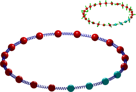
As a first example, we consider the most basic classical model for the vibration in a solid, namely a set of particles of mass $m$, arranged on a ring and connected to their two neighbors by harmonic springs, see Fig. 1. The Hamiltonian of the system reads

$$H=\sum_{i=1}^{N}\frac{p_{i}^{2}}{2m}+\frac{m\Omega^{2}}{2}\sum_{i=1}^{N}(x_{i}-x_{i+1})^{2},$$ (1)

where $x_{i}$ and $p_{i}$ are the displacement and momentum of the $i$th oscillator, $m\Omega^{2}$ is the spring constant and $N$ is the total number of particles. For convenience, $m$ and $\Omega$ are set to $1$ and all quantities such as momenta and displacements are taken to be dimensionless. The positions are constrained to lie on a circle. Changing to normal-mode coordinates $\{P_{k},X_{k}\}$, the Hamiltonian reads $H=(1/2)\sum_{k=0}^{N-1}\left(P_{k}^{2}+\omega_{k}^{2}X_{k}^{2}\right)$ where $\omega_{k}=2|\sin\pi k/N|$. The motion of each set of coordinates $\{P_{k},X_{k}\}$ is described by a single sinusoidal oscillation and is decoupled from the motion of all other sets. Clearly, this classical system is integrable which allows us to compute numerically the coordinates and momenta of the oscillators without introducing systematic or cumulative errors. To this end, we transform the set of values of $\{x_{1},\ldots,x_{N},p_{1},\ldots,p_{N}\}$ at time $t=0$ to their corresponding normal-mode values, use the simple sinusoidal dependence of the latter to obtain their values at any point $t$ in time, and use the inverse transformation to find the values of $\{x_{1},\ldots,x_{N},p_{1},\ldots,p_{N}\}$ at time $t$. This whole procedure is numerically exact, up to machine precision.

Figure 1: Picture of the harmonic oscillator (large) and magnetic moment (small) models, subject to periodic boundary conditions. Particles are connected by harmonic springs or carry a magnetic moment that interacts with its nearest neighbors. The blue (red) colored particles belong to the subsystem (environment).

As a second example, we consider a ring of classical magnetic moments, their total energy given by the Hamiltonian Fisher (1963)

$$H=-J\sum_{i=1}^{N}\mathbf{S}_{i}\cdot\mathbf{S}_{i+1},$$ (2)

where $\mathbf{S}_{i}$ is a $3$-dimensional unit vector, representing the magnetic moment of a particle at lattice site $i$, $J$ defines the energy scale which we set equal to $1$ in our numerical work and $N$ is the total number of moments. The equation of motion of these moments reads

$$\frac{d}{dt}\mathbf{S}_{i}=\frac{\partial H}{\partial\mathbf{S}_{i}}\times\mathbf{S}_{i}=-J\mathbf{S}_{i}\times\left(\mathbf{S}_{i-1}+\mathbf{S}_{i+1}\right),$$ (3)

which obviously is nonlinear. Nevertheless, Eq. (3) admits a harmonic-wave solution $\mathbf{S}_{i}(t)=(\mathbf{a}\cos\theta_{i}+\mathbf{b}\sin\theta_{i})\cos\phi+\mathbf{c}\sin\phi$, where $\theta_{i}=ip-\omega t$, $\omega=2(1-\cos p)\sin\phi$, $\phi$ and $p$ are real constants, and $(\mathbf{a},\mathbf{b},\mathbf{c})$ form a right-handed set of orthogonal unit vectors Lakshmanan et al. (1976); Roberts and Thompson (1988). More generally, Eq. (3) has simple analytical solutions for $N=2$ and $N=3$ Steinigeweg and Schmidt (2009). The motion of $N=4$ magnetic moments arranged on a ring is regular Steinigeweg and Schmidt (2009). For $N>4$, the system exhibits chaotic motion Steinigeweg and Schmidt (2009), except for special initial conditions such as the spin-wave and soliton solutions Schmidt et al. (2011). We integrate the nonlinear equations of motion using a fourth-order Suzuki-Trotter product-formula method which conserves (1) the volume of the phase space, (2) the length of each magnetic moment and (3) the total energy Krech et al. (1998). Due to the chaotic character of the motion of the magnetic moments, their trajectories are unstable with respect to rounding and time-integration errors. Nevertheless, the numerical method used guarantees that the motion of the magnetic moments strictly conserves the energy, as required for a microcanonical ensemble simulation.

Figure 2: Left: Poincaré-type map of the differences $\Delta X=(x_{0}-x_{1})/2$ and $\Delta P=(p_{0}-p_{1})/2\sqrt{2}$ for a ring of $N=512$ oscillators. This system is integrable. Right: Poincaré-type map of the differences $\Delta X^{\prime}=S^{x}_{1}-S^{x}_{2}$ and $\Delta P^{\prime}=S^{z}_{1}-S^{z}_{2}$ for a ring of $N=512$ magnetic moments. This system is chaotic Steinigeweg and Schmidt (2009). Each graph contains 5000 points.

In our numerical work, the initial values of the coordinates or magnetic moments are generated by standard Monte Carlo methods Landau and Binder (2000), see the Supplementary Information.

In the normal-mode representation, each of the oscillators traces out an ellipse in the $(X_{k},P_{k})$ plane. However, in the original coordinates, this simplicity is lost as illustrated by the Poincaré map shown in Fig. 2(left). Clearly, it is difficult to detect some regularity in this map. Moreover, this map is very similar to Fig. 2(right), the Poincaré-type map of a one-dimensional classical model of magnetic moments. This similarity exists in spite of the fact that the oscillator system is not chaotic.

The whole system is divided into two parts, a subsystem with $N_{S}$ particles and an environment with $N_{E}=N-N_{S}$ particles. The Hamiltonian is written as $H=H_{S}+H_{E}+H_{SE}$, where $H_{S}$ ($H_{E}$) denotes the energy of the subsystem (environment) and $H_{SE}$ denotes the energy due to the interaction of the subsystem with the environment. Thus, in the case of particles arranged on a ring, $H_{S}$ and $H_{E}$ are open chains of particles, and $H_{SE}$ only contains two terms of the form $(x_{i}-x_{i+1})^{2}$ or $\mathbf{S}_{i}\cdot\mathbf{S}_{i+1}$ for the oscillator and magnetic system, respectively.

Figure 3: Time evolution of the energy per particle $E_{S}/N_{S}$, as obtained from a chain of $N_{S}=80$ particles embedded in a ring of $N=512$ particles. Initially, the subsystem of $N_{S}=80$ particles is put in its ground state and the configuration of the environment of $N_{E}=N-N_{S}=432$ particles is drawn randomly from its canonical distribution at temperature $T=1$. Red line: energy per particle of the subsystem; horizontal black line: energy per particle of the whole system. Main figure: the energy of the oscillators in the subsystem quickly relaxes to the average energy of the whole system. The inset shows the corresponding data for the spin system.

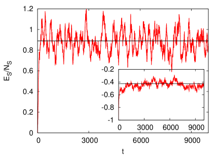
We first study the dynamic evolution of the subsystem when it is brought in contact with the environment. Initially, using one of the procedures described in the Supplementary Information, the subsystem and environment are prepared such that they have a different energy. As the whole system evolves in time, strictly conserving the total energy, we monitor the energy of the subsystem as a function of time. Some representative results are shown in Fig. 3, for both the harmonic oscillator and magnetic moment model. From Fig. 3, it is clear that for both models, the energy of the subsystem $E_{s}$ rapidly approaches the average energy of the whole system.

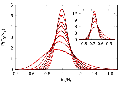
Having established that the Newtonian equation of motion drives the subsystem and environment to a common equilibrium state, the next step is to study the distribution of the subsystem energy. After the relaxation to the equilibrium state, we monitor the energy $E_{S}$ of the subsystem at regular time intervals and construct a (normalized) frequency distribution $P(E_{S})$ of the energy of the subsystem, see Fig. 4.

The hypothesis that Newtonian dynamics causes the subsystem to visit points in phase-space with frequencies that match with those of the canonical probability distribution can now be tested as follows. According to statistical mechanics, the distribution of energy in the canonical ensemble is given by Greiner et al. (1997)

$$p(E)=g(E)e^{-E/T}/Z,$$ (4)

where $T$, $E$, $g(E)$ and $Z$ are the temperature (in units of $k_{B}=1$), the total energy, the density of states and the partition function, respectively Greiner et al. (1997). The function $p(E)$ has a maximum at some energy $E^{\ast}$, the most probable energy at the temperature $T$ Greiner et al. (1997). In the vicinity of $E^{\ast}$, we have Greiner et al. (1997)

$$p(E)=Ae^{a_{2}(E-E^{\ast})^{2}+a_{3}(E-E^{\ast})^{3}+a_{4}(E-E^{\ast})^{3}+\ldots},$$ (5)

where $A$ is a normalization constant and the coefficients $a_{n}=(1/n!)\partial^{n}S(E)/\partial E^{n}|_{E^{\ast}}$ are determined by the microcanonical entropy $S(E)$ of the subsystem Greiner et al. (1997).

For the two models considered in this paper, the coefficients $a_{n}$ are simple functions of $T$ and $N_{S}$ (see Supplementary Information). Therefore, using $T$ and $E^{\ast}$ as adjustable parameters a fit of Eq. (5) to the histogram $P(E_{s})$ obtained from the dynamical evolution of the subsystem yields an estimate of the temperature $T_{S}$ of the subsystem. As shown in Fig. 4, the simulation data for $P(E_{S})$ (red lines) and fitted $p(E)$ (black lines) are in excellent agreement, for both models alike. In the thermodynamic limit ($N_{E}\rightarrow\infty$ before $N_{S}\rightarrow\infty$), all but the quadratic term in the exponential can be neglected and the distribution is Gaussian Greiner et al. (1997). Therefore, for large $N_{S}$, $T_{S}$ and $E^{\ast}$ can be obtained by fitting a Gaussian to $P(E_{S})$ but from Fig. 4, it is clear that for small subsystem sizes, $P(E_{s})$ deviates significantly from a Gaussian. However, taking into account the higher-order terms in the expansion Eq. (5), the agreement between simulation data and the prediction of statistical mechanics is excellent. Repeating the simulations with different initial conditions (including different initial energies for the subsystem or the environment) strongly suggests that this agreement is generic.

Figure 4: The distribution $P(E_{S})$ as a function of the energy per particle $E_{S}/N_{S}$ for different sizes $N_{S}$ of the subsystem, as obtained from the solution of Newtonian equations of motion for the oscillator system. Red lines: $N_{S}=20,40,60,80,100,120,160,200$ (broad to narrow) and $N=65536$. Black lines: probability distribution predicted by statistical mechanics Eq. (5) using all terms up to $(E-E^{\ast})^{8}$. In all cases, the initial energy of the environment corresponds to a temperature $T=1$ and the number of samples is $4\times 10^{6}$. The inset shows the corresponding data for the spin system for $N_{S}=20,40,60,80,100$ and $N=2000$, with the initial energy of the environment corresponding to $T=0.329$ and the number of samples is $10^{6}$.

If the estimate $T_{S}$ is indeed the temperature of the subsystem, the second central moment of $P(E_{S})$ should be related to the specific heat of the subsystem. To check this, we define

$$C_{S}\equiv\frac{\langle E_{S}^{2}\rangle-\langle E_{S}\rangle^{2}}{T_{S}^{2}}$$ (6)

where $\langle E_{S}\rangle$ and $\langle E_{S}^{2}\rangle$ are the first and second moment of $P(E_{S})$, respectively. Our numerical results (see Supplementary Information) are in excellent agreement with canonical ensemble theory.

As a conclusive test, we perform microcanonical Monte Carlo simulations for both models (see Supplementary Information) and obtain the distributions $P_{\mathrm{mc}}(E_{s})$ of the subsystems. The microcanonical Monte Carlo simulation generates statistically independent configurations of the whole system strictly according to the microcanonical distribution but samples the phase space in a completely different manner than does Newtonian dynamics. The Kullback-Leibler distance $D(P_{\mathrm{mc}}(E_{s});P(E_{s}))$ is a convenient measure to quantify the difference between the two distributions $P_{\mathrm{mc}}(E_{s})$ and $P(E_{s})$ Press et al. (2003). In all cases, we find that the difference between $P_{\mathrm{mc}}(E_{s})$ and $P(E_{s})$ is very small (see Supplementary Information). For instance, for the system of oscillators with $N_{S}=20$, $N=65536$ and $10^{8}$ samples, we find that $D(P_{\mathrm{mc}}(E_{s});P(E_{s}))\approx 4\times 10^{-2}$, indicating that the probability that the two distributions are different is very small.

Having established that the interaction of the environment with the subsystem causes both systems to equilibrate and also drives the latter to its canonical state, it becomes possible to derive from the Newtonian dynamics alone, estimates for the equilibration time. To this end we express the equilibration time estimated from the simulations in physical units. Typical frequencies of vibration in a solid are of the order of $10^{11}$Hz. Using this number to set the scale of the frequency $\Omega$ in our model, we find that equilibration takes of the order of $10^{-9}\;\mathrm{s}$. Similarly, for the system of magnetic moments, a realistic value of $J/k_{B}$ is of the order of $10\;\mathrm{K}$, yielding an equilibration time of the order of $10^{-8}\;\mathrm{s}$. Classical spin systems with Hamiltonians that encode frustration and/or disorder of regular or random kind are however expected to exhibit larger, possibly much larger equilibration time scales. The dynamical properties for subsystems of such theories under Newtonian evolution are beyond the scope of the present work.

Even though the subsystems and the environments which we have simulated are very small in the thermodynamic sense, the subsystem and environment equilibrate on a nanosecond time scale. Therefore, for an isolated nanoparticle of even a few thousand atoms, an experimental probe that concentrates on only a few of those atoms should yield data that follows the canonical distribution.

Calculations have been performed at JSC under project JJSC09. MIK acknowledges financial support from FOM, the Netherlands. MAN is supported in part by the National Science Foundation. This work is partially supported by the Mitsubishi Foundation (SM) and NCF, the Netherlands (HDR).

References

- Kubo et al. (1985) R. Kubo, M. Toda, and N. Hashitsume, Statistical Physics II: Nonequilibrium Statistical Mechanics (Springer-Verlag, New York, 1985).
- Greiner et al. (1997) W. Greiner, L. Neise, and H. Stöcker, Thermodynamics and Statistical Mechanics (Springer-Verlag, New York, 1997).
- Schuster (1995) H. G. Schuster, Deterministic Chaos: An Introduction (Wiley-VCH, New York, 1995).
- Zaslavsky (1985) G. M. Zaslavsky, Chaos in Dynamic Systems (Harwood Academic Publishers, New York, 1985).
- Sagdeev et al. (1988) R. Z. Sagdeev, D. A. Usikov, and G. M. Zaslavsky, Nonlinear Physics: From the Pendulum to Turbulence and Chaos (Harwood Academic Publishers, New York, 1988).
- Prigogine (1980) I. Prigogine, From Being to Becoming: Time and Complexity in the Physical Sciences (W. H. Freeman & Co, 1980).
- Fermi et al. (1955) E. Fermi, J. Pasta, and S. Ulam, Los-Alamos internal report, Document LA-1940 (1955).
- Ford (1992) J. Ford, Phys. Rep. 213, 271 (1992).
- Gallavotti (2008) G. Gallavotti, The Fermi-Pasta-Ulam Problem: A Status Report (Lecture Notes in Physics) (Springer-Verlag, 2008).
- Porter et al. (2009) M. Porter, N. Zabusky, B. Hu, and D. Campbell, American Scientist 97, 214 (2009).
- Hemmer et al. (1958) P. C. Hemmer, L. C. Maximon, and H. Wergeland, Phys. Rev. 111, 689 (1958).
- Mazur and Montroll (1960) P. Mazur and E. Montroll, J. Math. Phys. 1, 70 (1960).
- Ford and Waters (1963) J. Ford and J. Waters, J. Math. Phys. 4, 1293 (1963).
- Gibbs (1902) J. Gibbs, Elementary Principles in Statistical Mechanics (Yale University, New Haven, CT, 1902).
- Tolman (1927) R. Tolman, Statistical Mechanics with Applications to Physics and Chemistry (ACS Monograph Series 32, 1927).
- Uline et al. (2008) M. Uline, D. Siderius, and D. Cortial, J. Chem. Phys. 128, 124301 (2008).
- Eastwood et al. (2010) M. Eastwood, K. Stafford, R. Lippert, M. Ø. Jensen, P. Maragakis, C. Predescu, R. Dror, and D. Shaw, J. Chem. Theory Comput. 6, 2045 (2010).
- Steinigeweg and Schmidt (2009) R. Steinigeweg and H.-J. Schmidt, Math. Phys. Anal. Geom. 12, 19 (2009).
- Fisher (1963) M. E. Fisher, Am. J. Phys. 32, 343 (1963).
- Lakshmanan et al. (1976) M. Lakshmanan, T. W. Ruijgrok, and C. J. Thompson, Physica A 84, 577 (1976).
- Roberts and Thompson (1988) J. A. G. Roberts and C. J. Thompson, J. Phys. A: Math. Gen. 21, 1769 (1988).
- Schmidt et al. (2011) H.-J. Schmidt, C. Schröder, and M. Luban, J. Phys.: Condens. Matter 23, 386003 (2011).
- Krech et al. (1998) M. Krech, A. Bunker, and D. Landau, Comp. Phys. Comm. 111, 1 (1998).
- Landau and Binder (2000) D. P. Landau and K. Binder, A Guide to Monte Carlo Simulation in Statistical Physics (Cambridge University Press, Cambridge, 2000).
- Press et al. (2003) W. H. Press, B. P. Flannery, S. A. Teukolsky, and W. T. Vetterling, Numerical Recipes (Cambridge University Press, Cambridge, 2003).