How big is too big? Critical Shocks for Systemic Failure Cascades

C. J. Tessone, A. Garas, B. Guerra, F. Schweitzer

1 Introduction

Current research on systemic risk can be roughly divided into two different strands each one having its own focus: (i) the probability of extreme events which can cause a breakdown of the system, (ii) the mechanisms which can amplify the failure of a few system elements, to cause a failure cascade of the size of the system. The former line of research assumes that systemic risk is caused by external events, e.g. big earthquakes, tsunamis, or meteor impacts. Thus, in addition to the likelihood of extreme events, another interesting question regards the response of the system to such perturbations, i.e. its capability to absorb shocks of a given size. The latter research area, on the other hand, sees systemic failure as an endogenous feature that basically emerges from the non-linear interaction of the constituents, i.e. how they redistribute, and possibly amplify, load internally.

In both approaches, the likelihood of a systemic breakdown can only be determined by considering the internal dynamics of system elements, denoted as agents in this paper, such as their capacity to resist shocks, their time-bound interaction with neighbors, their dependence on macroscopic feedback mechanisms, such as coupling to the macroscopic state of the system. Only in rare cases the dynamics of systemic risk can be reduced to mere topological aspects, such as the diversity in the number of neighbors, the role of hubs, etc.. In this paper, we combine the two research questions mentioned above: on the one hand, we are interested in the critical size of an external shock that may lead to collapse of the system. At the same time, we address that such critical values depend on the safety margins of the system elements, and the details of their interaction when redistributing load internally. We also investigate how these cascading dynamics are affected by the structural features of the network (level of connectivity, topological heterogeneities)and by individual properties of the agents, such as the probability distributions of the failure thresholds. Such insights can directly benefit a robust system design by means of individualization of agents (i.e. designing agents with optimal heterogeneity).

Given the importance of such problems for social, economical and technological systems, the topic is already discussed in a wide range of scientific literature. Some modeling framework were recently proposed [Lorenz2009b, Watts2002SimpleModelof, dodds2004universal]. The complex network approach was also used to describe cascading processes in power grids and in Internet services [motter2002cascade, crucitti2004model], and was also applied to data storage services [rossi2009]. Importantly, similar agent-based approaches were developed to model avalanche defaults among financial institutions [Battiston2009a, gai2010contagion].

Our paper is organized as follows: in the next section we introduce the agent-based model studied, determining e.g. agent’s fragility and agents’ interaction by means of a load redistribution mechanism. This allows us to define a measure for systemic risk on the macroscopic level. In Section 3 we develop an analytical framework that allows us to unveil the dynamics of systemic risk based on cascading processes. In Section 3.2, we discuss the critical conditions for systemic risk to emerge. Later, in the Section 3.3, we study when agents can be considered as systemic by their importance. The paper finishes with some conclusions in Section 4, which also allow for a generalized picture of how to prevent systemic risk.

2 Analytical approach to systemic risk

2.1 Description of the model

Net fragility

In a recent paper [Lorenz2009b], a framework to model systemic risk by means of an agent-based approach was developed. In this framework, each agent $r$ is characterized by three individual variables: a discrete variable $s_{r}(t)\in\{0,1\}$, which describes its state at a discrete time $t$, i.e. $s_{r}(t)=0$ for an operating state and $s_{r}(t)=1$ for a failed state, and two continuous variables, the threshold $\theta_{r}$ and load $\phi_{r}$. The threshold is assumed to describe the individual ‘capacity’ of an agent: it defines how much load an agent can carry before it fails. On the other hand, the variable $\phi_{r}$ describes the load which is exerted on an agent.

We note that while the load can change in time e.g. through systemic feedback, it further depends on the state of other agents $\underline{s}$ and on the network of interactions, described by the adjacency matrix $A$. Written this way, the load also depends on how it is exchanged between agents. A special case will be discussed below. We define that agent $r$ fails if its net fragility $z_{r}(t)$,

$$z_{r}(t)=\phi_{r}(t,A,\underline{s})-\theta_{r},$$ (1)

is equal or larger than zero. I.e, in a deterministic model, the dynamics of an agent is given by

$$s_{r}(t+1)=\Theta\big{(}z_{r}(t)\big{)},$$ (2)

where $\Theta(\cdot)$ is the Heaviside function. Certainly, the dynamics only depends on the net fragility, i.e. on the relative distance between load and threshold. Nevertheless, a distinction between these two individual variables is very useful, as it allows us to conceptually distinguish between internal and external influences on the failure.

Systemic risk

We now define the important measure of systemic risk. We define it as the fraction of failed agents at any point in time. For a system composed of $N$ agents, it reads

$$X(t)=\frac{1}{N}\sum_{r}s_{r}(t)=\int_{0}^{\infty}p_{z(t)}\big{(}z\big{)}dz;$$ (3)

$p_{z(t)}\big{(}z\big{)}$ represents the density of agents with a net fragility $z$ at time $t$; the integral runs over the agents whose net fragility is positive. Failures in a subset of agents will result in cascading processes over the network of interaction, which results in changes of the fragility of other agents in the course of time. This can be expressed by the recursive dynamics $p_{z(t+1)}=\mathcal{F}(p_{z(t)})$, where $\mathcal{F}$ is some function that describes how the load of failing agents is redistributed depending on the interaction mechanisms. With this, by specifying the initial condition $p_{z(0)}$, it is possible to compute $X(t)$ for a deterministic dynamics.

In Ref. [Lorenz2009b], $X(t)$ was calculated by making suitable assumptions about the distribution of the net fragility, $p_{z}(t)$, the initial conditions $p_{z(0)}$, and for the particular case of a fully connected network – i.e. each agent interacts with everyone else. Specifically, an initial condition $p_{z(0)}\sim\mathcal{N(\bar{\theta},\sigma)}$, was used; i.e. the initial fragility of agents is normally distributed with a mean $\bar{\theta}$ and standard deviation $\sigma$. This implies that the initial fraction of failed agents at time $t=0$ is given by $X(0)=\Phi_{\bar{\theta},\sigma}(0)$, where $\Phi_{\bar{\theta},\sigma}(0)$ denotes the cumulative function of the normal distribution. I.e. it gives the (normalized) number of agents with an initial net fragility (defined in Eq. (1)), equal or larger than zero. The authors calculated the size of cascades measured by the final fraction of failed agents for different interaction mechanisms. Remarkably, it was found that systemic risk depends on the variance $\sigma$ of the distribution $p_{z}(0)$ in a non-monotonous manner. This means, systemic risk can decrease if the agents become more heterogeneous, i.e. if their individual threshold becomes more different. On the other hand, for homogeneous agents characterized by the same threshold, a first-order phase transition was found between no systemic risk and complete failure.

Initial fragility

We use these previous findings as a reference point, but we will extend our model in different ways. First of all, instead of a normal distribution for the initial net fragility $z_{r}(0)=\phi_{r}(0)-\theta_{r}$, we assume a fixed relation between initial fragility $\phi_{r}(0)$ and threshold $\theta_{r}$:

$$\phi_{r}(0)=\alpha\theta_{r}\quad(r=1,\ldots,N;\;r\neq i).$$ (4)

The parameter $\alpha$ is a constant, equal for all agents. Only for one agent $i$, instead of the fixed relation (4), we define $\phi_{i}(0)=\phi_{\star}\geq\theta_{i}$. Thus, we consider that initially only one agent $i$, is at a critical condition, whereas with $\alpha<1$ all other agents are initially capable of handling the load assigned to them. I.e. different from the distribution of initial loads in [Lorenz2009b], we do not have an initial failure cascade. Instead, the initial condition for the systemic risk is simply $X(0)=1/N$.

The value $1-\alpha$ can then be regarded as the agent available capacity (or safety margin) before they fail if their load is increased. A fixed relation between fragility and threshold was first used in [motter2002cascade] to describe cascading processes in power grids and Internet (see also [crucitti2004model, Motter2004CascadeControland, CRUCITTI_cascades_power_grid]). It basically reflects the situation of many socio-technical systems in which the capacity of agents is usually ad hoc designed to handle the load, because limited by cost, under normal conditions. We will later vary the safety margin $1-\alpha$ to determine how the severity of cascading failures will depend on it.

Threshold distribution

With these considerations, only the threshold distribution $P(\theta)$ remains to be specified to complete the initial conditions. It is worth remarking that the capacities of the agents –in contrast with other studies found in the Literature so far– are decoupled from the topological artifacts of the network connecting them. Here we will use three different assumptions for both analytical calculations and computer simulations:

• a delta distribution $P(\theta)=\delta(\theta-\bar{\theta})$, where $\delta(\cdot)$ is the Dirac delta function, i.e. all agents have the same threshold $\bar{\theta}$,

• a uniform distribution $P(\theta)=U(\bar{\theta}-\sigma,\bar{\theta}+\sigma)$ with the mean $\bar{\theta}$ and the range $\sigma$, i.e. all agents have different, but comparable thresholds in the interval $[\bar{\theta}-\sigma,\bar{\theta}+\sigma]$. For all further calculations we define $\theta_{\mathrm{min}}=\bar{\theta}-\sigma$.

• a power-law distribution

  $$P(\theta)=\frac{\gamma-1}{\theta_{\mathrm{min}}^{1-\gamma}}\,\theta^{-\gamma}$$ (5)

  i.e. agents have thresholds that can differ by orders of magnitudes. As the normalization depends on the value $\theta_{\mathrm{min}}$, we assign its numerical value for our further calculations to be comparable with the minimum value of the uniform distribution, $\theta_{\mathrm{min}}=\bar{\theta}-\sigma$.

Agent interaction

In order to describe the agent interaction, we use the network approach in which agents are represented by nodes and interactions by links between agents. I.e., the network topology specifies which other agents a particular one interacts with. This can be statistically described by the degree distribution $P(k)$ for which we will use in this paper only $P(k)=\delta_{k_{r},K}$, i.e. a regular network, in which each agent interacts with $K$ other agents. The fully connected network is a special case with $K=N-1$.

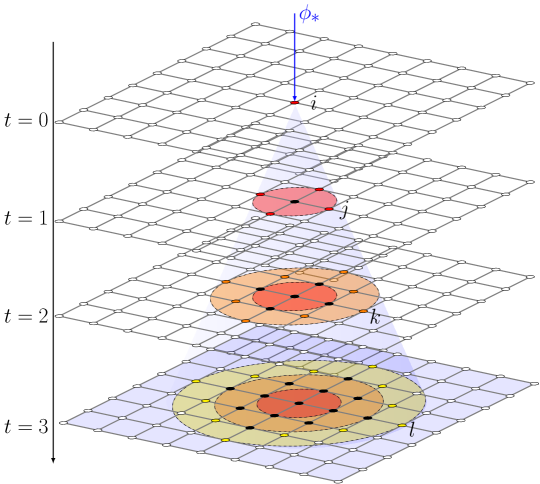
Secondly, we have to specify how agents interact through these links. Here, we assume a load redistribution mechanism in which the initially failing agent $i$ shares its load $\phi_{i}(0)\equiv\phi_{\star}$ equally among its $K$ neighboring agents (labeled $j$), see Fig. 1. That means for each of these agents, their own load $\phi_{j}(t)$ increases in the next time step $(t+1)$ by an amount of $\phi_{\star}/{K}$. If this addition leads to a positive net fragility $z_{j}(t)=\phi_{j}(t)-\theta_{j}$, agents $j$ fail as well and redistribute their load $\phi_{j}(t+1)$ equally to their $K$ neighboring agents, and so on.

Figure 1: Regular lattice with $K=4$, where agent $i$ is hit initially ($t=0$) by an external shock of size $\phi_{\star}$. If $i$ fails, it distributes this load to its $K$ nearest neighbors in the next time step ($t=1$). If they fail, they distribute their load to their $K$ nearest neighbors in the next time step ($t=2$) , which are the $2K$ second nearest neighbors of $i$, etc..

Cascade sizes

This way, failure cascades can occur in the course of time, and we are interested in their relative size and the probability distribution of their occurrence, $P(X(t))$. For this calculation, which will be done in Sect. 3.2, we define the fraction $f(t)$ of failing agents at each time step $t$ and the number $F(t)$ of failing agents during the same time interval as:

$$f(t)=\frac{1}{K(t)}\sum_{r=1}^{N}s_{r}(t)-s_{r}(t-1)\;;\quad F(t)=K(t)\,f(t)\;;\quad f(0)=1.$$ (6)

$K(t)$ gives the number of agents that are hit by the cascade at time $t$, i.e. they are located in the $t$–th neighborhood of agent $i$ which failed initially. Hence, with the model of Fig. 1 in mind, $K(t)$ is the number of agents that can potentially fail during time step $t$. Dependent on the topology of the regular network, there are two limiting cases to express how $K$ grows in time. $K(t)\propto K\,t$ holds in regular networks, where the interface grows linearly with distance. On the other hand, for Bethe lattices, tree-like structures and random topologies in which loops are neglected [Watts2002SimpleModelof], the number of nodes at distance $t$ is $K(t)=K^{t}$.

Using the definition (6), we can calculate the size of the cascade at time $t$, which is equal to the systemic risk $X(t)$ as:

$$X(t)=\frac{1}{N}\sum_{\tau=0}^{t}F(\tau)=\frac{1}{N}\sum_{\tau=1}^{t}K(\tau)\,f(\tau).$$ (7)

In general, Eq. (7) cannot be solved analytically. However, in the following sections we will derive analytical expressions for $f(t)$, assuming different distributions of agents’ thresholds.

Finite versus infinite cascades

According to the definitions above, a total failure occurs if $X(t)=1$. In a finite system, this will happen at a finite time $t^{\prime}$, while in an infinite system this final state is reached only asymptotically, $t^{\prime}\to\infty$. However, in a finite system a cascade can stop even for $X(t)<1$ if the potential number of failing agents reaches the system size at a given time $t^{\circ}$,

$$\sum_{t=0}^{t^{\circ}}K(t)\geq N.$$ (8)

Yet, there is a third case to be considered, namely that the cascade stops at a finite time $t^{\star}$, even if $X(t)<1$ and $t<t^{\circ}$, simply because the redistribution of loads to the nearest neighbors does not cause further failure. This is expressed by the condition $f(t^{\star})=0$.

We will refer to an “infinite” cascade if $X(t^{\prime})=1$, which means every agent in the system has failed. On the other hand, a “finite” cascade occurs either if it stops at time $t^{\star}<t^{\circ}$, or if the redistribution of load has reached the system size, Eq. (8), without causing all agents to fail. Consequently, finite cascades stop at time $t^{\prime}=\min(t^{\circ},t^{\star})$. We note that, according to our definition, Eq. (7), systemic risk refers to finite cascades as well, not just to $X\to 1$. Precisely, we are interested in the distribution $P(X(t^{\prime}))$, i.e. the density of failed agents at the time by which cascades end regardless of the cause for that.

Network capacity

In order to put the size of the initial shock $\phi_{\star}$ into perspective, we refer to the total capacity of the network to absorb shocks, which depends on the safety margin $(1-\alpha)$, the total number of nodes, and the threshold distribution $P(\theta)$. Thus, the capacity $Q$ that the system could a priori absorb during the cascade is simply given by

$$Q=N(1-\alpha)\int d\theta\,\theta\,P(\theta).$$ (9)

If the threshold distribution has a defined mean value, $\bar{\theta}$, this expression reduces to $Q=N(1-\alpha)\,\bar{\theta}$. On the other hand, for a normalized power-law distribution with a minimum threshold value $\theta_{\mathrm{min}}$, the mean value is only defined for $\gamma>2$. For $\gamma\leq 2$, a simple argument [Tessone2010] shows that for a finite system the expected value can still be computed. The result is

$$\frac{Q}{N(1-\alpha)}=\left\{\begin{array}[]{lll}\theta_{\text{min}}&\left[\frac{\displaystyle\gamma-1}{\displaystyle\gamma-2}+\frac{\displaystyle N^{2-\gamma}}{\displaystyle 2-\gamma}\right]&\text{if}\,\gamma\leq 2\\ \theta_{\text{min}}&\left[\frac{\displaystyle\gamma-1}{\displaystyle\gamma-2}\right]&\text{if}\,\gamma>2\end{array}\right..$$ (10)

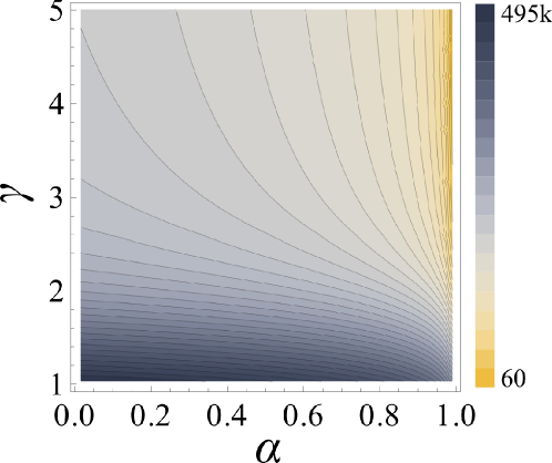
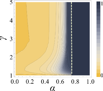
It is worth noticing that for the delta threshold distribution, the uniform (with $\bar{\theta}\sim\sigma$) and the power-law distribution with $\gamma>2$, the network capacity $Q$ is of the same order of magnitude. In Fig. 2 we show the network capacity $Q$ for the power-law distribution as a function of $\gamma$ and $\alpha$. Precisely, it gets the same numerical value in all three cases cases, $Q=Q_{u}$, if $\gamma=1.5$ and $\bar{\theta}=2\theta_{\mathrm{min}}$, as used for the numerical calculations. However, for the power law distribution with $\gamma\leq 2$, the network capacity becomes much larger than in the three other cases because of the additional dependence of the number of agents, $N^{2-\gamma}$. Choosing $\gamma=1.5$ for the numerical calculations later implies that, compared to the uniform case, we have $Q\propto\sqrt{N}Q_{u}$.

In this paper, depending on the magnitude of the initial shock, we distinguish between two different regimes:

(i) EEE – the extreme exogenous event resulting in a very large $\phi_{\star}$ which is of the order of $Q$, i.e. much larger than the capacity of the initially failing agent (or the average capacity $\bar{\theta}$ of agents): $\phi_{\star}\sim Q\gg\bar{\theta}$. In this case, there is no surprise that agents involved in the redistribution of load will fail, at least in an early phase. Hence, we are mostly interested in the conditions under which cascades may stop before they have reached the size of the system.

(ii) RIE – the random internal event, which assumes that initially one randomly chosen agent $i$ faces a load $\phi_{\star}$ that is slightly larger than its own capacity $\theta_{i}$, drawn from the distribution $P(\theta)$, i.e. $\phi_{\star}\sim\bar{\theta}\ll Q$. This is likely to happen by a random fluctuation of the load $\phi_{i}$ that exceeds the threshold, rather than a big impact on the system. In this case, we are interested in the conditions under which cascades occur at all.

Figure 2: Contour plot showing the network capacity $Q$ as a function of $\alpha$ and $\gamma$, for a network with $N=1000$ nodes having power-law threshold distribution with a minimum threshold value $\theta_{\mathrm{min}}=0.5$.

2.2 Conditions for failing nearest neighbors

We assume that, at $t=0$, a single randomly chosen agent $i\in 1\ldots N$ fails because of an initial shock, i.e. $\phi_{i}(0)\equiv\phi_{\star}\geq\theta_{i}$. According to the redistribution mechanism described above, this failure will increase the fragility of the nearest neighbors of $i$, labeled $j\in nn(i)$ (see Fig. 1). Agent $j$ can fail if its net fragility becomes positive, i.e.:

$$\phi_{j}(1)=\phi_{j}(0)+\frac{\phi_{\star}}{K}\geq\theta_{j},$$ (11)

which together with Eq. (4) leads to the critical condition for the failure of agent $j$,

$$\theta_{j}\leq\theta_{(1)}^{c}(\phi_{\star})=\frac{\phi_{\star}}{K(1-\alpha)}.$$ (12)

Here $\theta_{(1)}^{c}(\phi_{\star})$ defines the critical threshold for the first-order neighborhood of agent $i$, or the critical threshold at time $t=1$, respectively. Agents with a threshold between $\theta_{\mathrm{min}}$ and $\theta_{(1)}^{c}$ will fail, hence the fraction of failing agents at time $t=1$ reads:

$$f(1)=\int_{\theta_{\mathrm{min}}}^{\theta^{c}_{(1)}(\phi_{\star})}d\theta P(\theta).$$ (13)

This fraction depends on the threshold distribution $P(\theta)$, so explicit calculations will be given in the next Section. At the moment we just assume that at least one agent $j$ has failed, i.e. there will be a cascade to the next neighborhood (cf. Fig. 1).

Let us denote failing agents in the first step by $j^{\star}\in nn(i)$. Their load $\phi_{j}^{*}(t=1)>\theta_{j}$ will be redistributed to their nearest neighbors labeled $k\in nn(j^{\star})$. Following the reasoning used for Eq. (11), we obtain for the load of agents $k$ at time $t=2$: $$\phi_{k}(2)=\phi_{k}(1)+\sum_{j^{\star}\in nn(k)}\frac{\phi_{j^{\star}}(1)}{K}=\alpha\theta_{k}+\frac{1}{K}\sum_{j^{\star}\in nn(k)}\left(\phi_{j^{\star}}(0)+\frac{\phi_{\star}}{K}\right).$$ (14) The summation is performed over the whole set of failed agents $j^{*}$ that belong to the neighborhood of $k$, their load being $\phi_{j^{\star}}(0)=\alpha\theta_{j^{*}}$.

The exact amount of agents $j^{\star}\in nn(k)$ depend on the topological properties of the network considered. For example, in square and hexagonal lattices, some second nearest neighbors of $i$, i.e. agents $k$, have more than one link to agents $j$ in the nearest neighborhood. E.g. for the hexagonal lattice, half of the agents at level $k$ have two links to agents $j$, whereas the other half has only one. In general, for regular lattices, this number will be between one or two. In this paper, we will restrict our analysis to the case of a single failing node $j^{\star}$ in the neighborhood of $k$ which is the case for Bethe lattices or sparse random regular networks [construction]. The theory can be extended for other regular geometries in a straight-forward manner. With this considerations in mind, Eq. (14) becomes $$\phi_{k}(2)=\alpha\theta_{k}+\frac{1}{K}\left(\alpha\theta_{j^{\star}}+\frac{\phi_{\star}}{K}\right),$$ (15) From Eq.(15) we obtain the critical condition for the failure of agent $k$ if its net fragility becomes positive: $$\theta_{k}\leq\theta_{(2)}^{c}=\frac{\theta_{j^{\star}}+{\phi_{\star}}/{K}}{K(1-\alpha)}.$$ (16) This expression for the critical threshold at $t=2$, i.e. in the second-order neighborhood of $i$, is comprised of two redistribution processes. On the one hand those from agents $j^{\star}$ failing at $t=1$ and, on the other, the redistribution of the initial load $\phi_{\star}$ from agent $i$ failing at time $t=0$. The fraction of failed agents at time $t=2$ ($k\in nn(j^{\star})$) is then given by $$f(2)=\int_{\theta_{\min}}^{\theta^{c}_{(1)}(\phi_{\star})}d\theta_{(1)}P(\theta_{(1)})\int_{\theta_{\min}}^{\theta^{c}_{(2)}(\phi_{(1)})}P(\theta_{(2)})d\theta_{(2)},$$ (17) where $\theta^{c}_{(2)}(\phi_{(1)})$ indicates that the critical threshold at $t=2$ depends on the load of failing agents $j^{*}$ at time $t=1$, which does not need to be equal for every $j^{\star}$, but depends on the topology.

Using the same reasoning for the different time steps of the cascade, we obtain a general expression for the fraction of agents failing during time step $t$ (which are the neighbors of agents failing at $t-1$): $$f(t)=\int_{\theta_{min}}^{\theta^{c}_{(1)}(\phi_{\star})}d\theta^{(1)}P(\theta^{(1)})\cdots\int_{\theta_{min}}^{\theta^{(c)}_{(t-1)}(\phi_{(t-2)})}d\theta^{(t-1)}P(\theta^{(t-1)})\int_{\theta_{min}}^{\theta^{c}_{(t)}(\phi_{(t-1)})}d\theta^{(t)}P(\theta^{(t)}),$$ (18) The critical threshold $\theta^{c}(\phi_{(t)})$ at time $t$ depends on the load $\phi_{(t-1)}$ as follows: $$\theta_{(t)}\leq\theta^{c}_{(t)}=\frac{\phi_{(t-1)}}{K(1-\alpha)}.$$ (19) This is a recursive equation, i.e. $f(t)$ depends on the load redistributed by all the agents that failed along the path connecting the initially failing agent $i$ with agents failing at time $t$. However, Eq. (18) cannot be computed in general, thus, in the following sections, we will study some cases in which this equation can be reduced and solved.

2.3 Threshold approximation in the RIE and EEE regimes

Inequality (19) is an important result to understand the propagation of cascades, which holds for both regimes introduced above, the EEE regime, where the external shock dominates the dynamics, and the RIE regime, where small random events inside the first failing agents may trigger the cascade. For both, we are able to derive some general results even before specifying the threshold distribution $P(\theta)$.

In the RIE case, $\phi_{\star}\sim\bar{\theta}\ll Q$ the redistribution of loads, that means the network effect, plays the most important role. Note that pairs of agents connected through an edge have in general different capacities. If one of them fails, its neighbor is exposed to failure during the following time step. However, whether it fails or not will depend on: (a) the load redistributed from the failing agent; (b) its own capacity. Let us assume that if a agent with capacity $\theta_{(t-1)}$ fails, the total load induced on its neighbors is $\phi_{(t)}=\alpha\theta_{(t)}+{\theta_{(t-1)}}/{K}$. This assumption neglects the contribution of agents that failed before the time step $t-1$, which are terms of order $K^{-\tau}$, with $\tau\geq 2$. This implies that $\theta_{(t-1)}$ is the load distributed by the agent, i.e. it is exactly its capacity and not more. Thus, the largest capacity of the failing agent at time $t$, $\theta^{c}_{(t)}$, depends on the capacity of the agent that failed on the previous time step $t-1$, i.e.

$$\theta^{c}_{(t)}(\theta_{(t-1)})=\frac{\theta_{(t-1)}}{K(1-\alpha)}.$$ (20)

which is a lower bound for the failure condition, Eq. (19). This means that among all neighbors of the agents at layer $(t-1)$, those with a capacity lower than $\theta^{c}_{(t)}(\theta_{(t-1)})$ will fail.

With the assumption (20), the fraction of failing agents at time $t$ can be decomposed in terms of failure of two consecutive agents in a pair-wise approximation as follows:

$$f(t)=\int_{\bar{\theta}-\sigma}^{\theta^{c}_{(t-1)}}d\theta_{(t-1)}\,P(\theta_{(t-1)})\int_{\bar{\theta}-\sigma}^{\theta^{c}_{(t)}(\theta_{(t-1)})}d\theta_{(t)}\,P(\theta_{(t)}).$$ (21)

This approach differs from the previous mean-field approximation, in the following. Now, the net effect of the load redistributed by a failing agent is taken into account to determine the fraction of its neighbors that will fail in the next time step. Thus, this approximation entails information about the heterogeneity at the edge level. On the other hand, even in the EEE regime, $\phi_{\star}\sim Q\gg\bar{\theta}$, the role of the network still cannot be neglected. We are interested in the limit satisfying: (i) the load redistributed by the previously failed nodes cannot be totally neglected –i.e. $\alpha\sim 1$–; (ii) the main contribution to the load $\theta_{(t)}$ comes from $\phi_{\star}$ (i.e. from the initial load). We assume that at any point in time, there exists a critical threshold $\theta_{(t)}^{c}$ above which agents do not fail. In this case Eq. (19), becomes simply $\theta^{c}_{(t)}=\theta^{c}_{(t-1)}/[K(1-\alpha)]$. Then, the load of agents at a distance $t$ from agent $i$ is simply given by

$$\theta_{(t)}=\frac{{\phi}_{(t-1)}}{K(1-\alpha)}=\frac{{\phi_{\star}}}{[K(1-\alpha)]^{t}}.$$ (22)

which results in the critical threshold for the EEE regime:

$$\theta_{(t)}\leq\theta^{c}_{(t)}(\phi_{\star})=\frac{\phi_{\star}}{[K(1-\alpha)]^{t}}.$$ (23)

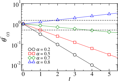
This gives the critical condition for the failing threshold of an agent that is hit by the cascade at time $t$ (i.e. it belongs to the $t$-th nearest neighborhood of the initially failing agent $i$). It nicely separates two effects that determine the severity of a cascade: (a) the size of the initial shock $\phi_{\star}$, (b) the number of neighbors to share the load and their respective safety margin, i.e. $K(1-\alpha)$. In the limit of large external shocks, and independent of further assumptions about the threshold distribution, the sequence of the critical thresholds $\theta^{c}_{(t)}$ crucially depends on the sign of the factor $K(1-\alpha)$. If $K(1-\alpha)>1$, the sequence $\theta^{c}_{(t)}$ will approach zero exponentially, i.e. with increasing distance from the initially failing agent, this condition will be more easily met. Hence, there should be a finite $t^{\prime}$ at which all reasonably chosen threshold values $\theta_{r}$ are larger than the critical threshold, which implies that the cascade stops. This is shown in Fig. 3 for the case of the uniform threshold distribution for different values of the safety margin $(1-\alpha)$. We can verify for the given set of parameters that for $\alpha=0.2$, and $\alpha=0.5$ the cascade stops right after $t=1$, while for $\alpha=0.7$ it stops after $t=3$. On the other hand, for $\alpha=0.8$ we see that the critical threshold is already at $t=3$ larger than any existing threshold, so the full cascade cannot be prevented.

While this is an intuitive and illustrative example, we will calculate analytically the exact time $t^{\prime}$ at which the cascade may stop, in the following section. We note again that due to the finite system size cascades may stop already at time $t^{\circ}$, which gives an additional limit.

Figure 3: Evolution of the critical threshold $\theta^{c}_{(t)}$ (note the $\log$ scale) versus the time step $t$ for the case of a uniform distribution with parameters $\bar{\theta}=1$ (dotted line), and $\sigma=0.5$ (dashed lines). The value of $K$ is set to four, while we used different values for the parameter $\alpha$.

3 Critical conditions for systemic risk

3.1 Analytical estimations of cascade sizes

Up to this point, we have derived a measure for systemic risk $X(t)$, Eq. (7) that is based on the fraction $f(t)$ of agents failing at a given time $t$. Failure cascades can propagate in the system if the net fragility of agents $\phi_{r}(t)-\theta_{r}$ is positive, i.e. if the load exceeds the capacity. While $\phi_{r}(t)$ becomes a function of the redistribution of loads in previous time steps, the capacity is determined by a threshold distribution function $P(\theta)$, for which we use three different specifications. Already the general framework outlined above allows us to expect “infinite” ($X\to 1$) and “finite” ($X<1$) cascades, where the latter can encompass the whole system or stop before. In the following, we will specify the conditions for these findings for the different threshold distributions.

Cascade size for homogeneous threshold

Let us start with the simplest case that all agents have the same threshold and the same number of neighbors. As stated above, there is a failing agent $i$ at $t=0$, for which $\phi_{i}(0)=\phi_{\star}$. Because of the homogeneous distribution, it can be noted that if an agent $r$ fails due to the failure of one of its neighbors, $r^{\star}$, then all the neighbors of $r^{\star}$ will fail as well. I.e. $f(t)=1$ if $f(t-1)=1$. Let $\phi_{(t)}$ be the load of agents at a distance $t$ of the initially failing agent at $t=0$ and let us assume that agents at a distance lower than $t$ already failed. Then, the load of agents in shell $t$ is

$$\phi_{(t)}=\alpha\bar{\theta}+\frac{\phi_{(t-1)}}{K}.$$ (24)

With the initial condition $\phi_{(0)}=\phi_{\star}$, this recursive equation can be easily solved, yielding

$$\phi_{(t)}=\alpha\bar{\theta}\,\frac{1-K^{-t}}{1-K^{-1}}+\frac{\phi_{\star}}{K^{t}}.$$ (25)

I.e., agents exposed to the redistribution of load at time $t$ will fail if $\phi_{(t)}>\bar{\theta}$. This equation allows to gain insight into the cascade mechanism. On the one hand, according to the above discussion of the EEE regime, infinite cascades can only be triggered if $K(1-\alpha)<1$, irrespective of the threshold distribution. This means a topological effect (the number and safety margin of neighbors among which the load is redistributed) decides about finite and infinite cascades.

On the other hand, when $K(1-\alpha)\geq 1$, the initial load $\phi_{\star}$ cannot (by itself) trigger an infinite cascade in the case of homogeneous threshold. I.e. even in the EEE regime, a cascade will only last $t^{\star}$ time steps, where $t^{\star}$ results from the failing condition $\theta^{(t^{\star})}\leq\phi_{(t^{\star})}$. From the condition $f(t^{\star})=0$, we can compute

$$t^{\star}=\frac{\log\left\{(1-K^{-1})\phi_{\star}-\alpha\bar{\theta}\right\}-\log\left\{(1-K^{-1})\bar{\theta}-\alpha\bar{\theta}\right\}}{\log K}.$$ (26)

As discussed before, the actual time $t^{\prime}$ at which the cascade stops is $t^{\prime}=\min(t^{\circ},t^{\star})$, where $t^{\circ}$ denotes the time where the cascade reaches the system size, Eq. (8).

Knowing $t^{\prime}$, we can further calculate the systemic risk according to Eq. (7), with $f(t)=1$, i.e. $F(t)=K(t)$ for $t\leq t^{\prime}$ and $F(t)=0$, otherwise. We find

$$X(t^{\prime})=\frac{K^{t^{\prime}-1}-1}{N(K-1)}$$ (27)

for a Bethe lattice or a tree with coordination number $K$ and

$$X(t^{\prime})\propto\frac{K(t^{\prime}+1)t^{\prime}}{N}$$ (28)

for a regular lattice, with the exact factor depending on the topology.

Cascade size for uniform threshold distribution

We now turn to the simplest case that allows some heterogeneity in the agent’s threshold, which is the uniform distribution $P(\theta)=U(\bar{\theta}-\sigma,\bar{\theta}+\sigma)$. The failing condition in Eq. (12) for the nearest neighbors still holds, but the question is how often we find thresholds below the critical limit:

$$f(1)=\int_{\bar{\theta}-\sigma}^{\theta_{(1)}^{c}}P(\theta)d\theta=\frac{\theta_{(1)}^{c}-(\bar{\theta}-\sigma)}{2\sigma}.$$ (29)

With $\theta^{c}_{(1)}$ given by Eq. (12) it turns out that the fraction of failing agents at the first time step is

$$f(1)=\frac{\phi_{\star}/[K(1-\alpha)]-(\bar{\theta}-\sigma)}{2\sigma}\quad\mathrm{if}\quad\phi_{\star}/(\bar{\theta}-\sigma)\geq K(1-\alpha)$$ (30)

and $f(1)=0$ otherwise. Regarding $f(t)$, we know from Eq. (18) that the fraction of failing agents at any time step crucially depends on the history of failed agents, i.e. the path connecting the initially failed agent with the currently failing one. Therefore, in general, the process is not solvable. There is the need of a simplifying assumption to break the integral expression in Eq. (18) into solvable parts.

For the EEE regime we use Eq. (23) and the underlying assumptions to obtain the closed equation,

$$f(t)=\int_{\bar{\theta}-\sigma}^{\theta_{c}(\phi_{(t-1)})}d\theta P(\theta)=\frac{1}{[K(1-\alpha)]^{t}}\frac{\phi_{\star}}{2\sigma}-\frac{\bar{\theta}-\sigma}{2\sigma}.$$ (31)

With this expression, we find from $f(t^{\star})=0$ the time at which the cascade stops for the uniform threshold distribution:

$$t^{\star}=\frac{\log(\phi_{\star})-\log(\bar{\theta}-\sigma)}{\log[K(1-\alpha)]}.$$ (32)

Again, the time at which the cascade ends is given by $t^{\prime}=\min(t^{\circ},t^{\star})$, with $t^{\circ}$ given by Eq. (8).

Considering instead the RIE regime, $\phi^{\star}\sim\bar{\theta}$, where redistribution effects play a mayor role, we use Eq. (21) and the underlying assumptions. Neglecting capacity-capacity correlations among agents, we find for the case of the uniform threshold distribution:

$$f(t)=\frac{\left(\theta^{c}_{(t-1)}-\bar{\theta}+\sigma\right)\left[\theta^{c}_{(t-1)}+\left[1-2K(1-\alpha)\right](\bar{\theta}-\sigma)\right]}{8\sigma^{2}\ K(1-\alpha)}.$$ (33)

The time at which the cascade stops is, as in the previous cases, given by the condition $t^{\prime}=\min(t^{\circ},t^{\star})$, where $t^{\star}$ is the first time step that verifies $f(t^{\star})=0$, and $t^{\circ}$ is the one defined in Eq. (8).

Cascade size for power-law threshold distribution

Now, we discuss the case where agent’s threshold follows a power-law distribution, Eq. (5), and can vary by orders of magnitude. With the same procedure as used before, we determine the fraction of failed agents during the initial cascade as

$$f(1)=\int_{\theta_{\mathrm{min}}}^{\theta_{(1)}^{c}}P(\theta)d\theta=1-\left(\frac{\phi_{\star}/\theta_{\mathrm{min}}}{K(1-\alpha)}\right)^{1-\gamma}.$$ (34)

So, cascades are obtained if $\phi_{\star}/\theta_{\mathrm{min}}\geq K(1-\alpha)$.

Considering first the EEE regime, we use the approximation given by Eq. (22) and find for the fraction of failing agents during time step $t$:

$$f(t)=1-\left(\frac{\phi_{\star}}{\theta_{\min}}\right)^{1-\gamma}\left[K(1-\alpha)\right]^{(\gamma-1)t}.$$ (35)

From $f(t^{\star})=0$, we calculate the time when the cascade stops as

$$t^{\star}=\frac{\log(\phi_{\star})-\log(\theta_{\mathrm{min}})}{\log[K(1-\alpha)]}.$$ (36)

Again, following our previous discussion, the cascade stops at $t^{\prime}=\min(t^{\star},t^{\circ})$.

In the RIE regime, on the other hand, Eq. , (21) has to be applied to the power law distribution, to yield

$$f(t)=1-\left(\frac{\theta_{\min}}{\theta^{c}_{(t-1)}}\right)^{\gamma-1}-\frac{[K(1-\alpha)^{\gamma-1}]}{2}\left[1-\left(\frac{\theta_{\min}}{\theta^{c}_{(t-1)}}\right)^{2\gamma-2}\right].$$ (37)

which, together with the failure condition of Eq. (20) provides a set of recursive equations, to be solved numerically.

3.2 Numerical results for the EEE regime

Size of finite cascades

The analytical results for $f(t^{\star})$ and $t^{\prime}=\mathrm{min}(t^{\star},t^{\circ})$ allow us now to calculate the systemic risk $X(t^{\prime})$ for the different threshold distributions, by varying system parameters such as the safety margin $(1-\alpha)$ or the network topology. In this section, we first concentrate on the EEE regime, where the external shock is comparable to the network capacity and much larger than the average threshold of an agent, $\phi^{\star}\sim Q\geq\bar{\theta}$.

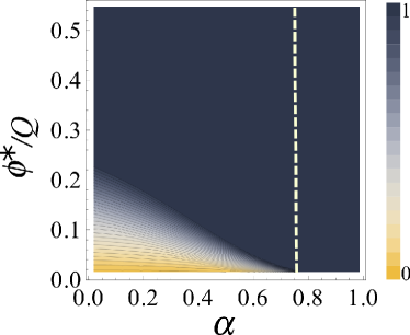
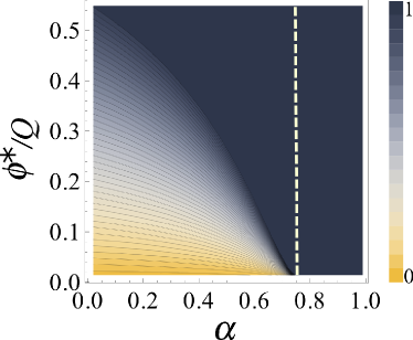
Figure 4: Systemic risk in a system with uniform threshold distribution with $\bar{\theta}=1$, and $\sigma=0.5.$ The contour plots show $X$ dependent on the initial shock $\phi_{\star}$ normalized to the network capacity $Q$ for different values of $\alpha$. Left: Bethe lattice, right: regular network. $K=4$, so the dashed line $K(1-\alpha)<1$ separates the region of “infinite” cascades, $X(t^{\prime})=1$, from the region of possibly finite cascades, $X(t^{\prime})<1$.

In Fig. 4 we compare, for the uniform threshold distribution, the systemic risk $X$ in Bethe and 2D regular lattices. We remind that the difference is in the number of agents potentially affected by the cascade at a given time $t$. For Bethe lattices and regular trees, we have $K(t)=K^{t}$, whereas for regular networks $K(t)\propto Kt$, i.e. for a given $t$ in Bethe lattices much more agents are affected. Conversely, for a given $N$, regular lattices have a larger diameter. For example for the 2D regular lattice the diameter grows with system size as $\sqrt{N}$. On the other hand, the diameter in a Bethe lattice grows as $\log N$.

In both cases, trivially, if the safety margin $(1-\alpha)$ vanishes, any external shock results in an immediate collapse. This also happens for finite safety margins as long as the global stability condition $K(1-\alpha)\geq 1$ is not met. On the other hand, for large safety margins, $\alpha\to 0$, we do expect finite cascades. As the plots show, the parameter region for these is much larger for regular networks where at each time step a smaller number of agents is affected, than for Bethe lattices. As shown, in the first case an initial shock of almost 30% the network capacity already leads to full cascade, whereas in the second cease it requires an initial shock of almost 60% the system’s available capacity for a full cascade.

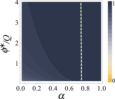
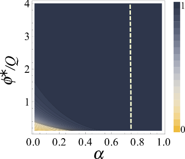
Figure 5: Systemic risk in a system with power law threshold distribution: (left) $\gamma=1.5$, (right) $\gamma=3.0$, for a Bethe lattice with $K=4$, $N=1000$. Cf. also Fig. 4.

The results are to be compared with Fig. 5, where we plot the systemic risk $X$, for Bethe lattices only, for a power law threshold distributions with two different exponents $\gamma$. We remind that the network capacity $Q$ is comparable to the case of the uniform threshold distribution only for $\gamma=3$, Fig. 5 (right) and we also observe a similar dependence of $X$ on the safety margin $(1-\alpha)$ and on the relative initial load $\phi_{\star}/Q$. To be precise, in this case the safety margin plays a less important role, but we find finite cascades also for $\phi_{\star}/Q>0.5$, which was not the case for the uniform threshold distribution.

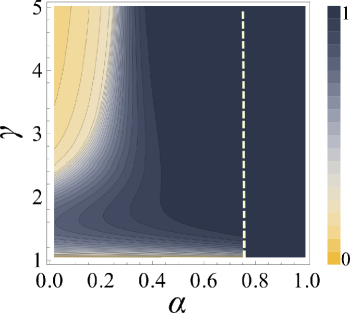
The situation differs for $\gamma=1.5$, as Fig. 5 (left) shows. Here the system seems to be much more vulnerable, indicated by large values of $X$ in all parameter regions. To put this finding into perspective, we remind that for $\gamma<2$ the network capacity is much larger than for $\gamma>2$, i.e. the initial shock also has much higher values as compared to Fig. 5 (right). This explains the severity of the cascades in this case.

The results obtained for these two particular values of $\gamma$ can be generalized to $\gamma\leq 2$ and $\gamma>2$. As a consequence, we may conclude that with a much broader threshold distribution, the system can absorb higher initial shocks (in absolute values), but shocks of a size comparable to the network capacity most likely result in infinite cascades, i.e. total failure.

Figure 6: Systemic risk in a system with power law threshold distribution. The relative initial shock was fixed: $\phi_{\star}/Q=0.2$. $N=1000$, $K=4$. (Left) Bethe lattice, (right) 2D regular lattice. Cf. also Fig. 5.

To better understand the role of the skewness of the threshold distribution and the topology, we fix the relative initial shock $\phi_{\star}/Q=0.2$ and vary $\gamma$ for two different network topologies. Fig. 6 confirms (a) that a Bethe lattice or regular tree structure leads to more severe cascades as compared to a regular network, which is due to the smaller diameter of the network, and (b) that an increasing skewness, i.e. smaller values of $\gamma$ lead to an increasing systemic risk. Remarkably, there is a non-monotonic dependence of $X$ on $\alpha$ and $\gamma$, and the cascade size becomes larger around $\gamma\approx 1.5$. The reason for this is, on the one hand, the system size dependence of the network capacity for $\gamma\leq 2$ and, on the other hand, the larger fragility resulting from a more skewed distribution (i.e. thresholds are closer to $\theta_{\mathrm{min}}$). The first effect is a global one, i.e. larger load is added to the system, the second is a local one, i.e. there are fewer agents that can handle large loads.

3.3 Results for the RIE regime

The previous results have focused on the EEE regime of large external shocks, $\phi_{\star}\sim Q\gg\bar{\theta}$. This means that the initial load is largely responsible for triggering the cascades. Here we focus on the opposite case, the RIE regime, $Q\gg\phi_{\star}\sim\bar{\theta}$, where small fluctuations of an agent’s load lead to the agent’s failure provided that the safety margin of that agent was rather small. The question is then under which conditions this failure leads to a cascade of macroscopic size. Applications of this case include power-grid cascade failures [motter2002cascade, crucitti2004model, CRUCITTI_cascades_power_grid], or failures of server infrastructure [rossi2009].

We now consider $\phi_{\star}=\theta_{i}$ for the failing agent, and we assume that the system is in a critical condition. This means that a single failure among the neighbors of the initially failing agent (i.e. $f(1)\geq 1/K$) is enough to trigger a system-wide cascade. We now define $\phi_{\star}^{c}$ as the load such that $f(1)$ is exactly equal to $1/K$. With these assumptions, we compute the ensemble average $\left\langle X\right\rangle$ of the systemic risk

$$\langle X\rangle=\int_{\phi_{\star}^{c}}d\theta_{i}\,P(\theta_{i}).$$ (38)

The integral runs over the threshold $\theta_{i}\geq\phi_{\star}^{c}$ of all possible agents $i$ which trigger a full cascade. These agents can be regarded as systemically important because their failure induces a systemic collapse.

The quantity $\langle X\rangle$ then represents the frequency at which a randomly chosen agent can trigger the complete failure of the system. In the following we compute $\langle X\rangle$ for the uniform and power-law thresholds distribution.

Uniform threshold distribution

The initial critical load $\phi_{\star}^{c}$ in the RIE regime can be easily computed from Eq. (30), using the condition $f(1)=1/K$:

$$\phi_{\star}^{c}=K(1-\alpha)\left[{2\sigma}/{K}+(\bar{\theta}-\sigma)\right].$$ (39)

Then, the average systemic risk for the uniform distribution $\left\langle X_{u}\right\rangle$ is given by

$$\left\langle X_{u}\right\rangle=\begin{cases}0&\mathrm{if}\quad\bar{\theta}-\sigma>\phi^{c}_{\star}\\ \left[(2\alpha-1)-K(1-\alpha)\right]/2-\bar{\theta}\left[K(1-\alpha)-1\right]/{2\sigma}&\mathrm{if}\quad\bar{\theta}-\sigma\leq\phi^{c}_{\star}\leq\bar{\theta}+\sigma\\ 1&\mathrm{if}\quad\phi^{c}_{\star}>\bar{\theta}+\sigma\end{cases}.$$ (40)

Power-law threshold distribution

In an analogous way we obtain from Eq. (34) with $f(1)=1/K$ the expression for the initial critical load $\phi_{\star}^{c}$ in the case of a power-law threshold distribution:

$$\phi_{\star}^{c}=\theta_{\min}K(1-\alpha)(1-K^{-1})^{-{1}/{\gamma-1}}.$$ (41)

This allows us to calculate the average systemic risk as:

$$\langle X_{p}\rangle=\begin{cases}\frac{1-{K}^{-1}}{\left[K(1-\alpha)\right]^{\gamma-1}}&\text{if}\quad\phi^{c}_{\star}\geq\theta_{\min}\\ 1&\text{otherwise}\end{cases}.$$ (42)

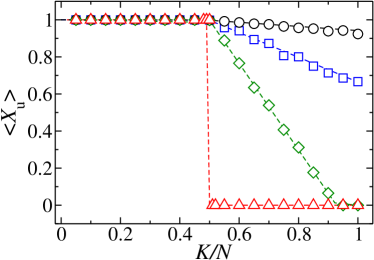
Figure 7: Frequency of “infinite” cascades $\left\langle X\right\rangle$ for the uniform (left) and the power law (right) threshold distribution in the RIE regime. We consider regular random networks of size $N=1000$ with varying $K$; the safety margin of agents is set to $(1-\alpha)=0.002$. Open symbols show simulation results, dashed lines analytic results. Parameters for the uniform distribution: $\bar{\theta}=1$, $\sigma=0$ (triangles), $\sigma=0.3$ (diamonds), $\sigma=0.6$ (squares), and $\sigma=0.9$ (circles). Parameters for the power law distribution: $\gamma=1.1$ (circles), $\gamma=2$ (squares), $\gamma=3$ (diamonds), and $\gamma=4$ (triangles).

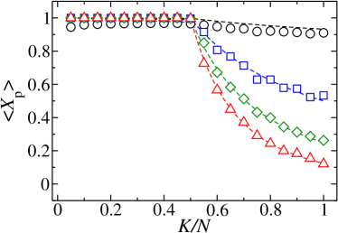
In order to study the role of connectivity in the cascade process, we created random regular networks [construction] with arbitrary values of the average connectivity $K/N$. Fig. 7 shows the average cascade size $\langle X\rangle$ for a rather small safety margin, which is in line with the RIE regime. This means that small fluctuations of the load of a single agent may lead to its failure. Fig. 7 allows to compare the analytical expressions in Eqs. (40), (42) with numerical simulations of the cascade process. The graphs show a sharp transitions from $\left\langle X\right\rangle=1$ to $\left\langle X\right\rangle<1$ at $K/N=1/2$. This results directly from the change in global instability $K(1-\alpha)\leq 1$, at that particular point. On the other hand, when the system is not globally unstable, the results show that only a subset of agents are able to trigger a cascade in the system, their fraction indicated by $\left\langle X\right\rangle$

The left panel of Fig. 7 shows the results for the uniform threshold distribution. For identical agents (left panel, $\sigma=0$), a sharp transition between complete failure ($\left\langle X\right\rangle=1$) and no failure ($\left\langle X\right\rangle=0$) can be observed. This result immediately follows from Eq. (25), in the limiting case $t\to\infty$. For a fixed value $K/N>1/2$, the graphs show that larger values of $\sigma$ exhibit larger frequencies of full cascades, $\langle X\rangle$. This results from Eq. (39) which shows that the critical initial load $\phi^{c}_{\star}$ decreases for increasing heterogeneity; thus, for larger values of $\sigma$ a larger fraction of agents is likely above such a threshold.

The right panel of Fig. 7 shows the results for the power-law threshold distribution. Again, broader distributions, i.e. lower values of $\gamma$, result in a higher probability of complete failures. This is in line with Eq. (41) where, for a fixed $K$, the critical load increases with $\gamma$. At the same time, the threshold distributions become more narrow with larger $\gamma$. Thus, the amount of systemically important agents that are able to trigger a full cascade, is much lower in distributions with large $\gamma$, and thus the average systemic risk decreases.

4 Conclusions

The model proposed in this paper is based on very simple ingredients, to allow for analytical treatment: (i) a regular network, i.e. all agents have the same number of neighbors, $K$, (ii) a constant safety margin $(1-\alpha)$, the same for all agents, which defines a fixed relation between the load $\phi_{r}$ an agent can possibly carry and the threshold $\theta_{r}$ at which it fails, (iii) an initial condition that only one randomly chosen agent $i$ fails when facing a load $\phi_{\star}$, (iv) a redistribution of the load of the failing agent to its $K$ neighbors.

The variability of the model comes from two assumptions: (v) the threshold distribution $P(\theta)$ which was chosen as a delta distribution, a uniform distribution, or a power law distribution, (vi) the severity of the initial shock, which was either of the order of the network capacity $Q$, i.e. much larger than the average threshold, or much smaller than the network capacity, i.e. of the order of the average threshold. The latter allowed us to distinguish between two important regimes: (a) EEE regime, where an extreme external event was large enough to cause the failure of many agents, (b) RIE regime, where small random internal events may result in the failure of a single agent. In both cases, this initial failure may have triggered a cascade of failures in the neighboring agents.

For both regimes, we are interested in the following question: what is the possible size of a failure cascade, $X(t)$, measured as the total number of failed agents compared to the system size $N$, at a given time $t$. Will this be an “infinite” ($X\to 1$) or a “finite” ($X<1$) cascade and, in the latter case, at what time will it stop: at a time $t^{\circ}$ where the cascade has already reached all agents but did not cause all of them to fail, or at a time $t^{\star}$ before it has passed the entire system. We regard $X$ as a measure of systemic risk.

For both regimes, we are able to derive analytical results to answer these questions. These results allow us to draw conclusions about the conditions that lead a smaller systemic risk. In the following we summarize our finding:

(1) We derive a global stability condition $K(1-\alpha)\geq 1$ that has to be met in order to allow for finite cascades, in principle. The larger the number of neighboring agents, $K$, or the larger the safety margin, $(1-\alpha)$, the more likely this condition is met. This allows for an interesting discussion because of the possible trade-off between the two ingredients. In most cases, the safety margin is given by the technical constitution of an agent, e.g. in power grids or routing servers. $K$, on the other hand, refers to the network topology but not to internal properties of agents. Hence, systemic risk can be reduced by increasing the network density - at least up to a certain point [Battiston2009a]. It should be noted that we have assumed the initial failure of only one agent, here. If it is, however, more costly to improve the network connectivity than increasing the safety margin of the agents, the latter can serve the same purpose, namely reducing systemic risk.

(2) In a system of thousands of agents, the network capacity, $Q$, which is the total load the system can carry a priori, is also quite big. One would not easily assume that an initial shock $\phi_{\star}$ is of the same magnitude as $Q$ as in the EEE regime. Hence such big shocks are extreme external events to the system. The interesting finding in this paper is that even such extreme events may not lead to an “infinite” cascade, i.e. to a total collapse of the system. Instead, provided that the global stability condition is met, we find a broad range of system parameters where such cascades stop at finite time, affecting only part of the system. We have shown that systemic risk resulting from extreme shocks can be reduced (a) by a regular lattice structure (as opposed to e.g. a regular tree structure), (b) by a broad threshold distribution. In the latter case, we found finite cascades, i.e. $X<1$, even if the initial shock was 2-4 times larger than the total network capacity, which can be regarded as a sign of real robustness. Comparing the power-law threshold distributions of $\gamma=1.5$ and $\gamma=3$, we found that, in absolute measures of the shock, the broader distribution lead to the more robust systems. In relative measures, however, this result inverts, simply because a broader distribution also results for a larger network capacity, and hence for larger initial shocks, while the relative measure remains the same.

(3) Investigating the RIE regime where the initial shock was of the order of the threshold of an average agent, i.e. much smaller than the total network capacity, a systemic failure can occur only if (a) the the initial shock is larger or equal to the threshold of the initially failing agent, and (b) the redistribution of load is large enough. Hence, dependent on the threshold distribution we can calculate this failure probability. Even in the global stability regime, we find “infinite” cascades, but the probability of their occurrence depends on the probability that randomly chosen agent fails initially. The broader the threshold distribution, the more likely this condition is met, i.e. the frequency of observing “infinite” cascades increases with the heterogeneity.

(4) The initial question: “How big is too big”, from this perspective, can be answered as follows: Initial shocks, even if they exceed the capacity of the whole system (not just the capacity of a single agent), are probably not the problem. Of course, there are parameter regimes that lead to complete collapse ($X\to 1$). At the same time, we see that a change of $\phi_{\star}$ of 10 or even 50 percent does not change the systemic risk very much. Of much larger influence are system parameters related to the network topology, the safety margin, and the threshold distribution. As it was also found in other papers [Lorenz2009b], an optimal heterogeneity in the agent’s threshold can reduce systemic risk considerably. In addition to that we find that an change of the safety margin by 10 or 50 percent generates a much larger impact on systemic risk than a comparable change in the external shock. So, when seeking for protection against systemic risk the focus should be (a) on those parameters that influence the global stability, i.e. $K(1-\alpha)$ (see above), and (b) on the optimal heterogeneity in the threshold distribution.