The Milky Way’s circular velocity curve between and from APOGEE data
Abstract
We measure the Milky Way’s rotation curve over the Galactocentric range from the first year of data from the Apache Point Observatory Galactic Evolution Experiment (APOGEE). We model the line-of-sight velocities of 3,365 stars in fourteen fields with between out to distances of using an axisymmetric kinematical model that includes a correction for the asymmetric drift of the warm tracer population (). We determine the local value of the circular velocity to be and find that the rotation curve is approximately flat with a local derivative between and . We also measure the Sun’s position and velocity in the Galactocentric rest frame, finding the distance to the Galactic center to be , radial velocity , and rotational velocity , in good agreement with local measurements of the Sun’s radial velocity and with the observed proper motion of Sgr A∗. We investigate various systematic uncertainties and find that these are limited to offsets at the percent level, in . Marginalizing over all the systematics that we consider, we find that at confidence. We find an offset between the Sun’s rotational velocity and the local circular velocity of , which is larger than the locally-measured solar motion of . This larger offset reconciles our value for with recent claims that . Combining our results with other data, we find that the Milky Way’s dark-halo mass within the virial radius is .
Subject headings:
Galaxy: disk — Galaxy: fundamental parameters — Galaxy: general — Galaxy: kinematics and dynamics — Galaxy: structure — stars: kinematics1. Introduction
The Milky Way’s inner rotation curve , and in particular its value at the Sun’s Galactocentric radius , is crucial for our understanding of many Galactic and extra-galactic observations. It provides an important constraint on mass models for the Milky Way and the question of whether the Galactic disk is maximal. The shape of the rotation curve is an important ingredient for realistic models of the disk’s formation and evolution. The circular velocity at the Sun, which is located approximately disk scale lengths from the Galactic center (Bovy et al., 2012b), is also important for placing the Milky Way in a cosmological context, for example, when asking whether the Milky Way follows the Tully-Fisher relation (e.g., Klypin, Zhao, & Somerville, 2002; Flynn et al., 2006; Hammer et al., 2007). is often considered to be an important parameter for dark-matter direct-detection experiments and for correcting the motion of extra-galactic objects for the motion of the Sun, although we seek to dispel these notions below ( 5.3).
Traditionally, the local circular velocity has been obtained by measuring the Sun’s motion with respect to an object that is assumed to be at rest with respect to the Galaxy. The most robust of those measurements is that derived from the observed proper motion of Sgr A∗ (Reid & Brunthaler, 2004), even though this requires an estimate of . An alternative method that does not require knowledge of consists of measuring the Sun’s reflex motion using a stellar tidal stream with orbital pole near (Majewski et al., 2006). Similar measurements using samples of halo stars (Sirko et al., 2004), or the globular cluster system (Woltjer, 1975), may be contaminated by the residual, presumably prograde, motion of these populations and, thus, only provide a lower limit. As discussed in detail in 5.3, such measurements intrinsically measure the Sun’s rotational velocity, , rather than the circular velocity. To arrive at , these measurements depend on a highly uncertain correction for the Sun’s motion with respect to . The measurement of by observing the extreme line-of-sight velocity of HI emission toward Galactic longitudes in principle also directly measures (Knapp et al., 1979), although the HI density drops too steeply with radius for to be directly observed, and more intricate modeling is necessary to turn the HI emission toward into a constraint on .
Other measurements of have in the past been limited to measurements of the Oort constants, due to a lack of data at large distances from the Sun (e.g., Feast & Whitelock, 1997). Recently, new estimates have been obtained from the kinematics of masers in the Galactic disk (Reid et al., 2009; Bovy et al., 2009a; McMillan & Binney, 2010), and from fitting an orbit to the cold stellar stream GD-1 (Koposov et al., 2010). However, until now, no consensus has been reached as to whether lies near the IAU-recommended value of (Kerr & Lynden-Bell, 1986), or whether it needs to be revised upward to around (e.g., Ghez et al., 2008; Reid et al., 2009; Bovy et al., 2009a; Schönrich, 2012).
Most of the information relating to the shape of the rotation curve is based upon the observed kinematics of the HI emission, either through the tangent-point method at and (van de Hulst et al., 1954; Gunn et al., 1979; Levine et al., 2008), or through the observed thickness of the HI layer at (Merrifield, 1992). Such measurements are purely geometrical and, in particular, cannot constrain the component of Galactic rotation that has a uniform angular speed. This also holds for measurements of based on the line-of-sight velocities of open clusters (e.g., Frinchaboy, 2008). The best constraints on the local slope of the circular-velocity curve therefore also come from measurements of the Oort constants (e.g., Feast & Whitelock, 1997), although the HI observations are crucial to measuring the rotation curve over the full radial range of the disk.
In this paper we present the first measurement of the Milky Way’s circular velocity curve using kinematically-warm stellar tracers out to heliocentric distances of , from the Sloan Digital Sky Survey III’s Apache Point Observatory Galactic Evolution Experiment (SDSS-III/APOGEE; Eisenstein et al. 2011; S. R. Majewski, et al. 2012, in preparation). APOGEE is a high-resolution spectroscopic survey covering all of the major components of the Galaxy that—crucially—operates in the near-infrared, which allows stars to be observed to large distances in the dust-obscured regions of the inner Milky Way disk. While warm stellar-disk tracers do not on average rotate at the circular velocity like the HI emission discussed above, their offset from —the so-called asymmetric drift (Strömberg, 1946)—is a dynamical effect that can be calculated from their observed velocity dispersion. Because our measurement relies on a dynamical effect, we are sensitive to in the sense of the radial-force component at , rather than to , although the large range in of our sample allows us to independently measure . Additional benefits of using the intermediate-age to old stellar population to trace the dynamics of the disk are that these populations are much less sensitive to non-axisymmetric streaming motions than cold gas, and that the large asymmetric drift can be used to constrain the component of Galactic rotation that possesses a uniform angular speed.
Using a data set of 3,365 stars at along 14 lines of sight covering , we find that the Milky Way’s rotation curve is approximately flat over , with . A value of is ruled out at confidence by our data. Our measurement of agrees with the observed proper motion of Sgr A∗, but the Sun’s offset from is larger than the locally-measured value (Schönrich et al., 2010) by .
The outline of this paper is as follows. In 2, we describe the APOGEE data set. The methodology employed to model the observed kinematics of the kinematically-warm tracer population is presented in 3. We discuss our results in 4, including a detailed discussion of potential systematics in 4.2. The influence of non-axisymmetric streaming motions on our data is assessed in 5.1. We compare our new measurement of with previous determinations in 5.2. In 5.3, we discuss the implications of our measurement of the Sun’s offset from circular motion and, in 5.4, we estimate the mass of the Milky Way implied by our data, as well as other recent data. We conclude in 6. Appendix A describes how photometric distances for the stars in our sample are estimated. In Appendix B we discuss extensive mock-data tests used to test our methodology and to determine the data’s sensitivity to . In what follows we sometimes refer to the circular velocity at the Sun’s location by the shorthand notation .
2. APOGEE Data
The SDSS-III/APOGEE is a near-infrared (NIR; -band; 1.51 to 1.70 m), high-resolution (R 22,500), spectroscopic survey, targeting primarily red giants in all Galactic environments, with emphasis on the disk and the bulge. The APOGEE instrument (Wilson et al. 2010, J. Wilson et al. 2012, in preparation) consists of a spectrograph with 300 fibers that reaches a signal-to-noise ratio of per pixel (at about Nyquist sampling) at in three one-hour visits during bright time on the 2.5-meter Sloan telescope, at the Apache Point Observatory in Sunspot, NM (Gunn et al., 2006). A detailed account of the target selection and data reduction pipeline is given in G. Zasowski et al. 2012 (in preparation) and D. Nidever et al. 2012 (in preparation), respectively. Here we summarize the, for our purposes, most important aspects of the target selection and data reduction.
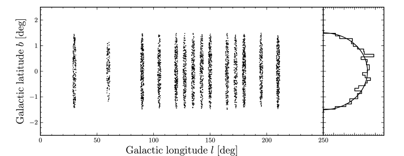
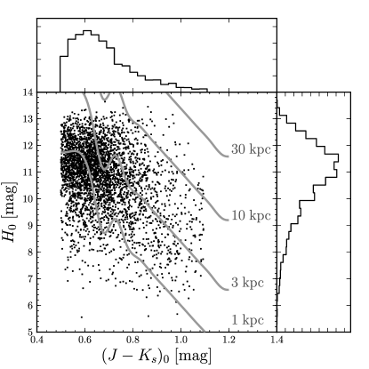
Our analysis is based on data from APOGEE’s first year of regular survey operations (09-11-2011 to 05-07-2012). We use data from fields centered on ; APOGEE fields have a radius of 1.5∘. By only selecting fields with we avoid the bulge region. We resolve multiple visits to the same field by choosing the highest signal-to-noise ratio measurement of the Doppler shift, rather than combining the multiple epochs, because the typical uncertainty in the line-of-sight velocity is well below 1 km s-1. Only primary survey targets are selected, excluding targets flagged as possible cluster members and stars observed as part of any of various special programs. We exclude stars with , as these are problematic for the isochrone model we adopt to marginalize over their distances (see Appendix A). The resulting sample has 3,365 stars in 14 different fields with . The distribution of the data in extinction-corrected color and magnitude is shown in Figure 1 and the distribution of the stars on the sky is shown in Figure 2. The properties of the sample in the various fields are given in Table 2.
Spectroscopic targets are selected from the 2MASS point-source catalog (Skrutskie et al., 2006), with the following quality restrictions applied: photometric uncertainties less than 0.1 mag in , , and ; quality flag ‘A’ or ‘B’ in ; nearest neighbor more than away; confusion flag ‘0’ for ; galaxy contamination flag ‘0’; read flag ‘1’ or ‘2’ for ; extkey equal to . The extinction corrections for targets in the Galactic mid-plane use mid-IR photometry from either WISE (Wright et al., 2010) or Spitzer-IRAC GLIMPSE-I (Churchwell et al., 2009); therefore, both mid-IR detections and mid-IR photometric uncertainties less than 0.1 mag are required111The first version of the APOGEE target selection did not consistently insist on the availability of extinction corrections, such that a small number of mid-plane targets do not have extinction estimates. We have removed 17 stars without extinction estimates from the sample.. APOGEE’s magnitude range——is within the completeness limits for both the IRAC and WISE surveys. Photometry for all targets is extinction-corrected using the Rayleigh Jeans Color Excess method (RJCE; Majewski et al., 2011), which provides extinction values with typical random uncertainties mag for individual stars using a combination of near- and mid-IR photometry. Variations in the adopted extinction law among different lines of sight can lead to differences of up to 7% (Zasowski et al., 2009).
| Field location | Stars | median | |||
|---|---|---|---|---|---|
| [degrees] | |||||
| 230 | 108 | 33 | 89 | 0.8 | |
| 141 | 50 | 33 | 58 | 0.6 | |
| 310 | 178 | 46 | 86 | 0.4 | |
| 222 | 222 | 0 | 0 | 0.2 | |
| 289 | 157 | 84 | 48 | 0.3 | |
| 228 | 228 | 0 | 0 | 0.3 | |
| 229 | 229 | 0 | 0 | 0.3 | |
| 227 | 227 | 0 | 0 | 0.6 | |
| 279 | 150 | 87 | 42 | 0.3 | |
| 225 | 225 | 0 | 0 | 0.1 | |
| 199 | 199 | 0 | 0 | 0.3 | |
| 314 | 174 | 90 | 50 | 0.2 | |
| 227 | 227 | 0 | 0 | 0.2 | |
| 315 | 173 | 91 | 51 | 0.2 |
The color range that we select, , includes the red clump (( to 0.7) and the red giant branch, for all metallicities. Dwarf contamination is most severe at (, with most redder dwarfs being faint M and brown dwarfs. Most APOGEE observations consist of three or more individual “visits”, with only three visits for stars with 7 , and six visits for . About 10% of our sample consists of even more visits for stars with . The APOGEE sampling is random in color, and a combination of random and systematic in apparent magnitude (selecting every -th star in a magnitude-ordered list for each field); details of the selection function are unimportant for our purposes and it suffices to note that the spectroscopic sample is a representative sample of the underlying (non-extinction-corrected) magnitude distribution. At , dwarf contamination in the APOGEE fields is expected to be less than 10% based on population-synthesis models (Girardi et al., 2005) in the APOGEE fields (L. Girardi, 2012, in preparation). Models predict that this contamination increases to about 20% at . We explicitly include dwarf contamination as a free parameter in the analysis below.
Line-of-sight velocities are determined for each individual visit by cross-correlating against a set of 100 synthetic template spectra that sparsely cover the stellar-parameter range K K in effective temperature, , in metallicity, , and in surface gravity, (see D. Nidever et al. 2012, in preparation, for details on the exact procedure). The distribution of rms scatter in the measured line-of-sight velocity for stars with multiple observations peaks around . Tests of field-to-field variations indicate that the zero point of the velocity scale is stable at the level. A preliminary comparison between the APOGEE-measured and literature line-of-sight velocity of 53 stars in M3, M13, and M15 shows that the APOGEE zeropoint accuracy is (see D. Nidever et al., 2012, in preparation for full details). In what follows we ignore the uncertainties on the line-of-sight velocities entirely (that is, we assume that they are zero), because the uncertainties are much smaller than any velocity difference that we could hope to measure with our sample of stars having a typical dispersion of .
Repeated visits to the same star will eventually allow binary stars to be flagged as such based on the variability of their line-of-sight velocities. However, currently multiple visits are not available for all 14 APOGEE fields that we employ here, and removing fields without multiple visits would significantly reduce the longitudinal coverage of our sample. Using the stars in our sample that have multiple visits, we find that of stars show velocity variability at the to level—the level at which they could be confused with the dispersion of a disk population. Binary contamination would spuriously increase the inferred velocity dispersion and therefore likely decrease the inferred circular velocity, due to the dispersion-dependence of the asymmetric-drift correction used below. However, as discussed below, the asymmetric drift for our sample is at , such that the effect of binary contamination on the velocity dispersion is . Therefore, we do not remove binaries from our sample, but we discuss the results obtained when removing them in 4.2.
Stellar parameters and elemental abundances are determined by the APOGEE Stellar Parameters and Chemical Abundances Pipeline (ASPCAP; A. E. García Pérez et al., 2013, in preparation). After determining the spectral type, each star’s microturbulence, , , , , , and are determined through minimization of the difference between the observed and synthetic spectra derived from ATLAS9 model-atmosphere grids (Kurucz 1979 and more recent updates). We only use in our analysis below, and in particular, we do not make use of for the purpose of selecting giants, because the measurement of has not been finalized yet within ASPCAP. Preliminary comparisons with standard stars and globular clusters indicate that the metallicities are currently accurate, to a precision of at . All but of the disk stars in our sample described below have higher metallicities than this, and all but have .
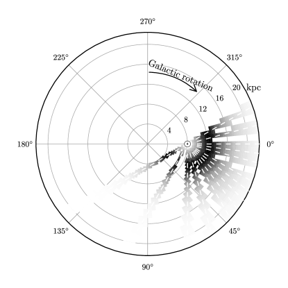
Because many stars in our sample are on the red giant branch, and hence do not follow narrow magnitude-color relations like dwarfs and red clump stars, estimating precise distances to these stars is difficult. In what follows, we avoid estimating distances to the individual stars in our sample by marginalizing a kinematical model over the distance to the star. This marginalization is performed by integrating over the full photometric-distance probability distribution function (PDF) for each individual star, obtained from models for the stellar isochrones and initial mass function (IMF) of the giant stars in the sample, as well as a prior that the stars are in an exponential disk with a scale length of 3 kpc (Bovy et al., 2012c). This technique is discussed in detail in Appendix A. For dwarf stars, we assume that they are close enough that their distances are irrelevant for their kinematics. As such, we cannot show the spatial distribution of the stars in our sample. As an alternative, we show in Figure 3 the sum of all of the photometric distance distributions for stars in our sample (assuming that they are all giants).
3. Methodology
3.1. General Considerations
Our approach to determining the Milky Way’s rotation curve from the APOGEE data is to fit a kinematical, axisymmetric model to the observed line-of-sight velocities. In its most basic form, such a kinematical model consists of (a) a model for the rotation curve, (b) a model for the distribution of peculiar velocities with respect to circular motion as a function of Galactocentric radius, and (c) a set of parameters describing the transformation of positions and velocities from the heliocentric to the Galactocentric frame. These latter parameters are the distance from the Sun to the Galactic center, and the Sun’s velocity with respect to the (dynamical) center of the Galaxy. We will ignore the small projection effects that arise at non-zero Galactic latitude and the vertical dependence of , since these are all at the sub-km s-1 level for and distances (e.g., Bovy & Tremaine, 2012). Therefore, we are only concerned with motions in the plane of the Galactic disk, and we ignore vertical motions.
The kinematical model provides the probability distribution of line-of-sight velocities as a function of position (Galactocentric radius and azimuth , or distance and Galactic longitude ), after marginalizing over the component of the velocity tangential to the line of sight. This requires knowing the distance, which is only weakly constrained for giants (see Appendix A). Therefore, we additionally marginalize the kinematical model over the distance to each star, to obtain the probability of the observed line-of-sight velocity of a star, given its position , photometry (), the iron abundance (taken as representative of the overall metallicity of the star), the kinematical model (represented by the circular-velocity curve and the distribution of peculiar velocities, ), and the coordinate-transformation parameters and (where we label this parameter as “gal” to emphasize that this is the full velocity with respect to the center of the Galaxy, not just the Sun’s motion with respect to the local circular velocity):
| (1) |
The first factor within the integral is produced by marginalizing the kinematical model over the velocity component tangential to the line of sight at a given position. The second factor is given by the photometric-distance PDF, discussed in Appendix A; we include ‘iso’ in the prior information to emphasize that we use an isochrone and IMF model to obtain the photometric-distance PDFs. We also marginalize over whether a star is a giant or a dwarf star, which changes the photometric-distance PDF; the dwarf contamination probability is a single free parameter in our model. Equation (1) is the likelihood for a single star, and the total likelihood for the sample is calculated by multiplying together the individual likelihoods for all the 3,365 data points. This total likelihood is what we optimize to fit models to the data.
We can also calculate the distribution of line-of-sight velocities for individual fields, which we will use later to show comparisons between the best-fit model and the data. For the distribution of of a field centered at (,) we obtain
| (2) |
where is taken directly from the field’s data (that is, we sum over the data (,,,,)).
3.2. Kinematical Model
We now describe in detail the full model that is fit to the data. Our fiducial model for the distribution of velocities in the Galactocentric rest frame is that it is a single biaxial Gaussian, with a mean radial velocity of zero because of the assumption of axisymmetry, and a mean rotational velocity given by the local circular velocity , adjusted for the local asymmetric drift , which is a function of the velocity dispersion, , and the radial and radial-velocity dispersion scale lengths of the population ( and , respectively, see below). The only free parameters of the distribution of peculiar velocities are therefore the radial and rotational velocity dispersions, as the mixed radial–azimuthal moment vanishes, again because of the assumption of axisymmetry. The mixed moment, or equivalently the vertex deviation, in the solar neighborhood does not vanish for the warm disk population (Dehnen & Binney, 1998), but this seems likely to result from the presence of moving groups, and not from the smooth underlying distribution having a strong non-zero vertex deviation (Bovy et al., 2009b).
Assuming that the distribution of velocities in the Galactocentric cylindrical frame is Gaussian allows us to analytically marginalize the velocity distribution over the velocity component tangential to the line of sight. The resulting one-dimensional distribution is itself Gaussian, with mean and variance , where is the ratio of the rotational and radial velocity variances . The Galactocentric line-of-sight velocity for a star is calculated from its heliocentric line-of-sight velocity
| (3) |
where we have written the Sun’s velocity in terms of its angular velocity . This angular velocity is expected to be close to the observed proper motion of Sgr A∗ in the plane of the Galaxy (30.24 km s-1 kpc-1; Reid & Brunthaler 2004), but we leave it as a free parameter, in addition to .
The asymmetric drift in the plane of the Galaxy of a population of stars is given by (e.g., Binney & Tremaine, 2008)
| (4) |
assuming that the radial–vertical velocity moment in the Galactic plane, for symmetry reasons. For an exponential-disk tracer population (stellar tracer density ) with an exponentially declining radial-velocity dispersion (), this formula becomes
| (5) |
The main unknown in this relation is and its dependence on . In the fit below, we assume a constant with for calculating the model’s Gaussian line-of-sight velocity dispersion (see above), but to model the asymmetric drift more realistically, we use an coming from an axisymmetric equilibrium model for the distribution function in a disk with a constant circular velocity with radius. For this distribution function, we use a Dehnen distribution function (Dehnen, 1999) given by
| (6) |
where , , and are the radius, angular momentum, and angular velocity, respectively, of the circular orbit with energy . Using the procedure given in 3.2 of Dehnen (1999), we choose the and functions such that they reproduce a disk with exponential surface density and velocity-dispersion profiles to an accuracy of a fraction of a percent at all radii.
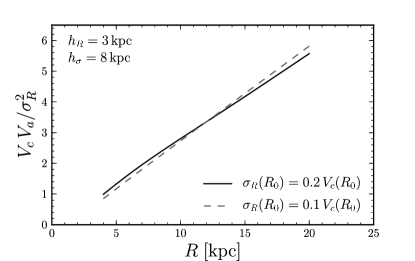
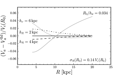
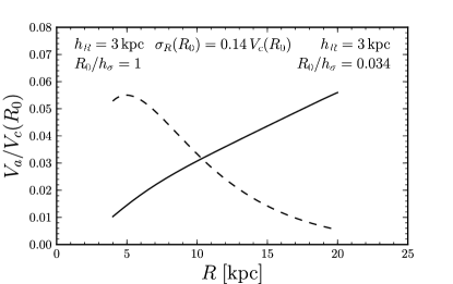
The asymmetric drift for the Dehnen distribution function (DF) for a population with km s-1 is shown in Figure 4 for , . The same is shown for a population with km s-1, and the difference, normalized for the difference in between them, is small. For different values of and we correct this function using Equation (5). As different values for and lead to a different , this approach is slightly incorrect, but tests show that the difference in is for reasonable values of and . As the asymmetric drift is typically km s-1 for our sample, this leads to changes km s-1, which we can ignore. Similarly, differences in for our sample from this model are typically , also leading to changes km s-1, such that our assumption of a constant does not strongly bias the value of the inferred circular velocity. In the exponential-disk model, the asymmetric drift for our sample is km s-1 at all radii, even in the innermost disk (Freeman, 1987).
The middle panel of Figure 4—now for , the best-fit value below—shows the difference in asymmetric drift for different values of and ; the main difference is at small . This figure shows that the dependence of the asymmetric drift correction on and at is mostly —as it is unlikely that the scale length is as small as 2 kpc for this sample of stars (Bovy et al., 2012c), or that the radial-velocity dispersion scale length is much shorter than 8 kpc—which is the same as the statistical uncertainty on the circular velocity that we infer below. Therefore, the systematic uncertainty due to the scale length of the population of stars is km s-1 at , and likely km s-1. We could directly measure the scale length of our sample, but as this requires a detailed understanding of the dust distribution in the plane of the Galaxy, and as it does not contribute greatly to the error budget of our measurement, we do not attempt it here.
Our best-fit model below has a radial velocity dispersion that is approximately flat over the range in considered here. In this case, the asymmetric-drift correction increases with , as is clear from Equation (5), and the difference between this dispersion profile and that considered above is shown in the middle panel of Figure 4. The bottom panel of Figure 4 shows the actual asymmetric-drift correction applied in our best-fit model below. It is clear that this correction is small ( at ); hence it does not drive our inferred value for below. The bottom panel of Figure 4 also illustrates that, if the dispersion scale length were smaller than that in our best-fit model below, then the circular velocity curve would drop more steeply than what we infer below.
In addition to the kinematical model discussed so far, we include an outlier model that consists of a Gaussian with a width of , centered on a mean value that is a free parameter in the model. This outlier model exists primarily to deal with data-processing outliers, stars with a color and magnitude that places them beyond the disk, and close binaries with large velocity amplitudes (as we do not currently have a sufficient number of APOGEE epochs for each star to confidently remove these from the sample). In all of the fits below, the outlier fraction is , thus it does not influence our fits.
3.3. Dwarf Contamination
The dwarf contribution to the likelihood in Equation (1) could in principle be treated in the same way as the giant contribution, by integrating over the obtained from a similar isochrone and IMF model as for the giants. However, this is problematic, because the main sequence is much narrower than the giant branch, such that this integral is dominated by a narrow range of distances. As all of the dwarfs in our sample are faint main-sequence stars, they are expected to all be within a few 100 pc from the Sun, and thus be relatively unaffected by the radial and azimuthal gradients in velocity distribution that we model for the giant stars. Our approach is therefore to replace the integration over distance with a single evaluation at zero distance from the Sun for the dwarf part of the likelihood. The dwarf stars are otherwise modeled using the same distribution of peculiar velocities as the giant stars, i.e., we assume that they are drawn from a similar population. The dwarf contamination in our best-fit model below is , and is similar for other fits considered below. This is close to the value expected from stellar-population-synthesis models (see 2).
3.4. Mock Data Tests
The procedure described above makes non-trivial approximations to an ideal axisymmetric fit to the data. The most important of these is that, although we include the asymmetric drift as part of our model, we do not include the deviations from a Gaussian rotational-velocity distribution that are expected for a warm population of stars (with the same physical origin as the asymmetric drift). In addition to this assumption, we make small approximations to the full asymmetric drift expression in Equation (4). These simplifications are expected to have small effects on our analysis: The skew of the rotational-velocity distribution is only fully visible near the tangent point where the line-of-sight velocity is equal to the rotational velocity, but our sample covers a large range of distances for each line of sight, and 85% of our sample lies at , where there is no tangent point. As such, most stars are drawn from a distribution that is close to Gaussian.
To investigate these simplifications, we conduct a series of mock data tests. In these tests, we sample line-of-sight velocities from the best-fit flat-rotation-curve model below, except that we use the full Dehnen DF of Equation (6)—uncorrected, such that it does not quite reproduce the assumed exponential disk—rather than the Gaussian approximation used in the fit (we ignore the best-fit as the Dehnen DF has built-in). We then fit these mock data using the approximate methodology.
These mock data tests are described in detail in Appendix B. The results from these tests show that the approximations made in the analysis do not produce any significant bias in the fitted parameters. Fits with non-flat rotation curves to the mock data samples indicate that we can reliably determine the shape of the rotation curve between . The uncertainties in the fitted parameters for the mock data are approximately the same as those for the real data (see below), which indicates that the uncertainties in the Galactic parameters derived below for the real data are correct.
3.5. Parameter Sensitivity
We briefly discuss here how our data are sensitive to the parameters of the model. The mean heliocentric line-of-sight velocity at a position is given by (see Equation (3))
| (7) |
where . We have treated the position and velocity of the Sun as free parameters, without imposing any prior on , and without assuming that the solar rotational velocity is given by the local circular velocity corrected for the (previously measured) velocity of the Sun with respect to the local standard of rest (LSR). We can determine the full space motion of the Sun from our sample, because the longitudinal dependence of the correction for the solar motion of the line-of-sight velocity of a star at is sinusoidal (), while the dependence on the rotational velocity at the position of the star varies differently for the to sample of APOGEE stars (). Mock data tests in Appendix B show that our sample spans a sufficiently wide range in Galactic longitude and distance to disentangle these two effects, and measure the solar Galactocentric motion. Because we know the Sun’s rotational frequency from assuming that the radio source Sgr A∗ at the Galactic center is at rest with respect to the disk, we have an independent check on our inferred value for the solar motion (but we do not use the measured proper motion of Sgr A∗ as a prior on the solar motion).
We can then turn a measurement of into a measurement of by correcting for the asymmetric drift, , using Equation (5). This transformation requires a measurement, foremost, of the radial-velocity dispersion, . We can measure almost directly using the line of sight. By modeling as an exponential and assuming a constant , we can measure from the line-of-sight-velocity dispersion at each . The only subtlety here is that, in the first quadrant (), we typically sample positions where is close to , while in the second and third quadrants (), is mainly composed of . We can then use the measurement of to correct for and derive .
The fact that our data sample is composed of the intermediate-age to old disk population is crucial for our ability to measure the full shape of the rotation curve. Traditional tangent-point analyses of the HI emission at , or the measurement of at using the thickness of the HI layer, are insensitive to solid-body (uniform angular speed) contributions to the rotation curve, because these do not give rise to line-of-sight velocities for circular orbits. Formally, the HI velocities are invariant under the transformation . However, this is not the case for a warm tracer population, as, for example, the mean rotational velocity transforms as
| (8) |
where . Thus, the addition of to changes by , and gives rise to a few changes in , which we can detect with our data. Equation (8) clearly shows that a warmer population, i.e., a population with a larger asymmetric drift, is more sensitive to the local slope of the rotation curve than a colder population.
4. Results
4.1. Basic Models
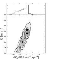
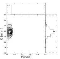
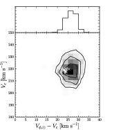
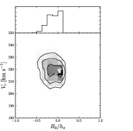
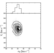
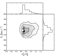
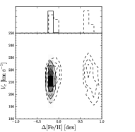
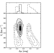
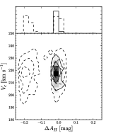
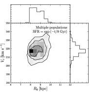
In this section, we discuss the results from fitting the basic kinematical model of a single population with exponential and profiles to the APOGEE disk mid-plane data from 2. These are the main results of this paper. In a subsequent section, we discuss the effects of various systematics on these basic model fits, but we find in the end that they do not significantly bias the results for the Galactic parameters in this section.
| Parameter | Flat rotation curve | Power-law | ||
|---|---|---|---|---|
| … | ||||
| … | ||||
| … | ||||
Note. — Maximum-likelihood best-fit results; uncertainties are given as 68% intervals of the marginalized PDF for each parameter. The first block of parameters are the basic Galactic parameters: circular velocity at the Sun’s location, the derivative of the circular-velocity curve with , and various other representations of these two basic parameters: the Oort parameters and , the rotational frequency at the Sun’s location, and the combination that is relevant in the determination of the local dark matter density using the cylindrical Poisson equation. The second block of parameters describe the Sun’s phase-space position in the Galaxy: distance to the Galactic center, the Sun’s radial velocity (away from the Galactic center), the Sun’s Galactocentric rotational velocity , and the Sun’s peculiar velocity with respect to local Galactic rotation . We also give the proper motion of Sgr A∗ derived from the previous parameters assuming that Sgr A∗ is at rest with respect to the disk. The final block of parameters describe the tracer population sampled by APOGEE: radial velocity dispersion at , the radial scale length of the radial velocity dispersion (given as ), and the ratio of the tangential to the radial velocity variance .
The results from fitting a flat rotation curve to the APOGEE data are given in the left column of Table 4. The right column of this table gives the results when fitting a power-law model for the rotation curve . The best-fit power-law index in this case is approximately zero, such that both models for the rotation curve yield similar best-fit values for all parameters. The only significant difference between the two models for the rotation curve is the uncertainty interval for , which extends to lower values of in the case of the power-law fit, although the upper limit on stays approximately the same. We find that is tightly constrained in the flat rotation-curve model: (68% confidence). When fitting a power law we find , with a strong correlation between the power-law index (or, equivalently, the local derivative of the circular velocity with respect to ) and . Other parameters do not exhibit any strong correlation with (see discussion below).
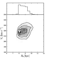
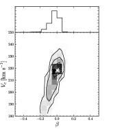
When fitting a power-law model for the rotation curve, the local slope of the rotation curve is constrained to be (68% confidence), with a best-fit value near the upper end of that range, . When fitting a linear model for the circular velocity the constraints are similar, and we do not discuss them further; the top, middle panels of Figure 5 show the joint PDF for and (for the power-law fit) and (for the linear fit). In Table 4, we also give the Oort constants and corresponding to the and inferred directly for our sample (for the case of a flat rotation curve, and are equal in magnitude and opposite in sign, by definition). We also present the combination , which is the correction term that must be added to the local dark-matter density to account for a non-flat rotation curve, when the local dark-matter density is inferred from local vertical kinematics using the cylindrical Poisson equation (e.g., Bovy & Tremaine, 2012). It is clear that we constrain this correction term to be smaller than a fraction of the local dark-matter density: , compared to a local dark-matter density of (Bovy & Tremaine, 2012). Thus, the correction for the non-flatness of the rotation curve for our best-fit parameters is approximately zero, and at 68% confidence it lies between and . We also give the rotational frequency at the Sun’s location.
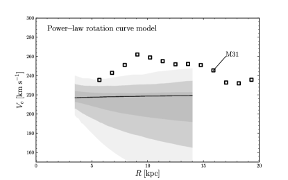
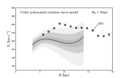
Using a power-law rotation-curve model, we estimate the uncertainty in the rotation curve by evaluating the range of at each for 10,000 samples from the PDF shown in Figure 5. Thus, every sample has a power-law rotation curve, but the range at each does not have to follow a power law itself. This exercise shows whether, in the power-law model, the value of is well-constrained or not for each ; The result is shown in the left panel of Figure 6. The same is shown in the right panel of that figure for a fit assuming a cubic-polynomial model for the rotation curve. However, in the latter model we have imposed a prior that , as a large number of samples from the PDF have , which we assume to be implausible from prior data (e.g., Ghez et al., 2008; Gillessen et al., 2009). We emphasize that we do not include such a prior in any other part of the analysis presented here. We see that the rotation curve is best constrained at small radii (), and that it is largely consistent with being close to flat over the full range of Galactocentric radii considered here.
We also determine the full planar phase-space position of the Sun in the Galactocentric reference frame. The current APOGEE data are relatively insensitive to the value of . The 68% interval for for both the flat-rotation-curve and power-law fits is about , which is similar to that found for the mock data in Appendix B. The best-fit value is at the lower end of this range: when assuming a flat rotation curve, for the power-law rotation-curve fit. The fully marginalized PDF for in the top, left panel of Figure 5 is almost entirely flat between .
The Galactocentric motion of the Sun is approximately , and (in the case of a flat rotation curve) or (for a power-law fit to the rotation curve). In the latter fit, there is a strong correlation between and ; the difference between the two is much better constrained: . The marginalized PDF for in Figure 5 is well-described by . We discuss the consequences of this solar motion in detail in 5.3, but we note here that the estimate of the angular motion of the Galactic center that we obtain from combining our fits for and is consistent with the proper motion of Sgr A∗ as measured by Reid & Brunthaler (2004): our estimate is , compared to the direct measurement of . We discuss the apparent discrepancy between our agreement with the proper motion of Sgr A∗ and our low value for in 5.3.
The final block of parameters in Table 4 describe the tracer population. The velocity dispersion that we infer for the tracer stars is close to that expected for an old disk population: for the flat-rotation-curve and power-law fits. The ratio of the tangential-to-radial velocity dispersions squared is , with the best-fit value at the lower end of this range. This value is higher than expected from the epicycle approximation for a flat or falling rotation curve, which is . However, this expectation holds only for a cold disk, and corrections due to the temperature of the old disk population always increase near (Kuijken & Tremaine, 1991): the Dehnen disk distribution functions of Equation (6) have that varies spatially, and reaches approximately 0.65 near (Dehnen, 1999). The best-fit value for is approximately zero, with non-zero positive values ruled out by the data: the 68% interval is . Thus, the radial-velocity dispersion does not drop exponentially with radius with a scale length between and ; such a drop would be expected from previous measurements of the radial dispersion as a function of (Lewis & Freeman, 1989), or from the observed exponential decline of the vertical velocity dispersion (Bovy et al., 2012b) combined with the assumption of constant . We have attempted fits with two populations of stars with different radial scale lengths ( and or ) and radial-velocity dispersions, but the same radial-dispersion scale length. The best-fit remains zero, such that it does not seem that we are seeing a mix of multiple populations that conspire to form a flat profile.
Even with the best-fit flat radial-dispersion profile, the disk is stable over most of the range in considered here. The Toomre Q parameter— (Toomre, 1964)—for a flat rotation curve is
| (9) |
This expression has down to and at for a constant and a surface density . Although the disk is marginally unstable in our best-fit model, this conclusion depends strongly on the assumed radial scale length: for , everywhere at . The flatness of the inferred profile also depends on the assumed constancy of . Actual equilibrium axisymmetric disks, such as those having a Dehnen distribution function (Equation (6)), have a radially-dependent , with at typically smaller than at to (Dehnen, 1999, Figure 4). At , which for the present data sample is only reached for the line of sight, the line-of-sight velocity is entirely composed of the tangential-velocity component, such that any decrease in leads to an increase in to sustain the same . Therefore, the true profile presumably is falling with , and the entire disk at should be stable in our model.
Full PDFs for all of the parameters of the basic models discussed in this section are given in Figure 5. It is clear that with the exception of and the derivative of the rotation curve— in the power-law model and in the linear model—there are no strong degeneracies among the parameters. Also included in this figure are the results from fitting all but one of the 14 APOGEE field for each field: these leave-one-out results show that no single field drives the analysis for any of the parameters.
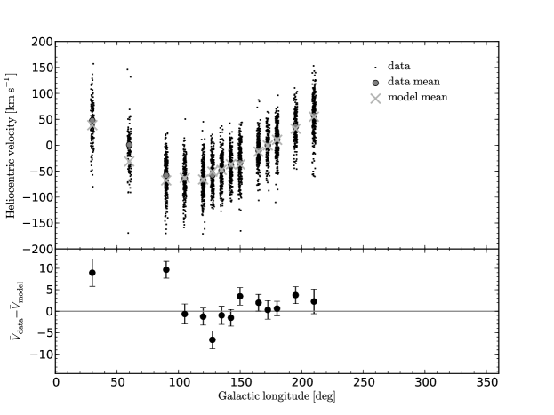
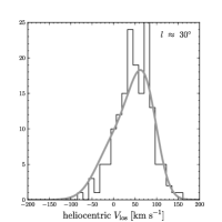
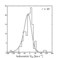
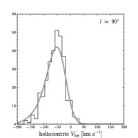
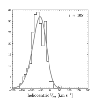
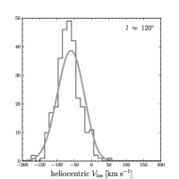
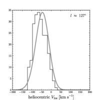
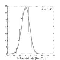
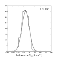
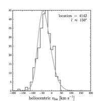
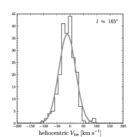
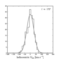
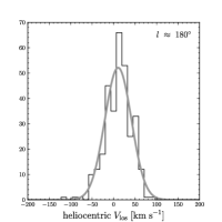
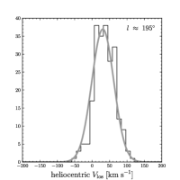
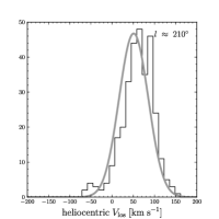
We compare the best-fit flat-rotation curve model with the data in Figures 7 and 8. Figure 7 shows the raw heliocentric velocities versus Galactic longitude for all of the stars in the sample, as well as the mean for each field, and the prediction for the mean from the best-fit model. This “model mean” is computed by constructing the predicted line-of-sight velocity distribution using Equation (2) and then calculating its mean. The full predicted line-of-sight velocity distribution for each field is shown in Figure 8 as the smooth curve, which is to be compared with the histogrammed data points for each field. It is clear from Figure 8 that the fits capture the overall smooth features of the distribution of line-of-sight velocities in each field, including any asymmetry in the distribution. However, it is also obvious that some of the model predictions are shifted from the observed histograms. This effect also appears in the comparison between the data mean and model mean for each field in the lower panel of Figure 7. There appears to be a distinct pattern in these residuals. Thus, the best-fit axisymmetric model fails to account for smooth deviations in the velocity field. These deviations are likely due to non-axisymmetric streaming motions, which are expected at this level of accuracy; We discuss this further in 5.3. With the exception of the field, the data seem to follow the smooth velocity distribution quite well, albeit somewhat shifted on average.
4.2. Systematics
The basic models presented in the previous section are potentially subject to systematic uncertainties, which we discuss in this section. These uncertainties are mainly related to the distances of the stars in our sample, as these are obtained from somewhat uncertain models of the color–magnitude distribution of giant stars in the near-infrared and bands. We discuss here the influence of our assumed value for the scale length of the stars, of potential systematic offsets in the preliminary APOGEE metallicities used to inform the photometric distances, of systematic distance uncertainties, and of the impact of mis-estimated interstellar extinction and absorption. We also discuss the effect of binary contamination, of using a different set of stellar isochrones for distance estimation, and of modeling the data using many underlying populations of stars, with velocity dispersions smoothly varying with age.
In our fits, we have simply assumed a value of for the radial scale length, , of the sample of stars used in the analysis. This assumption is based on the fact that, locally, the dominant solar-metallicity disk population has this scale length (Bovy et al., 2012c). The parameter enters our analysis in two ways, the first being in the asymmetric-drift correction (Equation (5)), and the second being in the prior on the distance distribution (Equation (A1)). The former of these is the most important for determining . Changing to —which is highly unlikely, given that such a short scale length is not observed for any of the metal-rich, “thin disk” populations in the solar neighborhood (Bovy et al., 2012c)—increases the best-fit value to for a model with a flat rotation curve, and to for a power-law rotation curve. Increasing to decreases the best-fit value to . Similar changes happen for the mock data sets described in Appendix B. Therefore, we conclude that the assumed radial scale length has a negligible influence on the inferred .
To determine the influence of systematic offsets in the metallicities used in the photometric distances, we have performed fits allowing for a single metallicity offset, , for all of the stars in the sample, for a model with a flat rotation curve. We find that the best-fit , but the best-fit value of is unchanged, as is its uncertainty (see Figure 5 for the – PDF). Although an offset of might seem large, this offset should not be thought of as a measurement of for the stars in our sample, because the photometric-distance PDFs, such as that in Figure 11, are relatively insensitive to large changes in , especially at the high-metallicity end. We have also performed a fit with a different for inner () and outer-disk fields. Such a fit finds for the outer-disk fields, and for the inner-disk fields, with a best-fit ; see Figure 5 for the full PDF of the and . As discussed previously, the photometric-distance PDFs are largely insensitive to changes in at high ; the Padova isochrones also have an upper limit of , such that increasing a star’s beyond this has no effect, because we then use . Therefore, even a change of has a negligible influence on the inner, high-metallicity, disk fields. In none of these fits is our inferred range for affected.
Similarly, we have performed fits allowing for a single distance-modulus offset, , to be applied to all of the stars in our sample, or for a separate offset for inner- and outer-disk fields. In the former case, we find , corresponding to a % distance offset, without any influence on the inferred value of . In the inner/outer offset fit, we find 23% smaller distances at , and 20% larger distances in the outer disk, again with a negligible influence on the best-fit (), but with a second minimum around , and a wider PDF that is, however, at at 99% confidence. A more physical effect is to allow for an offset in the extinction, , again using a single offset for the whole sample, or splitting the sample into inner- and outer-disk fields. A single extinction offset is well-constrained to be small: . Similarly, the best-fit extinction offset in the outer disk is , while in the inner disk we find some evidence for mis-estimated extinction, with . In both of these cases, the best-fit increases by or less, and the uncertainties remain approximately the same (see Figure 5).
As discussed in 2, we do not limit the sample to stars for which multiple velocity epochs are available that indicate that they are not part of a multiple system. Such a cut significantly reduces the longitudinal coverage of our sample. When we do apply this cut, we find that the best fits for and all other parameters are unchanged from the results for our basic flat-rotation-curve model in 4.1, albeit with larger uncertainties. We find in particular that , but the uncertainties in the position and velocity of the Sun are much increased.
In Appendix A, we describe how we employ Padova isochrones to estimate photometric distances to the stars in our sample. When instead we use isochrones from the BaSTI library (Pietrinferni et al., 2004), using the filter transformation from Carpenter (2001) to transform to the -band filter used by BaSTI, we find that the results of our basic models (both with a flat and a power-law rotation curve) are essentially unchanged (with changes in of about ).
To determine whether our results change when we fit the data as a mix of multiple stellar populations, with velocity dispersions varying from that of a young population to that of the oldest disk population, we have performed a fit where the likelihood for in Equation (1) is generalized to
| (10) |
where is the single-Gaussian population model used before, with dispersion at age
| (11) |
and using an exponentially-declining star-formation history, such that . This model follows the fit of Aumer & Binney (2009) in the solar neighborhood. We use a mix of 20 equally age-spaced populations between and , and find , showing that this alternative model does not change our results; the full – PDF is shown in Figure 5. This model has , as expected for the old, “thin disk” population.
5. Discussion
5.1. Effect of Non-Axisymmetric Features
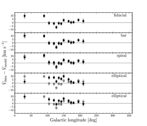
In the fits in 4, we have assumed axisymmetric models for the velocity field in the Galactic disk. However, the Milky Way is known to have some non-axisymmetric structures, such as the central bar (Blitz & Spergel, 1991; Binney et al., 1991), spiral arms (e.g., Drimmel & Spergel, 2001), and a potentially triaxial halo (Law et al., 2009), that may influence the measurement performed in this paper. Because we use a warm disk population as dynamical tracers, we can expect the influence of any non-axisymmetry to be smaller than for the colder gas tracers used in other studies (e.g., Levine et al., 2008), because warm tracers respond less strongly to non-axisymmetric perturbations to the Milky Way potential than cold tracers (Lin et al., 1969).
We have calculated the velocity field for a warm tracer population in various non-axisymmetric models (see J. Bovy, 2013, in preparation, for full details). We follow the procedure of Dehnen (2000) and Bovy (2010) to calculate the velocity distribution at a given position for a given non-axisymmetric model for the disk, by performing backward orbit integrations until before the onset of the non-axisymmetric perturbation in an axisymmetric disk. At that time, the distribution function of the pre-existing axisymmetric disk is evaluated. By the conservation of phase-space density, this probability is equal to the current probability of the phase-space starting point of the orbit integration. We assume a flat rotation curve for the axisymmetric part of the potential, and we model the initial, axisymmetric distribution function as a Dehnen distribution function (Equation (6)) with a velocity dispersion of , a radial scale length of and a dispersion scale length of . These parameters are close to the best-fit parameters for the APOGEE tracer population.
We calculate the mean velocity field for the bar model of Dehnen (2000), and use it to construct the mean, non-axisymmetric field. This field is then applied as part of the model, and the result for the mean line-of-sight velocity in each field is shown in Figure 9—there is of course much more discretionary power in the full distribution functions. In the same manner, we calculate the mean field for a two-armed logarithmic spiral with a fractional potential-amplitude of 1% of the background, axisymmetric potential, a pitch angle of , an angular frequency of (placing the Sun near the : inner Lindblad resonance), and an angle between the Sun–Galactic-center line and the line connecting the peak of the spiral pattern at the solar radius of . We do the same for models with a flat elliptical (stationary, ) distortion to the potential (see Kuijken & Tremaine 1994), with a fractional amplitude of and position angles of and with respect the the Sun–Galactic center line. All of these perturbations were adiabatically grown. We see in Figure 9 that the influence of the bar and spiral structure is negligible in the mean velocity field. An elliptical, , perturbation could distort the mean velocity field in a way that would affect our analysis. Naively, the model in the bottom panel of Figure 9 significantly reduces the residuals between the best-fit and the data .
It is clear that the data used in this paper could be used to constrain non-axisymmetric perturbations to the axisymmetric potential assumed here. We defer a full treatment of this to a subsequent paper.
5.2. Comparison with Other Determinations of the Local Circular Velocity
There have been many previous determinations of the local circular velocity, and we discuss here how our new measurement compares to these. Determinations of the local circular velocity can be roughly divided into two groups: measurements of the Sun’s velocity with respect to an object or population assumed to be at rest with respect to the Galactic center (e.g., Sgr A∗ or a population of halo objects), or direct measurements of the local radial force (e.g., by determining the Oort constants or the orbit of a stream of stars). The former directly measure the Sun’s Galactocentric velocity, , but must assume a value for the Sun’s motion with respect to the circular orbit at to arrive at . The most direct measurement of this kind is the combination of the precisely measured proper motion of Sgr A∗ (Reid & Brunthaler, 2004) with the distance to the Galactic center determined from the Keplerian orbits of S stars in the innermost parsec (Ghez et al., 2008; Gillessen et al., 2009). These measurements give , which combined with the proper motion of Sgr A∗ of , yields a total solar velocity of . As noted before, this result is entirely consistent with our inferred value of the angular motion of the Galactic center, and with our . The discrepancy between the value of in Ghez et al. (2008) (or higher measurements also based on the proper motion of Sgr A∗) and our is therefore entirely due to our different value for the solar velocity with respect to , and intrinsically these measurements are consistent. Similarly, the recent measurements of and using the kinematics of the Sgr stream (Carlin et al., 2012) are consistent with our measurement of the solar velocity.
Measurements based on the Oort constants (e.g., Feast & Whitelock, 1997), or the dynamics of a cold stellar stream (Koposov et al., 2010), also indicate that . The measurement of the Oort constants from Hipparcos proper motions by Feast & Whitelock (1997) directly measure the angular frequency of the local circular orbit, independent (in principle) from the solar motion: . This value is consistent with our determination (see Table 4) . The determination of of Koposov et al. (2010) from fitting an orbit to the cold GD-1 stellar stream at is clearly consistent with our measurement, although note that they assumed the value for the solar motion from Dehnen & Binney (1998).
The recent measurement of , from the kinematics of masers in the Galactic disk (Reid et al., 2009), was shown to have an overly optimistic precision by Bovy et al. (2009a), who concluded from a more general model for the distribution function of the masers that these data only imply . The measurement of from the maser kinematics also assumes that is given by plus the locally-determined solar motion of . Apart from indicating a high value for , albeit with a large uncertainty, the masers were also found to be lagging with respect to circular motion by about , a large offset for a young and relatively cold tracer population. This offset cannot be explained by the asymmetric drift and it is physically implausible since it requires the masers to have more eccentric orbits than most of the young stars (McMillan & Binney, 2010). Requiring the masers to be on circular orbits assuming a flat rotation curve leads to a solar motion of and (McMillan & Binney, 2010), in good agreement with our measurements. Our measurement, however, relies on the theoretically well-motivated asymmetric-drift correction that is a direct consequence of the collisionless Boltzmann equation.
Therefore, we conclude that our measurement of is consistent with previously reported values. Compared to other determinations, our measurement of is one of the most highly precise, and unlike many other measurements, it does not require assumptions about the relation between the solar motion and .
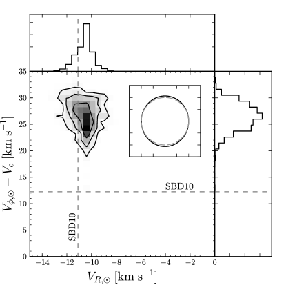
Our data strongly rule out that the Milky Way’s circular velocity at the solar radius is . Marginalizing over all of the systematics discussed in 4.2, at confidence. Fixing to with or leads to a best-fit with much larger : () and (), respectively.
5.3. Implications for the Motion of the LSR
We found in 4, in both the flat- and power-law-rotation-curve models, that the Sun’s velocity with respect to the center of the Galaxy—a distinct parameter from in our fit—is larger than by . Defining the Rotational Standard of Rest (RSR; Shuter 1982) as the circular velocity in the axisymmetric approximation to the full potential, this solar motion with respect to the RSR is much larger than that measured by applying Strömberg’s asymmetric-drift relation to local samples of stars. The asymmetric-drift relation is used to estimate the velocity of the zero-dispersion orbit by extrapolating the relation given in Equation (5) from warmer samples of stars to ; it is this zero-dispersion orbit that is typically what is meant by the LSR (Fich & Tremaine, 1991). Such analyses of the Hipparcos data yield a solar motion with respect to the LSR that is somewhere between and (Dehnen & Binney, 1998; Hogg et al., 2005; Schönrich et al., 2010); is also the offset of the average rotational velocity of nearby stars (e.g., Allende Prieto et al., 2004). The discrepancy between our determination of the solar velocity with respect to the RSR, and that with respect to the LSR, is clearly shown in Figure 10, where the PDF for is shown for the flat-rotation curve model, together with the locally-measured motion with respect to the LSR of Schönrich et al. (2010). The analogous figure for the power-law rotation-curve fit has an essentially identical appearance. It is clear that the locally-measured solar motion is not equal to our globally-measured solar motion to very high significance. Or, equivalently, the motion of the RSR is not the same as that of the LSR: the LSR seems to rotate faster than the RSR.
This discrepancy may result from a breakdown in the assumptions of the locally-measured solar motion using Strömberg’s asymmetric-drift relation. As convincingly shown by Schönrich et al. (2010), the neglect of the radial metallicity gradient in the analysis of Dehnen & Binney (1998) leads to a correction of , but further improvements in the chemical-evolution model of Schönrich et al. (2010) might lead to further corrections. The local velocity distribution has also long been known to contain various streams or “moving groups” (e.g., Kapteyn, 1905; Schwarzschild, 1907; Eggen, 1986; Dehnen, 1998; Bovy et al., 2009b) that are likely of a dynamical origin (Bensby et al., 2007; Famaey et al., 2008; Bovy & Hogg, 2010; Sellwood, 2010) and contain a significant fraction of the nearby stars (Bovy et al., 2009b). These moving groups make an accurate determination of the solar motion challenging. As such, the locally-determined correction for the Sun’s motion with respect to the LSR may well be incorrect by or more. A solar motion of rather than is not much more unlikely given the distribution function for a population: using a Dehnen distribution function (Equation (6)) with a radial dispersion of (Equation (11)) and assuming our best-fit model gives and .
However, if Strömberg’s relation leads to a solar motion with respect to the LSR that is different from the globally-determined solar motion with respect to the RSR, the most straight-forward interpretation is that LSR’s orbit is not circular, but deviates from circularity by about because of large-scale, non-axisymmetric streaming motions. The deviation cannot be much larger than this value, as the radial component of the solar motion as determined from local samples agrees with our global measurement. As our measurement of the circular velocity is mainly at azimuths , this deviation must happen over this angular scale.
There is mounting evidence for the existence of streaming motions in the Galactic disk of this magnitude. There has been a long-standing discrepancy of between the rotation curves determined from first () and fourth () quadrant tangent-point measurements (e.g., Kerr, 1962; Gunn et al., 1979; Levine et al., 2008), which could indicate streaming motions. Similarly, the analysis of the extreme line-of-sight velocity of HI emission toward leads to differences in of approximately , albeit with large uncertainties (Knapp et al., 1979; Jackson & Kerr, 1981; Jackson, 1985). The fact that the maximum line-of-sight velocity in both CO and 21-cm data reaches zero at , rather than at , has been used to argue that the LSR moves ahead of with a speed of (Shuter, 1982; Clemens, 1985), similar to the offset we find. More recently, an analysis of line-of-sight velocities from the RAVE has found a gradient, , in the mean radial velocity, , of , and large streaming motions in both and the mean tangential velocity, , within a few from the Sun (Siebert et al., 2011).
As a simple exploration of this possibility, we have computed the closed orbit at in a model for the Milky Way disk where this streaming motion is due to ellipticity of the disk, following Kuijken & Tremaine (1994). We use a flat rotation curve, with a perturbation of constant ellipticity having an amplitude of . Such a perturbation could arise if, for example, the halo is triaxial (e.g., Law et al., 2009). The closed orbit is shown to scale in the inset in Figure 10; it has an eccentricity of 0.06.
Regardless of the origin of the discrepancy between our globally-measured solar motion and the locally-measured value, our larger preferred value of means that the Sun is likely closer to the pericenter of its orbit around the Galactic center than previously believed. Revising upward by increases the eccentricity of the Sun’s orbit to from and increases its mean Galactocentric radius to from . Such a large mean radius increases the tension between the Sun’s high metallicity compared to local stars (Wielen et al., 1996), although the peak of the local metallicity distribution may be closer to solar metallicity than previously believed (e.g., Casagrande et al., 2011).
Finally, we address what our results imply for dark-matter direct-detection experiments, and for correcting the motion of Galactic and extra-galactic objects for the motion of the Sun. Both of these applications essentially require knowledge of the total Galactocentric solar velocity, , to transform velocities into the Galactocentric (dark-matter-halo) rest frame222The one exception is that in the Standard Halo Model, the velocity dispersion of the isothermal halo is given by . However, the velocity dispersion of the halo is better determined directly from observations than by using this assumption.. Although this motion is often decomposed as plus the Sun’s motion with respect to , our results in this paper show that this is unnecessarily dangerous, as it requires the strong assumption that the LSR is on a circular orbit, such that , where the final term is the solar velocity with respect to the LSR. Our results in 4 strongly rule out that this assumption holds for the currently accepted solar motion of . However, this approach is entirely unnecessary for correcting velocities to the Galactocentric rest frame, as the proper motion of Sgr A∗ combined with the “clean” estimate of from Galactic-center dynamics shows that , which agrees with our measured value of . Adopting a standard for correcting velocities for the Sun’s motion, and decoupling this correction from the question of the true value of , would therefore be helpful.
5.4. Implications for the Mass of the Milky Way
We can use our measurement of the inner rotation curve of the Milky Way to estimate the Milky Way’s total dark-halo mass. We combine the measurements in this paper with those of the Milky Way’s outer rotation curve () of Xue et al. (2008) (specifically, taking the measurements using simulation II in Table 3 of that paper). Based on Figure 6 and Table 4, we add our measurement as a flat rotation curve with , evaluated at three radii with uncertainties of , , and at , , and , respectively (removing the measurements at and from Xue et al. 2008). We also use our recent measurements of the local density of dark matter, (Bovy & Tremaine, 2012), and of the disk scale length, (Bovy et al., 2012b), revising the measurement from the latter paper downward to correct for the influence of the dark halo on that measurement.
We model the Milky Way’s potential as the combination of a bulge component with a Hernquist profile with a scale length of , a disk component with a scale height of (Bovy et al., 2012a) and a scale length that is a free parameter, and a Navarro-Frenk-White halo (NFW; Navarro et al. 1997), with a scale radius that is a free parameter (i.e., without constraint on the concentration). The relative contributions of these three components are free parameters. We then fit the data given in the previous paragraph, and we find that . The total mass of the Milky Way is .
This “low” estimate for the mass of the Milky Way likely makes it less massive than M31, which has an estimated dark-halo mass of (Watkins et al., 2010). This measurement leads to a combined mass for the Local Group of , which is consistent with the Local-Group-timing-argument within the large cosmic scatter (van der Marel et al., 2012). Our measurement of combined with its estimated -band magnitude of mag makes the Milky Way underluminous with respect to the Tully-Fisher relation of external spiral galaxies by about (see Flynn et al., 2006).
6. Conclusion
In this paper, we have measured the Milky Way’s rotation curve over the range from the new APOGEE data set of kinematically-warm stellar tracers at large distances from the Sun. Our measurement is not “clean”, in the sense of being a geometric measurement such as that provided by tangent-point observations of HI emission or by a measurement of the Sun’s motion relative to an object assumed to be at rest with respect to the Galactic center. Because we use a warm stellar population, we must correct for the offset between the average rotational velocity of this population and the circular velocity—the asymmetric drift—using a dynamical Jeans model. However, the fact that our measurement uses a dynamical effect, rather than being purely geometric, has the advantage that we unambiguously measure in the sense of the radial force at , and that we can measure the solid-body-rotation contribution to the rotation curve, in contrast to HI measurements.
Our main results are discussed in 4. We find that the Milky Way’s rotation curve is approximately flat over , with . Table 4 summarizes our results, and provides some alternative representations, such as the Oort constants, the local rotational frequency, and the contribution of the non-flatness of the rotation curve to a cylindrical-Poisson-equation determination of the local surface-mass and dark-matter densities. We simultaneously measure the Sun’s velocity in the Galactocentric rest frame—these are independent free parameters in our model—and find that and the angular motion of the Galactic center . These values are consistent with previous studies. Our measurement of then leads to a solar offset from that is larger than the locally-measured value (; Schönrich et al., 2010) by . This result may indicate that the challenging local measurement of the solar motion is incorrect or that the solar velocity is influenced by non-axisymmetric streaming motions that put the LSR on a non-circular orbit.
Looking forward, we expect to accurately measure the atmospheric parameters and abundances other than from the high-resolution APOGEE spectra in the near future. This will improve the measurements described in this paper by (a) providing better dwarf/giant separation, (b) allowing for more direct and more precise distances to be derived, and (c) letting the analysis be conducted on different chemically-defined populations of stars. In particular, this will allow for a more detailed investigation into the signatures of non-axisymmetric dynamics in our data.
The data upon which the measurements presented in this paper are based will be released as part of SDSS-III’s Data Release 10 in the summer of 2013.
Appendix A Photometric Distance PDFs for Giant Stars
In this appendix, we describe the calculation of the photometric-distance distributions for the stars in our sample. The photometric-distance PDF for each star is the combination of the probability of its observed photometry, given a model for the color–absolute-magnitude distribution of giant stars, and a prior on the distance. Thus, we write
| (A1) |
where is the distance modulus, and is the Jacobian for the coordinate transformation , because we have anticipated that the distance prior is written in Galactocentric cylindrical coordinates . This prior is an exponential distribution in , ; our sample is sufficiently close to the plane that vertical density gradients are unimportant (see Figure 2). We have implicitly assumed that the prior does not depend on . Our fiducial model has kpc, as is appropriate for the metal-rich disk stars that make up our sample (Bovy et al., 2012c).
In Equation (A1), we have also anticipated that we obtain the probability of the observed photometry of the star, given its distance from a model for the isochrones of giants, combined with a model for the distribution along the isochrone from an initial-mass-function model; this probability is labeled as ‘iso’. We only use the color and the magnitude , as little is gained by adding or separately, and we compute the density in the color–absolute-magnitude plane for a given age and metallicity (which constitutes a single isochrone) by counting the number of stars generated from an initial mass function in small boxes in – . For stars in our sample, we find the nearest (assuming ) on a grid with a spacing, and we average Padova isochrones for metallicities , and , except at the edges of the grid at and . We average over age by assuming a constant star-formation rate up to 12 Gyr (except for the fit in 4.2 with multiple populations, where we use an exponentially-declining star-formation rate). We use a lognormal Chabrier (2001) model for the IMF (but the resulting distance PDFS are essentially the same when using a Kroupa 2003 IMF). The resulting density for a star with solar metallicity is shown in Figure 11. For a given distance and , the probability of a star’s magnitude given its color is evaluated by computing its absolute magnitude and evaluating a density like the one shown in Figure 11.
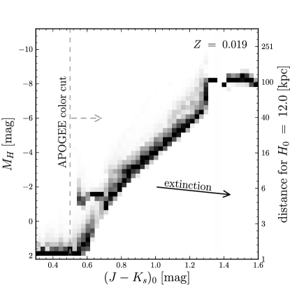
The distribution is relatively insensitive to changes in at high metallicity (), where of our sample lies. Thus, for the majority of the stars in our sample, the photometric distance PDF does not strongly depend on the measured and resembles Figure 11.
Also shown in Figure 11 is the direction that extinction moves objects in color and magnitude. In contrast to the case for the main sequence, this direction is at a large angle with the locus of the giant branch, such that under- or over-estimated extinction values can significantly change the photometric-distance PDF. The length of the extinction arrow in this figure is the median extinction in for the sample (0.45 mag).
Appendix B Analysis Tests on Mock Data Samples
| Parameter | Data / Mock input | Mock 1 | Mock 2 | Mock 3 | Mock 4 | Mock 5 | ||||||
|---|---|---|---|---|---|---|---|---|---|---|---|---|
| 5 | ||||||||||||
| 0.06 | ||||||||||||
| … | ||||||||||||
Note. — The final line of this table has the difference in per degree-of-freedom between the best-fit to the mock data set and the best-fit to the real data. Parameters are as in Table 4.
| Rotation curve | Parameter | Data / Mock input | Mock 1 | Mock 2 | Mock 3 | ||||
|---|---|---|---|---|---|---|---|---|---|
| power-law | |||||||||
| … | |||||||||
| 1.0 | |||||||||
| linear | 12 | ||||||||
| … | |||||||||
| cubic | |||||||||
| … | 1 | 1 | |||||||
| … | |||||||||
| … | 0.02 | ||||||||
| 0.05 | |||||||||
Note. — Parameters in this table are as in Table 4.
In this section, we perform extensive mock data analyses to test the methodology and approximations described in 3, and to determine at what level the data are sensitive to changes in the Galactic parameters. We create mock data sets by re-sampling the line-of-sight velocity for each data point from its PDF (Equation (1)) in the best-fit model with a flat rotation curve for the real data (Table 4). However, rather than using the simple Gaussian-with-asymmetric-drift-offset model, we sample from a Dehnen distribution function (Equation (6)), with a radial scale length of , and a radial-velocity-dispersion scale length taken from the best-fit model. Because the Dehnen distribution function has built-in, we do not use the best-fit . For a Dehnen DF, the marginalization of the planar velocity distribution over the component of the velocity that is tangential to the line-of-sight cannot be done analytically, and we numerically integrate over this component. We do not add any observational error to the mock line-of-sight velocities, as the observational uncertainties are vanishingly small (see 2). In this manner we produce five mock data sets that are exactly like the real data, except for the line-of-sight velocities.
We apply the exact same fitting procedure to the mock data as is used for the real data. We fit the five mock data sets with a flat-rotation curve model, and obtain the best-fits and uncertainties given in Table 6 (for comparison, this table also includes the best-fit model for the real data that was used to generate the mock data). We see that the true values for the parameters of interest are recovered well by the methodology of 3. We also see that the uncertainty ranges on the Galactic parameters are similar, both in size and asymmetry, to those derived for the real data. Therefore, the best-fit parameters do not appear to be biased by the approximate methodology used in this paper, and the uncertainties are as should be expected from these mock data tests.
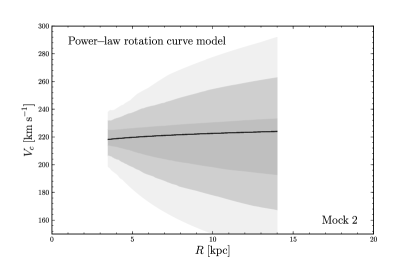
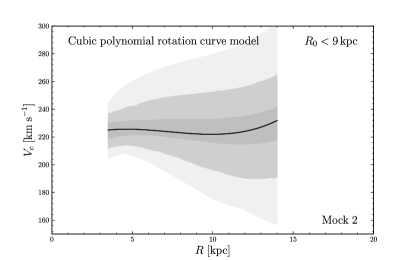
We also fit models with a non-flat rotation curve to the mock data sets. We only do this for three of the mock data sets; the results for fitting a power-law rotation curve, or a linear or cubic polynomial curve, are given in Table 8. We see that, in these cases, the Galactic parameters are recovered within the uncertainties, with perhaps a slight bias of a few in the best-fit parameters, although the (asymmetric) PDFs for the best-fit parameters do contain the “true” values within the 68% confidence intervals given. Again, the size of the uncertainties on the best-fit parameters for the mock data are similar to those found for the real data in Table 4.
In Figure 12, we show for one of the mock data sets the same representation of the constraints on the shape of the rotation curve as is given for the real data in Figure 6. Comparing these two figures, we see that the constraints are similar, with the real data giving a slightly narrower range around the best-fit, which is approximately flat. It is clear that around , the constraints on the rotation curve from the current APOGEE data become weak, so we limit our discussion to in this paper.
References
- Allende Prieto et al. (2004) Allende Prieto, C., Barklem, P. S., Lambert, D. L., & Cunha, K. 2004, A&A, 420, 183
- Aumer & Binney (2009) Aumer, M. & Binney, J. J. 2009, MNRAS, 397, 1286
- Bensby et al. (2007) Bensby, T., Oey, M. S., Feltzing, S., & Gustafsson, B. 2007, ApJ, 655, 89
- Bertelli et al. (1994) Bertelli, G., Bressan, A., Chiosi, C., Fagotto, F., & Nasi, E. 1994, A&AS, 106, 275
- Binney et al. (1991) Binney, J., Gerhard, O. E., Stark, A. A., Bally, J., & Uchida, K. I. 1991, MNRAS, 252, 210
- Binney & Tremaine (2008) Binney, J. & Tremaine, S. 2008, Galactic Dynamics: Second Edition (Princeton University Press)
- Blitz & Spergel (1991) Blitz, L. & Spergel, D. N. 1991, ApJ, 379, 631
- Bonatto et al. (2004) Bonatto, C., Bica, E., & Girardi, L. 2004, A&A, 415, 571
- Bovy et al. (2009a) Bovy, J., Hogg, D. W., & Rix, H.-W. 2009a, ApJ, 704, 1704
- Bovy et al. (2009b) Bovy, J., Hogg, D. W., & Roweis, S. T. 2009b, ApJ, 700, 1794
- Bovy (2010) Bovy, J. 2010, ApJ, 725, 1676
- Bovy & Hogg (2010) Bovy, J. & Hogg, D. W. 2010, ApJ, 717, 617
- Bovy et al. (2012a) Bovy, J., Rix, H.-W., & Hogg, D. W. 2012a, ApJ, 751, 131
- Bovy et al. (2012b) Bovy, J., Rix, H.-W., Hogg, D. W., Beers, T. C., Lee, Y. S., & Zhang, L. 2012b, ApJ, 755, 115
- Bovy et al. (2012c) Bovy, J., Rix, H.-W., Liu, C., Hogg, D. W., Beers, T. C., & Lee, Y. S. 2012c, ApJ, 753, 148
- Bovy & Tremaine (2012) Bovy, J. & Tremaine, S. 2012, ApJ, 756, 89
- Carignan et al. (2006) Carignan, C., Chemin, L., Huchtmeier, W. K., & Lockman, F. 2006, ApJ, 641, L109
- Carlin et al. (2012) Carlin, J. L., Majewski, S. R., Casetti-Dinescu, D. I., et al. 2012, ApJ, 744, 25
- Carpenter (2001) Carpenter, J. M. 2001, AJ, 121, 2851
- Casagrande et al. (2011) Casagrande, L., Schönrich, R., Asplund, M., et al. 2011, A&A, 530, 138
- Chabrier (2001) Chabrier, G. 2001, ApJ, 554, 1274
- Churchwell et al. (2009) Churchwell, E., Babler, B. L., Meade, M. R., et al. 2009, PASP, 121, 213
- Clemens (1985) Clemens, D. P. 1985, ApJ, 295, 422
- Dehnen (1998) Dehnen, W. 1998, AJ, 115, 2384
- Dehnen & Binney (1998) Dehnen, W. & Binney, J. J. 1998, MNRAS, 298, 387
- Dehnen (1999) Dehnen, W. 1999, AJ, 118, 1201
- Dehnen (2000) Dehnen, W. 2000, AJ, 119, 800
- Drimmel & Spergel (2001) Drimmel, R. & Spergel, D. N. 2001, ApJ, 556, 181
- Eggen (1986) Eggen, O. J. 1986, AJ, 92, 910
- Eisenstein et al. (2011) Eisenstein, D., et al. 2011, AJ, 142, 72
- Famaey et al. (2008) Famaey, B., Siebert, A., & Jorissen, A. 2008, A&A, 483, 453
- Feast & Whitelock (1997) Feast, M. & Whitelock, P. 1998, MNRAS, 291, 683
- Fich & Tremaine (1991) Fich, M. & Tremaine, S. 1991, ARA&A, 29, 409
- Flynn et al. (2006) Flynn, C., Holmberg, J., Portinari, L., Fuchs, B., & Jahreiß, H. 2006, MNRAS, 372, 1149
- Foreman-Mackey et al. (2012) Foreman-Mackey, D., Hogg, D. W., Lang, D., & Goodman, J. 2012, arXiv:1202.3665v2 [astro-ph.IM]
- Freeman (1987) Freeman, K. C. 1987, ARA&A, 25, 603
- Frinchaboy (2008) Frinchaboy, P. M. 2008, Ph.D. thesis, Univ. Virginia
- Ghez et al. (2008) Ghez, A. M., Salim, S., Weinberg, N. N., et al. 2008, ApJ, 689, 1044
- Gillessen et al. (2009) Gillessen, S., Eisenhauer, F., Trippe, S., Alexander, T., Genzel, R., Martins, F., Ott, T. 2009, ApJ, 692, 1075
- Girardi et al. (2005) Girardi, L., Groenewegen, M. A. T., Hatziminaoglou, E., da Costa, L. 2005, A&A, 436, 895
- Girardi et al. (2010) Girardi, L., Williams, B. F., Gilbert, K. M.,et al. 2010, ApJ, 724, 1030
- Gunn et al. (1979) Gunn, J. E., Knapp, G. R., & Tremaine, S. D. 1979, AJ, 84, 1181
- Gunn et al. (2006) Gunn, J. E., et al. 2006, AJ, 131, 2332
- Hammer et al. (2007) Hammer, F., Puech, M., Chemin, L., Flores, H., & Lehnert, M. D. 2007, ApJ, 662, 322
- Hogg et al. (2005) Hogg, D. W., Blanton, M. R., Roweis, S. T., & Johnston, K. V. 2005, ApJ, 629, 268
- Jackson & Kerr (1981) Jackson, P. D. & Kerr, F. J. 1981, BAAS, 13, 538
- Jackson (1985) Jackson, P. D. 1985, in The Milky Way Galaxy, Proceedings of IAU Symposium No. 106, eds. H. van Woerden, R. J. Allen, and W. B. Burton (Dordrecht: D. Reidel Publishing Co.), 179
- Kapteyn (1905) Kapteyn, J. C. 1905, Br. Assoc. Adv. Sci. Rep. A, 257
- Kerr (1962) Kerr, F. J. 1962, MNRAS, 123, 327
- Kerr & Lynden-Bell (1986) Kerr, F. J. & Lynden-Bell, D. 1986, MNRAS, 221, 1023
- Klypin, Zhao, & Somerville (2002) Klypin, A., Zhao, H., & Somerville, R. S. 2002, ApJ, 573, 597
- Knapp et al. (1979) Knapp, G. R., Tremaine, S. D., & Gunn, J. E. 1979, AJ, 83, 1585
- Koposov et al. (2010) Koposov, S. E., Rix, H.-W., & Hogg, D. W. 2010, ApJ, 712, 260
- Kroupa (2003) Kroupa, P. 2003, MNRAS, 322, 231
- Kuijken & Tremaine (1991) Kuijken K. & Tremaine, S. 1991, in Dynamics of Disk Galaxies, ed. B. Sundelius (Göteborg: Göteborg Univ. Press), 257
- Kuijken & Tremaine (1994) Kuijken K. & Tremaine, S. 1994, ApJ, 421, 178
- Kurucz (1979) Kurucz, R. L. 1979, ApJS, 40, 1
- Law et al. (2009) Law, D. R., Majewski, S. R., & Johnston, K. V. 2009, ApJ, 703, 67
- Levine et al. (2008) Levine, E. S., Heiles, C., & Blitz, L. 2008, ApJ, 679, 1288
- Lewis & Freeman (1989) Lewis, J. R., & Freeman, K. C. 1989, AJ, 97, 139
- Lin et al. (1969) Lin, C. C., Yuan, C., & Shu, F. H. 1969, ApJ, 155, 721
- Majewski et al. (2006) Majewski, S. R., Law, D. R., Polak, A. A., Patterson, R. J. 2006, ApJ, 637L, 25
- Majewski et al. (2011) Majewski, S. R., Zasowski, G., Nidever, D. L. 2011, ApJ, 739, 25
- Marigo et al. (2008) Marigo, P., Girardi, L., Bressan, A., Groenewegen, M. A. T., Silva, L., & Granato, G. L. 2008, A&A, 482, 883
- McMillan & Binney (2010) McMillan, P. J. & Binney, J. J. 2010, MNRAS, 402, 934
- Merrifield (1992) Merrifield, M. R. 1992, AJ, 103, 1552
- Navarro et al. (1997) Navarro, J. F., Frenk, C. S., & White, S. D. M. 1997, ApJ, 490, 493
- Pietrinferni et al. (2004) Pietrinferni, A., Cassisi, S., Salaris, M., & Castelli, F. 2004, ApJ, 612, 168
- Reid & Brunthaler (2004) Reid, M. J. & Brunthaler, A. 2004, ApJ, 616, 872
- Reid et al. (2009) Reid, M. J., Menten, K. M., Zheng, X. W., et al. 2009, ApJ, 700, 137
- Schönrich et al. (2010) Schönrich, R., Binney, J. J., & Dehnen, W. 2010, MNRAS, 403, 1829
- Schönrich (2012) Schönrich, R. 2012, MNRAS, in press, arXiv:1207.3079
- Schwarzschild (1907) Schwarzschild, K. 1907, Nachr. Koniglichen Ges. Wiss. Goett., 5, 614
- Sellwood (2010) Sellwood, J. A. 2010, MNRAS, 409, 145
- Shuter (1982) Shuter, W. L. H. 1982, MNRAS, 199, 109
- Siebert et al. (2011) Siebert, A., Famaey, B., Minchev, I., et al. 2011, MNRAS, 412, 2026
- Sirko et al. (2004) Sirko, E., Goodman, J., Knapp, J. R., Brinkmann, J., Ivezić, Z., Knerr, E. J., Schlegel, D. J., Schneider, D. P., & York, D. G. 2004, AJ, 127, 914
- Skrutskie et al. (2006) Skrutskie, M. F., Cutri, R. M., Stiening, R., et al. 2006, AJ, 131, 1163
- Strömberg (1946) Strömberg, G. 1946, ApJ, 104, 12
- Toomre (1964) Toomre, A. 1964, ApJ, 139, 1217
- van de Hulst et al. (1954) van de Hulst, H. C., Muller, C. A., & Oort, J. H. 1954, BAN, 12, 117
- van der Marel et al. (2012) van der Marel, R. P., Fardal, M., Besla, G., Beaton, R. L., Sohn, S. T., Anderson, J., Brown, T., & Guhathakurta, P. 2012, ApJ, 753, 8
- Watkins et al. (2010) Watkins, L. L., Evans, N. W., An, J. H. 2010, MNRAS, 406, 264
- Wielen et al. (1996) Wielen, R., Fuchs, B., & Dettbarn, C. 1996, A&A, 314, 438
- Wilson et al. (2010) Wilson, J. C., Hearty, F., Skrutskie, M. F., et al. 2010, Proc. SPIE, 7735, 46
- Woltjer (1975) Woltjer, L. 1975, A&A, 42, 109
- Wright et al. (2010) Wright, E. L., Eisenhardt, P. R. M., Mainzer, A. K., et al. 2010, AJ, 140, 1868
- Xue et al. (2008) Xue, X. X., Rix, H.-W., Zhao, G., et al. 2008, ApJ, 684, 1143
- Zasowski et al. (2009) Zasowski, G., Majewski, S. R., Indebetouw, R., et al. 2009, ApJ, 707, 510