Kepler-47: A Transiting Circumbinary Multi-Planet System
We report the detection of Kepler-47, a system consisting of two planets orbiting around an eclipsing pair of stars. The inner and outer planets have radii 3.0 and 4.6 times that of the Earth, respectively. The binary star consists of a Sun-like star and a companion roughly one-third its size, orbiting each other every 7.45 days. With an orbital period of 49.5 days, eighteen transits of the inner planet have been observed, allowing a detailed characterization of its orbit and those of the stars. The outer planet’s orbital period is 303.2 days, and although the planet is not Earth-like, it resides within the classical “habitable zone”, where liquid water could exist on an Earth-like planet. With its two known planets, Kepler-47 establishes that close binary stars can host complete planetary systems.
The extremely precise and nearly continuous observations provided by the Kepler spacecraft (?) has enabled the detection of over 2300 planet candidates (?, ?), and over 2100 eclipsing binary stars (?, ?). A synergy of these efforts has helped establish the class of circumbinary planets, which are planets that orbit around a pair of stars (?, ?, ?). Their detection has led to a revitalized effort to understand planet formation around binary stars (?, ?). A circumbinary planet can reveal itself in two ways. If the planet’s orbital plane is favorably aligned, the planet may transit across one or both of the stars, causing a small decrease in the amount of light from the system. If the planet is sufficiently massive and close, the planet can perturb the stellar orbits (?). The most readily observable manifestation of this perturbation is a change in the times when the eclipses occur.
In contrast to a single planet orbiting a single star, a planet in a circumbinary system must transit a “moving target.” As a consequence, the time intervals between the transits as well as their duration can vary substantially. The transits can deviate from having a constant period by up to several days and can vary in duration by several hours. These transit timing and duration variations can be taken to be the signature of a circumbinary planet because no other known mechanism can cause such effects. Modeling of the timing and duration changes can be used to precisely determine the orbits of the planet and stars (?, ?, ?).
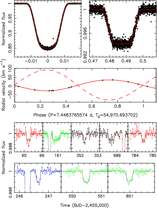
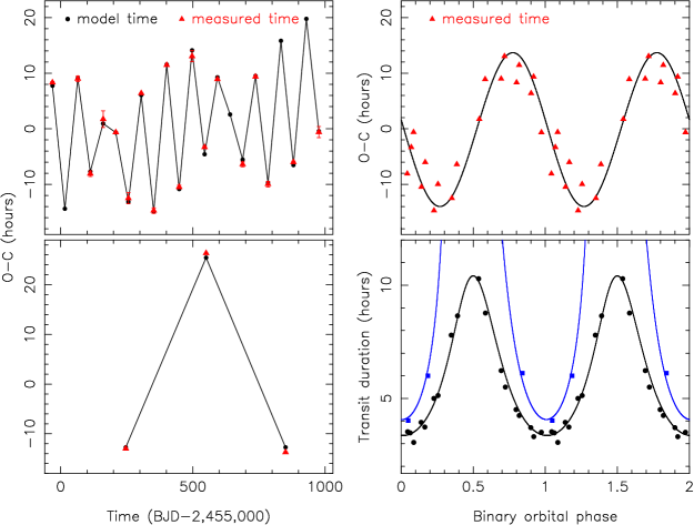
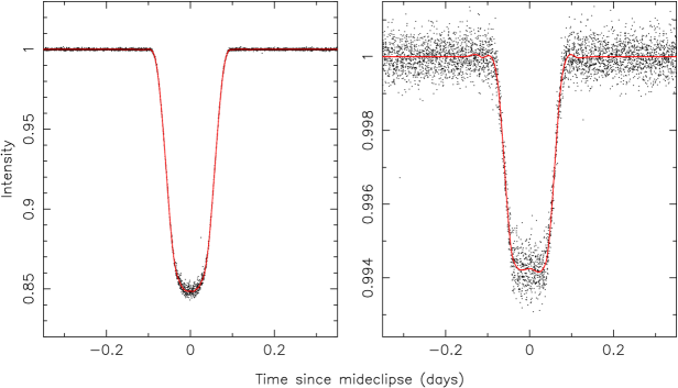
Kepler observations of the binary star system Kepler-47 (KIC 10020423, also KOI-3154) show primary eclipses (smaller and fainter star blocking the brighter, more massive “primary” star) every 7.45 days with a depth of 13%. Also present are secondary eclipses with a depth of 0.8% (Fig. 1) and a quasi-periodic modulation in the out-of-eclipse regions of % caused by star-spots on the primary star (?). The Kepler data span 1050.5 days and visual inspections of the light curve revealed the signals of two candidate circumbinary planets, with periods of and days. Three transits of the longer-period candidate (hereafter the outer planet) were readily apparent, but those of the shorter-period candidate (hereafter the inner planet) were more difficult to find because of their shallower depth. Using the predictions of a preliminary model of the system as a guide, a total of 18 transits of the inner planet were detected. The transits have timings that can deviate from strict periodicity by up to several hours and their durations vary significantly, strongly suggesting their origins are from circumbinary planets (Fig. 2). All of these events are transits over the primary star.
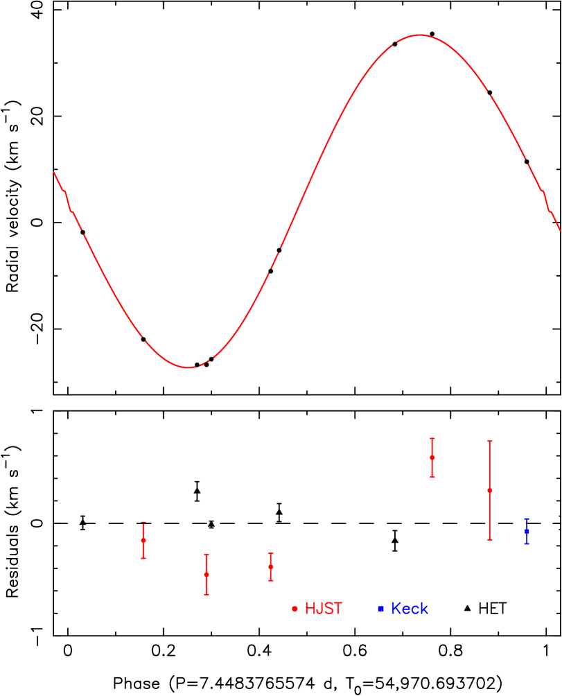
To characterize the stellar orbit, we obtained Doppler spectroscopy of the system (?, Fig. 1). Radial velocity variations of the primary star were readily detected, but the secondary star is too faint to have been measured. Usually when the radial velocity measurements of only one component in a spectroscopic binary are available, the masses of the stars cannot be uniquely determined. However, the transit times and durations provide constraints on the geometric configuration of the stellar orbits and specify the stellar mass ratio, which in combination with the primary’s radial velocities, allow both stellar masses and the physical scale to be determined.
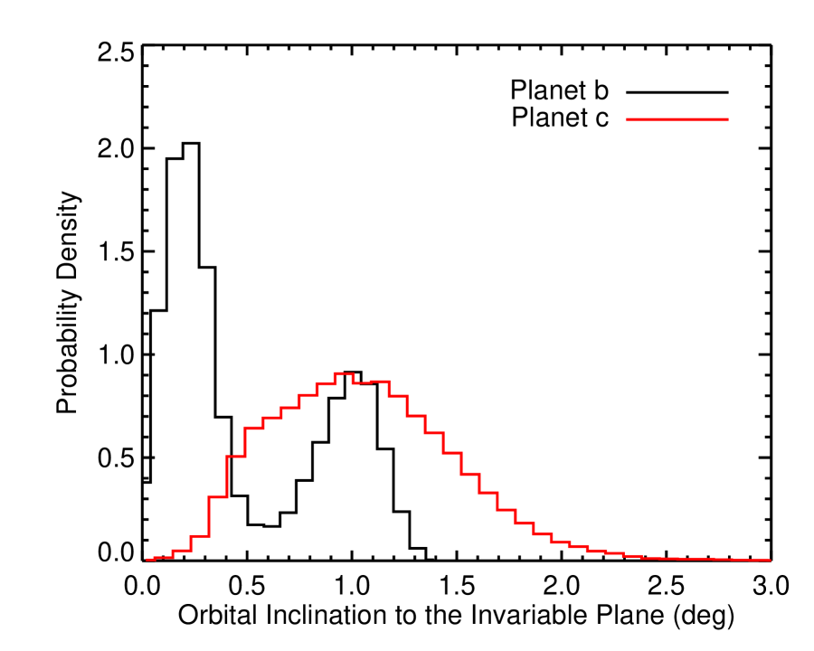
To determine the system parameters, we used a photometric-dynamical model (?) similar to that used for the four previously known transiting circumbinary planets (?, ?, ?). This model assumes spherical bodies interacting via Newtonian gravity (?), and is used to fit the radial velocity data and the Kepler time-series photometry. We determined the stellar masses as described above, and the relative sizes of the bodies from the eclipses and transits in the light curve. Information on the inclination, eccentricity, and mutual inclination of the planetary orbits is also implicit in the combination of photometric and radial-velocity data. Gravitational perturbations caused by the planets on the stars and on each other could, in principle, also constrain the masses, but for Kepler-47 the expected masses of the planets are too small to create a measurable effect over the time span of our data. The small radii of the transiting objects strongly suggests they are of planetary mass (Table 1); dynamical considerations described below make this conclusion secure.
The inner planet, Kepler-47 b, is the smallest transiting circumbinary planet yet detected, with a radius of Earth radii. Its mass is too small to be directly measured, but a upper limit of 2 Jupiter masses has been determined based on the nondetection of timing variations of the stellar orbit (?). Because the planet’s mass is unknown, its density is also unknown and it is not possible to distinguish between a rocky composition and a more volatile-enriched composition. We can make a plausible mass etimate by using both an empirical mass-radius relation based on transiting exoplanets (?) and a limited empirical mass-radius relation for planets in the Solar System (?) yielding Earth masses or Neptune masses. The planet’s 49.5-day orbital period is 6.6 times the period of the stellar binary. This is longer than the critical period (28 d) within which the planet would be susceptible to dynamical instability due to interactions with the stars (?). While this 77% margin is notably larger than for the other known transiting circumbinary planets, i.e., 14%, 21%, 24%, 42% for Kepler 16, 34, 35, and 38, respectively, the planet is still somewhat close to the instability limit, a feature shared by all known transiting circumbinary planet systems.
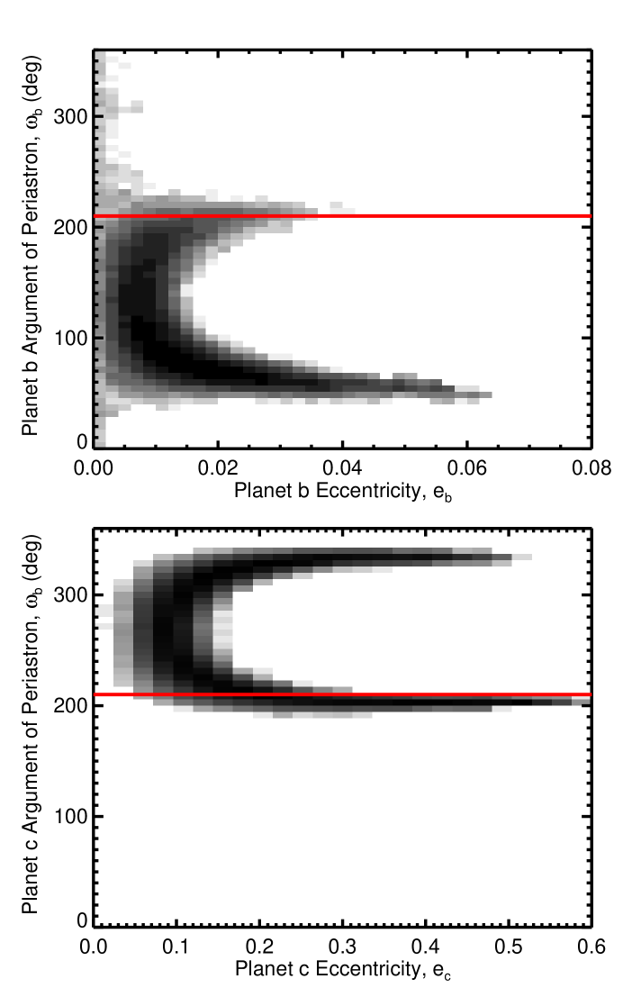
The outer planet, Kepler-47 c, has a radius of Earth radii, making it slightly larger than the planet Uranus. As before, the planet’s mass is too small to be measured directly, and we derived a upper limit of 28 Jupiter masses (?). Based on its radius, we find a plausible mass of Earth masses or Neptune masses, using these empirical mass-radius relations (?, ?). With only 3 transits currently available, the outer planet’s orbital eccentricity is poorly constrained. A perfectly circular orbit would fit the data, and a low-eccentricity orbit seems plausible given the low eccentricity of the stellar binary () and of planet b (). The photometric-dynamical model provides only an upper limit on the eccentricity, with 95% confidence, and the requirement of long-term stability only rules out eccentricities larger than 0.6 (?).
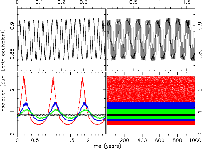
Due to the orbital motion of the stars, the outer planet is subject to variations in the incident stellar flux (i.e. insolation), even if the planet’s orbit is circular (Fig. 3). The average insolation is similar to the amount the Earth receives from the Sun: for a circular orbit it is 87.5% of the Sun-Earth insolation, and varies by %. This places Kepler-47 c well within the classical “habitable zone”, defined as the range of distances from the host star(s) where liquid water could persist on the surface of an Earth-like planet (?). While Kepler-47 c is probably a gas giant and thus not suitable for life, its location is notable as it demonstrates that circumbinary planets can exist in habitable zones. Although the definition of the habitable zone assumes a terrestrial planet atmosphere which does not apply for Kepler-47 c, large moons, if present, would be interesting worlds to investigate.
A 0.2% deep transit-like event is present at time 2,455,977.363 (BJD) that is not caused by either of the two planets. A search for additional transits has revealed several more tentative transit events (?), but we caution that the star is faint (the Kepler magnitude is 15.178), there are large modulations due to star-spots, and the data contain correlated “red” noise, making small, non-periodic transit detection challenging. The marginal evidence at the present time is insufficient to place confidence on any additional candidate planet(s).
The primary star is similar to the Sun in both mass and radius, and dominates the luminosity of the binary system, having 60 times the bolometric luminosity of the secondary star (or 176 times the brightness in the Kepler bandpass). A spectroscopic analysis gives an effective temperature of for the primary star (Table S2), with a metallicity slightly less than solar ([M/H] dex). The star’s rotation period as determined from the star-spot modulation in the light curve (?) is only 4% longer than the orbital period, suggesting that the spin and orbital angular momenta have been synchronized by tidal interactions. Supporting this interpretation, the obliquity of the primary star (the angle between the spin and orbital axes) must be smaller than about , based on the observable effects of the secondary star eclipsing star-spots on the primary star (?, ?, ?, ?, ?). Star-spot crossings also perturb the shape and depth of the primary eclipses, leading to systematic trends in the eclipse times, and limit the precision with which one can infer the planets’ masses. In addition, the loss of light due to star-spots causes eclipses to appear slightly deeper than they would for an unspotted star, biasing the determination of the stellar and planetary radii too high by a few percent.
With Kepler-47 b and c, there are six confirmed transiting circumbinary planets currently known. Their orbital periods relative to their host binary stars show no tendency to be in resonance, and their radii are Saturn-size and smaller. Given that Jupiter-size planets are easier to detect, their absence in the Kepler data suggests that the formation and migration history of circumbinary planets may disfavor Jupiter-mass planets orbiting close to the stars, in accord with (?).
The planets in Kepler-47 are expected to have formed much farther out than their present orbits, at locations where the conditions for the formation of giant planets are more favorable (?, ?). The planets have likely migrated to their current orbits as a result of interactions with the circumbinary disk. The multiplicity and coplanarity of the orbits strengthens the argument for a single-disk formation and a migration scenario for circumbinary planetary systems. However, unlike orbits around a single star, the environment around a binary star is much more dynamic and tends to augment planet-planet interactions. The relatively large distance between the orbits of the inner and outer planets in the Kepler-47 system is consistent with requirements for dynamical stability (?).
The previously detected transiting circumbinary planet systems show no evidence for more than a single planet. The multi-planet nature of the Kepler-47 system establishes that despite the chaotic environment around binary stars, planetary systems can form and persist close to the binary, and invites a broader investigation into how circumbinary planets compare to planets and planetary systems around single stars.
References and Notes
- 1. D. G. Koch, W. J. Borucki, G. Basri, N. M. Batalha, T. M. Brown, et al., Kepler mission design, realized photometric performance, and early science. Astrophys. J. 713, L79-L86 (2010).
- 2. W. J. Borucki, D. Koch, G. Basri, N. Batalha, T. Brown, et al., Kepler Planet-Detection Mission: Introduction and First Results. Science 327, 977 (2010).
- 3. N. M. Batalha, J. F. Rowe, S. T. Bryson, T. Barclay, C. J. Burke, et al., Planetary candidates observed by Kepler, III: analysis of the first 16 months of data. Astrophys. J. Suppl. Ser. submitted, arXiv:1202.5852, (2012).
- 4. A. Prša, A., N. Batalha, R. W. Slawson, L. R. Doyle, W. F. Welsh, et al., Kepler eclipsing binary stars. I. catalog and principal characterization of 1879 eclipsing binaries in the first data release. Astron. J. 141, 83 (2011).
- 5. R. W. Slawson, A. Prša, W. F. Welsh, J. A. Orosz, M. Rucker, et al., Kepler eclipsing binary stars. II. 2165 eclipsing binaries in the second data release. Astron. J. 142, 160 (2011).
- 6. L. R. Doyle, J. A. Carter, D. C. Fabrycky, R. W. Slawson, S. B. Howell, et al., Kepler-16: a transiting circumbinary planet. Science 333, 1602 (2011).
- 7. W. F. Welsh, J. A. Orosz, J. A. Carter, D. C. Fabrycky, E. B. Ford, et al., Transiting circumbinary planets Kepler-34 b and Kepler-35 b. Nature 481, 475-479 (2012).
- 8. J. A. Orosz, W. F. Welsh, J. A. Carter, E. Brugamyer, L. A., Buchhave, et al., The Neptune-sized circumbinary planet Kepler-38b. Astrophys. J. in press, arXiv:submit/0534300 (2012).
- 9. S. Meschiari, Circumbinary planet formation in the Kepler-16 system. I. N-body simulations. Astrophys. J. 752, 71 (2012).
- 10. S.-J. Paardekooper, Z. M. Leinhardt, P. Thébault, & C. Baruteau, How not to build Tatooine: the difficulty of in situ formation of circumbinary planets Kepler 16b, Kepler 34b, and Kepler 35b. Astrophys. J. 754, L16 (2012).
- 11. T. Borkovits, B. Érdi, E. Forgács-Dajka, & T. Kovács, On the detectability of long period perturbations in close hierarchical triple stellar systems. Astron. Astroph. 398, 1091-1102 (2003).
- 12. See the Supplementary Materials on Science Online.
- 13. J. A. Carter, D. C. Fabrycky, D. Ragozzine, M. J. Holman, S. N. Quinn, et al., KOI-126: A triply eclipsing hierarchical triple with two low-mass stars. Science 331, 562 (2011).
- 14. S. R. Kane, & D. M. Gelino, The habitable zone gallery. Pubs. Astron. Soc. Pac. 124, 323-328 (2012).
- 15. J. J. Lissauer, D. Ragozzine, D. C. Fabrycky, J. H. Steffen, E. B. Ford, et al., Architecture and dynamics of Kepler’s candidate multiple transiting planet systems. Astrophys. J. Suppl. Ser. 197, 8 (2011).
- 16. M. J. Holman, & P. A. Wiegert, Long-term stability of planets in binary systems. Astron. J. 117, 621-628 (1999).
- 17. J. F. Kasting, D. P. Whitmire, & R. T. Reynolds, Habitable zones around main sequence stars. Icarus 101, 108-128 (1993).
- 18. R. Sanchis-Ojeda, J. N. Winn, M. J. Holman, J. A. Carter, D. J. Osip, & C. I. Fuentes, Starspots and spin-orbit alignment in the WASP-4 exoplanetary system. Astrophys. J. 733, 127 (2011).
- 19. P. A. Nutzman, D. C. Fabrycky, & J. J. Fortney, Using star spots to measure the spin-orbit alignment of transiting planets. Astrophys. J. 740, L10 (2011).
- 20. J. M. Désert, D. Charbonneau, B.-O. Demory, S. Ballard, J. A. Carter, et al., The Hot-Jupiter Kepler-17b: discovery, obliquity from stroboscopic starspots, and atmospheric characterization. et al., Astrophys. J. Suppl. Ser. 197, 14 (2011).
- 21. R. Sanchis-Ojeda, D. C. Fabrycky, J. N. Winn, T. Barclay, B. D. Clarke, et al., Alignment of the stellar spin with the orbits of a three-planet system. Nature 487, 449 (2012).
- 22. A. Pierens, & R. P. Nelson, On the formation and migration of giant planets in circumbinary discs. Astron. Astroph. 483, 633-642 (2008).
- 23. A. N. Youdin, K. M. Krautter, & S. J. Kenyon, Circumbinary Chaos: Using Pluto’s Newest Moon to Constrain the Masses of Nix and Hydra. Astrophys. J. 755, 17 (2012).
- 24. D. R. Underwood, B. W. Jones, & P. N. Sleep, The evolution of habitable zones during stellar lifetimes and its implications on the search for extraterrestrial life. Int. J. Ast. Bio. 2, 289 (2003).
-
Kepler was selected as the 10th mission of the Discovery Program. Funding for this mission is provided by NASA, Science Mission Directorate. The Kepler data presented in this paper were obtained from the Mikulski Archive for Space Telescopes (MAST). The Space Telescope Science Institute (STScI) is operated by the Association of Universities for Research in Astronomy, Inc., under NASA contract NAS5-26555. Support for MAST for non-HTS data is provided by the NASA Office of Space Science via grant NXX09AF08G and by other grants and contracts. This work is based in part on observations obtained with the Hobby-Eberly Telescope, which is a joint project of the University of Texas at Austin, the Pennsylvania State University, Stanford University, Ludwig-Maximilians-Universität München, and Georg-August-Universität Göttingen. JAO and WFW acknowledge support from the Kepler Participating Scientist Program via NASA grant NNX12AD23G; JAO, WFW and GW also gratefully acknowledge support from the NSF via grant AST-1109928. G.T. acknowledges partial support for this work from NSF grant AST-1007992. J.A.C. and D.C.F. acknowledge NASA support through Hubble Fellowship grants HF-51267.01-A and HF-51272.01-A, respectively, awarded by STScI.
Supplementary Materials
Materials and Methods
Supplementary Text
Figs. S1 to S25
Tables S1 to S9
Full reference list
| parameter | best fit | uncertainty |
|---|---|---|
| Bulk Properties | ||
| Mass of Star A, () | ||
| Mass of Star B, () | ||
| Radius of Star A, () | ||
| Radius of Star B, () | ||
| Temperature of Star A, (K) | 5636 | 100 |
| Temperature of Star B, (K) | 3357 | 100 |
| Luminosity of Star A, () | 0.840 | 0.067 |
| Luminosity of Star B, () | 0.014 | 0.002 |
| Radius of Planet b, () | ||
| Radius of Planet c, () | ||
| Stellar Orbit | ||
| Semimajor Axis, (AU) | ||
| Orbital Period, (day) | ||
| Eccentricity, | ||
| Argument of Periapse, (Degrees) | ||
| Orbital Inclination, (deg) | ||
| Planet b Orbit | ||
| Semimajor Axis, (AU) | ||
| Orbital Period, (day) | ||
| Eccentricity (95% conf.), | ||
| Orbital Inclination, (deg) | ||
| Mutual Orbital Inclination, (deg) | ||
| Planet c Orbit | ||
| Semimajor Axis, (AU) | ||
| Orbital Period, (day) | ||
| Eccentricity (95% conf.), | ||
| Orbital Inclination, (deg) | ||
| Mutual Orbital Inclination, (deg) | ||
Supporting Online Material (SOM)
We provide additional details regarding the detection and characterization of Kepler-47 in this supplement. §1.1 gives alternate designations and other information for Kepler-47. §1.2 discusses the Kepler data preparation and detrending. §1.3 discusses how the rotational period of the primary star is derived. §1.4 discusses the ground-based spectroscopic observations. §1.5 describes how the effective temperature, gravity, and metallicity of the primary were measured. §1.6 gives an overview of how the times of mid-eclipse for the primary and secondary eclipses were measured. §1.7 discusses the effects of star-spots on the measurement of the eclipse times and other parameters. §1.8 presents measurements of the transit times and the detection of a transit event possibly due to a third planet. §1.9 gives a full discussion of the photometric-dynamical model. §1.10 presents a discussion of independent light curve modeling done with the ELC code. §1.11 discusses how upper limits on the masses of the planets were derived. §1.12 considers the long-term stability of the planetary orbits. §1.13 gives a comparison of the stellar properties with evolutionary models. §1.14 presents details of the habitable zone in Kepler-47.
1 Materials and Methods
1.1 Alternate designations, celestial coordinates, and apparent magnitudes
Kepler-47 appears in the Kepler Input Catalog (?, KIC) as KIC 10020423. Other designations include Kepler Object of Interest KOI-3154 and 2MASS J19411149+4655136. The J2000 celestial coordinates given in the KIC are , , and the apparent magnitudes are and .
1.2 Kepler data preparation and detrending
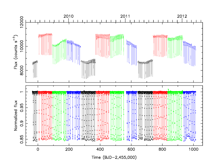
In this study we make use of data from Kepler Quarters Q1 through Q12 (May, 2009 through late March, 2012). We used the “simple aperture photometry” (SAP) provided by the Kepler pipeline and available at the Mikulski Archive for Space Telescopes (MAST). The Kepler SAP light curves show instrumental trends (?), so further processing is necessary. The detrending must be done for each Quarter separately since the object appears on a different detector module. The amount of detrending needed depends on the specific task. When modeling the eclipses and transits, a fairly aggressive detrending is used where both the instrumental trends and the spot modulations are removed. In this case, the eclipses and transits are masked out, and a high order cubic spline is fit to short segments whose end points are usually defined by gaps in the data collection due to monthly data downloads, rolls between Quarters, or spacecraft safe modes. The segments are normalized to the spline fits, and the segments are reassembled. The SAP light curves and the detrended light curve with the spot modulation removed are shown in Fig. S4. Other tasks such as spot modeling require much less aggressive detrending, in which case low-order polynomials are used to stitch together different segments across the Quarters.
The time difference between the last Q12 observation and the first Q1 observation is 1050.51 days. During that interval, Kepler was collecting data 92.55% of the time, and 44389 cadences out of the 47580 in total were flagged as good (SAP_QUALITY=0), for a duty cycle of 86.34%. Not all observations with SAP_QUALITY0 are necessarily useless, depending on the purpose, so the 86.34% duty cycle is a lower limit.
1.3 Rotational period from star-spot induced stellar variations
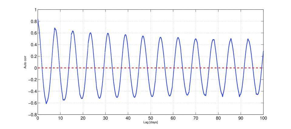
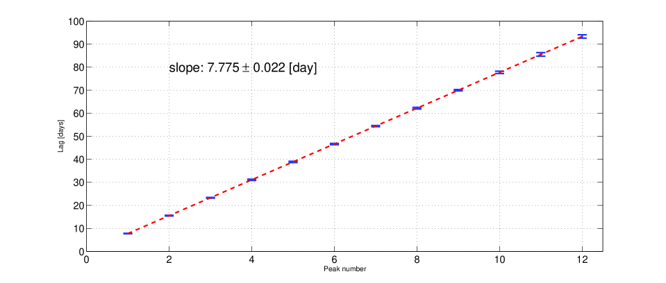
Fig. S5 shows closer-in views of the light curves from Q1, Q5, and Q9. A modulation of up to 3% in the out-of-eclipse regions due to star spots rotating into and out of view is evident. This modulation has a period that is close to, but not exactly equal to the eclipse (e.g. orbital) period. Fig. S6 depicts the autocorrelation of the cleaned detrended light curve, after the primary and secondary eclipses were removed and replaced by the value of the mean light curve with a typical random noise. The autocorrelation reveals clear modulation with a period of about 7.8 days. Presumably, the clock behind the modulation is the stellar rotation of the primary, which has brightness variation due to inhomogeneous distribution of stellar spots (as the primary star dominates the light in the Kepler bandpass, we assume it is the source of the modulation). To obtain a more precise value of the stellar rotation we measured the lags of the first 12 peaks of the autocorrelation and fitted them with a straight line as shown in Fig. S7. From the slope of the fitted line we derived a value of days as our best value for the stellar rotation period. This period is slightly longer than the orbital period of 7.448 days. It is interesting to note that the transition between synchronized and unsynchronized binaries for pre-main sequence and young stars appears between 7 and 8 days, as depicted by (?).
1.4 Spectroscopic observations
We observed Kepler-47 four times with the High-Resolution-Spectrograph (?, HRS) at the Hobby-Eberly Telescope (HET). Spectra with a resolving power of were obtained on UT 2012, April 23, May 18 & 20 and June 5. We used the “600g5822” setting of HRS that delivers a spectrum from 4814 to 6793 Å. The data were reduced with our own HRS reduction script using standard IRAF routines. We selected a total exposure of 3600 seconds per spectrum (divided into three sub-exposures of 1200 seconds each to facilitate cosmic-ray removal). The signal-to-noise (S/N) levels of the HRS spectra range from 30:1 to 55:1 at 5500 Å, depending on seeing conditions. Adjacent to every visit to Kepler-47 we also observed the Kepler field standard star HD 182488 to be used for the radial velocity determination.
In addition to the HET observations, we observed Kepler-47 six times using the Tull Coudé spectrograph (?) at the Harlan J. Smith 2.7m telescope (HJST). The data were obtained with our standard instrumental setup that covers the a wavelength range of 3760-10,200 Å and uses a 1.2 arcsecond slit that yields a resolving power of . We obtained data during the nights of UT 2012, May 1, 2, 4-6 and on June 26. Exposure times ranged from 3600 to 4800 seconds (again divided in 1200 second sub-exposures) and the S/N is typically around 14:1 at 5500Å. Each of these nights we also observed HD 182488 to serve as a radial velocity standard. The data were reduced with our own reduction scripts using standard IRAF routines. After some experimentation, it was discovered that better measurements of the radial velocities were obtained from spectra that did not have the sky background subtracted.
An additional spectrum of Kepler-47 was obtained using the 10 m Keck 1 telescope and the HIRES spectrograph (?). The spectra were collected using the standard planet search setup and reduction (?). The resolving power is at 5500 Å. Sky subtraction, using the “C2 decker” was implemented with a slit that projects to arcsec on the sky. The wavelength calibrations were made using Thorium-Argon lamp spectra.
The radial velocities of Kepler-47 were measured using the “broadening function” technique (?). The broadening functions (BFs) are rotational broadening kernels, where the centroid of the peak yields the Doppler shift and where the width of the peak is a measure of the rotational broadening. The BF analysis is often better suited for measuring radial velocities of binary stars in cases where the velocity difference between the two stars is small compared to the spectral resolution. A high quality spectrum of a slowly rotating star is needed for the BF analysis, and for this purpose we used observations of HD182488 (spectral type G8V) taken with each telescope+instrument combination. The derived radial velocities are insensitive to the precise spectral type of the template, as similar radial velocities are found when using templates of early G to late K. The adopted template radial velocity was km s-1 (?).
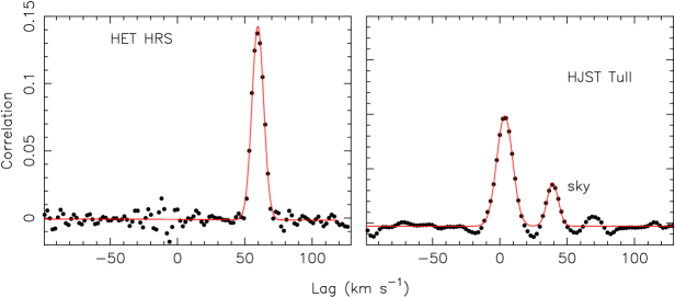
We prepared the spectra for the BF analysis by normalizing each echelle order to the local continuum using cubic splines, trimming the low signal-to-noise ends of each order, and merging the orders by interpolating to a log-linear wavelength scale. The wavelength ranges used for the final BF analysis was 4830-5770 Å for the HET spectra and 5138-5509 Å for the HJST spectra. Fig. S8 shows example BFs from HET and HJST spectra. The spectrum is single-lined, as only one peak is evident in the BFs from the HET. Some simple simulations were performed, and non-detection of a second star in the HET spectra indicates the secondary star is times fainter than the primary star, consistent with the expectations based on the eclipse depths, where a flux ratio of is expected. In the case of the HJST, two peaks are apparent. However, one of the peaks is due to the sky background since it is stationary in velocity, and changes strength relative to the other. The FWHM of the BF peaks were consistent with the instrumental broadening, which indicates the rotational velocity of the primary is at best only marginally resolved.
Gaussian functions were fit to the BF peaks to determine the relative Doppler shifts. The appropriate barycentric velocity corrections were applied and the contribution of the template radial velocity was removed, thereby placing the radial velocities on the standard IAU radial velocity scale defined by (?) and (?). The Keck HIRES pipeline automatically produces radial measurements for single stars on the IAU scale, accurate to 0.1 km s-1 or better (?). Having established Kepler-47 as a single-lined binary, we simply adopted the pipeline measurement. The radial velocity measurements for all 11 observations are given in Table S1.
1.5 Spectroscopic parameters
The effective temperature , surface gravity , the metallicity [m/H], and the rotational velocity of the primary were measured using the Stellar Parameter Classification (SPC) code (?). SPC uses a cross-correlation analysis against a large grid of model spectra in the wavelength region 5050 to 5360 Å. Since all of the absorption lines in this region are used, the SPC analysis is ideal for spectra with low signal-to-noise. The first three HET observations were combined to yield a spectrum with a signal-to-noise ratio of in the order containing the Mg b features near 5169 Å (the fourth HET observation had relatively high sky contamination and was not used). The derived spectroscopic parameters are given in Table S2.
1.6 Stellar eclipse times and corrections
The times of mid-eclipse for the primary and secondary eclipses in Kepler-47 were measured using the technique described in (?). For completeness we give most of the details here as well. Given an initial linear ephemeris and an initial estimate of the eclipse widths, the data near the eclipses were isolated and locally detrended using a cubic polynomial with the eclipses masked out. The detrended data were then folded on the linear ephemeris and an eclipse template was made by fitting a cubic Hermite spline. The Piecewise Cubic Hermite Spline (PCHS) model template was then iteratively cross-correlated with each individual eclipse event to produce a measurement of the time at mid-eclipse. After each iteration, a new PCHS model was produced by using the latest measured times to fold the data. Fig. S9 shows the folded eclipse profiles and the final PCHS models. The fits are generally good, although there is increased scatter near the middle of the primary eclipse, presumably due to the effects of star spots. Table S3 gives the eclipse times. The cycle numbers for the secondary eclipse are not exactly half integers because the orbit is eccentric.
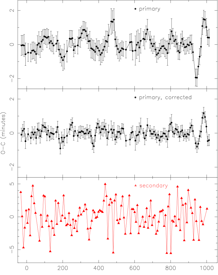
The eclipse times were fitted with a linear ephemeris and the Observed minus Computed (O-C) residual times were calculated and are shown in Fig. S10. For the primary, there are coherent deviations of up to two minutes. While not strictly periodic, there is a quasiperiod of days seen in a periodogram (Fig. S11). This modulation is most likely a beat frequency between the stellar rotation and the binary motion, similar to what is observed for Kepler-17 (?). If the secondary passes in front of a big spot during the primary eclipse, the spot anomaly will introduce a shift on the eclipse timing since the projected stellar disk of the primary on the sky will no longer have a symmetric surface brightness distribution. The shift of the eclipse time will depend on the size and position of the spot and the position on the eclipse chord. A long-lasting spot will introduce shifts in consecutive eclipses, but the shift will change with time since the spot will be at a different position on the eclipse chord at each eclipse. More specifically for this system, a spot with a period of rotation of 7.775 days will effectively recede on the transit chord each eclipse. In order to come back to the exact same position, and hence complete a full cycle in the O-C diagram, days will be needed, which is close to the period of the observed signal. In reality, the spots also change with time and may also drift in latitude over time, so the signal near the beat frequency is blurred somewhat.
There is a correlation between the O-C residual time of the primary eclipse and the local slope of the out-of-eclipse portions of the SAP light curve during the eclipse, as shown in Fig. S12. A large negative slope in the light curve surrounding an eclipse indicates a dark spot is rotating into view. The “center of light” of the primary will be shifted to the opposite side of the stellar disk, resulting in a slightly later time of mid-eclipse. Likewise, a large positive slope surrounding an eclipse indicates a dark spot is rotating out of view, which results in a slightly earlier time of mid-eclipse. Finally, when the slope is near zero, the spots are centered on the stellar disk, and no change in the eclipse time is seen. A linear function was fitted to the data in Fig. S12, and the times of primary eclipse were corrected. The O-C diagram resulting from these corrected times (Fig. S10) has much less scatter. No periodicities are evident (Fig. S11).
The best-fitting ephemerides for the corrected primary eclipse times and the secondary eclipse times are
| = | d | Kepler-47 primary | ||
| = | d | Kepler-47 secondary | ||
| = | Kepler-47 primary | |||
| = | Kepler-47 secondary |
The difference between the primary and secondary periods is seconds, with the secondary period being longer.
1.7 The effect of star-spots on the eclipses: possible biases and spin-orbit alignment.
Star-spots cause the light curve to exhibit modulations that can be used to measure the rotation period of the primary star. Star-spots can also affect the determination of certain system parameters. It has been shown that there is a correlation between the eclipse timing variations and the local slope of the stellar flux variations at the times of the eclipses. In order to confirm that star-spots are the main cause of the eclipse timing variations, and to evaluate their impact on our ability to measure the size of the secondary star, we attempt to model the effect of spots on individual eclipses (?, ?, ?).
The data from each primary eclipse are isolated by keeping only 3 hours of observations before and after the eclipse. The out-of-eclipse part of each dataset is then fitted with a linear function. The fit is subtracted from the data, then the data are normalized so the out-of-eclipse flux is equal to unity. The detrended eclipse light curves are folded with a linear ephemeris, and this folded light curve is fitted with a standard model for light loss due to a dark body passing in front of a limb darkened star (?). This no-spot model has only four free parameters: squared radius ratio , impact parameter , normalized semimajor axis for the secondary orbit , and a linear limb darkening coefficient .
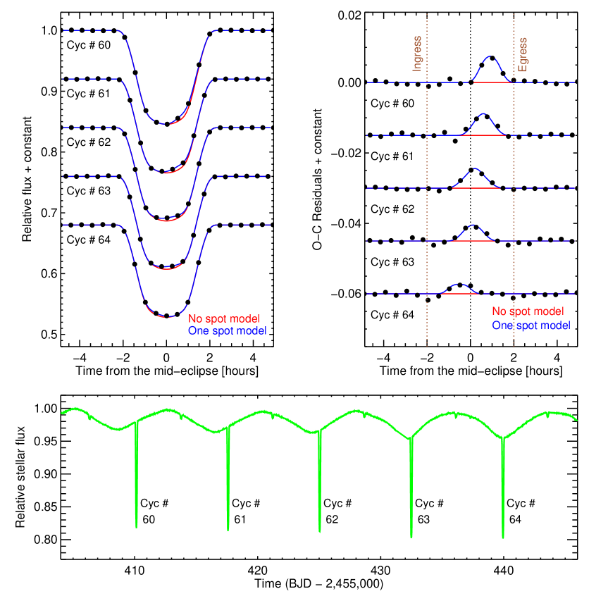
The effect spots have on individual primary eclipses is manifest in two ways: the depth of each eclipse changes since it is measured relative to the changing stellar flux, and the shape of each eclipse is distorted which leads to a shift in the measured mid-eclipse time. Visual inspection of the eclipse residuals shows that this last effect can be well-modeled in most cases by adding just one large star-spot on the surface of the primary star. Since the rotation of the star happens on a longer time-scale than the eclipse itself, we held the position of the star-spot fixed during each individual eclipse. The latitude of the spots cannot be well constrained with single eclipse events, so we fix the position of the spot so that the center of the secondary star trajectory intersects the center of the spot. Our spot model adds five additional parameters: three parameters describe the spot itself – its angular radius, the flux contrast (related to the spot temperature), and the position along the eclipse chord. The fourth parameter is the out-of-eclipse flux, which corrects for the depth variations. Finally, the time of mid-eclipse is free. We set up a pixilated model of the star with a circular spot, in which the flux is calculated as the surface integral of the intensity of the visible hemisphere of the star.
The best-fitting model for several consecutive eclipses is compared with a no-spot model in Fig. S13, showing how the model captures the essential effect of spots on the eclipses. For every eclipse we obtained a new eclipse time, and fitted a linear ephemeris to these times. The scatter was found to be substantially reduced from the initial timings (see Fig. S10, upper panel), by a factor of 30%, which shows that indeed the scatter is due to spots. The improvement on the scatter is similar to the one obtained through the local slope correction, so this serves as a good consistency check.
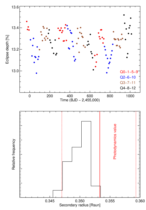
Our model also estimates the fraction of the star covered by spots at the time of each eclipse. This quantity is not very precise, but can help us estimate the effect of spots on the measurement of the eclipse depth and hence the radius ratio . We divide the square of the radius ratio from the spot model by each observed local out-of-eclipse flux to mimic the apparent depth that one would obtain by fitting each eclipse individually. The results are plotted in Fig. S14, where one can clearly see how the depth of each eclipse changes with time. The variations seem to have a time-scale similar to the uncorrected eclipse timing variations, which is expected since the scatter in both are due to spots. A variation with the observing season is also apparent, which is a clear indication that there are different levels of Quarterly contamination. With these eclipse depths we can estimate the inferred secondary star radius from each eclipse, using a fixed from Table 1 (see Fig. S14). The values obtained do not have a large scatter, and they all agree within with the value obtained from the photometric-dynamical model fit. Thus the correction to the secondary star radius because of the presence of spots is not significant, although a slightly smaller radius is favored.
We can also use these spot models to gain information about the obliquity of the system (?, ?, ?, ?, ?). In Fig. S13 we can clearly see how the spot model shows that a spot is moving backwards with each eclipse, which means that the spot trajectory is contained within the boundaries of the eclipse chord. This backwards movement makes it seem as if the star is rotating backwards (retrograde) very slowly, but this is simply a stroboscopic alias effect. The spot appears to move backwards because the star’s rotation period is slightly longer than the orbital period.
If we assume that the entire trajectory of a spot is contained on the part of the primary star eclipsed by the secondary star then we can estimate the obliquity of the system (?) to be smaller than . The obliquity is likely to be smaller since we have detected more than 10 spots receding with different velocities, and these different velocities could be due to spots at different latitudes exhibiting differential rotation. We note that the obliquity of this target will be very hard to measure with the Rossiter-McLaughlin effect (?) due to its faintness, so additional investigation of its spots might be the preferred method to further constrain the obliquity.
In principle, we can use the spectroscopic together with an estimated rotation period and size of the primary star to obtain information on the inclination of the primary star. The spectroscopic observed km s-1, while the inferred km s-1. This would imply a highly inclined star (). Note, however, that the measured value of the rotational velocity is below the resolution of the spectra, so its value should be treated with caution. In addition, differential rotation can make it harder to compare the surface integrated projected rotational velocity to the equatorial rotational velocity (?).
1.8 Transit times for the inner and outer planet and the search for additional transits
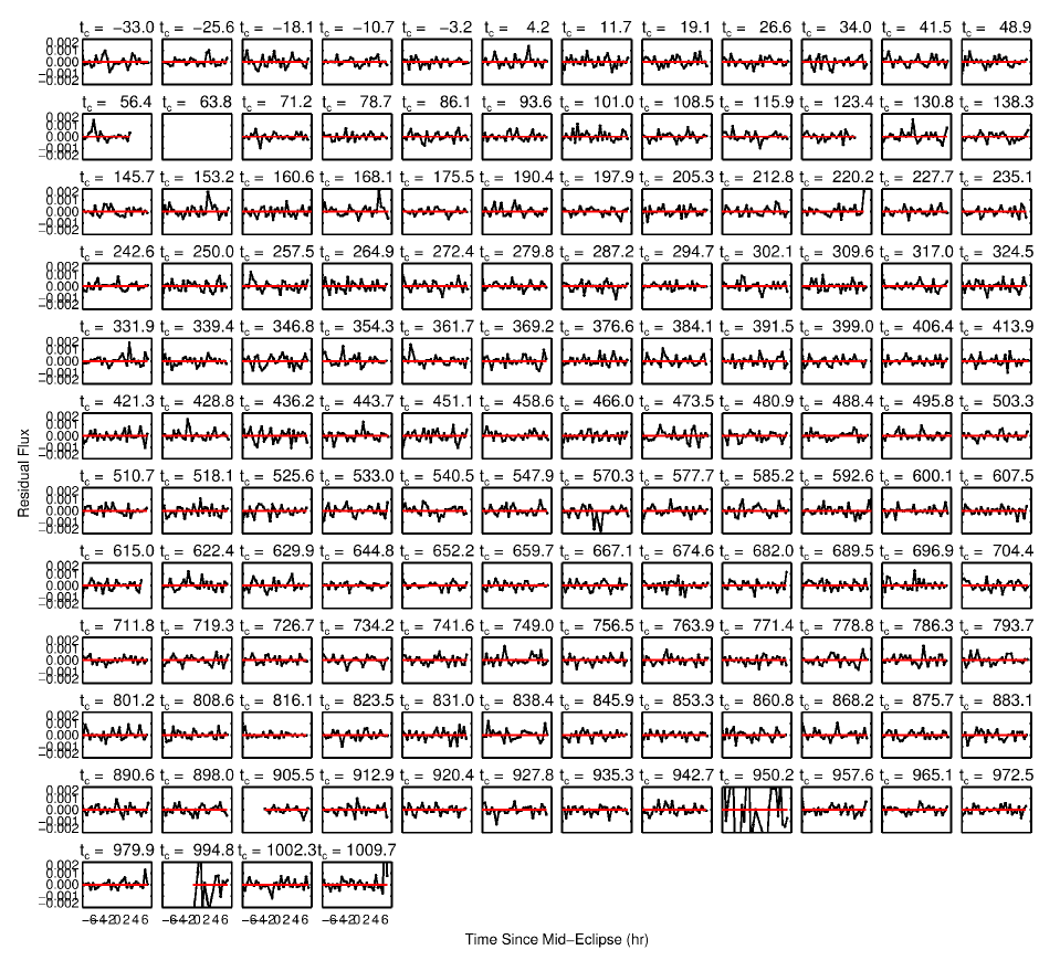
All of the transits of the outer planet and about half of the transits of the inner planet are evident in the SAP light curves before any detrending. The rest became visible when the data are carefully detrended. A symmetric polynomial “U-function” template with an adjustable width and depth was used to estimate the times of mid-transit and their durations. A cubic polynomial was used to detrend each transit using five different duration windows around the transit, and the best-fitting one was adopted. The fits for each transit were iterated to determine the best-fitting time of mid-transit and the duration. This method worked well in some cases and failed to converge in other cases. In cases where the convergence failed, the time was estimated using an interactive plotting program, and an uncertainty of 30, 60 or 90 minutes was assigned based on the judged quality of the transit. Table S4 gives the measured times and durations and their uncertainties, and the corresponding model times and durations. We note that the measured times and the durations were only used to establish starting models for the photometric-dynamical models described below. The actual (detrended) light curve was modeled directly.
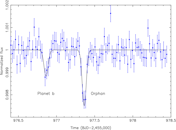
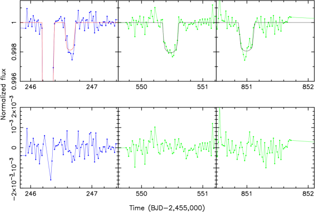
One “orphan” transit occurring about 12 hours after a transit of planet b was noticed in the Q12 data (Fig. S15). This transit cannot be accounted for by either the inner or the outer planet (the intervals between the nearest transits are 0.5 days and 127 days, respectively). To estimate the significance of the orphan event, a model consisting of two Gaussians was fit to the segment of the detrended light curve shown in Fig. S15, which contains 103 data points. The uncertainties on each point were scaled to give for 96 degrees of freedom. The Gaussian in the model at the location of the orphan was replaced by the background level of 1.0 and the resulting value increased to 205.5, giving a formal significance of .
No other orphan transits with a significance of were found using visual searches. An automated search algorithm, dubbed the “Quasi-periodic Automated Transit Search” (QATS) was also used to search for additional transits. The QATS algorithm can allow for unequal time intervals between the transit events. For a given trial period for a potential planet, the expected transit duration at each time in the light curve is computed using a circular orbit for the planet. The data are corrected for the different transit durations and shifted to a common phase to increase the signal-to-noise (the correction for the different widths is quite good, provided the planet’s orbit is nearly circular). A “periodogram” is constructed by plotting the significance versus the trial period. QATS detected the inner planet at high significance. Unfortunately QATS is very sensitive to detrending errors for longer periods, and in fact did not detect the outer planet. No additional planets with periods shorter than 150 days were detected at the significance level of the inner planet.
Although the overall duty cycle of the data collection by Kepler is quite high, a non-trivial amount of the light curve is occupied by the stellar eclipses, which in the case of Kepler-47 is times more than it is for Kepler-16, 34, 35, and 38. Although one could in principle find transits during primary and secondary eclipses, in Kepler-47 this is extremely difficult owing to the effects of star-spots. The primary and secondary eclipse durations together are 0.014 in orbital phase, which is 0.104 days. A combined total of 256 primary and secondary eclipses were observed, giving a total of 26.62 days lost for the purposes of transit searches, lowering the duty cycle to 83.8%.
Finally, if the transit is due to another planet in the Kepler-47 system, its radius would be Earth radii. Without more transit events, it is nearly impossible to determine what the orbital period of such a planet would be. If its orbit is more inclined relative to the other planets, it would not necessarily transit the stars near each conjunction. In addition, if there is precession of the orbit, it is possible for sequences of transits to come and go over long time scales. Thus, the orphan transit could in principle belong to a planet in between the inner and outer one, in spite of the lack of other observed transits.
1.9 Photometric-dynamical model
We modeled the Kepler light curve of Kepler-47 using a dynamical model to predict the motions of the planets and stars, and a eclipse/transit model to predict the light curve.
1.9.1 Description of the model
The “photometric-dynamical model” refers to the model that was used to fit the Kepler photometry. This model is analogous to that described in the analyses of KOI-126 (?), Kepler-16 (?), Kepler-34 and Kepler-35 (?), Kepler-36 (?), and Kepler-38 (?).
Four bodies were involved in this problem; however, the planets’ gravitational interaction with the stars and with each other was determined to be observationally negligible. We therefore assumed the planets to be massless in our model. The motion of the stellar binary was Keplerian and could be predicted analytically. The planets were modeled as orbiting in the two-body potential of the stars. The motion of each planet was determined via a three-body numerical integration. This integration utilized a hierarchical (or Jacobian) coordinate system. In this system, () is the position of Planet b (Planet c) relative to the center-of-mass of the stellar binary (which corresponds to the barycenter in this approximation), and is the position of Star B relative to Star A. The computations are performed in a Cartesian system, although it is convenient to express () and and their time derivatives in terms of osculating Keplerian orbital elements: instantaneous period, eccentricity, argument of pericenter, inclination, longitude of the ascending node, and time of barycentric conjunction: , , , , , , respectively. We note that these parameters do not necessarily reflect observables in the light curve; the unique three-body effects make these parameters functions of time (and we refer to these coordinates as “osculating”).
The accelerations of the three bodies are determined from Newton’s equations of motion, which depend on (), and the masses (?, ?). For the purpose of reporting the masses and radii in Solar units, we assumed AU3 day-2 and AU. We used a Bulirsch-Stoer algorithm (?) to integrate the coupled first-order differential equations for and .
The spatial coordinates of all four bodies at each observed time are calculated and used as inputs to model the light curve. The computed flux was the sum of the fluxes assigned to Star A, Star B, and a seasonal (being the four “seasons” of the Kepler spacecraft orientation) source of “third light,” minus any missing flux due to eclipses or transits (only planetary transits across Star A were computed, those across Star B are not significant in the Kepler data). The loss of light due to eclipses was calculated as follows. All objects were assumed to be spherical. The sum of the fluxes of Star A and Star B was normalized to unity and the flux of Star B was specified relative to that of Star A. The radial brightness profiles of Star A and Star B were modeled with a linear limb-darkening law, i.e., where is the projected distance from the center of a given star, normalized to its radius, and is the linear limb-darkening parameter. The limb darkening coefficient of Star B was fixed (to ); letting it vary freely resulted in a negligible change to final parameter posterior.
The radial velocity of Star A was computed from the time derivative of the position of Star A along the line of sight (analytically, in this case) and compared to the radial velocity data.
The continuous model is integrated over a 29.4 minutes interval centered on each long cadence sample before being compared to the long cadence Kepler data.
1.9.2 Local detrending of Kepler data
The Kepler light curve (“SAP_FLUX” from the standard fits product) for Kepler-47, spanning twelve Quarters, is reduced to only those data within 0.5–1 day of any primary or secondary eclipse or any transit of either planet. As noted above, some data are missing as a result of observation breaks during Quarterly data transfers or spacecraft safe modes.
Each continuous segment of data has a local cubic correction in time divided into it. The parameters of this polynomial correction are found through an iterative process, as described as follows. In the first step, we masked the eclipses of the stars and the transits of the planets and then performed a robust nonlinear least-squares fit to each continuous segment. The data, having divided out this correction, were then “fit” with the photo-dynamical model by determining the highest likelihood solution from a Markov Chain Monte Carlo simulation. The best-fit model was then divided into the data and the local nonlinear fits were recomputed (this time without masking the eclipses and transits). This process was repeated until the corrections converged to a sufficient tolerance.
1.9.3 Specification of parameters
A reference epoch for the three-body integration was specified for each planet near a particular transit. Those epochs were chosen to be 2,454,969.216 BJD and 2,455,246.6545 BJD for planets b and c, respectively.
The model has 33 adjustable parameters. Two parameters are related to Star A: the stellar density times the gravitational constant, , and the stellar mass times , . One parameter gives the mass ratio of the stars, . Six parameters encode the eccentricities and arguments of pericenter for the planetary and stellar orbits about the barycenter in a way that reduces nonlinear correlations:
| (1) | |||||
| (2) | |||||
| (3) | |||||
| (4) |
The remaining osculating parameters, 11 in total, are the periods , , the orbital inclinations , , the times of conjunction with barycenter, , and the difference between the nodal longitudes of the planets to that of the stellar binary . The absolute nodal angle relative to North of the stellar binary cannot be determined and was fixed to zero in practice.
Three more parameters are the relative radii of Star B and the planets to that of Star A: and . One parameter, , parameterizes the linear limb darkening law for Star A (described above). Another parameter gives the relative flux contribution of Star B, .
A single parameter, , describes the width of the probability distribution for the photometric noise of the long cadence observations, assumed to be stationary, white and Gaussian-distributed.
Three parameters characterize the radial velocity measurements: the constant offset of the radial velocity, , the offset between the HET and HJST velocities, , and a “stellar jitter” term, , which contributes to the measured errors for each radial velocity observation, in quadrature. Because only one Keck observation was made, this radial velocity could not be offset to match the HET and HJST velocities in a sensible way, and therefore was omitted in the modeling.
Additionally, we specify 4 more parameters describing the relative extra flux summed in the aperture. The four parameters specify the constant extra flux in each Kepler “season.” The Kepler spacecraft is in one of four orientations during a year; a constant level of “third light” is assumed for all Quarters sharing a common season.
1.9.4 Priors and likelihood
We assumed uniform priors for all 33 parameters. For the eccentricity parameters, this corresponds to uniform priors in and , but a prior that scales as for the stellar eccentricity. This eccentricity is sufficiently determined that this non-uniform prior does not dominate the posterior distribution.
The likelihood of a given set of parameters was taken to be the product of likelihoods based on the photometric data and radial velocity data:
where is the th photometric data residual, is the width parameter describing the photometric noise of the long cadence data, is the th radial velocity residual, is the uncertainty in the th radial velocity measurement and is the stellar jitter term added in quadrature with the .
1.9.5 Best-fit model
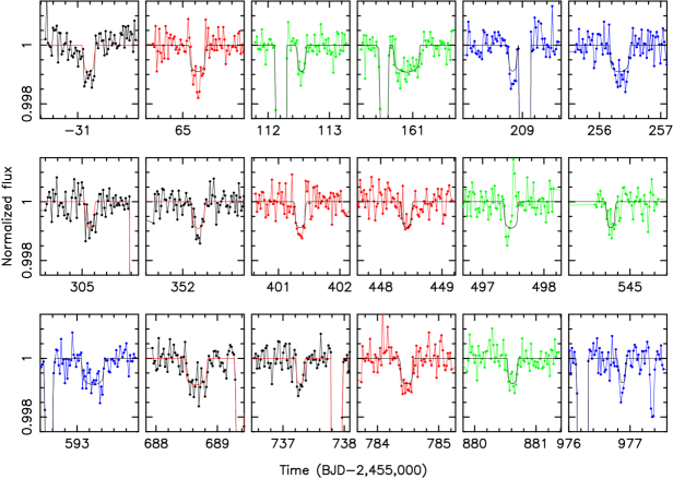
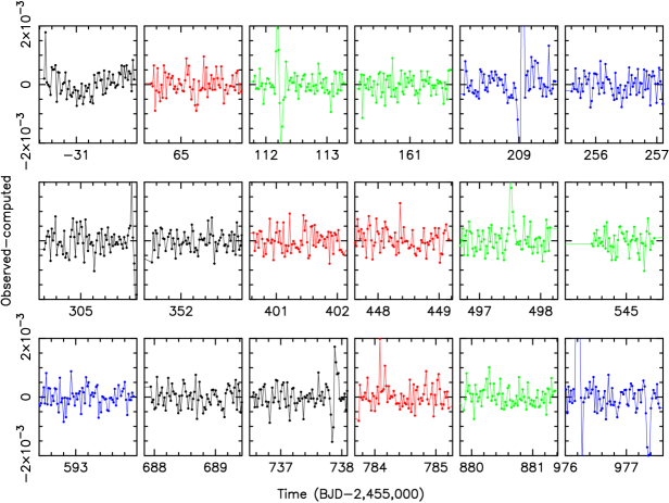
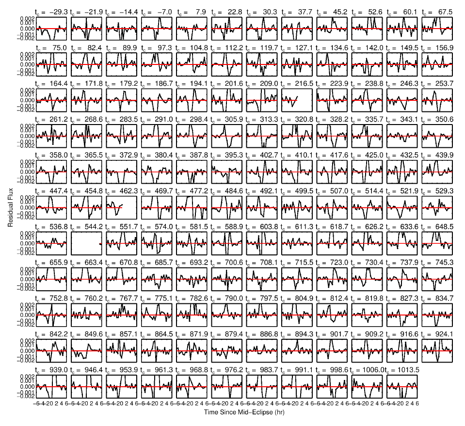
We determined the best-fit model by maximizing the likelihood. The maximum likelihood solution was found by finding the highest likelihood in a large draw from the posterior as simulated with a Markov Chain Monte Carlo simulation as described below. Fig. S16 shows 18 transits of the inner planet, and Fig. S17 shows the residuals (observed data minus the model). With a few exceptions, there are no strong patterns in the residuals. Fig. S18 shows the model fits and the residuals for the outer planet. There are no patterns evident in the residuals. The residuals for the fits to the primary eclipses are shown in Fig. S19 and the residuals for the fits to the secondary eclipses are shown in Fig. S20. Spot crossing events are evident in many of the primary eclipses. Fig. S21 shows the radial velocity measurements and the best-fitting model and the residuals of the fit. Generally the absolute value of the radial velocity residuals is less than about 200 m s-1.
The photometric noise parameter, , has a best-fit value of ppm. For comparison, the root-mean-square deviation of the best-fit residuals is ppm. This is similar to the expected noise in the light curve of 635 ppm as estimated using an on-line tool provided by the Kepler Guest Observer Office111http://keplergo.arc.nasa.gov/CalibrationSN.shtml, where we used an apparent magnitude of Kp=15.18 and 20 pixels in the aperture. For this , the -metric for the photometric data is with 10629 degrees of freedom. If we fail to include planet b in our model (by setting its radius to zero), the increases by . If we ignore planet c, the increases by .
The stellar jitter parameter, , has a best-fit value of km s-1. The value of for the radial velocity data alone is for the 10 radial velocity observations.
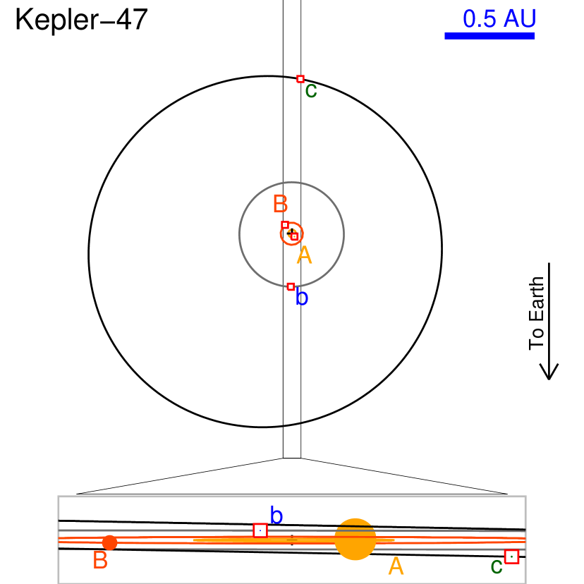
Fig. S22 shows schematic diagrams of the Kepler-47 orbits. The projected orbits of planets b and c cross the projected disk of the primary, and so transits of both planets across the primary occur, as do occultations of both planets by star A. The former events are observed, whereas the latter events are not observable given the noise level. On the other hand, owing to its small radius, the projected disk of star B does not intersect the projected orbits of the planets, and as such no transits of star B or occultations due to star B occur for the best-fitting orbital configuration. Due to the uncertainties in the relative nodal angles, transits of the planets across star B might occur for a subset of the acceptable solutions. However, even if transits across star B did occur, the expected transit depth would be times weaker than the transits across the primary, and would not be observable in the light curve given the noise level.
1.9.6 Parameter estimation methodology
We explored the parameter space and estimated the posterior parameter distribution with a Differential Evolution Markov Chain Monte Carlo (DE-MCMC) algorithm (?).
We generated a population of 100 chains and evolved them through approximately 200,000 generations. The initial parameter states of the 100 chains were randomly selected from an over-dispersed region in parameter space bounding the final posterior distribution. The first 10% of the links in each individual Markov chain were clipped, and the resulting chains were concatenated to form a single Markov chain, after having confirmed that each chain had converged according to the standard criteria.
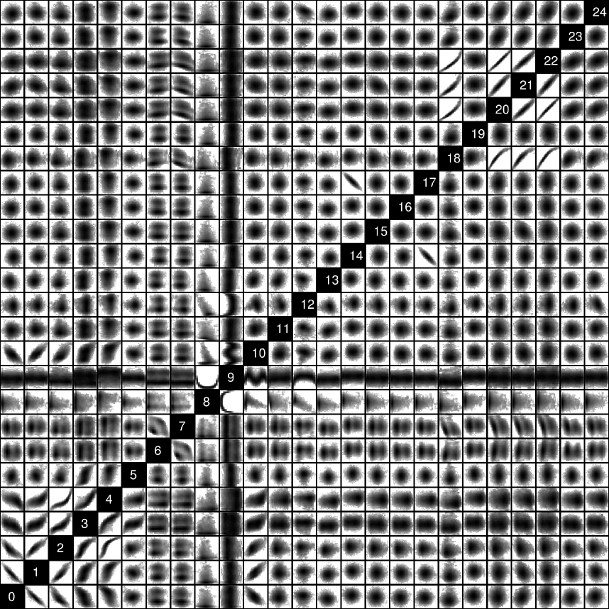
The parameter values and derived values reported in Tables S5 and S6 beside the best-fit values (see above), were found by computing the 15.8%, 50%, 84.2% levels of the cumulative distribution of the marginalized posterior for each parameter. Figure S23 shows two-parameter joint distributions between all parameters. This figure is meant to highlight the qualitative features of the posterior as opposed to providing quantitative ranges. The numbers in that figure correspond to the model parameters in Table S6 with the same number listed as in the first column, if available.
1.9.7 Predicted ephemerides and transit parameters
Tables S7 and S8 provide the predicted times of transit, impact parameters, normalized transit velocities and durations over 7 years, starting with Kepler Quarter Q13.
1.10 ELC light curve models
Although the secondary star is not detected spectroscopically, its temperature can be estimated using the temperature of the primary derived using SPC, and the temperature ratio derived from modeling the eclipses. In order to find the temperature ratio, and to have an independent check on the results from the photometric-dynamical model, we modeled the light and velocity curves using the Eclipsing Light Curve (ELC) code (?) with its genetic algorithm and Monte Carlo Markov Chain optimizers. The free parameters include the temperature ratio , the primary’s limb darkening parameters and for the quadratic limb darkening law [], the orbital parameters (, , ), and the fractional radii and . The stellar masses and the orbital period were held fixed at the values derived from the photometric-dynamical model discussed above.
In ELC, the shapes of the stars are computed using a “Roche” potential modified to account for nonsynchronous rotation and eccentric orbits (?, ?). Given the mass ratio and the fractional radii, the volumes of each star are found by numerical integration. The effective radius of each star is taken to be the radius of a sphere with the same volume as the equipotential surface. In the case of Kepler-47, the stars are very nearly spherical. For the primary at periastron, the ratio of the polar radius to its effective radius is 0.99988, and the ratio of the radius along the line of centers to the effective radius is 1.00007. The amplitude of the out-of-eclipse modulation in the light curve due to ellipsoidal variations, reflection, and Doppler boosting is on the order of 400 ppm, which is times smaller than the modulation due to star-spots. Thus the use of spherical stars in the photometric-dynamical model is a very good approximation.
Since the numerical integrations are very CPU intensive, ELC has a fast “analytic” mode where the equations given in (?) are used. The normalized light curve was divided into 41 segments containing two or three pairs of primary and secondary eclipses. These segments were modeled separately in order to help assess the systematic errors associated with the changing star-spots and the changes in the contamination from Quarter to Quarter. For each fitting parameter, we computed the mean of the best-fitting values and the standard deviation. Table S10 gives the mean values and standard deviations, which we adopt as errors.
Based on the temperature of the primary derived from the SPC analysis, and the temperature ratio found from the ELC models, we derive a temperature of K for the secondary.
1.11 Upper limits on planetary masses
Upper limits on the masses of the planets can be placed separately as follows. The mass of the inner planet is best constrained by the lack of eclipse timing variations due to gravitational perturbations from that planet. The planet will induce short-term eclipse timing variations with a period equal to the planet’s period. It will also cause precession of the binary. Over the time-scale of a few years, the binary precession will cause a slight change in the phase difference between the primary and secondary eclipses, which can be observed as a slight difference between the primary and secondary eclipse periods. Numerical simulations showed that in this case the stronger upper limit comes from the lack of short-term eclipse timing variations. A grid of masses for the inner planet was used, and equations of motion for a three body system were integrated, holding the orbital parameters of the binary at their best-fitting values (the nature of the perturbations on the binary are insensitive to anything except the planet’s mass). The period and epoch of the binary was found, and the predicted times of eclipse were compared to the measured times. The value changes smoothly with the planet’s mass, and going to gives a upper limit of 2.7 Jupiter masses for the uncorrected eclipse times and 2.0 Jupiter masses for the eclipse times corrected for the effect of star-spots. We adopt the latter value as the upper limit on the mass of the inner planet.
The mass of the outer planet was best constrained by light travel time (LTT) effects. We fit an LTT orbit to the corrected eclipse times, using a period of 303.13 days and constraining the eccentricity to be . While no convincing signal is seen at that period, the best-fitting orbit formally has a semiamplitude of seconds. Given the total mass of the binary and the period of the outer planet, we find a upper mass limit of 28 Jupiter masses.
1.12 Stability of orbits and limits on eccentricity
We carried out an extensive study of the dynamics of the system and its long-term stability. The orbits of the two planets were integrated, numerically, for different values of their masses and orbital eccentricities. To determine an upper limit for the eccentricity of planet c, we held constant all orbital elements at their best-fit values and integrated the system varying the eccentricity of this planet. Results indicated that the system maintained stability for at least 100 Myr and for . An examination of the semimajor axis, eccentricity, and orbital inclination of each planet during the course of the integrations showed that the variations of these quantities were negligibly small, supporting the idea that the two planets do not disturb each other’s orbits. The results stayed unchanged when the masses of the two planets were increased to 0.21 and 0.63 Jupiter masses, roughly ten times their plausible values based on the empirical mass-radius relations (?, ?).
Both the photometric-dynamical model and stability simulations used a Newtonian 4-body numerical integrator. A more physical model would include the precession of the binary due to general relativity (GR) and the tidal and rotational bulges. Expressions for the rate of precession due to these effects (?) show that GR dominates, and it would cause a full periastron rotation in years. In the current observations, such precession would cause the period of primary and secondary eclipse to differ fractionally by , whereas the uncertainty of this quantity is . The GR precession period is much longer than the periastron period of the planets – e.g., numerical integrations of planet c showing a year precession cycle due to the effective quadrupolar gravitational potential of the binary – so it has little dynamical importance. Therefore GR and other precession effects are neither detectable nor significantly change our assessment of stability, so GR has little dynamical importance.
1.13 Comparison with stellar evolution models
The reasonably precise absolute dimensions determined for the stars in Kepler-47 (4–5% relative errors for the masses, and 1.8% for the radii) offer an opportunity to compare the measurements with models of stellar evolution. This is of particular interest for the late M-dwarf secondary, given that low-mass stars have shown discrepancies with theory in the sense that they are generally larger and cooler than predicted. These anomalies are believed to be due to stellar activity (?, ?).
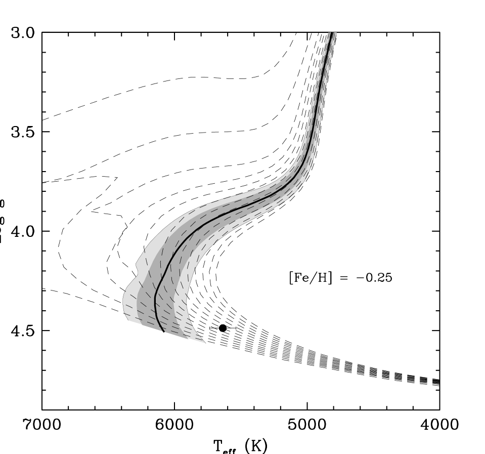
In Fig. S27 we compare the measurements for the primary star with a stellar evolution track from the Yonsei-Yale series (?, ?), interpolated to the exact mass we measure. The metallicity of this model is set by our spectroscopic determination of , where we assume the iron abundance tracks the metallicity measurement from SPC. The model is consistent with the observations to within less than , and the small difference may be due either to slightly biased spectroscopic parameters (temperature and metallicity) or a slightly overestimated mass for the primary star. As a check, we produced a photometric estimate of the temperature using available photometry from the KIC and empirical color-temperature calibrations along with the reddening listed in the KIC. The result suggests a value closer to 5900 K than 5600 K, although we consider this evidence to be somewhat circumstantial and highly dependent on reddening. We confirmed that the level of agreement between theory and observation is independent of the adopted model physics by comparing the primary star parameters with BaSTI stellar evolutionary tracks (?), which yielded similar results as the Yonsei-Yale models.
In Fig. S28 we compare the measurements for both components against models from the Dartmouth series (?), which incorporate physical ingredients (equation of state, non-grey boundary conditions) more appropriate for low-mass stars. We find the radius of the secondary of Kepler-47 to be consistent with these models, which would be an exception to the general trend mentioned above, although the mass error is large enough (4%) that the conclusion is not as strong as in other cases. Its temperature, however, is lower than predicted for a star of this mass by about 200 K. This deviation is in the same direction as seen for other low-mass stars. Because the secondary is so faint, we have no information on its activity level. Age estimates for the system from this figure and the previous one are somewhat conflicting, and only allow us to say that Kepler-47 is very roughly of solar age.
1.14 Details of habitable zone
To determine the insolation limits of the habitable zone for Kepler-47 c, we follow the relations given by (?) that include the stellar temperature as well as luminosity. The temperature term accounts for the different relative amount of infrared flux to total flux, which is important for atmospheric heating. We use the criteria of a runaway greenhouse effect for the inner boundary and the maximum greenhouse effect for a cloud-free carbon dioxide atmosphere for the outer boundary. This is more conservative than the “recent Venus” and “early Mars” criteria, but less conservative than the “water loss” and “first carbon dioxide condensation” criteria (?). The secondary star emits only 1.7% as much energy as the primary star (and only 0.58% in the Kepler bandpass), so its contribution is neglected. The resulting insolation limits are shown as the dotted lines in Figure 3 (main text). The relations given in (?), i.e. a cloud-free atmosphere yield nearly identical limits.
The average insolation for Kepler-47 c for a circular orbit is 87% of the Sun-Earth insolation, and varies by peak-to-peak. For an eccentricity of 0.2 the mean insolation is 89% and varies from 59% to 144% of the Sun-Earth value; for an eccentricity of 0.4, the mean is 96% and varies from 43% to 261%. Even in this latter case, which is ruled out at the 95% confidence level by the photometric-dynamical model, the mean is less than the Sun-Earth value, and it is the mean insolation that is most relevant for habitability (?). Thus for all allowed eccentricities, Kepler-47 c lies in the habitable zone.
Because the primary star dominates the system both in luminosity and mass (so the primary star remains near the barycenter), the variation in insolation is relatively small for a circular planetary orbit. This is seen in the upper left panel of Figure 3, where the variations are caused by the 7.4-day orbit of the primary star. For large eccentricities, the variation in insolation are dominated by the non-circular orbit of the planet.
It must be stressed that the habitable zone is defined such that liquid water could persist for a biologically significant time period on an Earth-like planet (i.e. with a terrestrial CO2/H2O/N2 atmosphere, plate tectonics, etc.), and the formulations of (?, ?, ?) explicitly assume such conditions. For Kepler-47 c these conditions are not met. Nevertheless, the main point is that Kepler-47 c receives approximately the same amount of energy from its stars that the Earth receives from the Sun.
While it neglects most atmospheric physics, the equilibrium temperature of the planet is still a useful characterization. Assuming that the entire surface of the planet radiates isothermally (i.e. the stellar insolation is efficiently advected around the planet), and for a Bond albedo of =0.7, appropriate for a Neptune-size planet and 1 Sun-Earth insolation (?), a value of is found for eccentricities from 0.0 to 0.3. For =0.34, corresponding to the albedos of Jupiter and Saturn, . For an Earth-like albedo of 0.29, which is appropriate for a habitable-zone planet, . The greenhouse effect will lead to temperatures at the 1-bar pressure level that are higher by several tens of degrees.
References and Notes
- 1. D. G. Koch, W. J. Borucki, G. Basri, N. M. Batalha, T. M. Brown, et al., Kepler mission design, realized photometric performance, and early science. Astrophys. J. 713, L79-L86 (2010).
- 2. W. J. Borucki, D. Koch, G. Basri, N. Batalha, T. Brown, et al., Kepler Planet-Detection Mission: Introduction and First Results. Science 327, 977-980 (2010).
- 3. N. M. Batalha, J. F. Rowe, S. T. Bryson, T. Barclay, C. J. Burke, et al., Planetary candidates observed by Kepler, III: analysis of the first 16 months of data. Astrophys. J. Suppl. Ser. submitted, arXiv:1202.5852, (2012).
- 4. A. Prša, A., N. Batalha, R. W. Slawson, L. R. Doyle, W. F. Welsh, et al., Kepler eclipsing binary stars. I. catalog and principal characterization of 1879 eclipsing binaries in the first data release. Astron. J. 141, 83 (2011).
- 5. R. W. Slawson, A. Prša, W. F. Welsh, J. A. Orosz, M. Rucker, et al., Kepler eclipsing binary stars. II. 2165 eclipsing binaries in the second data release. Astron. J. 142, 160 (2011).
- 6. L. R. Doyle, J. A. Carter, D. C. Fabrycky, R. W. Slawson, S. B. Howell, et al., Kepler-16: a transiting circumbinary planet. Science 333, 1602-1606 (2011).
- 7. W. F. Welsh, J. A. Orosz, J. A. Carter, D. C. Fabrycky, E. B. Ford, et al., Transiting circumbinary planets Kepler-34 b and Kepler-35 b. Nature 481, 475-479 (2012).
- 8. J. A. Orosz, W. F. Welsh, J. A. Carter, E. Brugamyer, L. A., Buchhave, et al., The Neptune-sized circumbinary planet Kepler-38b. Astrophys. J. in press, arXiv:1208.3712 (2012).
- 9. S. Meschiari, Circumbinary planet formation in the Kepler-16 system. I. N-body simulations. Astrophys. J. 752, 71 (2012).
- 10. S.-J. Paardekooper, Z. M. Leinhardt, P. Thébault, & C. Baruteau, How not to build Tatooine: the difficulty of in situ formation of circumbinary planets Kepler 16b, Kepler 34b, and Kepler 35b. Astrophys. J. 754, L16 (2012).
- 11. T. Borkovits, B. Érdi, E. Forgács-Dajka, & T. Kovács, On the detectability of long period perturbations in close hierarchical triple stellar systems. Astron. Astroph. 398, 1091-1102 (2003).
- 12. See the Supplementary Materials on Science Online.
- 13. J. A. Carter, D. C. Fabrycky, D. Ragozzine, M. J. Holman, S. N. Quinn, et al., KOI-126: A triply eclipsing hierarchical triple with two low-mass stars. Science 331, 562-565 (2011).
- 14. S. R. Kane, & D. M. Gelino, The habitable zone gallery. Pubs. Astron. Soc. Pac. 124, 323-328 (2012).
- 15. J. J. Lissauer, D. Ragozzine, D. C. Fabrycky, J. H. Steffen, E. B. Ford, et al., Architecture and dynamics of Kepler’s candidate multiple transiting planet systems. Astrophys. J. Suppl. Ser. 197, 8 (2011).
- 16. M. J. Holman, & P. A. Wiegert, Long-term stability of planets in binary systems. Astron. J. 117, 621-628 (1999).
- 17. J. F. Kasting, D. P. Whitmire, & R. T. Reynolds, Habitable zones around main sequence stars. Icarus 101, 108-128 (1993).
- 18. R. Sanchis-Ojeda, J. N. Winn, M. J. Holman, J. A. Carter, D. J. Osip, & C. I. Fuentes, Starspots and spin-orbit alignment in the WASP-4 exoplanetary system. Astrophys. J. 733, 127 (2011).
- 19. P. A. Nutzman, D. C. Fabrycky, & J. J. Fortney, Using star spots to measure the spin-orbit alignment of transiting planets. Astrophys. J. 740, L10 (2011).
- 20. J. M. Désert, D. Charbonneau, B.-O. Demory, S. Ballard, J. A. Carter, et al., The Hot-Jupiter Kepler-17b: discovery, obliquity from stroboscopic starspots, and atmospheric characterization. et al., Astrophys. J. Suppl. Ser. 197, 14 (2011).
- 21. R. Sanchis-Ojeda, D. C. Fabrycky, J. N. Winn, T. Barclay, B. D. Clarke, et al., Alignment of the stellar spin with the orbits of a three-planet system. Nature 487, 449-453 (2012).
- 22. A. Pierens, & R. P. Nelson, On the formation and migration of giant planets in circumbinary discs. Astron. Astroph. 483, 633-642 (2008).
- 23. A. N. Youdin, K. M. Krautter, & S. J. Kenyon, Circumbinary Chaos: Using Pluto’s Newest Moon to Constrain the Masses of Nix and Hydra. Astrophys. J. 755, 17 (2012).
- 24. D. R. Underwood, B. W. Jones, & P. N. Sleep, The evolution of habitable zones during stellar lifetimes and its implications on the search for extraterrestrial life. Int. J. Ast. Bio. 2, 289-299 (2003).
- 25. T. M. Brown, D. W. Latham, M. E. Everett, & G. A. Esquerdo, Kepler input catalog: photometric calibration and stellar classification. Astron. J. 142, 112 (2011)
- 26. K. Kinemuchi, T. Barclay, M. Fanelli, J. Pepper, M. Still, & S. B. Howell, Demystifying Kepler data: a primer for systematic artifact mitigation. Publ. Astron. Soc. Pac. in press, arXiv:1207.3093, (2012).
- 27. T. Mazeh, in Observational Evidence for Tidal Interaction in Close Binary Systems, eds. M.-J. Goupil & J.-P. Zahn, EAS Publications Series, vol. 29, p. 29 (2008).
- 28. R. G. Tull, High-resolution fiber-coupled spectrograph of the Hobby-Eberly Telescope. Proc. Soc. Photo-opt. Inst. Eng. 3355, 387-398 (1998).
- 29. R. G. Tull, P. J. MacQueen, C. Sneden, C. & D. L. Lambert, The high-resolution cross-dispersed echelle white-pupil spectrometer of the McDonald Observatory 2.7-m telescope. Publ. Astron. Soc. Pacif. 107, 251-264 (1995).
- 30. S. S. Vogt, S. L. Allen, B. C. Bigelow, L. Bresee, B. Brown, et al., HIRES: the high-resolution echelle spectrometer on the Keck 10-m Telescope. Proc. Soc. Photo-opt. Inst. Eng. 2198, 362 (1994).
- 31. G. W. Marcy, R. P. Butler, S. S. Vogt, D. A. Fischer, J. T. Wright, et al., Exoplanet properties from Lick, Keck and AAT. Physica Scripta Volume T 130, 014001 (2008).
- 32. S. M. Rucinski, Spectral-line broadening functions of WUMa-type binaries. I - AW UMa. AJ 104, 1968-1981 (1992).
- 33. D. L. Nidever, G. W. Marcy, R. P. Butler, D. A. Fischer, & S. S. Vogt, Radial velocities for 889 late-type stars. Astrophys. J. Suppl. Ser. 141, 502-522 (2002).
- 34. C. Chubak, G. W. Marcy, D. A. Fischer, A. W. Howard, H. Isaacson, H., et al., Precise radial velocities of 2046 nearby FGKM stars and 131 standards. Astrophys. J. Supp. Ser. submitted, arXiv:1207.6212v1, (2012).
- 35. L A. Buchhave, D. W. Latham, A. Johansen, M. Bizzarro, G. Torres, et al., An abundance of small exoplanets around stars with a wide range of metallicities. Nature 486, 375-377 (2012).
- 36. S. Czesla, K. F. Huber, U. Wolter, S. Schröter, J. H. M. M. Schmitt, How stellar activity affects the size estimates of extrasolar planets. Astron. Astroph. 505, 1277-1282 (2009).
- 37. J. A. Carter, J. N. Winn, M. J. Holman, D. C. Fabrycky, Z. K. Berta, et al., The transit light curve project. XIII. sixteen transits of the Super-Earth GJ 1214b. Astrophys. J. 730, 82 (2011).
- 38. K. Mandel, & E. Agol, Analytic light curves for planetary transit searches. Astrophys. J. 580, L171-L175 (2002).
- 39. T. Hirano, R. Sanchis-Ojeda, Y. Takeda, N. Narita, J. N. Winn, et al. Measurements of stellar inclinations for Kepler planet candidates. Astrophys. J. in press, arXiv:1205.3233, (2012).
- 40. J. N. Winn, R. W. Noyes, M. J. Holman, D. Charbonneau, Y. Oha, et al. Measurement of spin-orbit alignment in an extrasolar planetary system. Astrophys. J. 631, 1215-1226 (2005).
- 41. J. A. Carter, E. Agol, W. J. Chaplin, S. Basu, T. R. Bedding, et al., Kepler-36: a pair of planets with neighboring orbits and dissimilar densities. Science 337, 556-559 (2012).
- 42. S. Soderhjelm, Third-order and tidal effects in the stellar three-body problem. Astron. Astrophy. 141, 232–240 (1984).
- 43. R. A. Mardling, & D. N. C. Lin, Calculating the tidal, spin, and dynamical evolution of extrasolar planetary systems. The Astroph. J. 573, 829–844 (2002).
- 44. W. H. Press, S. A. Teukolsky, W. T. Vetterling, & B. P. Flannery, Numerical recipes in C++ : the art of scientific computing. (Cambridge University Press, Cambridge, 2002).
- 45. C. J. F. ter Braak, & J. A. Vrugt, J.A., A Markov Chain Monte Carlo version of the genetic algorithm Differential Evolution: easy Bayesian computing for real parameter spaces. Statistics and Computing 16, 239–249 (2006).
- 46. J. A. Orosz, & P. H. Hauschildt, The use of the NextGen model atmospheres for cool giants in a light curve synthesis code. Astron. Astrophys. 364, 265-281 (2000).
- 47. Y. Avni, The eclipse duration of the X-ray pulsar 3U 0900-40. Astrophys. J. 209, 574-577 (1976).
- 48. R. E. Wilson, Eccentric orbit generalization and simultaneous solution of binary star light and velocity curves. Astrophys. J. 234, 1054-1066 (1979).
- 49. A. Giménez, Equations for the analysis of the light curves of extra-solar planetary transits. Astron. Astrophys. 450, 1231-1237 (2006).
- 50. D. Fabrycky, Non-Keplerian dynamics of exoplanets. in Exoplanets. ed. S. Seager, University of Arizona Press, p. 217 (2011).
- 51. M. López-Morales, On the correlation between the magnetic activity levels, metallicities, and radii of low-mass stars. Astrophys. J. 660, 732-739 (2007).
- 52. G. Torres, J. Andersen, & A. Giménez, Accurate masses and radii of normal stars: modern results and applications. Astron. & Astrophys. Rev 18, 67-126 (2010).
- 53. S. Yi, P. Demarque, Y. -C. Kim, Y. -W. Lee, C. H. Ree, T. Lejeune, & S. Barnes, Toward better age estimates for stellar populations: the Y2 isochrones for solar mixture. Astrophys. J. Suppl. Ser. 136, 417-437 (2001).
- 54. P. Demarque, J. H. Woo, Y. -C. Kim, & S. K. Yi, Y2 Isochrones with an improved core overshoot treatment. Astrophys J. Suppl. Ser. 155, 667-674 (2004).
- 55. A. Pietrinferni, S. Cassisi, M. Salaris, & F. Castelli, A large stellar evolution database for population synthesis studies. I. scaled solar models and isochrones. Astrophys. J. 612, 168-190 (2004).
- 56. A. Dotter, B. Chaboyer, D. Jevremović, V. Kostov, E. Baron, & J. W. Ferguson, The Dartmouth stellar evolution database. Astrophys. J. Suppl. Ser. 178, 89-101 (2008).
- 57. F. Selsis, J. F. Kasting, B. Levrad, J. Paillet, I. Ribas, & X. Defosse, Habitable planets around the star Gliese 581?. Astron. Astroph. 475, 1373-1387 (2007).
- 58. D. M. Williams, & D. Pollard, Earth-like worlds on eccentric orbits: excursions beyond the habitable zone. Int. J. Ast. Bio. 1, 61-69 (2002).
- 59. K. L. Cahoy, M. S. Marley, & J. J. Fortney, Exoplanet albedo spectra and colors as a function of planet phase, separation, and metallicity. Astrophys. J. 724, 189-214 (2010).





| Date | UT Time | BJD | RVA | telescope |
|---|---|---|---|---|
| YYYY-MM-DD | (2,455,000+) | km s-1 | ||
| 2012-04-10 | 13:25:48.68 | 1028.05942 | Keck | |
| 2012-04-23 | 09:11:27.36 | 1040.90325 | HET | |
| 2012-05-01 | 09:52:55.08 | 1048.93237 | HJST | |
| 2012-05-02 | 07:23:45.95 | 1049.82882 | HJST | |
| 2012-05-04 | 08:34:10.40 | 1051.88474 | HJST | |
| 2012-05-05 | 08:08:26.83 | 1052.86692 | HJST | |
| 2012-05-06 | 08:08:55.42 | 1053.86729 | HJST | |
| 2012-05-18 | 07:35:21.15 | 1065.83749 | HET | |
| 2012-05-20 | 07:37:07.78 | 1067.83880 | HET | |
| 2012-06-05 | 06:29:24.15 | 1083.79236 | HET | |
| 2012-06-26 | 08:03:52.39 | 1104.85862 | HJST |
| parameter | value |
|---|---|
| (K) | |
| (cgs dex) | |
| m/H (dex) | |
| (km s-1) |
| cycle # | primary | corrected | uncertainty | cycle # | secondary | uncertainty |
|---|---|---|---|---|---|---|
| time222BJD-2,455,000 | time1 | (min) | time1 | (min) | ||
| 0.0 | … | … | … | 0.4873910 | -33.12216 | 2.18 |
| 1.0 | -29.30630 | -29.30631 | 0.39 | 1.4873910 | -25.67634 | 2.58 |
| 2.0 | -21.85791 | -21.85777 | 0.37 | 2.4873910 | -18.23125 | 2.18 |
| 3.0 | -14.40955 | -14.40931 | 0.42 | 3.4873910 | -10.78077 | 2.18 |
| 4.0 | -6.96153 | -6.96144 | 0.43 | 4.4873910 | -3.33057 | 2.18 |
| 5.0 | … | … | … | 5.4873910 | 4.11649 | 2.18 |
| 6.0 | 7.93529 | 7.93560 | 0.34 | 6.4873910 | 11.56631 | 2.48 |
| 7.0 | … | … | … | 7.4873910 | 19.01194 | 2.28 |
| 8.0 | 22.83203 | 22.83220 | 0.34 | 8.4873910 | 26.46447 | 2.38 |
| 9.0 | 30.28050 | 30.28080 | 0.33 | 9.4873910 | 33.91396 | 2.08 |
| 10.0 | 37.72889 | 37.72909 | 0.32 | 10.4873910 | 41.36049 | 2.28 |
| 11.0 | 45.17721 | 45.17755 | 0.33 | 11.4873910 | 48.80785 | 2.18 |
| 12.0 | 52.62549 | 52.62570 | 0.35 | 12.4873910 | … | … |
| 13.0 | 60.07424 | 60.07443 | 0.35 | 13.4873910 | … | … |
| 14.0 | 67.52268 | 67.52276 | 0.44 | 14.4873910 | 71.15005 | 2.18 |
| 15.0 | 74.97091 | 74.97090 | 0.41 | 15.4873910 | 78.60117 | 2.38 |
| 16.0 | 82.41951 | 82.41949 | 0.39 | 16.4873910 | 86.04829 | 2.18 |
| 17.0 | 89.86795 | 89.86809 | 0.39 | 17.4873910 | 93.49997 | 2.18 |
| 18.0 | 97.31647 | 97.31640 | 0.27 | 18.4873910 | 100.94826 | 2.38 |
| 19.0 | 104.76482 | 104.76476 | 0.29 | 19.4873910 | 108.39407 | 2.18 |
| 20.0 | 112.21316 | 112.21285 | 0.37 | 20.4873910 | 115.84301 | 2.18 |
| 21.0 | 119.66158 | 119.66138 | 0.28 | 21.4873910 | 123.29027 | 2.28 |
| 22.0 | 127.10971 | 127.10951 | 0.24 | 22.4873910 | 130.73599 | 2.18 |
| 23.0 | 134.55816 | 134.55805 | 0.38 | 23.4873910 | 138.18757 | 2.28 |
| 24.0 | 142.00644 | 142.00639 | 0.32 | 24.4873910 | 145.63522 | 2.38 |
| 25.0 | 149.45473 | 149.45475 | 0.32 | 25.4873910 | 153.08287 | 2.28 |
| 26.0 | … | … | … | 26.4873910 | 160.53488 | 2.48 |
| 27.0 | 164.35156 | 164.35158 | 0.30 | 27.4873910 | 167.98079 | 2.08 |
| 28.0 | 171.80006 | 171.80016 | 0.34 | 28.4873910 | 175.43139 | 2.18 |
| 29.0 | 179.24807 | 179.24806 | 0.25 | 29.4873910 | … | … |
| 30.0 | 186.69626 | 186.69604 | 0.33 | 30.4873910 | 190.32626 | 2.18 |
| 31.0 | 194.14450 | 194.14486 | 0.33 | 31.4873910 | 197.77523 | 2.28 |
| 32.0 | 201.59277 | 201.59307 | 0.40 | 32.4873910 | 205.22572 | 2.18 |
| 33.0 | 209.04129 | 209.04161 | 0.48 | 33.4873910 | 212.67172 | 2.18 |
| 34.0 | … | … | … | 34.4873910 | 220.11933 | 2.18 |
| 35.0 | 223.93826 | 223.93843 | 0.41 | 35.4873910 | 227.56783 | 2.28 |
| 36.0 | … | … | … | 36.4873910 | 235.01738 | 2.18 |
| 37.0 | 238.83553 | 238.83546 | 0.31 | 37.4873910 | 242.46451 | 2.18 |
| 38.0 | 246.28389 | 246.28401 | 0.33 | 38.4873910 | 249.91181 | 2.18 |
| 39.0 | 253.73230 | 253.73247 | 0.29 | 39.4873910 | 257.36186 | 2.58 |
| 40.0 | 261.18019 | 261.18031 | 0.25 | 40.4873910 | 264.80933 | 2.18 |
| 41.0 | 268.62872 | 268.62889 | 0.27 | 41.4873910 | 272.25848 | 2.18 |
| 42.0 | … | … | … | 42.4873910 | 279.70576 | 2.18 |
| 43.0 | 283.52551 | 283.52545 | 0.33 | 43.4873910 | 287.15579 | 2.58 |
| 44.0 | 290.97418 | 290.97397 | 0.32 | 44.4873910 | 294.60501 | 2.18 |
| 45.0 | 298.42259 | 298.42234 | 0.38 | 45.4873910 | 302.05267 | 2.18 |
| 46.0 | 305.87113 | 305.87077 | 0.28 | 46.4873910 | … | … |
| 47.0 | 313.31965 | 313.31911 | 0.33 | 47.4873910 | 316.94980 | 2.18 |
| 48.0 | 320.76803 | 320.76741 | 0.31 | 48.4873910 | 324.39888 | 2.18 |
| 49.0 | 328.21635 | 328.21580 | 0.33 | 49.4873910 | 331.84676 | 2.08 |
| 50.0 | 335.66454 | 335.66432 | 0.30 | 50.4873910 | 339.29309 | 2.28 |
| 51.0 | 343.11269 | 343.11255 | 0.27 | 51.4873910 | 346.74032 | 2.18 |
| 52.0 | 350.56108 | 350.56100 | 0.37 | 52.4873910 | 354.18991 | 2.28 |
| 53.0 | 358.00916 | 358.00920 | 0.37 | 53.4873910 | 361.63907 | 2.18 |
| 54.0 | 365.45750 | 365.45727 | 0.35 | 54.4873910 | 369.08855 | 2.18 |
| 55.0 | 372.90583 | 372.90553 | 0.37 | 55.4873910 | 376.53673 | 2.38 |
| 56.0 | 380.35414 | 380.35434 | 0.34 | 56.4873910 | 383.98453 | 2.38 |
| 57.0 | 387.80274 | 387.80304 | 0.29 | 57.4873910 | 391.43301 | 2.38 |
| 58.0 | 395.25105 | 395.25158 | 0.28 | 58.4873910 | 398.88193 | 2.28 |
| 59.0 | 402.69932 | 402.69981 | 0.39 | 59.4873910 | 406.33048 | 2.28 |
| 60.0 | 410.14753 | 410.14797 | 0.39 | 60.4873910 | 413.77876 | 2.48 |
| 61.0 | 417.59598 | 417.59649 | 0.37 | 61.4873910 | 421.22705 | 2.28 |
| 62.0 | 425.04448 | 425.04486 | 0.41 | 62.4873910 | 428.67664 | 2.18 |
| 63.0 | 432.49299 | 432.49335 | 0.39 | 63.4873910 | 436.12677 | 2.48 |
| 64.0 | 439.94160 | 439.94159 | 0.38 | 64.4873910 | 443.57389 | 2.28 |
| 65.0 | 447.38994 | 447.38962 | 0.41 | 65.4873910 | 451.01777 | 2.28 |
| 66.0 | 454.83858 | 454.83824 | 0.42 | 66.4873910 | 458.46973 | 2.28 |
| 67.0 | … | … | … | 67.4873910 | 465.91872 | 2.18 |
| 68.0 | 469.73590 | 469.73511 | 0.49 | 68.4873910 | 473.36673 | 2.18 |
| 69.0 | 477.18426 | 477.18334 | 0.43 | 69.4873910 | 480.80983 | 2.18 |
| 70.0 | 484.63273 | 484.63184 | 0.42 | 70.4873910 | 488.26371 | 2.18 |
| 71.0 | 492.08030 | 492.07982 | 0.29 | 71.4873910 | 495.71273 | 2.08 |
| 72.0 | 499.52841 | 499.52831 | 0.35 | 72.4873910 | 503.15841 | 2.28 |
| 73.0 | 506.97666 | 506.97688 | 0.37 | 73.4873910 | 510.60646 | 2.28 |
| 74.0 | 514.42490 | 514.42526 | 0.33 | 74.4873910 | 518.05528 | 2.18 |
| 75.0 | 521.87334 | 521.87356 | 0.31 | 75.4873910 | 525.50508 | 2.28 |
| 76.0 | 529.32182 | 529.32216 | 0.28 | 76.4873910 | 532.95444 | 2.38 |
| 77.0 | 536.77016 | 536.77052 | 0.27 | 77.4873910 | 540.40058 | 2.28 |
| 78.0 | … | … | … | 78.4873910 | 547.84725 | 2.38 |
| 79.0 | 551.66689 | 551.66678 | 0.32 | 79.4873910 | … | … |
| 80.0 | … | … | … | 80.4873910 | … | … |
| 81.0 | … | … | … | 81.4873910 | 570.19645 | 2.88 |
| 82.0 | 574.01232 | 574.01196 | 0.31 | 82.4873910 | 577.64083 | 2.38 |
| 83.0 | 581.46071 | 581.46061 | 0.32 | 83.4873910 | 585.09178 | 2.38 |
| 84.0 | 588.90872 | 588.90902 | 0.35 | 84.4873910 | 592.54015 | 2.18 |
| 85.0 | … | … | … | 85.4873910 | 599.98822 | 2.08 |
| 86.0 | 603.80549 | 603.80542 | 0.56 | 86.4873910 | 607.43557 | 2.28 |
| 87.0 | 611.25410 | 611.25400 | 0.53 | 87.4873910 | 614.88572 | 2.08 |
| 88.0 | 618.70257 | 618.70241 | 0.48 | 88.4873910 | 622.33113 | 2.38 |
| 89.0 | 626.15074 | 626.15090 | 0.54 | 89.4873910 | 629.78026 | 2.18 |
| 90.0 | 633.59939 | 633.59952 | 0.47 | 90.4873910 | … | … |
| 91.0 | … | … | … | 91.4873910 | 644.67803 | 2.18 |
| 92.0 | 648.49623 | 648.49598 | 0.27 | 92.4873910 | 652.12533 | 2.18 |
| 93.0 | 655.94458 | 655.94414 | 0.37 | 93.4873910 | 659.57425 | 2.18 |
| 94.0 | 663.39318 | 663.39264 | 0.31 | 94.4873910 | 667.02407 | 1.98 |
| 95.0 | 670.84174 | 670.84143 | 0.39 | 95.4873910 | 674.47038 | 2.18 |
| 96.0 | … | … | … | 96.4873910 | 681.92000 | 2.28 |
| 97.0 | 685.73807 | 685.73795 | 0.32 | 97.4873910 | 689.37003 | 2.28 |
| 98.0 | 693.18629 | 693.18620 | 0.29 | 98.4873910 | 696.81581 | 2.08 |
| 99.0 | 700.63456 | 700.63458 | 0.28 | 99.4873910 | 704.26500 | 2.08 |
| 100.0 | 708.08304 | 708.08305 | 0.29 | 100.4873910 | 711.71361 | 2.08 |
| 101.0 | 715.53118 | 715.53130 | 0.28 | 101.4873910 | 719.16004 | 2.18 |
| 102.0 | 722.97934 | 722.97955 | 0.29 | 102.4873910 | 726.60875 | 2.18 |
| 103.0 | 730.42778 | 730.42805 | 0.22 | 103.4873910 | 734.05809 | 2.18 |
| 104.0 | 737.87627 | 737.87620 | 0.27 | 104.4873910 | 741.50754 | 2.18 |
| 105.0 | 745.32473 | 745.32472 | 0.32 | 105.4873910 | 748.95596 | 2.18 |
| 106.0 | 752.77319 | 752.77311 | 0.27 | 106.4873910 | 756.40446 | 2.28 |
| 107.0 | 760.22158 | 760.22162 | 0.30 | 107.4873910 | 763.85116 | 2.28 |
| 108.0 | 767.66986 | 767.66997 | 0.32 | 108.4873910 | 771.30069 | 2.28 |
| 109.0 | 775.11818 | 775.11824 | 0.33 | 109.4873910 | 778.74507 | 2.28 |
| 110.0 | 782.56642 | 782.56650 | 0.47 | 110.4873910 | 786.19837 | 2.48 |
| 111.0 | 790.01518 | 790.01521 | 0.35 | 111.4873910 | 793.64804 | 2.08 |
| 112.0 | 797.46374 | 797.46387 | 0.37 | 112.4873910 | 801.09020 | 2.28 |
| 113.0 | 804.91244 | 804.91231 | 0.48 | 113.4873910 | 808.54202 | 2.18 |
| 114.0 | 812.36063 | 812.36030 | 0.29 | 114.4873910 | 815.99029 | 2.38 |
| 115.0 | 819.80879 | 819.80861 | 0.20 | 115.4873910 | 823.43924 | 2.18 |
| 116.0 | 827.25723 | 827.25718 | 0.29 | 116.4873910 | 830.88663 | 2.28 |
| 117.0 | 834.70543 | 834.70552 | 0.31 | 117.4873910 | 838.33915 | 2.18 |
| 118.0 | 842.15352 | 842.15380 | 0.32 | 118.4873910 | 845.78408 | 2.18 |
| 119.0 | 849.60183 | 849.60199 | 0.27 | 119.4873910 | 853.23131 | 2.08 |
| 120.0 | 857.05060 | 857.05057 | 0.35 | 120.4873910 | 860.68308 | 2.18 |
| 121.0 | 864.49914 | 864.49900 | 0.30 | 121.4873910 | 868.13074 | 2.08 |
| 122.0 | 871.94730 | 871.94713 | 0.25 | 122.4873910 | 875.57538 | 2.18 |
| 123.0 | 879.39555 | 879.39559 | 0.26 | 123.4873910 | 883.02764 | 2.18 |
| 124.0 | 886.84395 | 886.84387 | 0.27 | 124.4873910 | 890.47404 | 2.08 |
| 125.0 | 894.29242 | 894.29236 | 0.25 | 125.4873910 | 897.92584 | 2.08 |
| 126.0 | 901.74076 | 901.74070 | 0.31 | 126.4873910 | … | … |
| 127.0 | 909.18926 | 909.18937 | 0.27 | 127.4873910 | 912.82074 | 2.28 |
| 128.0 | 916.63756 | 916.63783 | 0.35 | 128.4873910 | 920.26855 | 2.18 |
| 129.0 | 924.08561 | 924.08598 | 0.33 | 129.4873910 | 927.71411 | 2.18 |
| 130.0 | … | … | … | 130.4873910 | 935.16675 | 2.18 |
| 131.0 | 938.98133 | 938.98223 | 0.33 | 131.4873910 | 942.61285 | 2.18 |
| 132.0 | 946.42970 | 946.43047 | 0.33 | 132.4873910 | … | … |
| 133.0 | 953.87853 | 953.87896 | 0.30 | 133.4873910 | 957.50762 | 2.28 |
| 134.0 | 961.32731 | 961.32765 | 0.31 | 134.4873910 | 964.95949 | 2.68 |
| 135.0 | 968.77609 | 968.77621 | 0.33 | 135.4873910 | 972.40639 | 2.18 |
| 136.0 | 976.22531 | 976.22515 | 0.33 | 136.4873910 | 979.85442 | 2.28 |
| 137.0 | 983.67397 | 983.67372 | 0.34 | 137.4873910 | … | … |
| 138.0 | 991.12232 | 991.12194 | 0.31 | 138.4873910 | … | … |
| 139.0 | 998.57040 | 998.56992 | 0.33 | 139.4873910 | 1002.20122 | 1.98 |
| 140.0 | 1006.01835 | 1006.01771 | 0.27 | 140.4873910 | … | … |
| 141.0 | 1013.46672 | 1013.46612 | 0.33 | 141.4873910 | … | … |
| cycle # | measured | uncertainty | duration | model | model duration | note |
|---|---|---|---|---|---|---|
| time333BJD-2,455,000 | (minute) | (hour) | time2 | (hour) | ||
| Planet b | ||||||
| 1.0 | -30.79061 | 11.98 | 4.80 | -30.81466 | 4.50 | |
| 2.0 | … | … | … | 16.27142 | 3.81 | data gap |
| 3.0 | 65.24000 | 30.00 | 6.72 | 65.24426 | 6.23 | |
| 4.0 | 112.53000 | 30.00 | 3.60 | 112.54562 | 3.53 | |
| 5.0 | 160.94000 | 90.00 | 11.00 | 160.90698 | 10.29 | |
| 6.0 | 208.84245 | 5.30 | 3.60 | 208.84102 | 3.50 | |
| 7.0 | 256.35001 | 60.00 | 8.16 | 256.32285 | 7.80 | |
| 8.0 | 305.13831 | 0.70 | 3.84 | 305.12396 | 3.71 | |
| 9.0 | 352.26001 | 30.00 | 5.28 | 352.25223 | 5.00 | |
| 10.0 | 401.35165 | 8.06 | 4.56 | 401.35574 | 4.24 | |
| 11.0 | 448.43933 | 19.12 | 4.08 | 448.42355 | 3.94 | |
| 12.0 | 497.42072 | 60.00 | 5.76 | 497.46506 | 5.50 | |
| 13.0 | 544.74023 | 10.37 | 3.60 | 544.68713 | 3.48 | |
| 14.0 | 593.25055 | 2.30 | 9.12 | 593.26556 | 8.77 | |
| 15.0 | … | … | … | 640.98407 | 3.29 | data gap |
| 16.0 | 688.61578 | 26.96 | 9.36 | 688.65100 | 8.65 | |
| 17.0 | 737.27374 | 10.37 | 3.60 | 737.27942 | 3.31 | |
| 18.0 | 784.40002 | 30.00 | 5.52 | 784.47644 | 5.13 | |
| 19.0 | … | … | … | 833.53937 | 3.58 | data gap |
| 20.0 | 880.63666 | 12.21 | 3.84 | 880.61505 | 3.73 | |
| 21.0 | … | … | … | 929.71033 | 4.30 | corrupted data |
| 22.0 | 976.86499 | 60.00 | 4.08 | 976.87207 | 3.06 | |
| Planet c | ||||||
| 1.0 | 246.64867 | 5.07 | 5.76 | 246.64379 | 4.02 | |
| 2.0 | 550.47591 | 5.23 | 8.16 | 550.47833 | 6.12 | |
| 3.0 | 850.99483 | 5.30 | 6.96 | 850.99053 | 6.00 | |
| Orphan | ||||||
| 1.0 | 977.363 | 5.76 | 4.15 | … | … | |
| Parameter Name | Best-fit | 50% | 15.8% | 84.2% |
| Mass parameters | ||||
| 0. Mass of Star A, () | ||||
| 1. Mass ratio, Star B, | ||||
| Planet b Orbit (Epoch BJD 2,454,969.216) | ||||
| 2. Orbital Period, (day) | ||||
| 3. Eccentricity Parameter, | ||||
| 4. Eccentricity Parameter, | ||||
| 5. Time of Barycentric Transit, | ||||
| (BJD - 2,455,000) | ||||
| 6. Orbital Inclination, (deg) | ||||
| 7. Relative Nodal Longitude, (deg) | ||||
| Planet c Orbit (Epoch BJD - 2,455,246.6545) | ||||
| 8. Orbital Period, (day) | ||||
| 9. Eccentricity Parameter, | ||||
| 10. Eccentricity Parameter, | ||||
| 11. Time of Barycentric Transit, | ||||
| (BJD - 2,455,000) | ||||
| 12. Orbital Inclination, (deg) | ||||
| 13. Relative Nodal Longitude, (deg) | ||||
| Stellar Orbit | ||||
| 14. Orbital Period, (day) | ||||
| 15. Eccentricity Parameter, | ||||
| 16. Eccentricity Parameter, | ||||
| 17. Time of Primary Eclipse, | ||||
| (BJD - 2455000) | ||||
| 18. Orbital Inclination, (deg) | ||||
| Radius/Light Parameters | ||||
| 19. Linear Limb Darkening Parameter for | ||||
| Star A, | ||||
| 20. Stellar Flux Ratio, () | ||||
| 21. Density of Star A, (g cm-3) | ||||
| 22. Radius Ratio, Star B, | ||||
| 23. Planetary Radius Ratio, | ||||
| 24. Planetary Radius Ratio, | ||||
| Relative Contamination, | ||||
| Season 0 | ||||
| Season 1 | ||||
| Season 2 | ||||
| Season 3 | ||||
| Noise Parameter | ||||
| Long Cadence Relative Width, () | ||||
| Radial Velocity Parameters | ||||
| RV Offset, (km s-1) | ||||
| Zero-level Diff., (km s-1) | ||||
| RV Jitter, (km s-1) |
| Parameter | Best-fit | 50% | 15.8% | 84.2% |
|---|---|---|---|---|
| Bulk Properties | ||||
| Mass of Star A, () | ||||
| Mass of Star B, () | ||||
| Radius of Star A, () | ||||
| Radius of Star B, () | ||||
| Radius of Planet b, () | ||||
| Radius of Planet c, () | ||||
| Density of Star A, (g cm-3) | ||||
| Density of Star B, (g cm-3) | ||||
| Gravity of Star A, (cgs) | ||||
| Gravity of Star B, (cgs) | ||||
| Orbital Properties | ||||
| Semimajor Axis of Stellar Orbit, (AU) | ||||
| Semimajor Axis of Planet b, (AU) | ||||
| Semimajor Axis of Planet c, (AU) | ||||
| Eccentricity of Stellar Orbit, | ||||
| Argument of Periapse Stellar Orbit, (Degrees) | ||||
| Mutual Orbital Inclination, (deg) | ||||
| Mutual Orbital Inclination, (deg) | ||||
| Eccentricities Constraints | ||||
| Eccentricity of Planet b Orbit (95% conf.), | ||||
| Eccentricity of Planet c Orbit (95% conf.), |
| Epoch | -2,455,000 BJD | Impact Parameter | Transit Velocity (/day) | Duration (hr) |
|---|---|---|---|---|
| 22 | ||||
| 23 | ||||
| 24 | ||||
| 25 | ||||
| 26 | ||||
| 27 | ||||
| 28 | ||||
| 29 | ||||
| 30 | ||||
| 31 | ||||
| 32 | ||||
| 33 | ||||
| 34 | ||||
| 35 | ||||
| 36 | ||||
| 37 | ||||
| 38 | ||||
| 39 | ||||
| 40 | ||||
| 41 | ||||
| 42 | ||||
| 43 | ||||
| 44 | ||||
| 45 | ||||
| 46 | ||||
| 47 | ||||
| 48 | ||||
| 49 | ||||
| 50 | ||||
| 51 | ||||
| 52 | ||||
| 53 | ||||
| 54 | ||||
| 55 | ||||
| 56 | ||||
| 57 | ||||
| 58 | ||||
| 59 | ||||
| 60 | ||||
| 61 | ||||
| 62 | ||||
| 63 | ||||
| 64 | ||||
| 65 | ||||
| 66 | ||||
| 67 | ||||
| 68 | ||||
| 69 | ||||
| 70 | ||||
| 71 | ||||
| 72 |
| Epoch | -2,455,000 BJD | Impact Parameter | Transit Velocity (/day) | Duration (hr) |
|---|---|---|---|---|
| 3 | ||||
| 4 | ||||
| 5 | ||||
| 6 | ||||
| 7 | ||||
| 8 | ||||
| 9 | ||||
| 10 | ||||
| 11 |
| Parameter | Best fit |
|---|---|
| (deg) | |
| (deg) | |