Jet Quenching in Relativistic Heavy Ion Collisions at the LHC
Aaron Angerami
Submitted in partial fulfillment of the
requirements for the degree
of Doctor of Philosophy
in the Graduate School of Arts and Sciences
COLUMBIA UNIVERSITY
2012
©2012
Aaron Angerami
All Rights Reserved
ABSTRACT
Jet Quenching in Relativistic Heavy Ion Collisions at the LHC
Aaron Angerami
Jet production in relativistic heavy ion collisions is studied using Pb+Pb collisions at a center of mass energy of 2.76 TeV per nucleon. The measurements reported here utilize data collected with the ATLAS detector at the LHC from the 2010 Pb ion run corresponding to a total integrated luminosity of . The results are obtained using fully reconstructed jets using the anti- algorithm with a per-event background subtraction procedure. A centrality-dependent modification of the dijet asymmetry distribution is observed, which indicates a higher rate of asymmetric dijet pairs in central collisions relative to peripheral and collisions. Simultaneously the dijet angular correlations show almost no centrality dependence. These results provide the first direct observation of jet quenching. Measurements of the single inclusive jet spectrum, measured with jet radius parameters and 0.5, are also presented. The spectra are unfolded to correct for the finite energy resolution introduced by both detector effects and underlying event fluctuations. Single jet production, through the central-to-peripheral ratio , is found to be suppressed in central collisions by approximately a factor of two, nearly independent of the jet . The is found to have a small but significant increase with increasing , which may relate directly to aspects of radiative energy loss.
Acknowledgments
I would like to thank CERN and my collaborators in ATLAS for successful operation of the LHC and data taking with our detector. I am indebted my thesis committee – Gustaaf Brooijmans, Jianwei Qiu, Jamie Nagle, Miklos Gyulassy and Brian Cole – for their participation in my most significant educational experience. I would also like to thank the various faculty of the Physics Department at Columbia who have taught me and who have been extremely accessible to curious students. I would like to thank my high school physics teacher, Mr. Arnold, for introducing me to physics. I firmly believe that you learn the most from your peers, and I would like to thank the many physics students from whom I have had a chance to learn something. Special thanks are due for my classmates and friends – Anshuman Sahoo, Rob Spinella, David Tam and Fabio Dominguez.
The story of the heavy ion program in ATLAS is very much a story of an underdog. I am grateful to Professors Zajc and Hughes for their unwavering support of this effort, especially when things looked bleak. I would like to thank Martin Spousta and Martin Rybar, my teammates working on jets through this whole experience. I owe a special thanks to Peter Steinberg for providing me with guidance during my time as a graduate student and for his commitment to the ATLAS heavy ion effort; any success from this effort would not have been possible without his extraordinary determination. I owe a great debt of gratitude to my thesis adviser Brian Cole, who took a chance on mentoring a precocious student many years ago. He has continually inspired me with his extraordinary commitment to science. From him, not only have I learned a great deal of physics, but more importantly I have learned what it means to be a physicist.
I have the benefit of having a large family that has provided me with unconditional support and encouragement for as long as I can remember. My grandparents have always shown so much pride in my accomplishments; seeing this pride has brought me great joy. I would like to thank my dog Tito for being unconditional and uncomplicated. My brother Matteo has supported me by showing a fierce sense of loyalty and pride for his big brother. My parents have always made sure I had what I needed to pursue my dreams, from indulging my obsessions and interests when I was young, to building my sense of self-belief by radiating pride in my achievements. Lastly, I want to thank my girlfriend Shaina Rubin for supporting me throughout this challenging time in my life. It is not easy living with a physicist, and she has been here with me every day through the ups and downs, embracing my idiosyncrasies and month-long trips to CERN. Because of her presence in my life, I have been able to achieve far more than I thought possible.
For Vincent Angerami,
my grandfather and my biggest fan.
Chapter 1 Introduction
The subject of this thesis is a series of experimental measurements of jets in relativistic heavy ion collisions which are related to the phenomenon of jet quenching. The high energy densities created in these collisions allow for the formation of a hot, evanescent medium of deconfined quarks and gluons termed the quark-gluon plasma (QGP). The QGP is a fundamental physical system described by quantum chromodynamics (QCD), in which degrees of freedom of the QCD Lagrangian are in principle manifest. The transition from ordinary nuclear matter to the QGP phase may provide critical insight into the dynamics of the early Universe. Experimental searches of such a medium in nucleus-nucleus collisions have been made at the AGS, SPS, RHIC and most recently in Pb+Pb collisions at the LHC. Measurements of collective phenomena such as elliptic flow have led to the interpretation that the produced medium rapidly equilibrates after which it is well described by near-ideal hydrodynamics. Highly collimated clusters of particles produced from hard partonic scatterings known as jets are produced in these collisions. Jets, which are not in thermal equilibrium with the rest of the plasma, have long been thought to be sensitive to detailed medium properties as they provide an external probe of the system. The process by which a quark or gluon loses energy and suffers a modification of its parton shower in a medium of high color charge density is referred to as jet quenching.
The measurement of the suppression of high transverse momentum () hadrons and the structure of dihadron correlations at RHIC provided indirect experimental evidence for jet quenching and was one of the early successes of the RHIC program. These measurements indicated that the formulation of QCD factorization used in the calculation of hard scattering rates in hadronic collisions could not be applied to nuclear collisions, implying that dynamics at new scales are an essential feature of the medium. However, the utility of these results was limited as single particle observables do not provide the full details of the jet-medium interaction. To relate partonic energy loss to single particle measurements a fragmentation function must be applied. This procedure loses sensitivity to the angular pattern of medium-induced radiation and forces the assumption of vacuum fragmentation. Furthermore, the limited rapidity coverage and low rate at RHIC for jets clearly above the underlying event fluctuations prevented more detailed conclusions from being drawn about the quenching mechanism.
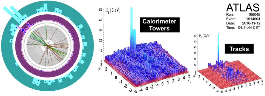
More recently, fully reconstructed jets, which carry the full information of the partonic energy loss, have been measured at the LHC. Dijet events were observed to become increasingly asymmetric in more central collisions, while retaining an angular correlation consistent with back-to-back jets. This result [1] has generated a great deal of excitement, as it strongly suggests the interpretation that back-to-back jets traverse different path lengths in the medium resulting in events with large dijet asymmetry where one jet leaves the medium mostly unscathed while the other experiences significant quenching. An event display of a highly asymmetric event is shown in Fig. 1.1. This observation is the first direct evidence for jet quenching and is one of two results presented in this thesis.
The asymmetry is sensitive to the energy loss of one parton relative to one another, and additional insight into the effects of quenching can be provided by observables that are sensitive to the quenching on a per jet basis. Energy loss of single partons could result in jets emerging from the medium with significantly less energy, resulting in a different final spectrum for events in which the medium is produced. Due to the steeply falling nature of the unquenched spectrum, a systematic downward shift in jet energies due to quenching causes a reduction in the total number of jets at a given . The second result presented in this thesis is a measurement inclusive production of single jets. Ratios of jet spectra in different centrality intervals relative to a peripheral reference were used to construct an observable, , quantifying the extent to which jet production is suppressed by the presence of the QGP through quenching. The has been measured as a function of jet and size as well as collision centrality, which should provide the ability to distinguish between different models of the quenching mechanism.
This thesis is organized as follows. Chapter 2 provides background on both experimental and theoretical developments leading to the conclusion that QCD is the correct theory to describe the strong nuclear force. These ideas are developed to motivate the use of heavy ion collisions as an experimental tool, and various formulations of the jet quenching problem are presented. Chapter 3 describes the experimental apparatuses, the LHC and the ATLAS detector, used to provide the measurements presented in this thesis. Chapter 4 discusses the experimental techniques used to separate underlying event contributions from the jet signal and perform jet energy scale calibrations. Analysis of reconstructed jets is discussed in Chapter 5, including unfolding of the jet spectrum to account for detector effects and estimates of systematic uncertainties. The final results of this analysis, the jet and dijet asymmetry, are presented in Chapter 6 with conclusions following in Chapter 7.
Chapter 2 Background
Nuclear physics deals with the study of the fundamental properties of nuclear matter and the character of the strong nuclear force. By the 1960’s the concept of nuclear matter had been extended from the nucleons making up atomic nuclei to a vast number of strongly interacting particles known as hadrons. The flavor symmetries among various types of hadrons suggested that these particles are composite particles with their quantum numbers carried by common, sub-hadronic objects, and that these objects possessed a new quantum number known as color [2]. A group theoretic approach to hadron taxonomy led to the development of the Quark Model [3, 4, 5, 6, 7] which predicted the baryon observed at BNL in 1964 [8].
Developments in current algebra led to a proposed scaling behavior of the structure functions in deep inelastic scattering. Bjorken Scaling [9] implies that at high momentum transfer, , the hadronic structure functions are independent of and functions of a single scaling variable, . Scaling behavior consistent with this relation was observed in a series of measurements in deep inelastic scattering (DIS) at SLAC [10, 11], leading to the interpretation of point-like constituents within the nucleon known as the Parton Model [12, 13, 14].
Advances in renormalization group techniques [15, 16, 17, 18] led to the conclusion that only a theory possessing asymptotic freedom, a coupling strength that becomes arbitrarily weak at high energies, could be consistent Bjorken Scaling [19, 20]. The symmetry considerations of the Quark Model suggested that non-Abelian gauge theories [21] would be potential candidates for such a theory. These theories were found to possess the required renormalization criteria with the -function in the calculation of the running of the coupling being negative for an SU(3) gauge symmetry [22, 23]. Furthermore, explicit calculations of the anomalous dimensions of the DIS structure functions showed that these non-Abelian gauge theories possessed scaling properties consistent with experimental observations [24, 25, 26, 27].
This description of the strong interaction as an SU(3) (color) gauge symmetry between spin- quarks and mediated by massless spin-1 gluons is known as Quantum Chromodynamics (QCD). At short distance scales, asymptotic freedom ensures that the coupling becomes weak and perturbative techniques can be used to calculate observables. The validity of QCD as the correct theory of the strong interaction has been rigorously demonstrated by a variety of experimental results that are well described by perturbative calculations. A summary of this evidence is presented in Section 2.1.
Color charges are never observed as isolated particles but rather as constituents of color neutral hadrons, an aspect of QCD known as confinement. Furthermore, the QCD Lagrangian possess chiral symmetry which is dynamically broken through the interactions that bind the quarks into hadrons and is responsible for the vast majority of the mass of ordinary matter111This symmetry is only approximate as it is broken explicitly by the quark masses. Thus the pions are pseudo-Goldstone bosons.. However, at soft momentum scales the coupling becomes increasingly large and at hadronic energies the theory is non-perturbative. This leads to significant challenges in theoretical calculations and interpreting experimental results, and much of the work done since the inception of QCD has been to navigate these challenges to develop a comprehensive picture of the strong interaction.
2.1 Experimental Evidence for QCD
Initial experimental evidence for QCD as a theory of the strong interaction was provided in DIS through the observation of Bjorken Scaling. Measurements of the proton structure function are shown in Fig. 2.1, and DIS structure functions in the context of the Parton Model and collinear factorization are further discussed in Section 2.3. Subsequent tests of the theory have been performed in collisions and hadronic collisions, particularly through the Drell-Yan process, the inclusive production of lepton pairs in hadronic scatterings, [28]. These results have provided overwhelming experimental support for QCD [29, 30], and a brief survey is discussed below.

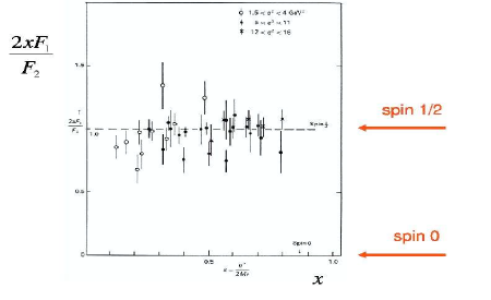
The Callan-Gross [31] relation between the DIS structure functions, , arises due to scattering off spin-, point-like objects; the measured behavior of the structure function, shown in Fig. 2.2, is approximately consistent with this relation.
In collisions the ratio of cross sections for the production of inclusive hadrons to muon pairs is given to leading order in QCD by
| (2.1) |
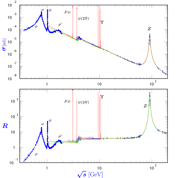
where is the center of mass energy, is the number of colors ( for QCD), and is the charge of quark . The sum runs over the quark flavors up to the heaviest quark capable of being produced at that . This ratio, aside from resonance peaks and away from the threshold, is measured to be approximately constant with discrete jumps at the quark mass thresholds as shown in Fig. 2.3.
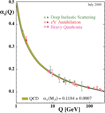
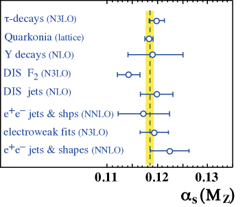
Highly collimated, energetic sprays of particles balanced in momentum known as jets were observed in collisions at SLAC [34], consistent with the hypothesis that hadrons are produced in these collisions through the production of pairs of opposite momentum. The observation of three jet events at PETRA through the process provided experimental evidence for the gluon as well as measurements of the strong coupling constant [35]. Further precision measurements of the strong coupling constant have shown remarkable consistency [36] and a summary is shown in Fig. 2.4.
2.2 Fundamentals of QCD
QCD is the quantum field theory that describes the strong nuclear force, and is expressed in terms of quarks and gluons which contain color charge described by an SU(3) gauge symmetry. The spin- quarks fields, , transform under the fundamental, three-dimensional, representation of the gauge group,
| (2.2) |
with the subscript describing the quark color. The are the generators of the gauge group, represented by eight 33 matrices (, ), and obey the Lie Algebra 222In this section the generator/adjoint indices are denoted by capital, Roman script, as a superscript with the summation over repeated indices is implied. The fundamental, matrix multiplication indices are denoted by lower case, Roman script appearing as subscripts. The Lorentz indices are indicated by Greek characters and the standard Einstein summation convention applies.
| (2.3) |
with the structure constants of SU(3). The local gauge symmetry is imposed by replacing the derivatives appearing in the usual Dirac Lagrangian with the gauge-covariant derivative, ,
| (2.4) |
The color indices and on are explicit here to indicate that the covariant derivative is Lie Algebra-valued (i.e. matrix-valued). The covariant derivative introduces a non-Abelian coupling, of strength , between the quarks and massless, spin-1 gauge fields representing gluons. These transform under the adjoint, eight-dimensional, representation of the gauge group. Including the pure Yang-Mills action for the gauge fields, the full QCD Lagrangian is given by
| (2.5) |
with the index denoting the quark flavor with mass . The field strength tensor is expressed in terms of the gauge field via
| (2.6) |
The QCD vertices are shown in Fig. 2.5. In addition to the analog of the QED gauge coupling shown on the left, the non-Abelian structure of the theory allows for coupling between the gauge fields themselves.

Color factors, associated with different processes, arise from the group structure in the Feynman rules,
| (2.7) |
In QCD, these have values
| (2.8) |
and are typically associated with the splittings , and respectively.
The quantization of this theory is typically performed using the path integral formalism. In this technique, the gauge-fixing condition imposes a constraint on the functional integral which can be removed by the introduction of Faddeev-Popov ghost fields [37]. These unphysical fields appear as an artificial mechanism for preserving gauge invariance. Their contributions, and the contribution of the gluon propagator, will depend on the choice of gauge, with this dependence dropping out in the computation of any gauge invariant quantity.
2.2.1 Ultraviolet Behavior
The ultraviolet (UV) behavior of QCD was the main reason it was originally proposed as the theory of the strong interaction. The relationship among the UV divergences is encoded in the Callan-Symanzik equation. In particular, the derivative of the coupling constant with respect to the renormalization scale, , is defined by the -function,
| (2.9) |
The one-loop -function for SU() non-Abelian gauge theories was first computed by Wilczek, Gross and Politzer in 1973 [22, 23]. For it is given by
| (2.10) |
with . The one and two-loop coefficients are
| (2.11) |
To one-loop, the solution is
| (2.12) | |||
where is used to set the scale of the strong coupling. To higher order in this is
| (2.13) |
where the definition of becomes dependent on the renormalization scheme. The result above is for the scheme [29]. As the renormalization scale is increased the coupling decreases, as indicated by the leading sign in the -function. This property is asymptotic freedom. For general SU(), . The leading, positive term is due to the gluons, which reduce the coupling at large . There is competition, which weakens the asymptotic freedom, from the second term which is due to fermion loops and is proportional to the number of flavors.
2.2.2 Infrared Behavior
Although QCD is well behaved at large momenta, the infrared behavior must be handled with care in perturbative calculations. Since gluons (and to a good approximation the light quarks) are massless, any sensitivity to the long range behavior of QCD appears in perturbation theory as an infrared divergence. Fortunately, the configurations that introduce this sensitivity have been systematically analyzed and a formal procedure exists to define quantities which are infrared safe [38, 39, 40]. These divergences are associated with the contributions to the momentum integration where the massless particle has zero momentum (soft) or at zero angle (collinear). Observables that are safe from these divergences must be insensitive with respect to the emission of an additional soft or collinear gluon. Formally, this means that for an inclusive quantity , defined by the functions ,
| (2.14) |
the quantity is said to be infrared and collinear (IRC) safe if
| (2.15) |
This idea is expanded in the discussion of applications of perturbative QCD in the following section.
2.2.3 Non-Perturbative Dynamics
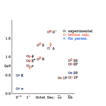
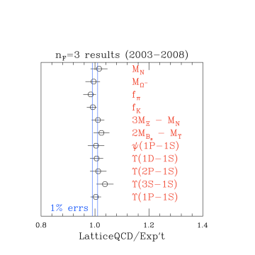
Inspired by Wilson’s picture of renormalization, a discrete lattice formulation of QCD was developed to supplement perturbation theory where the latter is inapplicable [41]. This procedure uses the path integral formalism in Euclidean space-time, where the field configurations are explicitly integrated over. The integration is accomplished by recasting the quantity of interest in terms of gauge links between adjacent lattice sites. The finite lattice spacing, , serves as an ultraviolet cutoff, and a valid lattice formulation must respect all of the features of QCD in the limit . Technical challenges arise as spurious fermion states can be produced in this limit as lattice artifacts [42, 43]. This can be mitigated, although not completely removed, while maintaining chiral symmetry, by introducing staggered fermions [44]. Furthermore, the finite spacing introduces integration errors in the evaluation of the action. These can be minimized by using improved definitions of the action [45]. Advances in computing power and improved actions have led to highly accurate calculations, such as decay constants, form factors and the spectrum of hadrons, which is shown in Fig. 2.6. Additionally, the Euclidean path integral formulation is amenable to calculating thermodynamic quantities in QCD, a topic discussed in Section 2.4.2.
A qualitative picture of confinement is to view the static potential as Coulombic at short distances, but growing at long range,
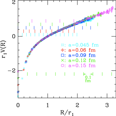
| (2.16) |
A recent lattice calculation of the static quark potential is shown in Fig. 2.7, which indicates behavior approximately consistent with this analytic form.
As the separation between the pair increases the force remains constant, and an increasing amount of energy is stored in the stretched gluon field called a flux tube. At some separation it becomes energetically favorable to break the flux tube and produce a new pair from the vacuum. This process, known as string fragmentation, is shown schematically in Fig. 2.8. Such a mechanism provides a heuristic construct for modeling confinement; no matter how much energy is applied only color-neutral objects can be created from the system. The flux tube picture has led to developments in hadron phenomenology by considering hadrons as relativistic strings [47, 48], and the constant, , in Eq. 2.16 can be interpreted as a string tension. Monte Carlo (MC) event generators for simulating the production of hadrons have had a long history of success using string models [49, 50].

2.3 Applications of Perturbative QCD
2.3.1 The Parton Model and Factorization
QCD has had great success in providing reliable perturbative calculations of experimental observables. The most basic application of QCD uses the parton model, which is a tree-level, impulse approximation to the full perturbation theory. The scattering process is formulated in terms of point-like constituents integrated over probability distributions for a given parton to have momentum fraction ,
| (2.17) |
Here and denote the colliding hadrons and and denoting partons of a particular type. The functions give the probability density of finding a parton of type in hadron with momentum . While asymptotic freedom ensures that at sufficiently hard scales the partonic level matrix elements are calculable in perturbation theory, almost any real world observable will involve hadronic initial and/or final-states, where the theory becomes non-perturbative. The applicability of Eq. 2.17 in certain kinematic regimes suggests that calculations can be performed by separating the short distance behavior of QCD, encoded in the partonic matrix element , from the long range behavior represented by the probability distributions. The formal apparatus through which this is accomplished is known as factorization. Factorization theorems take a similar form to Eq. 2.17 where each term in the integrand is also dependent on a scheme-dependent factorization scale, . This parameter sets the cutoff for which aspects of the dynamics are being included in the description of the long and short range components. The form of the factorization ensures that there is no quantum mechanical interference between the long and short range behavior. Furthermore, the probability distributions, which are known as parton distribution functions (PDFs) in the general factorized formulation, are independent of the specific scattering process. Although they are not calculable by perturbation theory, once these functions are determined experimentally they can be applied to a calculation regardless of the details of the partonic level scattering, thus making them universal features of the hadrons. Factorization theorems have been proven for a variety of processes, among particles and , with the schematic form of the theorem being
| (2.18) |
Here and denote the parton distribution and fragmentation functions (see Section 2.3.4) and represents a convolution over parton momentum fraction, trace over color indices and sum over parton species. This form is traditionally referred to as a twist expansion, with the first term known as the leading twist. The remainder terms, the power suppressed corrections, are suppressed by powers of a hard scale and are referred to as higher-twist effects. Most factorization theorems have been proven using a collinear factorization scheme, where the transverse momentum of the parton has been integrated over. These theorems have been proven in the cases of DIS and , but the only case involving hadron-hadron scattering to have been rigorously proven is the Drell-Yan process [51, 52, 53].
Observables such as spin asymmetries in hadronic collisions provide access to the spin structure of the proton. However, the extension of the usual collinear formalism in these cases has been problematic [54, 55, 56, 57] as the observables contain sensitivity to the transverse momentum dependence (TMD) of the PDFs. Without integrating over the transverse dependence of the PDFs, gauge links couple soft and collinear portions of diagrams to the hard sub-graphs, breaking the factorization. Attempts to construct TMD factorization schemes, such as -factorization [58, 59], have proven difficult and it has been shown explicitly that -factorization is violated in high- hadron production in hadronic collisions [60]. Building a framework to perform these types of calculations is still a subject under active development [61].
2.3.2 Deep Inelastic Scattering
The parton model was first developed in DIS, and this collision system will be used here to illustrate the utility of the factorized approach. In these collisions an electron interacts with a hadronic target of mass via the exchange of a photon with large virtuality . In addition to , the system is typically described in terms of the variables and
| (2.19) |
where is the four-momentum of the target and and are the initial and final energies of the electron as measured in the rest frame of the target. In the parton model, corresponds to the fraction of target’s momentum carried by the struck quark. The differential cross section is usually expressed in terms of structure functions ,
| (2.20) |
The observation of Bjorken scaling [10, 11], that for large , and are independent of , was the inspiration for the parton model. For spin- (charged) partons, the structure functions obey the Callan-Gross relation . The experimental confirmation of this result provided support for the interpretation of spin- quarks. In collinear factorized form the structure functions have the form,
| (2.21a) | |||
| (2.21b) |
Here the functions are the PDFs for parton in hadron . The coefficient functions, , are calculable in perturbation theory and are IRC safe. They are dominated by contributions of order ; propagators off shell by will contribute to while contributions below this scale are grouped into . The result depends on both the factorization and renormalization scales, which need not be set equal.
Shortly after the computation of the -function, similar renormalization group techniques were applied to the DIS structure functions, by considering moments of the PDFs (specifically non-singlet PDF, ),
| (2.22) |
These are related to the anomalous dimensions,
| (2.23) |
which appear to give dimensions to dimensionless, but scale-dependent quantities through renormalization (e.g. ), and can be computed in perturbation theory [20]. The -dependence of the PDF moments can be used to determine the -dependence of the moments of the structure functions,
| (2.24) |
This relation predicts power-law scaling, , for theories that do not possess asymptotic freedom and posed a problem reconciling potential theories with the observed scaling prior to the demonstration of asymptotic freedom in QCD. To one-loop in QCD the scaling is [24, 25, 26, 27]
| (2.25) |
This weak -dependence correctly described the early measurements of scaling in DIS, further building support for QCD as the correct theory of the strong interaction.
2.3.3 DGLAP and Parton Evolution
When calculating , logarithms can arise due to the collinear emission at some scale , which gives a factor of approximately
| (2.26) |
These logarithms can become large such that the above product becomes of order unity. The result is that will have large contributions from all orders and is shown schematically in Fig 2.9. This multiple emission is enhanced by , but only for the case where the virtualities are strongly ordered, , with other orderings appearing with fewer powers of .
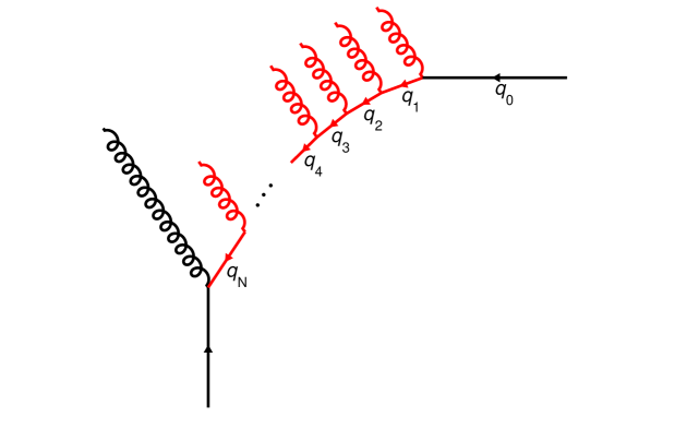
The large logarithms are a symptom of interactions far away from the scale at which the coupling was fixed. Fortunately, these collinear contributions can be resummed by renormalization group methods. As most of the collinear emissions are well separated in scale from the probe, , these emissions can be reinterpreted as modifying the hadron structure as opposed to corrections to . This results in a -dependence of the PDF that evolves the probe from the hard scale to lower momentum scales (indicated by the red sub-diagram in Fig 2.9). For the change the differential probability of an emission with energy fraction and transverse momentum is given by
| (2.27) |
where is the splitting function for parton of splitting into type , and can be computed from the diagrams shown in Fig 2.10. Changes in the distribution of parton at momentum fraction can come from splittings of other partons at , and can be written as

These lead to the DGLAP evolution equations [62, 63, 64] which are of the form
| (2.29) |
See Ref. [30] for a complete tabulation of the splitting functions and full evolution equations. This result indicates that if is measured as a function of at a given value of , the PDF at any other scale can be determined by evolving the PDF according to Eq. 2.29. The dependence of the structure function at fixed is shown in Fig. 2.1. This dependence agrees well with the dependence predicted by the DGLAP equations over a range of and values.
2.3.4 Fragmentation Functions
The final-state analog of the parton distribution function is known as a fragmentation function. The fragmentation function encapsulates the probability that a parton of type will fragment into a hadron of type with momentum fraction of the original parton. In collisions, where there are no initial parton distributions, cross sections for the production of a particular species of hadron can be written as,
| (2.30) |
For situations with arbitrary numbers initial/final-state hadrons, the collinear factorized relation takes the form of Eq. 2.18. The measurements provide the cleanest access to the fragmentation functions since there is no integration over PDFs. The fragmentation functions obey an evolution equation in identical to Eq. 2.29, with the inverse splitting functions (i.e. is replaced with ). In the parton model these obey the momentum sum rule,
| (2.31) |
The higher-order corrections to the splitting functions can see logarithmic enhancements at low , an effect which causes the leading order approximation of the evolution to break down much sooner in than DIS. This has led to development of calculations using a modified leading log approximation (MLLA), which include corrections for next-to-leading effects [65, 66, 67, 68, 69]. In general, the behavior of these enhancements is to cause the “hump-backed plateau” behavior,
| (2.32) |
with and the width and peak approximately given by [70],
| (2.33) |
This behavior is shown in Fig. 2.11, with the fragmentation functions fit with a Gaussian for a variety of and values shown on the right and a comparison of the extracted peak position to the MLLA value shown on the left.


To span a large kinematic range and provide separation between quark and anti-quark contributions, the data has been supplemented by DIS and hadronic collider data in recent global NLO extractions [71, 72, 73] (see 2.3.5 for discussion of fixed order calculations). A comparison of results of some such analyses are shown in Fig 2.12, where the various partonic contributions to the charged pion fragmentation function are shown.

2.3.5 Fixed Order Calculations
Perturbative calculations are typically performed at fixed order and it is useful to consider IRC safety in this context [30]. For an -particle process, the cross section for an observable, , can be constructed at leading order (LO) as
| (2.34) |
where is the -particle matrix element at tree-level, is the measure over the -particle phase space and is the renormalization scale. Non-perturbative corrections have been omitted here. The tree-level amplitudes are finite but the integral will diverge in the soft and collinear regions of the momentum integration. Therefore this calculation is only safe when also vanishes in this limit (e.g. jet cross sections). At next-to-leading-order (NLO) the -particle matrix element must be considered along with the interference between the tree-level and 1-loop -particle processes,
Here is the 1-loop -particle amplitude, which diverges in the soft and collinear limits. This divergence will cancel with the aforementioned tree-level divergence in the integration if the observable is IRC safe,
| (2.36) | |||
A similar procedure applies in extending to NNLO calculations, which involve additional contributions the tree-level contribution, interference between tree-level and 1-loop -particle diagrams, interference between the -particle tree-level and 2-loop diagrams and the squared contribution of the 1-loop -particle diagram. These calculations become increasingly difficult to compute, especially in an automated fashion, due to the intricate higher-loop diagrams.
Often these calculations are supplied in the form of Monte Carlo event generators. These tools typically compute a hard scattering matrix element and then evolve the partons by means of a parton shower. This technique constructs a probability for a parton not split from the splitting functions defined in Eq. 2.27. The probability that a parton of type will not split between scales and , , known as a Sudakov form factor is given by,
| (2.37) |
MC sampling determines the scale of the first splitting, and this process is repeated down to some hadronization scale GeV. At this point a hadronization model [49, 50, 74, 75] converts the evolved partons into final-state hadrons which can be used to simulate response of a detector to an input physics signal. Leading order event generators (e.g. PYTHIA) typically give the correct description of the soft and collinear emission, but fail to describe wide angle emissions due to the lack of multi-parton matrix elements. This can be improved by generators which use this higher order matrix elements and merge the parton showers in such a way as to avoid double counting the real and virtual contributions [76, 77, 78, 79].
In general LO calculations for applications at hadron colliders are accurate to approximately a factor of two. A -factor, which represents the ratio of NLO to LO contributions, is typically used to tune the cross sections.
2.3.6 Jets
Highly collimated sprays of particles known as jets are a ubiquitous feature of high energy particle collisions. These objects are the experimental signature of partonic hard scattering processes and have been used to test the theoretical application of the theory since their initial observation at SLAC [34]. However, the multi-particle final states associated with jet production are sufficiently complicated that any experimental measurement must have a precise definition of an observable [38]. Furthermore, these definitions must be relatable to quantities that are well-defined theoretically, particularly with regard to the IRC safety issues discussed previously.
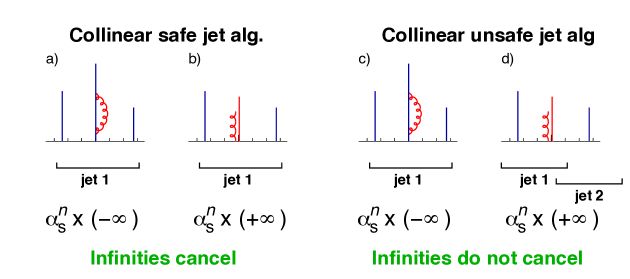
Most early jet algorithms were based on associating particles or energy deposits that were nearby in angle, typically referred to as cone algorithms. The Snowmass workshop in 1990 [80] proposed a standard set of criteria for jet algorithms [81], however implementations of these criteria were not immediately obvious. Many cone algorithms used at the time suffered from varying degrees of IRC unsafety, which limited their relatability to theory [82]. The effects of unsafety are illustrated in Fig 2.13, where two algorithms, one safe (left) and one unsafe (right) are compared. In the IRC safe algorithm, the emission of a collinear gluon does not affect the clustering (b), allowing the divergence in this graph to cancel the 1-loop (a) divergence. However, this emission causes different clustering in the unsafe algorithm (d), resulting in a failure in cancellation of the divergences. In general, issues of split or overlapping jets are not handled in a natural way by cone algorithms, and some additional criteria, often introducing undesired artifacts, are required to handle such cases.
Sequential clustering algorithms, which perform pairwise clustering of particles [84, 85], showed particular promise as they were IRC safe. This led to the proposal for the algorithm in collisions [86], which was formulated to be boost-invariant and IRC safe and was later adapted for hadronic collisions [87]. The inclusive formulation of this algorithm [88] uses the measure,
| (2.38) |
where and are the particles’ rapidity and azimuthal angle respectively, to cluster nearby particles. The algorithm works using the following steps:
-
1.
Calculate for all pairs and also .
-
2.
Find the minimum of the and .
-
3.
If the minimum is a , combine and and start over.
-
4.
If the minimum is a , call a final-state jet and remove it from subsequent clustering and start over.
-
5.
Finish clustering when no particles remain.
The parameter controls the size of the jets in analogy with the radius parameter in cone jets. In this inclusive form, all particles are clustered into final-state jets; thus some final discriminating criteria, often a minimum cut on or , must be applied. This algorithm has the feature that for soft or collinear pairs the distance measure is inversely proportional to the differential probability of collinear emission,
| (2.39) |
which is easily adaptable to theoretical
calculations [82]. This algorithm was not originally
favored by experiment due to its slow processing time and
geometrically irregular jets, which made experimental corrections more
difficult. However, a faster implementation by the FastJet package(
vs. ) has significantly improved the former
issue [89].
The distance measure of the algorithm can be generalized in the following way:
| (2.40) |
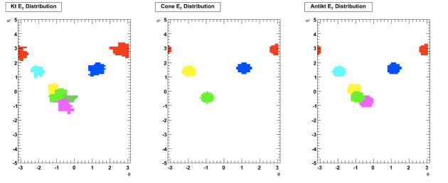
The choice corresponds to the usual algorithm, while corresponds to the Cambridge/Aachen algorithm [90, 91], which uses only geometric considerations when clustering objects. The generalization was used to define the anti- algorithm (), which clusters hard particles first and produces jets similar with regular, cone-like geometry [83]. Examples of the clustering behavior of the , ATLAS cone [92] and anti- algorithms are shown Fig. 2.14. The allows jets clustered from soft background particles to compete with the real jet signal, a feature which is particularly problematic in heavy ion collisions. This is contrasted by the behavior of the anti- which preferentially clusters particles with the harder of two jets.
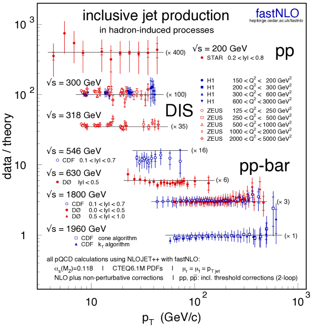
Jets have become an essential part of high energy experiments, both as
tools for testing QCD, but also as input into reconstructing more
complicated physics objects. Figure 2.15
shows the data/theory ratio for the inclusive jet cross
section as a function of jet for a wide range of experiments. The
theoretical calculation is provided by fastNLO with NLOJET++ [93].
2.4 Phase Structure of Nuclear Matter
Prior to the advent of QCD, attempts were made to apply statistical methods to the large particle multiplicities in high energy collisions [94, 95]. This led to the analysis of the high temperature limit of nuclear matter in the context of hadronic resonances. The growth in the number of these resonance states with increasing energy led Hagedorn to propose the Statistical Bootstrap Model, where resonances are thought of as being composed of excited lower mass resonance constituents. In the high temperature limit the density of resonant states and the thermodynamic energy density of states approach each other and the partition function diverges. The temperature cannot be increased beyond some limiting value, the Hagedorn temperature, as adding energy will only excite more resonances, not add to the kinetic energy of the system [96].
Asymptotic freedom indicates that this will not occur, but rather that at sufficiently high temperatures the coupling will become weak leading to nuclear matter with dynamics described by perturbative QCD [97]. This suggests that there is a phase transition where the degrees of freedom evolve from hadrons to quarks and gluons. This state of matter the Quark Gluon Plasma (QGP), represents the form of nuclear matter in the early stages of the Universe [98].
In the weak coupling limit the Stefan-Boltzmann relation between energy density, , and pressure, , applies:
| (2.41) |
Each is proportional to with the constant of proportionality indicating the degeneracy of particles obeying Bose-Einstein, , and Fermi-Dirac, , statistics,
| (2.42) |
At the lowest temperatures the system is hadron gas containing only the lowest state, the pions (, ). At high temperature the system is a gas of deconfined quarks and gluons (, ). The total energy density is
| (2.43) |
For two flavor QCD the difference in phases corresponds to a factor of 9 increase in , indicating a dramatic change in energy density.
The temperature range over which this transition occurs, specifically the possible divergences of thermodynamic variables, can characterize the transition. In the limit of zero quark mass, the QCD Lagrangian possesses chiral symmetry, which is broken by non-perturbative effects resulting in three massless pions. The high temperature limit exhibits both deconfinement and restoration of chiral symmetry, and it is unclear to what extent these two phenomena are interrelated and whether QCD may exhibit a distinct phase transition associated with each of these phenomena [99].
2.4.1 Thermal Field Theory
The extension to finite-temperature field theory is accomplished by using the relationship between the path integral formulation in quantum field theory and the partition function of statistical mechanics [100, 101]. Explicitly, the path integral for a single quantum mechanical particle with Hamiltonian is given by
| (2.44) |
which denotes the amplitude for a particle at at to go to at , and . This functional integral can be analytically continued to imaginary time via . This generally provides a more rigorous definition for the path integral and its convergence. In the imaginary time formulation the action in the exponent is replaced by the Euclidean action
| (2.45) |
where . This can be compared directly to the partition function of the canonical ensemble, with temperature and , . In the non-diagonal basis this can be written in the same form as the usual path integral,
| (2.46) |
Thermal expectation values of time-ordered products of fields can be computed in the same fashion as zero-temperature field theory, but using the imaginary time/Euclidean action. For example, a generating functional, , can be constructed by introducing a source , and adding the term to the Lagrangian. A two-point correlation function can be evaluated with functional derivatives with respect to ,
| (2.47) |
The cyclic nature of the trace imposes the constraint , with the sign depending on whether the field obeys commutation or anti-commutation relations. Thus the periodic (anti-periodic) boundary conditions on the correlation functions enforce the Bose-Einstein (Fermi-Dirac) statistics and can be described as a Fourier series
| (2.48) |
Here for bosons and for fermions and are known as the Matsubara frequencies. The full real-time gauge theory propagators at tree level are
| (2.49a) | |||
| (2.49b) |
for the bosons and fermions respectively. In both expressions, the first term describes the usual vacuum propagation while the second represents the disconnected part of the propagation which counts the modes absorbed by the medium.
2.4.2 Lattice Thermodynamics
The lattice formulation of QCD discussed previously can be naturally applied to calculate thermodynamic variables in QCD, since it is formulated as a Euclidean space-time evaluated path integral. The four-dimensional Euclidean space-time is represented by lattice sites with spacing . The system is described by volume and temperature, ,
| (2.50) |
and the thermodynamic limit is taken with , but holding fixed. Statistical errors can enter since the integration is performed over a finite number of gauge field configurations, thus making calculations with large difficult. Recent developments in improved actions with reduced discretization errors allow for accurate calculations without resorting to large , and have facilitated advances in lattice thermodynamic calculations.
Typically the action is separated into a contribution from the gauge fields and a fermionic contribution. The latter is expressed as a functional determinant in a way that removes or minimizes fermion doubling problems. The action and determinant are written in terms of link variables, which involve the evaluation of gauge field configurations at adjacent lattice sites. The numerical integration techniques require a probabilistic interpretation, and problems occur when the determinant becomes negative. For zero chemical potential, , this is not a problem, however the determinant becomes complex-valued for . This makes calculations at finite chemical potential more difficult, although recent advances have been made on this subject.
The QCD equation of state can be determined on the lattice by evaluating the trace anomaly (the trace of the stress-energy tensor ) in the grand canonical ensemble,
| (2.51) |
Since only expectation values can be calculated, the variables must be re-expressed in this form. The pressure can be evaluated directly from integrating the trace anomaly. The entropy density, , and speed of sound , can likewise be calculated from the relations
| (2.52) |
The pressure and energy density divided by from a recent calculation [102] are shown in Fig. 2.16.
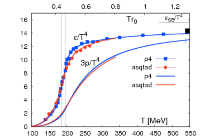
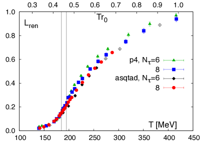
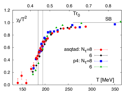
The lattice results indicate a rapid, but continuous transition in at MeV, which is not indicative of a first or second order phase transition, but rather a smooth crossover between phases. Additionally, order parameters describing the transition to deconfinement and the restoration of chiral symmetry have been formulated on the lattice. The deconfinement order parameter is the expectation value of the Polyakov loop, where is the static free quark energy. The chiral transition is described by the chiral susceptibility . These quantities involve subtleties relating to their renormalization and corrections due to finite quark masses. A calculation of these two quantities [102] is shown in Fig. 2.17. The results indicate that both of these transitions occur smoothly over the same temperature region where the equation of state shows a rapid change in energy density.
2.4.3 The Hard Thermal Loop Approximation
When using perturbation theory at finite temperature, including the effects of loops becomes problematic as the finite scale introduced by breaks the usual perturbative expansion. If the external momenta are hard, all loops will contribute to the same order as the tree level diagram. However if the external momenta are soft, , only the contribution from Hard Thermal Loops (HTLs) will compete with the tree level term. These are cases where the “hard” loop momenta are much greater than the “soft” external momenta and the dominant contribution to the loop comes from momenta of order . In gauge theories, the HTLs can be identified by power counting and an effective theory of resummed HTLs can be derived without affecting the vacuum renormalizability properties of the theory [103, 104]. These loops lead to the generation of thermal masses and for the gauge bosons and fermions respectively. The static component of the gauge boson propagator takes the form
| (2.53) |
where the thermal mass gives rise to Debye screening. In the static limit, , the magnetic behavior is similar to the above expression, but with
| (2.54) |
This can be interpreted as a frequency-dependent dynamical screening with cutoff , which is in some cases effective in protecting infrared divergences [105]. The full thermal masses including the effects from a finite chemical potential, , are given by
| (2.55a) | |||
| (2.55b) |
with the color factors given previously in Eq. 2.8.
One issue that is still not fully understood is the screening of the chromomagnetic fields. Using power counting arguments it can be shown that a diagram containing gluon loops, shown in Fig. 2.18, with , has infrared divergences of the form [106]
| (2.56) |
For the longitudinal components this is regulated by the electric mass and gives behavior , which differs from the behavior expected from perturbation theory. Based on arguments from theories that are infrared-equivalent to QCD, the magnetic mass is of order [107]. This leads to infrared divergences in the transverse part of the gluon loop diagram to go as and signals a total breakdown of perturbation theory. This remains an outstanding problem, with thermal field theory not on rigorous theoretical ground except at asymptotically high temperatures.

2.4.4 Heavy Ion Collisions
The phase structure predicted by the lattice indicates that at low baryon chemical potential and high temperature, hadronic matter undergoes a rapid, but continuous increase in the number of degrees of freedom. This transition is illustrated in a possible QCD phase diagram, shown in Fig. 2.19.
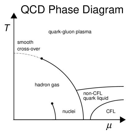
In addition to this transition, abnormal forms of nuclear matter can exist at high densities [108, 109]. Astrophysical objects such as neutron stars are stabilized against gravitational collapse by the degeneracy pressure created by an extremely high density of neutrons. At the highest densities novel states such as quark liquids and color superconductors (color flavor locked) are thought to exist [110].
It is believed that the QGP transition is experimentally accessible in collisions among heavy ions at high energies. In these collisions the nuclei appear as highly Lorentz contracted “pancakes” [111]. Particle production occurs as the two pancakes overlap leaving a “central” region of high energy density as they recede and carry away the net baryon density (leading baryon effect). If the system is formed after some time , the energy density in this region can be estimated following the Bjorken procedure by considering the total energy per unit rapidity in nucleus-nucleus collisions, . The energy density is then
| (2.57) |
For a small slice along the beam direction , and . is the nuclear radius and behaves as fm. The energy density can be expressed as
| (2.58) |
For collisions at RHIC, was measured by PHENIX to be 688 GeV at GeV [112]. If the formation time is on the order of fm, this procedure gives an energy density estimate of . The Stefan-Boltzmann equation of state can be used to infer a temperature,
| (2.59) |
where is a constant of proportionality determined by the effective number of degrees of freedom. Since the lattice results indicate that this limit is not reached a more appropriate estimate would be to use the lattice value of , just above the transition region. This estimate gives a temperature of MeV. The transverse energy density in Pb+Pb collisions at the LHC at TeV is larger than at RHIC by roughly a factor of , indicating a temperature range of MeV. As the temperature region of the phase transition is spanned by these estimates, it is likely that such a transition is probed in relativistic heavy ion collisions.
If the mean free path in the interacting system is small compared to the system size a hydrodynamic description can be applied to the created nuclear matter [95]. The evolution of the system in the absence of viscosity or heat conduction is described by ideal hydrodynamics,
| (2.60) |
where is the relativistic stress-energy tensor, is the local four-velocity of a fluid element and the system of equations is closed by a thermodynamic equation of state. The Bjorken picture considers the longitudinal expansion of this medium which leads to a slow decrease in the temperature, , where is the local fluid proper time, and constant entropy inside the co-moving fluid volumes.
Local anisotropies in the transverse density of produced particles can be produced through initial-state fluctuations or more commonly through the elliptical geometry of the collision zone when there is incomplete nuclear overlap. As the particle production is isotropic, the only way this can be converted to a momentum-space anisotropy, is if these density fluctuations form pressure gradients, which result in radial flow. Such an effect should be observable in the angular distribution of hadrons and may allow for a determination of the fluid’s shear viscosity, .
Calculational techniques in string theory have established a correspondence between quantum field theories and their dual gravity theories. This AdS/CFT correspondence facilitates a translation between quantities in a gravity calculation in the weakly coupled region to quantities in the strongly coupled regime of the appropriate dual [113, 114]. In particular the thermodynamics of black hole can be mapped to thermodynamics in QCD-like supersymmetric Yang-Mills theory. Some time ago, arguments based on the uncertainty principle suggested that there is a quantum lower limit to the viscosity [115]. This has been demonstrated explicitly in the AdS/CFT picture where a limiting value of the viscosity to entropy density ratio was found to be [116, 117].
This application of hydrodynamics illustrates how the transport properties of the system can provide further insight into the dynamics of the medium, in particular through transport coefficients such as the shear viscosity, which are sensitive to the microscopic behavior. As a transport phenomenon, hydrodynamics coincides with the long-wavelength behavior of the system and the relevant transport and other phenomena such as radiation and diffusion can provide access to other aspects of the medium.
2.5 Hard Processes in Nuclear Collisions
2.5.1 The Glauber Model
In collider experiments, the measured rates of quantities are proportional to the luminosity, or instantaneous flux of colliding particles. At high energies, the nuclear size is easily resolved, and a beam constituent not only sees a flux of nuclei but an instantaneous flux of nucleons/partons determined by the geometric overlap between the colliding nuclei. For two nuclei, and , with centers separated by impact parameter , this flux is represented by the factor . Many nuclear effects are expected to vary with , and is often used to normalize quantities to remove any variation due to trivial geometric effects. Experimentally, events are grouped into different centrality classes, which are determined to have a similar amount of geometric overlap based on a set of global event criteria. The average is used to normalize quantities observed in those events to assess the centrality dependence of an observable. This procedure makes use of a framework known as the Glauber Model [118, 119, 120] and is employed by nearly all heavy ion experiments [121].
The Glauber Model treats the incoming nuclei as smooth distributions of nucleons, each traveling on independent linear trajectories. It is formulated in the optical limit, in which the overall phase shift is evaluated by summing over all per-nucleon pair phase shifts. It relies on a parametrization of the nuclear density, , typically a two-parameter Woods-Saxon distribution,
| (2.61) |
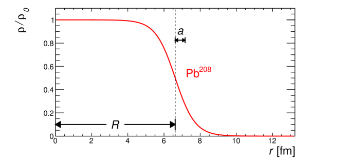
where and are experimentally determined parameters, describing the radius and skin depth of the nucleus. The constant is an overall normalization factor ensuring the distribution is normalized to the number of nucleons. For these parameters are fm, fm [122] and the distribution is shown in Fig 2.20.
In the Glauber formalism the transverse density,
| (2.62) |
is the expected number of nucleons at position . Then is defined as times the probability to simultaneously find nucleons in nuclei and at the same position as shown in Fig. 2.21,
| (2.63) |
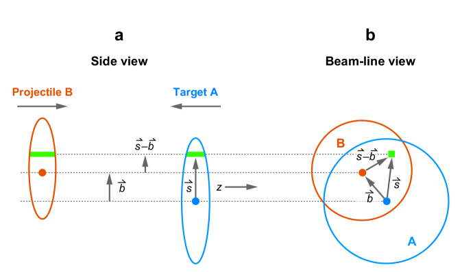
Each nucleon in can interact with a nucleon in with probability , so the total probability of collisions is binomial and is given by
| (2.64) |
This allows for the definition of the expected number of collisions as , and the expected number of participants , the total number of nucleons that participated in any scatterings (sometimes referred to as wounded nucleons) as
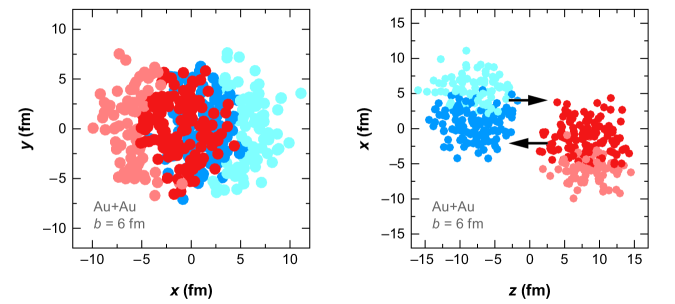
An alternative to performing the analytic integrals is to use Monte Carlo techniques. This has the advantage of including terms neglected in the optical approximation that incorporate local per-event density fluctuations [123, 121]. This method is performed by sampling the full Woods-Saxon distribution in Eq. 2.61 times to populate positions for nucleus . To prevent overlap, a position is regenerated if it is found to be within some minimum distance of a previously generated nucleon. Once the positions have been generated for both nuclei, a random impact parameter vector is generated defining an offset between the nuclear centers. The transverse position for all nucleons in nucleus is compared to each of the analogous nucleons in . If the distance between the pair is , the nucleons are considered to have participated. is defined as the number of times this condition is satisfied, with defining the number of nucleons for which this condition was satisfied at least once. An example of an event generated with this technique is shown for an Au+Au collision in Fig 2.22.
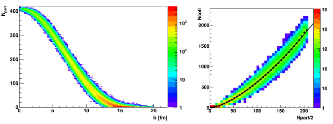
The distribution of values for different impact parameters is shown in Fig. 2.23, as well as the relationship between and .
Experimentally, the per-event impact parameter is not measurable so a procedure must be performed to relate a distribution of some measurable quantity to the Glauber parameters. Variables like the total charged particle multiplicity or transverse energy typically have distributions similar to the and distributions. This feature, combined with the fact that these are global variables and therefore less sensitive to detailed features and fluctuations make them excellent choices for centrality variables. The centrality determination procedure considers the minimum bias distribution of such a variable, , and divides the range of observed values into sub-ranges where the integral of the distribution over that range is some percentage of the total; an example of this division is shown in Fig 2.24. These sub-ranges are called centrality intervals, and centrality-dependent observables are usually calculated by averaging over all events in the same interval.
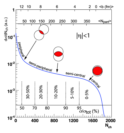
The centrality bin, , is typically defined in terms of percentages, , such that:
| (2.66) |
The Glauber model parameters must then be related to the class of events in a particular centrality bin. This can be accomplished by constructing a new variable, , from the Glauber variables and such that the distribution is similar to the experimentally observed distribution. The distributions tend to be similar enough to the and distributions that a simple linear combination of the two, a two-component model, is a suitable choice for ,
| (2.67) |
The parameters and can be determined from fitting the measured distribution with from an MC Glauber sample. The centrality bins for are defined in terms of integral fractions just as for . In the centrality bin, the and are averaged over all events for which . These and values are then associated with the centrality bin in the data.
2.5.2 Nuclear Modification
The first evidence for modification in nuclear collisions at high energy was observed p+A collisions, where it was found that the production of particles at large transverse momentum ( GeV) was enhanced in these collisions relative to [124, 125]. This effect, Cronin enhancement, was originally interpreted as additional transverse momentum, , imparted by additional, independent, elastic interactions with multiple nucleons. Here is the average path length, which scales with atomic number as .
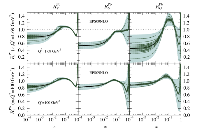
The nuclear parton distribution functions (NPDFs), show both a suppression at lower values of and an enhancement with increasing with respect to the nucleon PDFs, termed shadowing and anti-shadowing respectively. This nuclear modification is quantified through the ratio,
| (2.68) |
where are the PDFs for the nucleus and the nucleon, and is the parton species: valence quark, sea quark or gluon. When viewed in the rest frame of the target nucleus, the shadowing/anti-shadowing is the result of multiple scattering processes that destructively/constructively interfere at the amplitude level [126]. In the collinear factorized approach coherent multiple scattering terms are suppressed by powers of , however for a large nucleus these contributions receive an enhancement of , leading to sensitivity to higher twist effects [127].
When viewed in the infinite momentum frame, the shadowing effects arise from recombination of low- gluons in the nuclear wave function [128]. This phenomenon is known as saturation and sets in as unitarity requirements force the nominal evolution equations to be modified at small . The gluon distribution, , represents the number of gluons per unit rapidity in a region of transverse size and grows as for small at fixed without this modification. However, as , where is the radius of a nucleon, the gluons will begin to overlap and recombination of these gluons will limit the growth of with decreasing [129, 130].
At larger values of , away from the shadowing/anti-shadowing region (), the NPDFs exhibit additional suppression which is known as the EMC effect [131]. The origin of this effect may be related to non-nucleon degrees of freedom in the nucleus [132] and has led to increased interest in short-range correlations between nucleons. A sharp enhancement of the NPDF at the largest values is thought to be described by the Fermi motion of the nucleons. Global analyses at NLO have been performed using data from DIS, Drell-Yan and d+Au collisions at RHIC to extract the -dependence of , and at multiple values [133]. These distributions, shown for Pb in Fig. 2.25, are a crucial input to any interpretation of any high- phenomena observed in nucleus-nucleus collisions.
2.5.3 HIJING
The phenomenology underlying the implementation of event generators such as PYTHIA, requires extensions to be appropriate for nucleus-nucleus collisions. An important step in achieving this was the development of the HIJING MC event generator [134]. To correctly model the multiplicity fluctuations the soft production mechanism combines elements of different models. It introduces multiple, sea strings as in the dual parton model [135, 136, 137], but also allows for induced gluon bremsstrahlung by introducing string kinks as in the Lund FRITIOF procedure [138, 139]. Additional transverse momentum kicks are applied that are dependent on the particle’s proportional to .
The production of “minijets” with GeV is expected to play an important role in the total energy and particle production [140, 141]. These processes take place at an intermediate momentum scale, lower than that associated with typical jet production, but still describable by perturbative QCD. Production of multiple jets in HIJING is implemented through a probabilistic model of independent jet (pair) production. The average number of minijets at impact parameter is given by , where is the inclusive cross section for jets in nucleon-nucleon collisions, integrated above some threshold . The probability for multiple independent minijet production is given by [142],
| (2.69) | |||
| (2.70) |
where is the non-perturbative inclusive cross section for soft processes and is the partonic overlap function between two nucleons separated by impact parameter . An eikonal picture is used to relate the inelastic, elastic and total cross sections and to define the multi-jet probabilities for minijets in nucleon-nucleon collisions,
| (2.71) | |||
| (2.72) |
Here the eikonal factors are related by , and ensure geometric scaling. The independence of the multi-jet production is an appropriate ansatz if . The overall jet cross section is reduced from the nucleon-nucleon case to include the effects of nuclear shadowing, including the impact parameter dependence which has not been measured by experiment. The modification factor defined in Eq. 2.68 can be generalized to include impact parameter dependence,
| (2.73) |
where , models the impact parameter dependence [134]. Then the effective jet cross section is a function of the transverse positions of each of the colliding nucleons in the binary system,
| (2.74) |
The event generation proceeds by using an MC Glauber setup to determine the set of colliding nucleon pairs. For each of these binary collisions, the probability of scattering and number of jets is determined, along with whether the collision is elastic or inelastic. Hard scattering partons are treated separately, and their energies are subtracted from the nucleons with the remaining energy used in processing soft string excitations. The resulting scattered gluons are ordered in rapidity and color-connected to the valence quark/di-quark of the nucleon. The correlated semi-hard particle production mechanism is the key feature of HIJING and is why it has remained a useful tool long after its inception.
2.5.4 Jet Quenching
A significant form of nuclear modification occurs in heavy ion collisions where the byproducts of hard scatterings can interact with the QGP through the phenomenon of jet quenching. The character of this interaction provides key insight into the dynamics of the medium. The most important is the identification of the relevant scales for the jet-medium interaction and whether it can be described by perturbative QCD. If so, it provides a key testing ground for thermal, perturbative QCD and the HTL formulation as well as an example of the transport phenomena of radiation and diffusion in a fundamental physical system.
The potential for jets as a tool to study the plasma was first recognized by Bjorken [143], who suggested that events with back-to-back jets would be sensitive to differential energy loss if the two partons had different in-medium path lengths. In extreme cases a highly energetic jet may emerge while its partner deposits all of its energy in the medium, which would represent a striking experimental signature.
The energy loss mechanism originally proposed by Bjorken was through elastic collisions with the medium constituents. This was originally given in Ref. [143] as,
| (2.75) |
with more intricate forms of the term inside the logarithm due to improvements in the collision integral given in Refs. [144, 145, 146]. In a QCD plasma, the Debye screening mass, , is given by,
| (2.76) |
Some of the first predictions of jet quenching signatures involve a modification of the dijet acoplanarity distribution in heavy ion collisions [147, 148]. These calculations were formulated in terms of the probability distribution for dijet pairs to have momentum imbalance ,
| (2.77) |
The acoplanarity was expected to show a temperature-dependent modification due to elastic collisions with the medium constituents. It was shown that similar effects could be produced through collisional energy loss in a hadronic resonance gas [149], and thus an observed modification would not prove the presence of a QGP phase.
Interactions with the medium can also induce radiative energy loss through the emission of bremsstrahlung gluons. In QED, energy loss for high energy electrons is typically in the Bethe-Heitler regime , where is a characteristic length. Classically, the total energy loss per scattering is the integral of the bremsstrahlung spectrum
| (2.78) |
with multiple scatterings adding incoherently to give a total energy loss
| (2.79) |
where is the medium opacity and is the mean free path between scattering centers.
Most models use a formalism that treats the medium as a series of static scattering centers with the parton and radiated gluons with energies, and respectively, traveling along eikonal trajectories. This is combined with the kinematic limits , where is the momentum transfer with the medium. This kinematic regime is referred to as the soft eikonal limit [150]. The radiation spectrum is typically derived by using the single gluon emission kernel as a Poisson probability for multi-gluon emission.
At high energies, significant interference occurs between the parton and quanta emitted at small angles. This results in a finite formation time for the radiation and suppresses this contribution relative to incoherent radiation, known as the LPM effect [151, 152] in QED. The QCD analog of this phenomenon has been proposed as an important feature of the quenching mechanism [153, 154] and was shown by BDMPS [155] and independently by Zakharov [156] to give an energy loss that grows quadratically with path length in the medium .
As the interference suppresses the coherent radiation, the emission spectrum will be dominated by those quanta which have decohered. These are gluons which have acquired a phase, , of order unity [157, 158],
| (2.80) |
and thus appear with a characteristic energy,
| (2.81) |
Here the transport coefficient has been introduced, which in this picture represents the mean squared transverse momentum imparted to the parton per unit length, .
In this picture the energy loss is determined by soft multiple scattering. In the coherent limit the parton undergoes Brownian motion with a Gaussian elastic cross section , and the scattering centers behave as a single source of radiation. The bremsstrahlung spectrum is given by
| (2.82) |
which results in energy loss . The dependence is qualitatively different than both the Bethe-Heitler energy loss and the LPM effect in QED ().
Other models frame the energy loss as an expansion in opacity. These models are not restricted to small momentum transfers, including the power-law tail in the scattering cross section, but the coherence effects of BDMPS-Z formulation must be enforced order-by-order in opacity. The GLV [159, 160] model is an example of this approach, which models the scattering centers as screened Yukawa potentials with screening length, . The gluon spectrum is constructed by integrating first over the longitudinal direction to enforce the LPM interference at a given order. The momentum transfer is then averaged over giving the double-differential gluon distribution, . This can be analyzed to give information about the transverse pattern of radiation before integrating over and to give the full energy loss.
The ASW formalism [161, 158] is a path integral formulation that can be applied to both the multiple soft scattering (MS) or single hard (SH) dominated scenarios. In the SH approximation the gluon distribution agrees exactly with the GLV formula to first order in opacity, however the assumptions of the two models and ranges of integration differ, giving different results for the total energy loss. In the limit where these differences can be neglected (ignoring the kinematic constraints) the radiation spectrum is given by [158],
| (2.83) |
where is a characteristic frequency, different than the BDMPS-Z case. In the SH scenario, the radiation is dominated by , also different from BDMPS-Z. The total energy loss,
| (2.84) |
is enhanced by relative to the region . Despite the differences from BDMPS-Z, this limit also gives .
The ASW approach allows for the calculation of quenching weights, which give the probability for gluon splitting in the medium. With the assumption of an ordering principle in the virtualities of the fast parton, these weights can be combined with the vacuum DGLAP splitting functions. These modified splitting functions can be used to define a medium-evolved fragmentation function [162] and can be used to calculate the effect of quenching on jet shape observables [163].
Some of the difficulties occurring in these analytic calculations can be alleviated by considering an MC approach. These typically supplement the generation of hard scattering processes used in generators by an additional step to include the quenching effects, and allow for the application of medium effects to the entire jet, not just the leading parton (democratic treatment) [164]. Generators like Q-PYTHIA [165], PQM [166, 167] and JEWEL [168], replace the vacuum parton showers implemented in PYTHIA with medium modified parton showers by altering the Sudakov form factors to include the quenching weights. The PYQUEN model imposes radiative energy loss of the BDMPS-Z type as well as collisional energy loss before applying vacuum fragmentation [169].
The approach that most directly incorporates the thermal of the system was developed by Arnold, Moore and Yaffe (AMY) [170, 171, 172, 173, 174, 175]. This relaxes some of the assumptions used by other models, and includes thermal partons which are dynamical scattering centers. Furthermore, the requirement that the emitted gluons be softer than the initial parton energy () is not required. The energy loss occurs through elastic scatterings with differential collision rates of the form
| (2.85) |
Multiple soft interactions are resummed using the HTL techniques discussed in Section 2.4.3, leading to a differential emission rate for each parton species . These are used to construct rate equations describing the evolution of the momentum distributions. This setup treats collisional and radiative energy loss in a consistent picture, but loses the distinction between radiated and thermal gluons. Additionally, finite length effects which result in finite formation times for the radiated gluons, are not included in the formalism.
Although these formulations differ on a number of features, they do have some key elements in common. The most important of these is the operating assumption of factorization between the production cross section, energy loss process and fragmentation. While there is no rigorous proof of factorization in heavy ion collisions, experimental evidence supports the interpretation that quenching is not an initial-state effect and that final-state interactions are partonic in nature [150]. In all of these models, the quenching mechanism is not applied to the radiated quanta, thus the calculation is limited to the energy loss of the leading parton, except in the MC implementations. Furthermore, emitted quanta themselves are radiation sources. Coherence effects between these sources establish the angular ordering in the vacuum parton shower and allow for the cancellation of infrared and collinear divergences. Such effects may play an important role in medium-induced parton showers as well [176].
It should also be noted that all models use repeated application of an inclusive single gluon emission kernel, extending to multiple emissions either inferring a Poisson distribution or using rate equations. However, this is not the same as applying the exclusive multi-gluon emission. Implementing this type of emission forces the parton kinematics to be updated or dynamical changes in the medium. Including these local effects as well as the global effects from the LPM-type interference poses a serious challenge [150]
There are also issues with these approaches relating to the treatment of large angle radiation. The BDPMS-Z formalism receives its dominant contribution from radiation that is outside the valid kinematical range of the approximation [177]. In ASW and GLV, the transverse distribution of emitted gluons is calculable. For energy loss, this distribution is integrated over and the behavior at large angles is linked to how the kinematic constraints on the parton are enforced and the assumption of collinearity. It has been shown that the choice of maximum opening angle can change the results appreciably, leading to at the least a large systematic error [150, 178]. The effects of different transverse cutoffs are shown in Fig. 2.26.
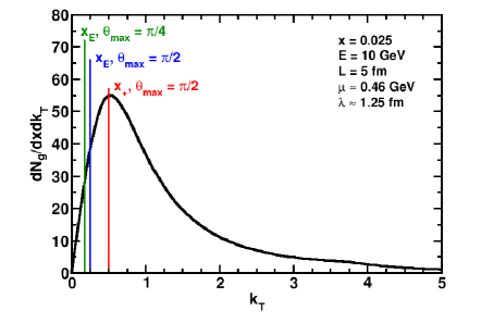
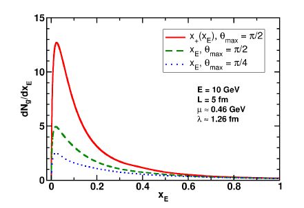
The different physical pictures have made it difficult to consistently fix parameters for a direct comparison of models. However a recent comparison was performed by applying the GLV, AMY and ASW (both MS and SH) formalisms to a “brick” of QGP matter of fixed length [150]. A comparison of medium-induced gluon emission spectra and nuclear suppression factors as a function of for each of the different models are shown in Figs. 2.27 and 2.28 respectively.
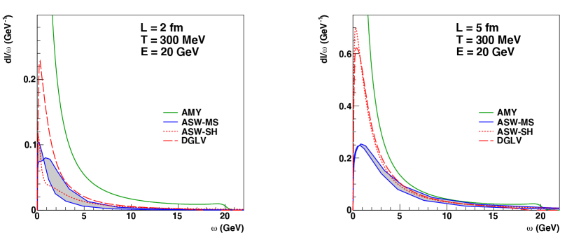
Depending on the formalism, the quenching mechanism is sensitive to the system size as well as some combination of the intensive parameters , and , which provide information about the microscopic medium dynamics. The soft multiple scattering approximation is only sensitive to , which is defined as the mean-squared momentum transfer per unit length,
| (2.86) |
where is the differential elastic scattering rate for a hard parton in a thermal medium. This behaves as at high temperatures, but is screened at low temperatures by , given by Eq. 2.76. The form,
| (2.87) |
interpolates smoothly between these limits [150], and the number density has been introduced [179],
| (2.88) |
The leading coefficient is the ratio of Riemann zeta function values, . The value of is given by,
| (2.89) |
where is the largest transverse momentum transfer allowed in the elastic scatterings and is a function of and in principle the parton energy as well. This introduces a logarithmic dependence of on , which is an effect of approximating the collision integral in the evaluation of the elastic scattering rate. This value is sometimes taken as although may be more appropriate [180]. The value,
| (2.90) |
and calculated below, is a commonly used, energy independent expression and is equivalent to omitting the logarithmic variation of . These estimates can differ by up to 40% for large parton energies.
The opacity can be calculated as
| (2.91) |
which in turn, determines . However the form of the scattering rate here is slightly different than the one given in Eq. 2.87, and is chosen to be consistent with the model used in the opacity expansion framework [150]. This gives
| (2.92) |
which is consistent with Eq. 2.90.

Motivated by new experimental capabilities at the LHC, extensions of energy loss calculations to full jets have recently been made [181, 182, 183]. These function by expressing the differential jet cross section as,
| (2.93) |
where is the probability a jet will lose a fraction of its energy. The Jacobian relates the initial and final parton by , and is given by
| (2.94) |
The factor is the fraction of the emitted radiation above and inside the jet cone defined by ,
| (2.95) |
While this form still only considers the energy loss of the leading parton, it does take into account the extent to which radiated energy is not lost, but only redistributed within the jet. Furthermore, it facilitates the usage of NLO and NPDF effects in the pQCD calculation of the unmodified jet cross section, . The factorization of medium-induced radiation from the production cross section, which is used in Eq. 2.93 has been proven in the context of an effective theory. This uses Soft Collinear Effective Theory (SCET) techniques to decouple the hard and soft components of the gluon fields and has been shown to reproduce the GLV expression when expanded to first order in opacity [184]. This factorization is also applicable to multi-jet systems, allowing calculations of differential energy loss in dijet systems. Calculations of the inclusive jet suppression factor and dijet asymmetry in this framework are shown in Figs. 2.29 and 2.30, respectively.
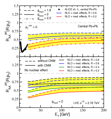
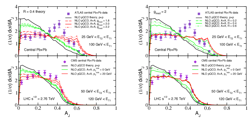
The AdS/CFT correspondence principle was discussed in Section 2.4.4, in the context of estimating the shear viscosity. Similar techniques have also been applied to study the energy loss of fast partons. While many of these results have focused on the specific case of heavy quarks [185, 186, 187, 188], some work has been done to provide an estimate of [189, 190, 191]. These results agree qualitatively with the range of estimates from experiment.
2.6 Relativistic Heavy Ion Collisions: RHIC to LHC
With the commencement of the RHIC program, many of the speculated features of heavy ion collisions became experimentally accessible. The collective behavior of the system can be studied by measuring the angular distribution of particles, . As discussed previously, in the absence of hydrodynamical expansion, this distribution is expected to be isotropic. The anisotropy can be quantified by considering the Fourier decomposition of the distribution,
| (2.96) |
where are the event plane angles, and describe the magnitude of the modulation. In all but the most central collisions, the direction of the impact parameter vector between the nuclear centers defines a reaction plane. The overlap region is ellipsoidal and symmetric about this reaction plane. The second Fourier coefficient, , is an observable with sensitivity to how the initial-state anisotropy is converted to the final-state particle distribution, a phenomenon known as elliptic flow. Measurements from the RHIC program show that the elliptic flow, in particular the magnitude of the azimuthal modulation of particles as a function of their , is well-described by ideal, relativistic hydrodynamics. The near-vanishing viscosity indicates that the system is strongly coupled. This came as a surprise when compared to the prediction of asymptotically free quarks and gluons and which has led to monikers such as the strongly-coupled QGP (sQGP) and “the perfect liquid” applied to the medium created at RHIC. Since early RHIC results, significant advances have been made in the formulation and numerical implementation of viscous hydrodynamics. RHIC and LHC values are compared with a recent viscous hydrodynamical calculation in Fig. 2.31.
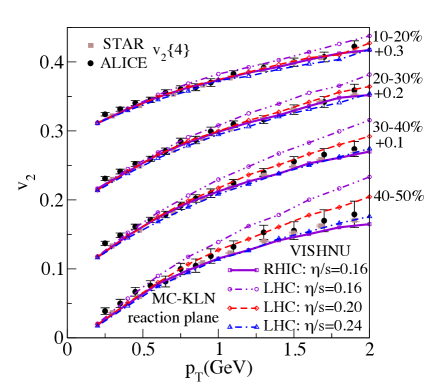
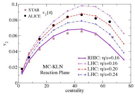
More recently, it was recognized that the event-by-event fluctuations in collision geometry could drive higher flow harmonics. These provide additional information about the initial-state geometry and may be able to provide additional constraints on the hydrodynamical formulation or the value of the shear viscosity. The first six harmonics as measured by ATLAS [195] are shown in Fig. 2.32.
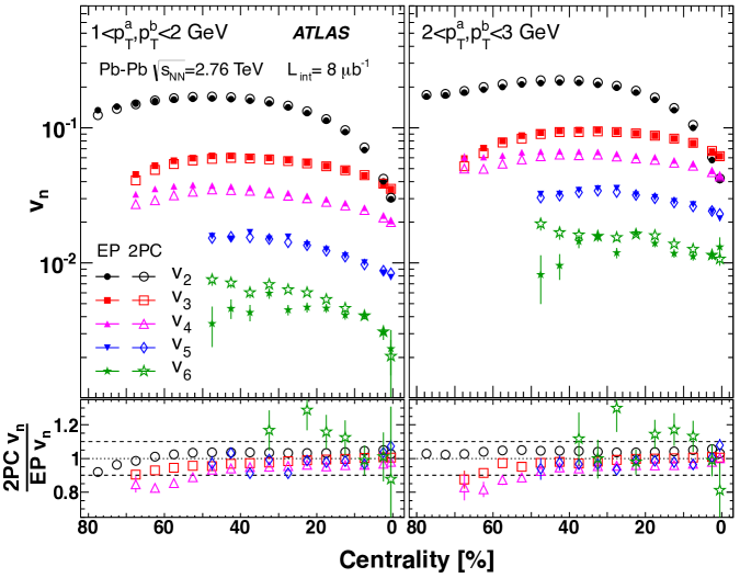
2.6.1 Hard Processes
Indirect experimental evidence for jet quenching was first established by two important measurements. The single hadron spectrum was found to be heavily suppressed at high- in central collisions [196, 197, 198, 199]. Furthermore, the away-side correlation in the dihadron angular distribution was found to be heavily modified in central Au+Au relative to [200, Adler2005ee, 201]. These two measurements provide slightly different handles on the phenomenon as the former is an inclusive measurement of the total effect of the suppression on the spectrum. The latter provides a differential measurement of the quenching as it is sensitive to the quenching of one jet relative to another.
The interpretation of these observations as evidence for quenching was further supported by results from the d+Au run which established a critical baseline. The lack of suppression at high- [202, 203] combined with the unmodified dihadron correlation indicated that modification of the NPDFs was not responsible for the observations in Au+Au. Subsequent measurements of the direct photon were consistent with no suppression and provided further systematic control on the quenching effects [204].
The degree of suppression is typically quantified by the nuclear modification factor, ,
| (2.97) |
A summary of the measurements from PHENIX is shown in Fig. 2.33. These results established that the production of high- particles is strongly influenced by the produced medium in heavy ion collisions.
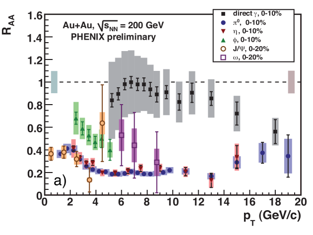
However, the single particle measurements (with the exception of the photon), are limited in their utility. The medium effects involve a high momentum parton, not a final-state hadron. Thus single particle observables can only be connected to the process of interest through a fragmentation function. This necessity forces the interpretation of the results in the context of strict factorization between the medium effects and fragmentation. While this factorization may ultimately prove to be an appropriate assumption, it is desirable and more objective to work in a more general paradigm for the jet-medium interaction, namely one that does not enforce strict separation between medium effects and the jet fragmentation. Furthermore, the single hadron observables are only linked to the parton level quantities in an average sense; there is no guarantee that the highest energy hadron in an event came from the leading jet, or the jet that suffered the least energy loss. This limitation is removed if per-jet fragmentation distribution is eliminated from the observable.
It is less restrictive, although more experimentally challenging, to construct observables from fully reconstructed jets. These quantities provide direct sensitivity to quenching effects. Furthermore, the possibility of using jets as input objects into physics analyses opens many new possibilities, which will be discussed in detail in Chapter 7. Measurements of full jets at RHIC have been attempted, but are limited by a number of factors and as of this time no such measurement has been published. The main complication is due to the production rates of jets that are easily detectable above the medium background. Measurements are further constrained by the limited acceptance of the PHENIX and STAR detectors. Although highly collimated, particles from jets can still be distributed over a substantial angular range. Typical sizes for the cone radii and parameters in the sequential clustering algorithms used in experiments are on the order of . Thus larger acceptance detectors are preferred for jet measurements.
Many of these issues are not present at the LHC, in particular the ATLAS experiment, discussed at length in Chapter 3. At these high energies, the first Pb+Pb run was at TeV, the rate for producing jets well above the background from the underlying event is much higher; the differential single jet inclusive cross section nb for 100 GeV jets in collisions at these energies. Furthermore, the high quality calorimetry covering 10 units in enables precise measurements of jets and their properties.
Chapter 3 Experimental Setup
3.1 The Large Hadron Collider
The Large Hadron Collider (LHC) is a particle accelerator at CERN outside of Geneva, Switzerland. Although it was primarily designed to collide protons, the machine is also capable of colliding heavy ions. This program began in November 2010 with the first lead ion collisions.
The LHC machine [206] was constructed using the tunnel originally used for the LEP experiment. It consists of two parallel beam lines circulating particles in opposite directions, intersecting at designated interaction points (IPs). The ring is 26.7 km in circumference and contains eight arcs and straight sections. The particle orbits are primarily controlled by the 1232 dipole magnets, while strong transverse focusing of the beam constituents is maintained by alternating field gradients supplied by 392 quadrupole magnets. Almost all of these devices use superconducting NbTi cabling operating in a cryogenic system maintained by superfluid He II at 1.9 K.
ions are extracted from a source and processed by a sequence of injection chain elements before being injected into the LHC. This sequence is shown in Fig. 3.1 consists of: Linac3, the Low Energy Ion Ring (LEIR), the Proton Synchrotron (PS) and the Super Proton Synchrotron (SPS). In this process the ions are stripped of electrons, squeezed into longitudinal bunches via the application of a radio frequency electric field (RF) and accelerated to a beam energy of 177 GeV per nucleon.
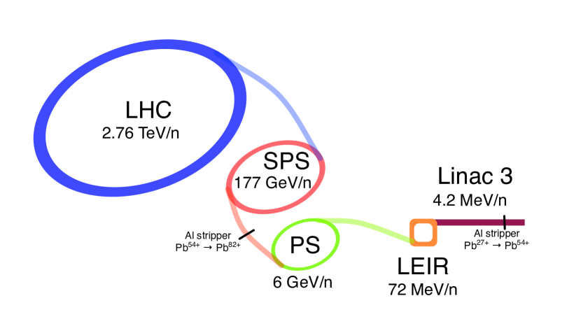
3.1.1 Performance and Luminosity
The most important factor in determining a collider’s performance is the luminosity. The instantaneous luminosity of a particle beam, , is the flux of scattering particles per unit area per unit time. For a process with cross section the interaction rate is given by
| (3.1) |
Therefore to enhance the rate of rare processes, it is a design goal of an accelerator to maximize this quantity. The colliding beams consist of bunches of ions with densities and . Along the beam direction, , the bunches can be organized into various patterns according to an injection scheme in which each colliding bunch pair collides regularly with frequency . In the transverse direction, the beams have profiles characterized by and . For bunches the instantaneous luminosity can be computed via
| (3.2) |
The beam’s transverse focusing is controlled by applying alternating gradient fields forcing the beam to converge. The transverse motion of single particles within the beam is then a sinusoid with an envelope modulated by the beta-function,
| (3.3) |
where and are integrals of motion, describing the area and angle of an ellipse in the phase space (, ) inhabited by beam particles [30]. To maximize luminosity in the neighborhood of the interaction zones, the beams are squeezed in the transverse direction by focusing magnets [207]. The squeezing is parabolic in the longitudinal displacement and is controlled by the parameter
| (3.4) |
In addition to , the other parameter affecting luminosity is the emittance, . In the absence of beam losses, the phase space ellipse has fixed area . For a beam with a Gaussian transverse profile, the emittance is the area containing one standard deviation :
| (3.5) |
In terms of these parameters, the luminosity can be expressed as
| (3.6) |
The longitudinal beam structure is governed by the bunch injection scheme [208]. The SPS is capable of injecting proton bunches at 25 ns spacing or 40 MHz into the LHC, corresponding to a total 2,808 bunch crossing slots (BCIDs). As of yet, this design limitation has not been reached. The end of the 2011 proton run injected 1380 bunches, 1331 of which were brought into collision for a luminosity of . The 2010 Pb ion run saw a maximum luminosity of corresponding 121 bunches per beam with 113 colliding bunches and a 500 ns bunch spacing shown in Fig. 3.2.
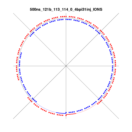
For the entire 2010 Pb ion run, the LHC delivered a total integrated luminosity of 9.69 . This quantity, as well as the total integrated luminosity recorded by the ATLAS detector as a function of time is shown in Fig. 3.3. Although not analyzed here, the 2011 Pb ion run recorded a total integrated luminosity of approximately 140 .
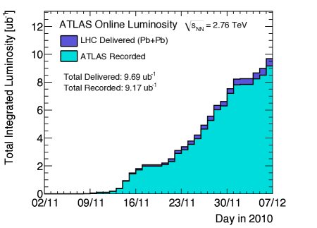
.
In addition to the discrete bunch structure, RF cavities are used to focus the bunches in the longitudinal direction. The 400 MHz oscillating field causes particles to clump together around the ring in each of the 35640 RF buckets. Superimposing the RF structure with the injection bunch spacing causes 10 RF buckets to be associated with each BCID. Ideally all particles in the injected bunch are forced into a single RF bucket, however a few stray particles become trapped in adjacent buckets as indicated in Fig. 3.4. Collisions among these particles, called satellite bunches, will appear out of time with the LHC clock in discrete 2.5 ns intervals.
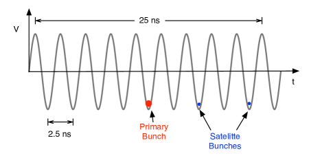
3.2 ATLAS Overview
The ATLAS experiment is a multi-purpose particle detector situated at interaction point 1 (IP1) of the ATLAS ring [209]. It is forward-backward symmetric covering the full 2 in azimuth. Charged particle tracking is provided by the inner detector, covering , immersed in a 2 T solenoidal magnetic field which is shown in Fig. 3.6. Energy measurements are provided by a combination of electromagnetic and hadronic calorimeters covering enclosing the inner detector. A dedicated muon spectrometer is positioned beyond the calorimeter utilizing a toroidal field maintained by a barrel and two end-cap toroidal magnets. This system allows muon measurements over the range utilizing a variety of subsystems.Forward detectors such as the Zero Degree Calorimeter () and Minimum Bias Trigger Scintillators () provide minimum bias event triggering and event selection capabilities. A graphical representation of ATLAS highlighting the various subsystems is shown in Fig. 3.5.
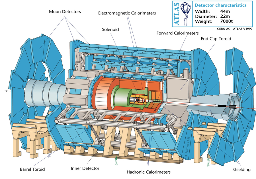
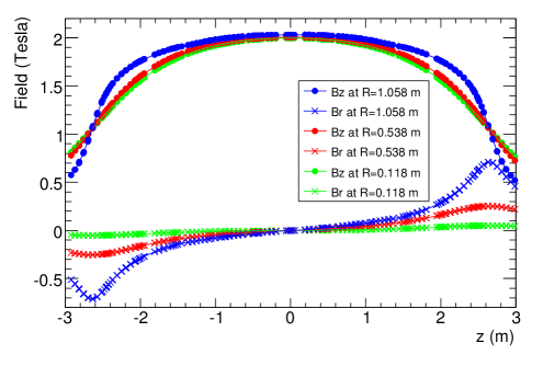
3.3 Trigger
A trigger is a combination of hardware and software elements designed to select which collision candidates are recorded by the data acquisition (DAQ) system. When few colliding bunches are circulating in the machine, a simple requirement that the given pair of bunches is intended to collide in the filling scheme is the most basic criterion for triggering. However this is insufficient as many of the recorded events may contain no real collisions or detector signals from beam and cosmic backgrounds. Additionally, at higher luminosity the DAQ typically cannot record events at this rate and a trigger selection must be employed to ensure that only events with desired physics signals are recorded. In general, implementing a sophisticated trigger strategy to solve this problem is a significant experimental effort, requiring multiple triggers sensitive to different physics signals as well as using prescales to reduce the rate of less interesting triggers relative to the rarer ones. However, the luminosity of the 2010 ion run was low enough that a set of minimum bias trigger items could be selected without need for prescale.
The ATLAS trigger system is composed of trigger items on three different levels. The Level 1 (L1) trigger is entirely hardware-based. In addition to the normal data readout path, detectors integrated into L1 have parallel paths for data readout, often involving coarser and faster signal sums. The specialized trigger signals are sent to the Central Trigger Processor (CTP), which combines the information into a set of L1 bits. The other two levels Level 2 (L2) and Event Filter (EF) are both software based and are collectively referred to as the High Level Trigger (HLT). L1 regions of interest (ROIs) are used to seed algorithms run as part of L2. Finally, L2 items feed full scan EF algorithms, which use higher level detector signals from the offline readout path and are not constrained to the L1 ROIs. A trigger chain is defined as an EF item that is seeded by various L1 and L2 items. Multiple chains can be seeded by the same L1 and L2 items and prescales can be applied at any of the three levels. Trigger chains are grouped together by type to form data streams; an event is recorded and reconstructed if it has been selected by one or more of its chains after all prescales have been applied.
During the 2010 ion run, a single minimum bias stream,
physics_bulk, was used for physics analyses. While some chains
using HLT items were used for efficiency and background studies, this
stream was primarily composed of raw L1 items passed through the HLT
without prescale.
3.4 Calorimetry
The ATLAS calorimeter system is composed of electromagnetic and hadronic calorimetry using sampling calorimeters based on two distinct technologies: liquid Argon (LAr) and scintillating tiles. The coverage and segmentation of each subsystem is summarized in table 3.1. Energies of particles well above the ionization regime are measured by a sampling technique. Electromagnetic and hadronic showers are initiated when the particle strikes an absorber. The details of these showering mechanism are discussed in Sections 3.4.1 and 3.4.2 respectively. As the showers develop the energy of the incident particle is increasingly spread among an ensemble of particles of lower energy. An active material is placed behind the absorber which collects some fraction of energy of the lower energy particles, either through ionization (LAr) or scintillation (tile). Alternating layers of absorber and active material are placed in succession and the shower-sampling is repeated. A pictorial representation of the different calorimeters and the sampling of the different shower types is shown in Fig. 3.7.
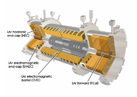
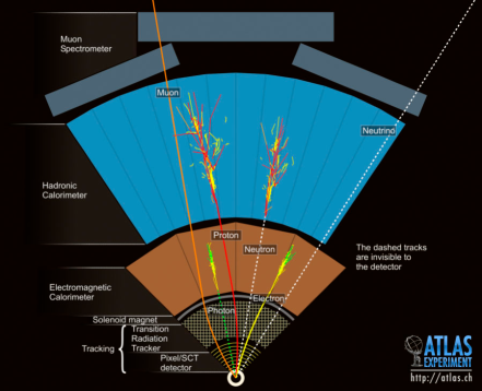
| Type | Sub-detector | Absorber | Layer | -range | Channels | |
| LAr | Barrel Presampler | None | 1 | 7808 | ||
| EM Barrel | Steel | 1 | 57216 | |||
| 2 | 28672 | |||||
| 3 | 13824 | |||||
| End-cap Presampler | None | 1 | 1536 | |||
| EM End-cap | Steel | 1 | - | 28544 | ||
| 2 | 23424 | |||||
| 3 | 10240 | |||||
| Hadronic End-cap | Copper | 1 | 3008 | |||
| 2 | 2624 | |||||
| FCal | Copper | 1 | 1008 | |||
| Tungsten | 2 | 500 | ||||
| 3 | 254 | |||||
| Tile | Tile Barrel | Steel | 1 | 5760 | ||
| 2 | ||||||
| 3 | ||||||
| Tile Extended | Steel | 1 | 4092 | |||
| 2 | ||||||
| 3 |
The EM barrel and end-cap sub-detectors constitute the first sampling layers over the central portion of the detector () and possess fine segmentation for high-precision measurements. Both of these sub-detectors use sheets of steel-reinforced lead as absorbers, between 1.53 and 1.7 mm thick, folded into an accordion shape as shown in Fig. 3.8.
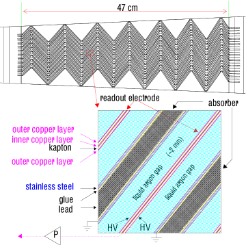
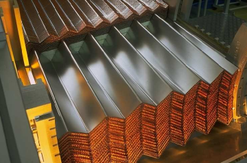
The sheets are stacked and interleaved with readout electrodes positioned in the middle of the gaps on honeycomb spacers. The barrel consists of two separate half-barrels ( and ) each containing 1024 sheets with the accordion pattern extending radially, stacked to form cylinders covering full in azimuth. The cylinders each have a length 3.2 m with inner and outer diameters of 2.8 m and 4 m respectively. The end-caps consist of two co-axial wheels, of inner and outer radii 330 mm and 2098 mm respectively, composed stacked of absorber sheets and interspaced electrodes with the accordion pattern running parallel to the beam direction.
The absorber structures are sealed inside cryostats filled with liquid Argon at 88.5 K. The absorbers initiate electromagnetic showers, with the lower energy particles in these showers producing ionization electrons in the LAr. In addition to the sampling layers, separate “presampler” layers of LAr are placed in front of the first barrel and end-cap layers. These modules allow for the collection of energy from electromagnetic showers that start early due to the material in front of the calorimeter. The amount of material, as indicated by the number of radiation lengths as a function of is shown in Fig. 3.9. The sharp peaking in the upper left figure is caused by the edge of the cryostat, which projects to a narrow range in .
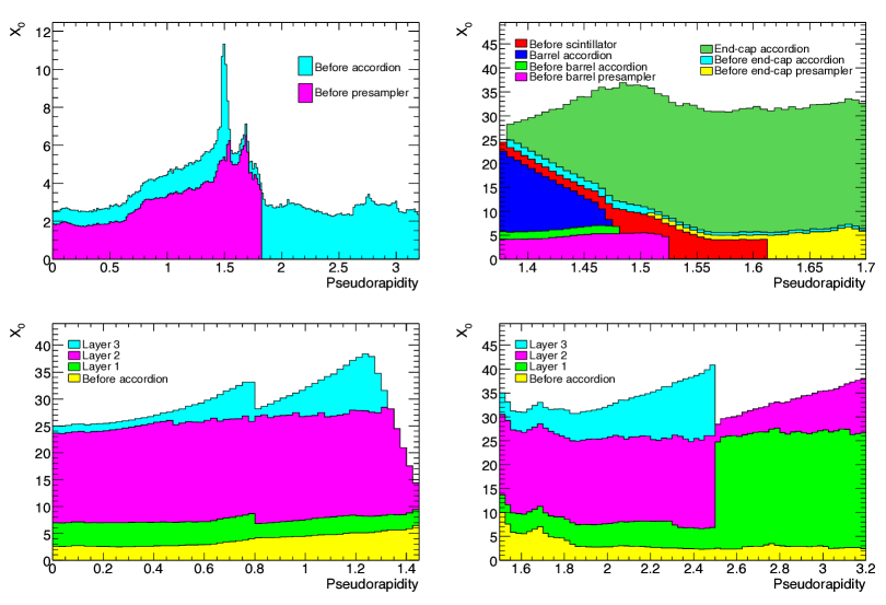
The electrodes are held at high voltage and collect the drifting ionization electrons as a signal. This signal is processed by cold electronics mounted inside the cryostat. These signals are passed out of the cryostat through dedicated signal feed-throughs to a front-end crate, which provides signal amplification, pulse shaping and analog-to-digital conversion (ADC), and output with optical links to the main DAQ system. The front-end electronics possess an independent readout path for the L1 trigger where analog sums of adjacent cells are taken before ADC. The trigger readout possesses a dedicated readout path. This has the benefit that a correction for “dead cells” in the offline readout due to a failure of the optical link is possible using the coarser trigger information (dead OTX correction).
The high luminosity requires short drift times ( ns). In the barrel the geometry allows for gaps of fixed size between the absorber and electrodes, 2.1 mm, which corresponds to an operating voltage of 2000 V. The end-cap geometry does not allow this, thus the applied voltage is -dependent, varying from 1000-2500 V. The signal current is proportional to the electron drift velocity, which is both a function of the applied voltage and the temperature of the cryogenic liquid, thus the temperature and purity are monitored closely. Measurements of the drift velocity performed using cosmic muons prior to the start of LHC operations are shown in Fig 3.10; good uniformity was found in the measured drift velocities at the operating voltages and temperature [210].
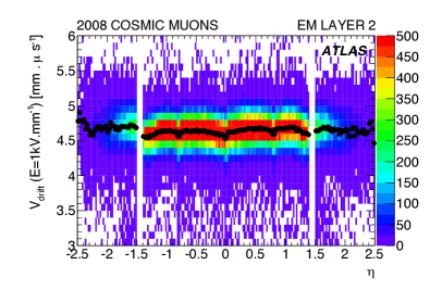
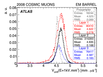
The hadronic end-cap calorimeter (HEC) also uses liquid Argon as an active medium, however it uses copper plates to increase the number of interaction lengths and thus functions as a hadronic calorimeter. The end-caps are symmetric, and each side is composed of a front and rear wheel module. The copper plates are oriented perpendicular to the beam axis and there are 24 plates each 25 mm thick in the front wheel modules, and 16 plates each 50 mm thick in the rear modules. The wheels each have a front plate of half the nominal plate thickness, 12.5 and 25 mm respectively. The LAr gaps are fixed at 8.5 mm, and are divided by three electrodes into four drift zones of 1.8 mm. The readout cells are defined by pads which are etched on the surfaces of the electrodes. A schematic drawing of the HEC including dimensions is shown in Fig. 3.11.

The final element of LAr-based technology are the FCal modules. These modules cover and are divided into three longitudinal layers. All three layers use absorber plates perpendicular to the beam axis. These plates have tubes bored into them in the beam direction. Each tube is filled with a rod containing a coaxial cathode and anode electrodes. The space between electrodes is filled with LAr forming a small, 0.249 mm gap. The first layer is an electromagnetic calorimeter and uses copper for the absorber. The second and third layers have similar geometry but are constructed from 2.35 cm copper front and back plates which support tungsten rods. The region in between rods is filled by filleted tungsten slugs to maximize the number of interaction lengths. The layout of the absorber matrix for the first FCal layer is shown in the left panel of Fig. 3.12. The FCal, HEC and EM end-cap modules are all situated inside the same cryostat with the positioning of the FCal modules shown on the right of Fig. 3.12.
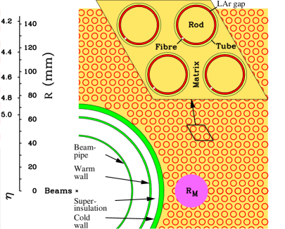
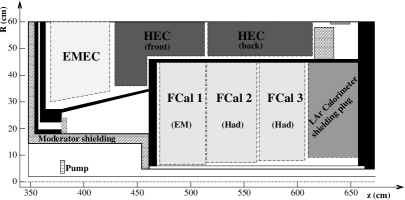
The remainder of the calorimetry in ATLAS is provided by the tile system, which uses alternating steel plates and polystyrene scintillating tiles. This system is composed of central () and extended () barrel sections. Each consists of 64 self-supporting, wedge-shaped modules, partitioned in azimuth. A diagram of one such tile drawer is shown in Fig. 3.13. Scintillation light is collected in wavelength-shifting fibers and fed to photomultiplier tubes mounted at the edge of the modules. The fibers are grouped to provide three radial sampling depths of thicknesses 1.5, 4.1 and 1.8 interaction lengths (at ). In addition to the nominal central and extended barrel regions, a series of tile scintillators are placed in the geometrically-irregular gap regions between the cryostat. The segmentation of the tile modules and positioning of the gap scintillators is shown in Fig. 3.14.


A summary of the amount of hadronic sampling as a function of calorimeter layer an , as indicated by the number of nuclear interaction lengths (see Section 3.4.2) is shown in Fig. 3.15.
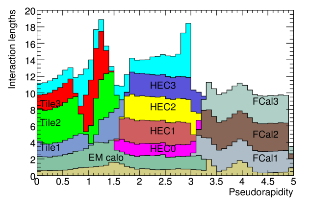
3.4.1 Electromagnetic Showers
In the low to moderate energy regime, energy loss is described by the Bethe formula which describes the interaction of charged particles and material through the excitation and ionization of atoms. Typically the lost energy is extractable by collection of ionization electrons or scintillation light. Above some energy, called the critical energy , the energy loss is dominated by bremsstrahlung radiation, or pair production in the case of photons. The length scale associated with the energy loss rate is known as the radiation length, , and describes the mean distance over which a particle will lose of its initial energy through radiation. This quantity depends on the detailed structure of the material including the atomic charge screening effects on the bremsstrahlung cross section as well as the density of scattering centers. It has approximate dependence on the nuclear charge and atomic number of the material as . The photon pair-production cross section is controlled by physics at a similar scale, and at high energies is approximately of the mean free path for a photon to travel before pair production.
When a high energy electron or photon enters material, the induced radiation or splitting results in the initial energy being distributed among two lower energy particles. These two particles lose energy through the same mechanism, and this process continues developing an ensemble of particles among which the initial energy is shared. This process is known as an electromagnetic shower or cascade. Once particles in this ensemble become lower than the critical energy, they no longer contribute to the shower’s development, which eventually dies off. The longitudinal development of the shower can be described by a simple model. Since each step in the shower development is binary, after a number of interaction lengths the shower will contain approximately particles, and the average energy is , where is the incident electron energy. The system should freeze out when the mean energy is of order , which corresponds to a shower depth of
| (3.7) |
More sophisticated models describe the average evolution by a gamma distribution, which allows for more parameters in describing the medium dependence of the shower. In the transverse direction, the shower width is well described by the Molière radius, , where MeV.
3.4.2 Hadronic Showers
Electrons and photons, as well as particles that decay into them such as the , are measured exclusively through electromagnetic showers. Occasionally will undergo quasi-elastic charge exchange, resulting in an electromagnetically detectable . The bremsstrahlung rate for heavier particles is suppressed by the large particle masses. Energy measurements of other particles typically occurs through hadronic showers, which are considerably more complicated than their electromagnetic counterparts. The exceptions are muons and neutrinos, neither of which interact hadronically. The former are typically detected as minimum ionizing particles and often require a dedicated muon tracking system to measure. The neutrino energy can be inferred from so-called missing variables in hermetic detectors.
Inelastic collisions of hadrons incident on atomic nuclei result in a wide range of byproducts resulting in large fluctuations in the measurable energy in a hadronic shower. As the shower develops some fraction of energy becomes electromagnetically visible in the form of produced ’s, which start their own electromagnetic showers. While some of the collisional debris may be detectable through ionization, many of the struck nuclei become fragmented resulting in spallation neutrons, which are difficult to detect. Although some neutrons thermalize producing photons which can be measured through late neutron capture, much of the shower energy in spallation neutrons and nuclear recoil cannot be collected. A material’s ability to initiate hadronic showers and appear opaque to hadronically interacting matter is given by the nuclear interaction length , which describes the mean free path for undergoing inelastic hadronic interactions in a medium.
Hadronic showers typically develop a substantial electromagnetic component. Thus hadronic calorimeters have separate responses to electromagnetic and hadronic processes. If these responses are significantly different, an effect known as non-compensation, fluctuations in the electromagnetic/hadronic composition in a shower will significantly increase the energy resolution and cause a response that is not linear in the incident particle energy. Both of these features are undesirable and represent key constraints when designing a hadronic calorimeter. Typically these features are minimized by decreasing the electromagnetic sensitivity (lower ) while increasing the hadronic (higher ).
3.5 Minimum Bias Trigger Scintillators
The ATLAS Minimum Bias Trigger Scintillators (MBTS) detector is used to both select collision candidates online and reject background events in offline event selection. This detector is composed of 32 modules, each a 2 cm thick polystyrene scintillator embedded with wavelength shifting fibers for readout. The modules are located m from the detector center with a total coverage of and in azimuth. Each side (A and C) contains 16 modules in two groups in : , . Each group contains 8 wedges which together span the full azimuth.
A trigger readout is implemented by applying a leading-edge
discriminator to the signal pulse sending a hit to the CTP for each of
the 32 modules that is over a threshold. Additional L1 items are built
from these bits including the coincidence triggers,
MBTS_N_N, which are fired if or more modules fired on each of the A and C sides.
Aside from the L1 trigger, the MBTS is primarily used offline for timing. From the pulse sampling, a time measurement relative to the LHC clock can be determined for each side. The MBTS can be used to reject out-of-time signals corresponding to non-collision background or collisions between satellite bunches.
3.6 Zero Degree Calorimeters
Positioned m from the interaction points are the ATLAS Zero Degree Calorimeters (ZDC). The detector measures neutral particles with , in particular spectator neutrons in heavy ion collisions; all charged nuclear fragments are swept away by magnetic fields before reaching the ZDC. Each side contains four rectangular modules, the first of which is an electromagnetic module with finer readouts. Each module contains 11 plates perpendicular to the beam direction made from a combination of tungsten and stainless steel absorbers. Between the plates are mm quartz strips. Hadronic showers of incident particles are initiated by the absorber. Čerenkov light from the showering particles is produced in the quartz and fed through air light-guides into photomultiplier tubes situated on top of the detector. Some of the modules contain specialized quartz rods to provide position measurements, although this aspect of the detector capability is not used in minimum bias event selection for heavy ion collisions.
For the 2010 ion run, the ZDC was used primarily as a minimum bias
trigger. Each side is capable of producing a L1 trigger signal by passing the
analog channel sums through a discriminator to the CTP. The
coincidence trigger, ZDC_A_C,
is a logical AND of the one-sided triggers,
ZDC_A and ZDC_C. The requirement
of a single neutron on both sides is effective in rejecting against
photo-nuclear collisions, which are typically asymmetric and are a
large background to the most peripheral collisions.
3.7 Inner Detector
The ATLAS inner detector occupies a cylindrical volume around the detector center spanning mm in the direction and 1150 mm in radius. Space-point measurements are provided by three separate sub-detectors over the radial extent of the system, each divided into barrel and end-cap modules. A slice of the detector in the plane showing the various components is shown in Fig. 3.16. Additional figures showing perspective views of the inner detector system in the barrel and end-cap region are shown in Fig. 3.17.
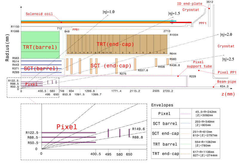
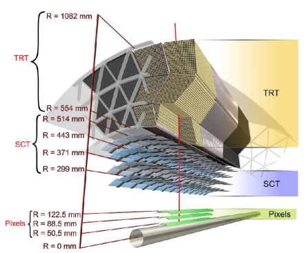
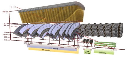
The silicon pixel detector is composed of three cylindrical layers beginning at a radial distance of 50.5 mm and three end-cap disks per side. It contains 1744 identical pixel sensors which are 250 thick oxygenated n-type wafers with readout pixels on the -implanted side of the detector. Each sensor contains 47232 pixels for a total of approximately 80 million readout channels (the total number of channels is reduced by the ganging of adjacent pixels on front-end chips). The pixels have a nominal size of 50 in and 400 in providing measurements with intrinsic inaccuracies of 10 in for all modules and 115 in and for the barrel and disk modules respectively.
The silicon microstrip detector (SCT) consists of four cylindrical layers and nine disks per side each composed of small angle stereo strips positioned beyond the pixel detector. The barrel covers the radial region mm, and mm. The end-cap modules are positioned mm and mm. The strips are composed of two 6.4 cm daisy-chained sensors, thick, with a strip pitch of 80 . In the barrel these strips are oriented parallel to the beam direction, measuring , while in the end-caps they are trapezoidal wedges and are oriented radially.
The Transition Radiation Tracker (TRT) is the outermost component of the tracking system. The barrel spans radial region mm and mm. The end-cap wheels span mm, positioned between mm. It is composed of polymide drift tubes, 4 mm in diameter and 71.2 cm in length. The tube wall is composed of two 35 multi-layer films. The cathode is a 0.2 Al film on the inner surface. The anode wires are 31 gold-plated tungsten, positioned at the nominal center of the tube. To ensure stable operation the wires are required to have an offset with respect to the tube center of less than 300 . The tubes are filled with a gas mixture of approximately 70% Xe, 27% and 3% , held slightly over-pressure. Photons from transition radiation of high energy electrons can be distinguished from normal ionization tracking signals on a per tube basis using separate high and low thresholds on the readout electronics. The wires are divided into three sections. They are read out at each end, with an inefficient center section of approximately 2 cm, which contains a mid-wire support structure. The TRT barrel is composed of 73 layers of tubes oriented along the beam direction, while the end-caps consist of 160 tube planes. Charged tracks will cross at least 36 tubes except in the barrel/end-cap transition region () where this minimum drops to 22.
Chapter 4 Jet Reconstruction
4.1 Subtraction
For a calorimetric measurement, the input to the jet reconstruction procedure is the measured distribution, which contains both the jet signal and contributions from the underlying event,
| (4.1) |
The magnitude of the underlying event can vary over several orders of magnitude depending on the collision geometry, thus an accurate procedure requires that a background estimation be performed on an event-by-event basis. Correlations in the underlying event, specifically , must be incorporated into the subtraction procedure as well. The background energy density is estimated by
| (4.2) |
where is the event plane angle and is the average density taken over the full in azimuth in strips of constant with width 0.1. To account for variation of detector response in the different longitudinal sampling layers, the background determination and subtraction is performed per layer.
The possibility exists for the jets to bias the determination of . If a jet’s energy is included in the background calculation, the background is overestimated, resulting in an over-subtraction being applied to the jet. This effect, called the self-energy bias, will bias the jet energy after subtraction by approximately 10% and will distort the as well. To address this, the jet reconstruction used in this analysis employed an iterative procedure where jets were reconstructed and identified as jet seeds. was constructed with the seeds excluded from the determination of . This reduced the bias in the background and the subtracted jets. These jets were then be used as seeds to iterate the procedure, by constructing new estimates of and .
4.1.1 Seeds
In clustering algorithms, such as anti-, the entire distribution is tessellated by reconstructed jets. While some of these jets likely correspond to a true jet signal, the clustering of many of the background jets is due to the underlying event. If a set of criteria can be chosen to partition the full set of jets output by the reconstruction into one that characterizes the background distribution and one that does not, the latter can be used as jet seeds. A simple threshold cannot be used to define the seeds at this stage since the subtraction has not yet been performed. For the first step in the iterative procedure, a discriminant was constructed by considering the distribution of tower ’s inside a jet and taking the ratio of the maximum and mean of this distribution:
| (4.3) |
A cut of identifies jets with a dense core spanning a few calorimeter towers, which are typical of the true signal. This requirement fails when calorimeter noise allows the denominator of the discriminant to become arbitrarily small resulting in a large discriminant even when the distribution maximum is also small. To prevent this from occurring, a threshold on was be applied in conjunction with a minimum requirement on the tower distribution maximum or mean. This cut was taken to be a minimum value of 3 GeV.
In subsequent stages of the iteration procedure the jets that were the output of the previous iteration step were reused as seeds. Since these jets had already been subtracted, an cut of 25 GeV could be applied to define the seeds. In addition to these jets, track jets with were also added to the list of seeds.
4.1.2 Background Determination
The average density was computed by considering all calorimeter cells and calculating an average transverse energy density per cell. For a sampling layer the average is defined as
| (4.4) |
The average was only taken over cells that are in the same pseudorapidity bin as and are not associated with a seed. In the discriminant-based approach, the seed-associated cells were defined as the constituents of the jets that pass the discriminant cut. In all other cases they were defined as being within of a seed position as shown in Fig. 4.1. This exclusion radius was used regardless of the value used in the anti- algorithm. The -dependent demodulation factors were required since the average was not performed over the full range and thus elliptic flow effects do not cancel.
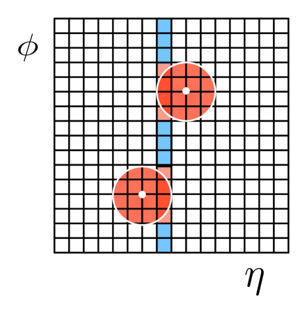
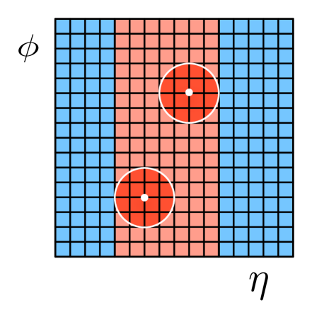
4.1.3 Elliptic Flow Correction
The event plane angle was determined using the first layer of the FCal using the same procedure as in Refs. [211]. This angle was then used to determine the per calorimeter sampling layer ,
| (4.5) |
where the brackets denote an weighted average over all cells in layer .
As was the case for , it is possible for the jet signal to bias the . This effect is worsened by the fact dijet signals have the same symmetry as the flow modulation.
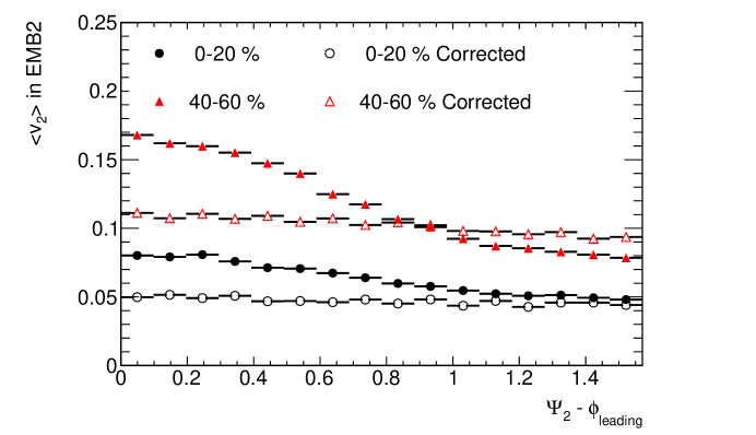
Jet seeds can be used to exclude regions containing potential jets from the averaging and eliminating the bias. However, excluding small regions around a seed as described in Section 4.1.2 cannot be done. In a strip of constant , excluding some of the cells from the full azimuthal interval will cause an anti-bias; the for events where jets are aligned with the event plane will be reduced. To prevent this overcompensation, the entire interval was considered to be biased by the jet. Such intervals were flagged using the jet seeds and excluded from the average in Eq. 4.5. This exclusion is shown schematically in Fig. 4.1. The effect of jets on as measured in the second sampling layer of the barrel electromagnetic calorimeter in MC simulations is shown in Fig. 4.2. Without excluding jets from the determination (solid markers), the calculated is larger in events where the leading jet is aligned with the event plane. This bias is removed once the jet seeds are excluded from the calculation as indicated by the open markers in the figure.
4.1.4 Subtraction
Once the background and flow parameters were determined, a subtraction was applied at the cell level. For a cell at position in layer , the corrected was determined from the raw via
| (4.6) |
Each cell was considered as a massless four-vector using the after subtraction. The jet’s kinematics were set as the four-vector sum of the constituent cells.
This subtraction was applied to all cells except dead cells that receive no correction from neighboring cells or the associated trigger tower. The latter correction was only applied if the trigger tower was above a 2 GeV noise threshold. Thus for the purposes of subtraction, dead cells eligible for this correction were checked event-by-event.
4.1.5 Calibration
Jet collections were constructed using two different calibration schemes. The EM+JES scheme uses the cell energies, after subtraction, at the EM scale and applies a final, multiplicative calibration factor to the jet energy to calibrate to the full hadronic scale. In the GCW scheme, a calibration is done at the cell level, which designed to minimize variation in hadronic response to jets. However, a multiplicative calibration factor is still required to account for the mean hadronic response. In this scheme the determination and subtraction use calibrated cell energies111The was determined using cells at the electromagnetic scale. For jets using the GCW scheme, the in Eq. 4.6 was first demodulated by the flow weight , calibrated and then re-weighted by the same factor.. The GCW also accounts for energy lost due to material in the cryostat by calculating a correction using the energy deposition in the third electromagnetic and first hadronic sampling layers after subtraction.
After subtraction the multiplicative jet energy calibration factor was applied to correct for the overall jet energy. The factors depend on both the jet’s energy and , and different constants are used for the GCW and EM+JES schemes. The numerical inversion constants were developed specifically for heavy ion jets and are discussed in Section 4.3.2.
4.1.6 Track Jets
Jets reconstructed with charged particles provide an invaluable cross-check on the calorimetric jets. The anti- algorithm with was run using charged particles as input. Instead of performing a subtraction, particles were required to have a minimum of 4 GeV to be included in a track jet in addition to the following track selection requirements, where impact parameter variables are defined with respect to the primary reconstructed vertex:
-
•
,
-
•
,
-
•
,
-
•
.
4.1.7 Jet Collections
With the exception of the track jets, all the results presented here use jet collections obtained with the iterative method using a single iteration step applied to both the background and flow. Seeds were constructed by running anti- with . The discriminant procedure was used to determine the background, and the initial values were used with this background to produce subtracted, flow corrected jets. The list of seeds for the iteration step was constructed from jets with and all track jets with . This list of seeds was used to define new background and values. These were used to construct iterated jet collections with four different values of : and . For each of these values of , two versions of the collections exist corresponding to the two calibration schemes: GCW and EM+JES. The 25 GeV cut defining the seeds was chosen based on the observation that the fake rate for jets above this is not too high to cause biases in the subtraction when a fake jet is used as a seed.
4.2 Monte Carlo Sample
The studies presented here use a Monte Carlo sample of minimum bias HIJING Pb+Pb events with embedded PYTHIA events at . Events from both generators were produced and the detector response to each event was independently simulated using a full GEANT [212, 213] description of the ATLAS detector [214]. The signals were combined during the digitization stage and then reconstructed as a combined event. For each HIJING sample a set of PYTHIA samples (referred to as J samples) was produced, each with a fixed range set on the and in the PYTHIA hard scattering. A single HIJING event was overlaid on an event from each of the different J samples, with no reuse of HIJING events within a J sample, i.e. . The different J samples were then combined using a cross-section weighting obtained from PYTHIA to build a combined sample with good counting statistics over a wide range of jet . The definitions of these samples and the associated cross sections are shown in Table 4.1.
| J | [GeV] | [GeV] | [] | |
|---|---|---|---|---|
| 1 | 17 | 35 | 157000 | |
| 2 | 35 | 70 | 7090 | |
| 3 | 70 | 140 | 258 | |
| 4 | 140 | 280 | 5 | .85 |
| 5 | 280 | 560 | 0 | .0612 |
As HIJING does not contain a mechanism for simulating elliptic flow, an afterburner was applied to modulate the azimuthal angles of the HIJING particles using a , and centrality-dependent parametrization of existing data [215]. Samples used in this study use a parametrization derived from 2010 Pb+Pb data at the LHC.
The goal of the embedding procedure is to study the combined effect of the underlying event and detector response on the jet signal. Truth jets were constructed from the generator-level particle content of the PYTHIA event only. These jets were then compared to the output of offline jet reconstruction to extract metrics of jet performance and information for correcting measurements for these effects.
The HIJING events themselves contain jet production at a rate consistent with binary scaling. A per-event jet yield for these jets is shown in Fig. 4.3. A subtlety arises in the embedding procedure when the particles from a hard scattering in the HIJING background overlap with those from the PYTHIA jets. The reconstructed jet signal will contain contributions from both PYTHIA and HIJING, however the matching truth information will only contain the jet energy from PYTHIA.
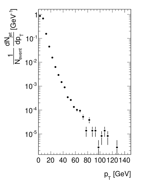
While this problem affects truth jets of all energies, it is most easily seen in samples of J1 events where the PYTHIA jets have relatively modest energies. In a high-statistics sample, some of the HIJING events contain jets in excess of 100 GeV, resulting in many events where these jets overlap in - with a PYTHIA jet of much lower of order 10 GeV. Given the large weight of the J1 sample, without correcting for the HIJING contamination the most probable way to get a 100 GeV jet in the full study is through this mechanism. The associations between 10 GeV truth jets and 100 GeV reconstructed jets significantly distort studies of jet performance and the response matrix.
Running jet reconstruction on the HIJING particles leads to many of the challenges of background separation/subtraction that are faced in the full offline reconstruction. Uncertainties in identifying the truth jet energy would reduce the effectiveness of any performance studies. It is possible for multiple hard scatterings in the same heavy ion event to produce jets that overlap in the calorimeter. This is likely to be a small effect and would be best addressed by extending the embedding process to multiple overlapping PYTHIA jets, where the identification of truth energy is clear. The procedure used in this study to remove HIJING contamination is to run the anti- algorithm with on HIJING particles with . The energies of these jets were not used in the performance study, but instead any PYTHIA jet found within of a HIJING jet with is removed from the sample. The fraction of jets removed during this procedure in each and centrality bin is recorded and the final distributions are re-weighted by the inverse of this fraction.
The overlaid events must have the same vertex position at the generator level. This constraint requires that multiple samples be produced at different, fixed vertex positions, rather than the usual case of a single production sampling a continuous distribution. The positions of the samples, and the relative number of events produced per position is shown in Fig. 4.4. The vertex and positions were fixed for all samples to match the mean beam-spot position from the 2010 Pb+Pb run. A total of one million HIJING events were generated along with one million PYTHIA events in each of the five different J samples.
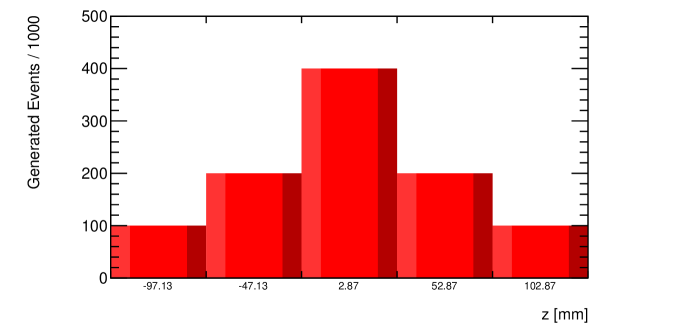
4.3 Corrections
4.3.1 Self and Mutual Energy Biases
As mentioned in Section 4.1, a self-energy bias can occur when there is an incomplete match between the jets used as seeds and the final jets after iteration. To address this possibility, a variable was computed during reconstruction assuming the jet failed to be excluded from the background and thus biased its own energy subtraction. At the analysis stage, any jet not associated with a seed has its energy corrected. The iteration step reduces this problem considerably as all high energy jets () are excluded from the background and are unaffected. However for jets around this threshold the self-energy bias correction must be included.
The above procedure assumes the bias is binary: either a jet is biased or it is not. However, if the region around a seed does not contain the entire geometric area spanned by the jet, a differential bias can occur determined by the region of non-overlap. Additionally, jets that are not excluded from the background may cause over-subtraction in another jet in the same interval (mutual energy bias). The underlying event can produce calorimetric signals that appear as jets, but are in fact uncorrelated with hard particle production in the event. The contribution and systematic removal of such fake jets is discussed extensively in Section 4.3.3. The set of jets capable of biasing the background (or being biased themselves) must be consistent with the definition of fake jets. The energy bias correction was applied by considering the constituent towers of jets that pass fake rejection and calculating a bias for each strip in by summing the energies of those towers unassociated with a seed (). Each jet was then corrected at the constituent level for biases introduced by constituents of other jets that were not excluded by the seeds.
4.3.2 Numerical Inversion
Numerical inversion is a method to derive the and -dependent jet calibration. The method described below follows the procedure used in the jet energy scale determination used in jet measurements [216]. The main motivation to derive calibration constants for heavy ion jet reconstruction is that no such constants exist at this time for , and in . Additionally, some aspects of the reconstruction differ slightly between and Pb+Pb, most notably the issue of noise suppression. Thus the application of numerical inversion constants derived using heavy ion jets will be more appropriate than the existing and constants.
The calibration constants are derived using 60-80% peripheral events from PYTHIA+HIJING Monte Carlo samples described in Section 4.2. The basic quantity used in the derivation of the calibration constants is the response,
| (4.7) |
where is reconstructed at the EM scale and is the of the truth jet. The response was evaluated for all calorimeter jets which match a truth jet and track jet simultaneously. The matching condition required a separation of between the calorimeter jet axis and truth (track) jet axis. The calorimeter jet was required to be isolated, that is no other calorimeter jet within must be present ( is the parameter of the anti- algorithm).
The response was evaluated in 12 bins in pseudorapidity of the reconstructed calorimeter jet, , on the interval and 23 bins in the . For in bin , the quantities and were determined using a Gaussian fit and a statistical mean respectively. The set of points was fit with the function:
| (4.8) |
where is between 1 and 4. The actual value of is optimized to provide the best . A separate set of points and fit parameters were determined for each . The calibrated , , was then defined by
| (4.9) |
An example of the response as a function of is shown in Fig. 4.5, where the response is well described by the functional form of Eq. 4.8. A similar level of agreement is found for all bins. Figure 4.6 shows the dependence of the jet energy scale after applying the derived calibration constants. A detailed closure test is discussed in Section 4.4.1.
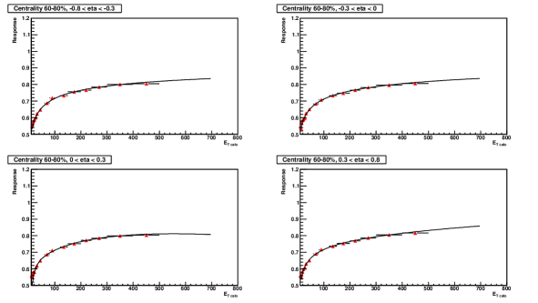
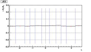
4.3.3 Fake Rejection
Fluctuations of the underlying event that are unassociated with a hard scattering can create localized high regions in the calorimeter that may be reconstructed as jets. In the most central collisions these fake jets contribute significantly to the jet spectrum up to 80 GeV. As most of this signal is caused by accumulated energy from soft particles, requiring a physics signature consistent with hard particle production in the neighborhood of a jet can reject against this background. To minimize the contamination of the sample of reconstructed jets by fake jets different methods for fake jet identification and rejection were studied. The general requirement of a coincidence of the reconstructed calorimeter jet with the track jet or an electromagnetic cluster was found to be efficient at removing fakes without a severe impact on the overall efficiency. For the duration of this thesis, the fake rejection, unless otherwise noted, is defined as the requirement that a jet have a track jet or EM cluster with within of the jet’s axis. The effectiveness of this rejection procedure is discussed in Section 4.3.4.
Fig. 4.7 compares the jet reconstruction efficiency in central (0-10%) and peripheral (60-80%) collisions in two cases: before applying the fake rejection (solid symbols) and after applying the fake rejection (open symbols). The overall jet reconstruction efficiency is reduced by the fake rejection requirement but still remains near 50% for 30 GeV jets.
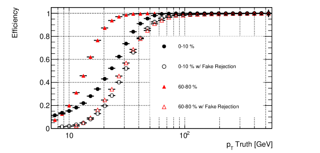
Corrections derived from MC for efficiency loss due to fake rejection (moving from solid to open markers in Fig. 4.7) will be sensitive to how accurately the MC describes this effect. The accuracy of the MC result can be checked in the data by comparing the ratio of the spectrum after fake rejection to the total spectrum, which shows the survival fraction of jets at a given that pass the rejection criteria. This comparison must be made with caution and only in regions where a significant fake rate in the data is not expected because the embedded MC sample is not expected to accurately describe the fake rate. Since every event in the embedded MC sample contains a PYTHIA hard scattering event the relative rates of true jets (from the PYTHIA signal) to fake jets (from soft particles in the HIJING background) will not be correct. A HIJING-only sample is required for an evaluation of the absolute fake rate, a procedure which is discussed in Section 4.3.4.
A comparison of the survival fraction222It should be emphasized that this distribution is not trivially related to the efficiency shown in Fig. 4.7. One important difference is that the efficiency is shown as a function of of the truth jets. The survival fraction shown in Fig. 4.8 is evaluated as a function of reconstructed , since the data is being used, which has the effects of upward feeding from finite resolution. in data and MC is shown in Fig. 4.8. The fake rate is expected to be negligible in peripheral collisions and good agreement is seen between data and MC in the survival fraction in the 60-80% centrality bin (red markers). This indicates that efficiency loss of true jets due to the fake rejection requirement is well described by the MC, and that a MC-based correction for this effect is appropriate. For GeV, fakes are also expected to be a negligible contribution to the spectrum in the 0-10% bin. In this region, where the efficiency approaches its asymptotic value, the agreement between data and MC is better than 0.5%.
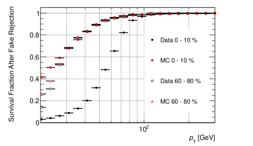
High- tracks and clusters are expected to be associated with particles within jets, however it is possible for reconstructed jets to pass fake jet rejection due to combinatoric overlap between the jet and the track jet/cluster. This combinatoric rate is the mechanism by which fake jets pass rejection, and a data to MC comparison of this rate can be used to construct a more accurate estimate of the fake rate in data from the residual fake rate obtained from the MC study. This rate was evaluated by considering the distribution of all track jets, electrons and photons in an event with respect to a jet’s axis. To simplify geometric effects from splitting of nearby jets, only isolated jets were considered. These jets were required to be the highest jet in a cone about their axes. In the MC sample jets were additionally forced to match a truth jet () and be isolated from any HIJING jets ( for GeV). Comparisons between the different objects (track jets, electrons and photons) and between data and MC are shown for jets in central and peripheral collisions in Fig. 4.9.
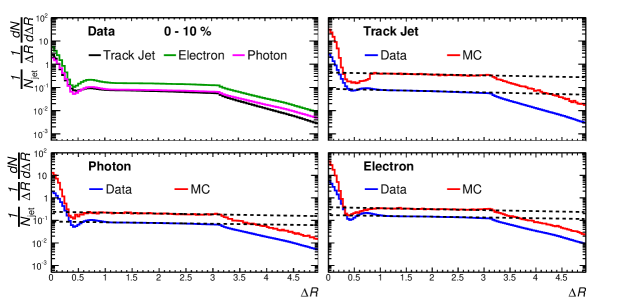
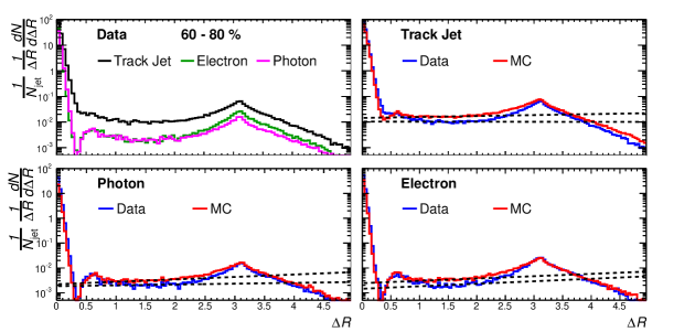
The distributions show strong correlation for matches at small with a more diffuse peak at associated with the dijet structure of the events. The remainder of the distribution is expected to be determined purely by geometry, thus the trivial geometric enhancement has been removed by dividing by . With this effect removed, the matching rate is expected to be constant away from the jet and dijet peaks, which is estimated by the background extrapolations shown in the figures. These distributions have been normalized per jet, such that the background distribution integrated over the matching region can be interpreted as a per jet probability of combinatoric match, , via
| (4.10) |
where the quantity in parentheses is estimated from fitting the distribution in the region and extrapolating underneath the correlation peak at . Estimates of these probabilities in central collisions are compared for data and MC in Fig. 4.10.
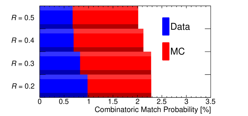
The rates are nominally independent of , which is expected as the jet definition does not explicitly enter into the matching. The MC are higher than the data by factor of 2-3, which is qualitatively consistent with observed single particle suppression factors, caused by a phenomenon (quenching) present in the data but not the MC.
4.3.4 Residual Fake Rate
The residual per-event rate of fake jets (underlying event fluctuations) after fake rejection was determined from an analysis of a HIJING-only MC sample. Each reconstructed jet passing the fake rejection criteria but not within of a HIJING jet with GeV was considered a fake jet. The residual fake rate is defined as the ratio of these unmatched jets to the total number of reconstructed jets passing fake rejection and is a function of .
Unlike the truth jet reconstruction in PYTHIA-embedded events, the HIJING truth jet reconstruction was run with a GeV cut on the input particles to the reconstruction algorithm. Because of this, a hard-scattered parton may fragment in a way that is not reconstructed by the HIJING truth jet reconstruction as a jet with GeV. A jet reconstructed from these fragments will fail to match a truth jet causing the fake rate calculation to come out anomalously high. Therefore, it is necessary to calculate the truth jet reconstruction efficiency of a truth jet if the reconstruction had been performed with a GeV cut on the constituents. After correcting the fraction of jets that match to a HIJING truth jet by the truth jet reconstruction efficiency, the difference between the efficiency corrected rate and the full jet rate is the residual fake rate.
Only reconstructed jets within are considered for the residual fake rate analysis. Reconstructed jets that pass fake jet rejection are corrected for the self-energy bias as described in Section 4.3.1. The analysis is repeated for three different fake jet rejection schemes:
-
•
GeV track jet or GeV cluster within ,
-
•
GeV track jet or GeV cluster within ,
-
•
GeV track jet within .
To calculate the truth jet reconstruction efficiency resulting from the GeV constituent cut, a subset of the J1 and J2 PYTHIA-embedded Monte Carlo samples were used ( events mm only). PYTHIA truth jets were matched to reconstructed jets with . To determine if this truth jet would be reconstructed by the definition used in the HIJING only sample, the summed energy of PYTHIA truth particles with GeV within a radius of the truth jet axis was required to be greater than 10 GeV. Because GeV truth jets in the underlying HIJING event can combinatorially overlap with a PYTHIA truth jet, the truth jet reconstruction efficiency is actually higher for a PYTHIA truth jet at the same in central than in peripheral collisions. To include this effect, the of HIJING jets within of the truth jet’s associated reconstructed jet’s axis was also added the PYTHIA truth particle sum.
As previously noted, a significantly higher- hard scattering in HIJING may combinatorially overlap with an embedded PYTHIA truth jet. To prevent such scenarios from contaminating the efficiency calculation, the same HIJING contamination removal condition is applied. Even with this constraint, there are cases when a HIJING jet overlaps a PYTHIA jet. However, this effect of such overlaps is not obvious due to truth jet reconstruction inefficiency. Therefore, jets with GeV (about - times the RMS energy from underlying event fluctuations in central events for jets) were also excluded. In central events and peripheral events, and of jets, respectively, are properly isolated from contamination from HIJING hard scatterings.
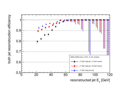
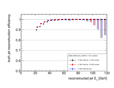
To determine the efficiency in each bin, the J samples were combined in a weighted average,
| (4.11) |
where is the number of generator events in that centrality selection, is the generator cross-section for the J sample given in Table 4.1 and is the number of jets at the given reconstructed . Figure 4.11 shows the truth jet reconstruction efficiency in the most central and most peripheral events for each of the three fake jet rejection schemes.
The truth jet reconstruction efficiency was then used to determine the residual fake rate in central events from the HIJING-only data set. Reconstructed jets that pass fake rejection were tested to see if they match to a HIJING hard scattering. This is accomplished by considering the summed of all HIJING truth jets with GeV within of the reconstructed jet. Reconstructed jets where this sum exceeds 10 GeV were considered a match, with the unmatched yield defined as the remainder after the matched is subtracted from the total. The total per-event yield in the 0-10% centrality bin along with the matched and unmatched is shown on the left side of Fig. 4.12. The matched distribution was then corrected for the truth jet inefficiency and the difference between the total yield and this corrected, matched yield provides an estimate of the absolute fake rate is shown on the right side of Fig. 4.12.
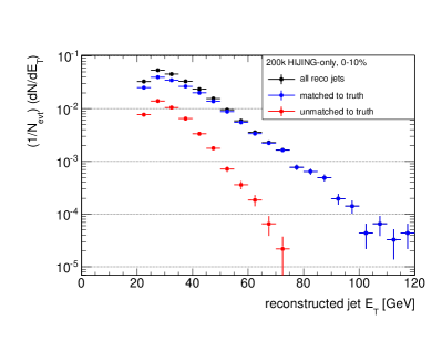
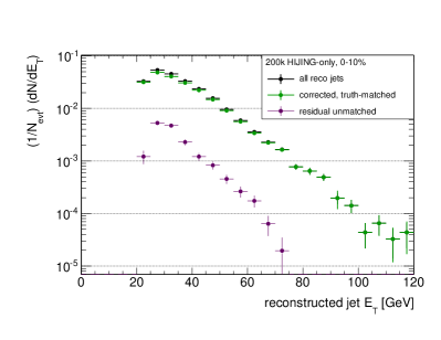
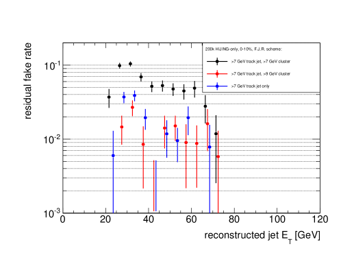
For reconstructed jet at a given , the probability that this jet is unmatched defines the residual fake rate. This quantity was calculated by normalizing corrected, unmatched yield by the total yield, and is shown in Fig. 4.13 for the three fake jet rejection schemes in 0-10% centrality bin. For GeV, this rate is -% for the fake jet rejection scheme used in this analysis: matching to track jet or cluster with GeV. This rate drops to -% for the schemes with stricter requirements, although these were not used in the jet spectrum analysis due to their effect on the efficiency. If a fake jet passes the rejection it is due to a combinatoric overlap between an underlying event fluctuation reconstructed as a jet and a single track or cluster also from the underlying event. The rate for this behavior was estimated in the previous section, and the MC rate was found to exceed that of the data by a factor of 2-3. The residual fake rate extracted from the MC should be reduced by this factor when describing data. Thus the absolute fake rate is estimated to be 2-3% for GeV in the most central 10% of events.
4.4 Performance
To evaluate jet performance using the Monte Carlo samples, “truth” jets were matched to reconstructed jets by requiring an angular separation between truth and reconstructed jet, . If multiple reconstructed jets were matched to a truth jet, the reconstructed jet with the smallest was selected. For the results presented in this section, performance plots are presented for all jets with using the EM+JES calibration scheme.
4.4.1 Jet Energy Scale
For each matched truth jet, the difference,
| (4.12) |
was calculated. The distribution of was then evaluated as functions of , and centrality. To evaluate the jet energy scale (JES) as a function of the distributions were each fit by a Gaussian. At low ( GeV for jets) the distributions are affected by a truncation of reconstructed jet at 10 GeV. For finite bin size in , this results in a distortion of the shape of the distribution at low . Therefore the distribution was fit in the region which is unaffected by this truncation. Above 50 GeV the effect of the truncation is minimal as indicated in the left plot of Fig. LABEL:fig:JESFitExample.
The evaluation of the JES as a function of is shown on Fig. 4.14. Upper plots and lower two plots of Fig. 4.14 compare the JES for different jet definitions in the 0-10% and 60-80% centrality bins. Lower right plot then shows the JES in seven centrality bins for jets. At low the accuracy of the evaluation of the JES is limited by precision of fitting of the truncated Gaussian distribution. In these cases, to the left of vertical lines are provided in the figures, an upper limit on the JES (as indicated by the arrows on the error bars) is estimated. The difference between central and peripheral collisions is at most 2% for collections. The one percent non-closure in jets is due to the fact that the derivation of numerical inversion constants requires isolated jets, but the JES evaluation includes non-isolated jets as well.
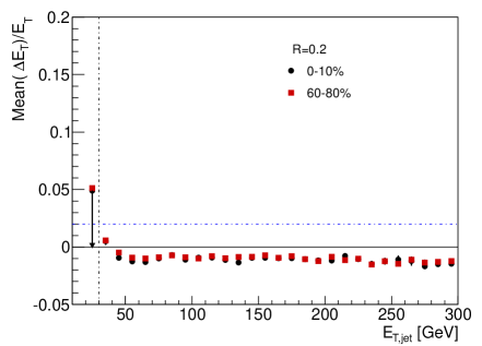
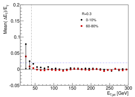
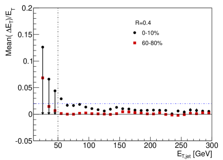
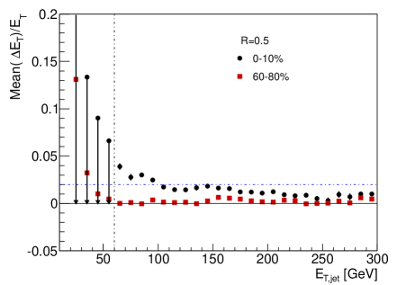
Comparison of JES as a function of is shown in Fig. 4.15. The JES as a function of was evaluated by calculating the mean of the distribution of all reconstructed jets corresponding to truth jets with GeV.
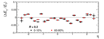
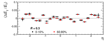
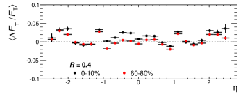
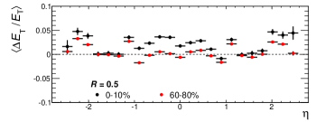
The behavior of the JES as a function of can be summarized by fitting the distribution with a linear function:
| (4.13) |
The term is typically small, and the constant term represents the non-closure in the JES calibration. The values of this constant term for all centralities and values are shown in Fig. 4.16.
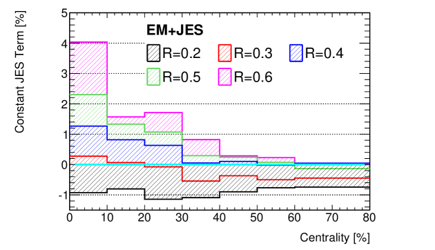
4.4.2 Jet Energy Resolution
The jet energy resolution (JER) can be defined using the width of the Gaussian fit discussed in the previous section. Figure 4.17 shows the evaluation of JER in different bins of centrality and for different jet definitions. The JER increases both with increasing centrality and increasing jet radius. Validation studies of the JER using data are presented in Sec. 5.3.2.
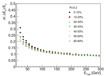
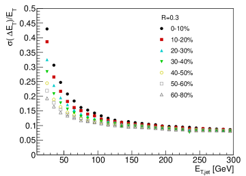
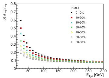
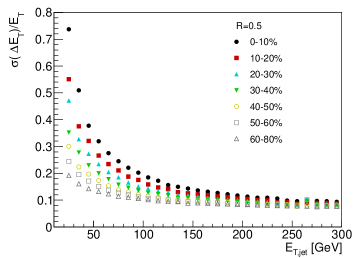
An alternative definition of the JER uses the standard deviation of the distribution in bins of ,i.e.
| (4.14) |
Figure 4.18 shows the evaluation of the difference between the two JER definitions for jets and 0-10% central collisions. The Gaussian-fit JER is slightly smaller for GeV, which can be attributed to the asymmetric distribution resulting from the minimum threshold on reconstructed jets.
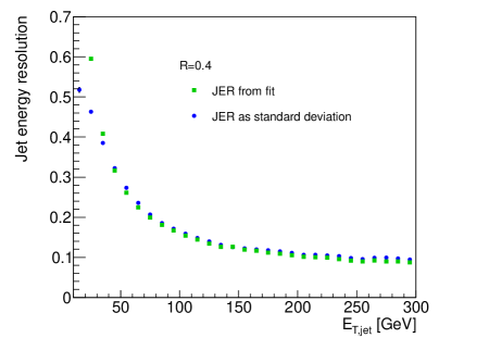
4.4.3 Jet Reconstruction Efficiency
The jet reconstruction efficiency is defined as:
| (4.15) |
where and are the total number of truth jets and number of truth jets with a matching reconstructed jet in a given bin. The reconstruction efficiencies are shown in Fig 4.19. The and jet reconstruction efficiency reaches 95% by 60 GeV in the most central (0-10%) Pb+Pb collisions and 30 GeV in the most peripheral (60-80%) collisions. The last 5% increase in the efficiency takes place near 70 GeV for all centrality bins. For the and jets, the efficiency reaches 95% below 40 GeV for all collision centralities and is approximately above 50 GeV.


Figure 4.20 shows the jet reconstruction efficiency a function of for jets with . The smaller radii have saturated the efficiency turn on at this energy and show no variation. The and jets are not full efficient at this energy in the most central collisions and show a slight reduction in the efficiency between the barrel () and end-cap () regions.


Chapter 5 Data Analysis
5.1 Data Set
The data presented in the following section were recorded by ATLAS during the 2010 Pb+Pb run. During this run a total integrated luminosity of approximately was recorded and determined to be of sufficient quality for physics analysis. An additional sample of was recorded with the solenoidal magnetic field turned off; this data set will not be considered here.
The events analyzed were required to satisfy a set of minimum bias event selection criteria. These were chosen to require a physics signature consistent with an inelastic Pb+Pb collision. Additional conditions were imposed to reject photo-nuclear and non-collision background. The requirements were as follows:
-
1.
The event was recorded because it satisfied a minimum bias trigger. Events were required to have fired one of the following triggers after prescale and veto (events dropped due to dead time):
-
•
MBTS coincidence:
L1_MBTS_N_N, where N 1, 2, 3 or 4. -
•
ZDC coincidence:
L1_ZDC_A_CorL1_ZDC_AND.
-
•
-
2.
Good MBTS timing. The A and C side times were required to satisfy ns.
-
3.
ZDC coincidence. Regardless of how the trigger selection was made the event must have one of the ZDC coincidence triggers before prescale, a logical
ORbetweenL1_ZDC_A_CandL1_ZCD_AND. This was found to be essential for rejecting against photo-nuclear events. -
4.
A good reconstructed vertex.
Applying these event selection criteria, combined with selecting luminosity blocks consistent with stable running and detector operation resulted in a sample of 50 million events. These event selection criteria were used in all heavy ion analyses within ATLAS using the 2010 data.
5.2 Centrality Determination
The centrality determination used the total transverse energy as measured by the ATLAS FCal system, . The pseudorapidity coverage of this system, , is well separated from the central region of the detector, meaning that specific, centrality-dependent physics processes will not bias the centrality determination. The was found to be strongly correlated with the total energy deposited in the rest of the calorimeter, making it an excellent indicator of global event activity. The correlation between total energy in the electromagnetic barrel, , and is shown in Fig. 5.1.
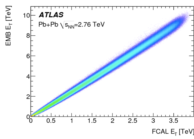
The minimum bias distribution has a distribution typical of other centrality variables such as the total number of charged particles, as well as Glauber quantities and . This distribution is shown in Fig. 5.2.
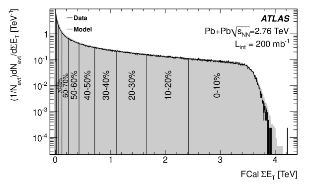
A two-component model as given by Eq. 2.67 was used to fit this distribution. An additional check was performed by taking an n-fold convolution of the distribution based on a Glauber MC, which agreed well. A complete analysis of the 2010 centrality determination is given in Ref. [217]. The minimum bias event selection cuts were determined to introduce a 2% inefficiency, almost entirely from the MBTS timing cut. The distribution of as a function of is shown in Fig. 5.3.
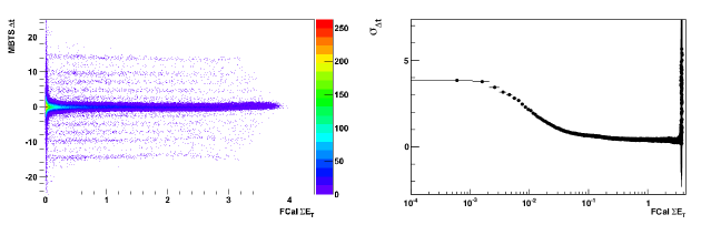
Under the assumption of 98% efficiency, the distribution was divided into 10% intervals, except for the range 60-100%, which was divided into two intervals of 20% each, in the fashion discussed in Section 2.5.1. In each bin the corresponding events in the Glauber MC were averaged to obtain and . These values are shown in Table 5.1. This table also shows the ratios of factors, which are used directly in the determination. The uncertainties were evaluated by considering the effects of varying ingredients into the Glauber calculation such as the nucleon-nucleon cross section, the two Woods-Saxon parameters as well as a 2% variation of the inefficiency. The errors on in different centrality bins are correlated so the uncertainties on were constructed appropriately.
| Centrality [%] | [TeV] | ||||||||||||||||
|---|---|---|---|---|---|---|---|---|---|---|---|---|---|---|---|---|---|
| low | high | low | high | ||||||||||||||
| 0 | 10 | 2. | 423 | 1500. | 63 | 114. | 8 | 56. | 7 | 11. | 4 | 356. | 2 | 2. | 5 | ||
| 10 | 20 | 1. | 661 | 2. | 423 | 923. | 29 | 68. | 0 | 34. | 9 | 10. | 5 | 261. | 4 | 3. | 6 |
| 20 | 30 | 1. | 116 | 1. | 661 | 559. | 02 | 40. | 5 | 21. | 1 | 9. | 4 | 186. | 7 | 3. | 8 |
| 30 | 40 | 0. | 716 | 1. | 116 | 322. | 26 | 23. | 9 | 12. | 2 | 7. | 9 | 129. | 3 | 3. | 8 |
| 40 | 50 | 0. | 430 | 0. | 716 | 173. | 11 | 14. | 1 | 6. | 5 | 6. | 1 | 85. | 6 | 3. | 6 |
| 50 | 60 | 0. | 239 | 0. | 430 | 85. | 07 | 8. | 4 | 3. | 2 | 3. | 8 | 53. | 0 | 3. | 1 |
| 60 | 80 | 0. | 053 | 0. | 239 | 26. | 47 | 3. | 5 | 22. | 6 | 2. | 1 | ||||
5.3 Validation
5.3.1 Jet Energy Scale
A number of studies were performed using data to check the accuracy of the jet energy scale calibration procedure which was derived from MC.
5.3.1.1 EM+JES vs GCW Comparison
The jet reconstruction was performed with both the EM+JES and GCW calibration schemes. A comparison of spectra using each of these schemes is shown for jets in Fig. 5.4. In general good agreement is found between both schemes.
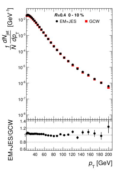
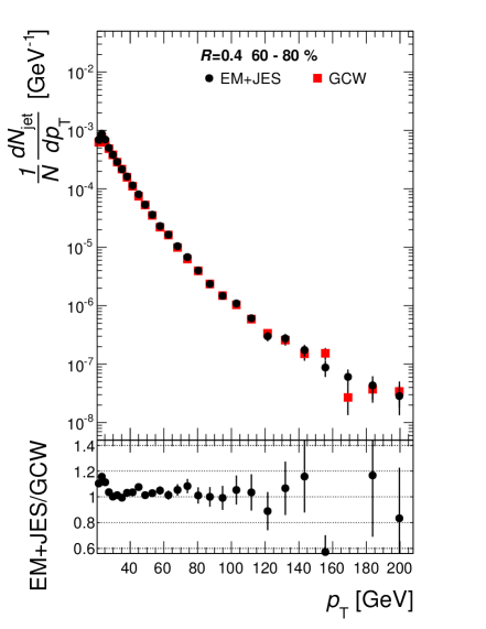
5.3.1.2 Track Jet Matching
One of the methods to validate the performance of the jet finding, in particular the jet energy scale, is to match the calorimeter jets to track jets and compare their momenta. Such a comparison can be done both in the MC and in the data. Calorimeter jets were matched to track jets with GeV, with a matching requirement of between the calorimeter and track jet axes. Fig. 5.5 shows the calorimeter jet as a function of a corresponding track jet both for the data and MC for the 0-10% and 60-80% centralities. For calorimeter jets with GeV,the mean calorimeter jet , , was computed as a function of the track jet and is overlaid on top of the two-dimensional distributions.
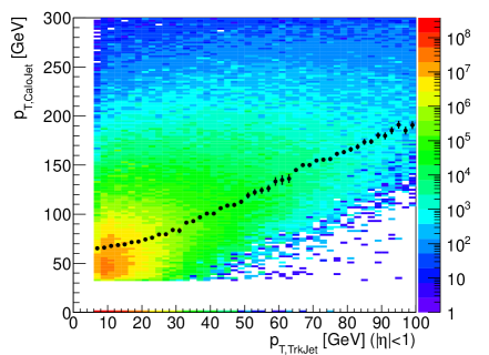
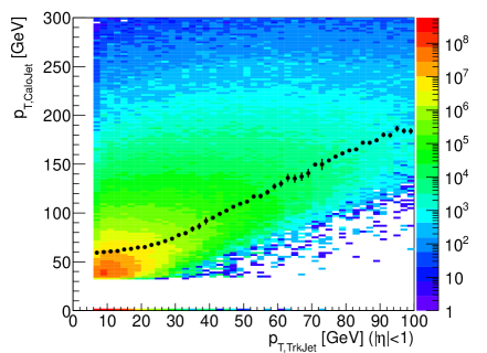
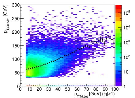
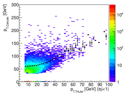
The centrality dependence of this energy scale was assessed directly by constructing ratios of distributions in central and peripheral collisions. Figure 5.6 compares this ratio as computed in data and MC. The ratios are roughly constant for track jets with GeV, away from the minimum calorimeter jet threshold, and each distribution is fit to a constant in this region. The values and errors of these fit parameters are shown in Fig. 5.7 for different centrality bins. The differences in the fit constants are evaluated directly in Fig. 5.8. The comparison indicates that the centrality dependence of the calorimetric response differs by no more than 2% between data and MC.
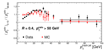
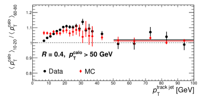
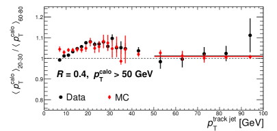
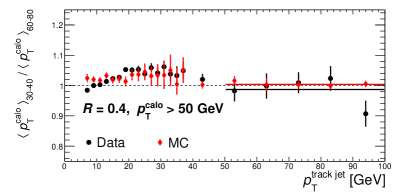
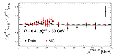
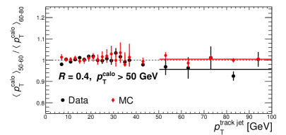
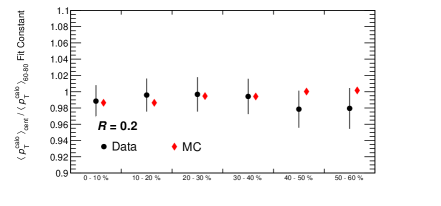
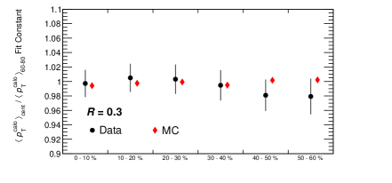
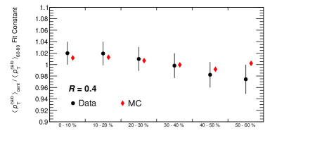
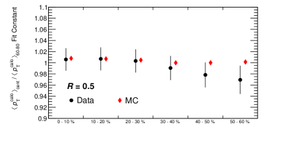

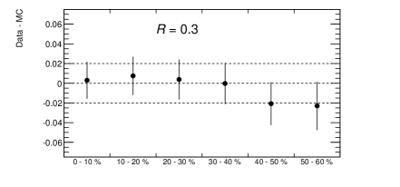
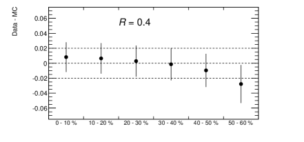
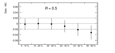
The jet energy scale calibration is sensitive to the particle composition and fragmentation of the jet. In particular it was found in events that the response was lower for broader jets [216]. One concern is that quenching effects could result in broader jets introducing a centrality dependence to the JES: a lower response in central collisions relative to peripheral. However, such an effect is not consistent with the results of the in-situ study as there is no evidence for the to be systematically below one.
5.3.2 Jet Energy Resolution
5.3.2.1 Fluctuations
To evaluate the accuracy of HIJING in describing the underlying event fluctuations seen in the data, the per-event standard deviation of the summed for all groups of towers has been evaluated. The numbers and were chosen so that the area of the group of towers had approximately the same nominal area as jets reconstructed with a given distance parameter , and values are given in Table 5.2. A complete systematic study is presented Ref. [218]; examples of that study are shown here. Figure 5.9 shows the event-averaged standard deviation as a function of the in the event for groups of towers, which have approximately the same area as jets. The same quantity is shown in both data and MC, with the MC scaled up by 12.6% to match the energy scale of the measured distribution. This procedure is equivalent to matching data to MC using fractions of the minimum-bias cross-section. The re-scaled MC results in Fig. 5.9 agree reasonably well with the results from the data over the entire range.
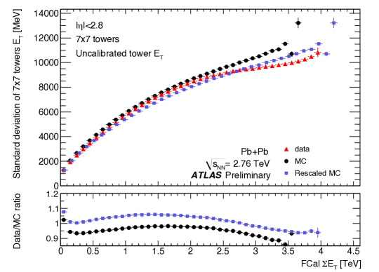
Based on this data-driven test of the MC, it can be concluded that the HIJING+GEANT simulations of underlying event fluctuations can differ from the data by at most 10%.
0.2 0.3 0.4 0.5
5.3.2.2 Jet Energy Resolution Validation
The knowledge of the size of the underlying event fluctuations can be used to validate the internal consistency of the jet energy resolution (JER) estimates. The jet energy resolution can be expressed in the following form
| (5.1) |
referred to as the stochastic, noise and constant terms respectively. The stochastic term represents fluctuations in the calorimeter shower sampling while the constant term relates to effects with such as dead regions. For the intrinsic energy resolution , the noise does not depend on the energy of incident particles and scales as for the relative energy resolution . The constant that quantifies the size of this term is the standard deviation of the noise energy and was evaluated in the fluctuation analysis described in Sec. 5.3.2.1. The JER was fit with the functional form of Eq. 5.1 with taken from the fluctuation analysis and and determined by the fit, and a sample of these fits is shown in Fig. 5.11. The values were adjusted slightly to account for the small differences in area between the rectangular tower groups and the nominally circular jet size, with area . The fit parameters and are found to be independent of centrality, confirming that the centrality dependence of the JER is related to the underlying event fluctuations in a quantifiable way. The noise term extracted from the fluctuation analysis is shown in the left panel of Fig. 5.10 as a function of the jet area for different centralities, along with a fit 111Although not directly relevant to jet performance, for all the centralities a fit value of was obtained. This hints at some structure in the fluctuations that should be investigated .
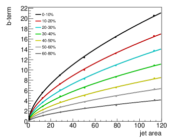
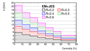
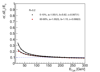
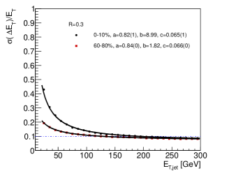
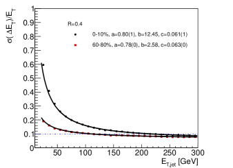
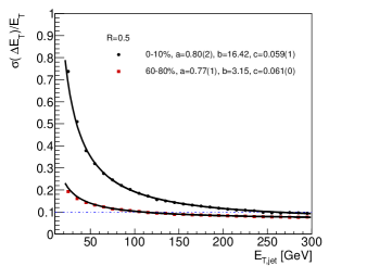
5.3.3 Data Overlay
To supplement the data-driven checks discussed in the preceding
sections, samples using MC jets from PYTHIA overlaid onto Pb+Pb data were also studied. These samples were generated by
combining minimum bias Pb+Pb events with PYTHIA dijet samples using
the pileup overlay framework [219] and performing reconstruction on the combined
signal. The PYTHIA events are produced in different J samples as
discussed in Section 4.2.
For each event the PYTHIA generation and subsequent GEANT simulation
is run with conditions matching data, including vertex position. The data events are taken from a dedicated MinBiasOverlay stream in
the 2011 running which uses a L1 ZDC coincidence trigger and records
the data without zero suppression.
The validation of these samples is not yet complete, and high statistics samples have not yet been produced, however aspects of the ongoing validation studies provide additional support of the data-driven checks presented in the preceding sections. The overlay samples used embedded J3 and J4 PYTHIA jets. These results are only meaningful over the jet range for which the J3 and J4 samples are the dominant contribution in the total cross section weighted sample ( GeV). The JES as a function of for jets is compared between 0-10% and 60-80% centrality bins in Fig. 5.12. This comparison indicates no dependence of the JES non-closure on centrality to the level of statistical precision allowed by the sample (). It is consistent with the estimates of the relative centrality-dependent JES non-closure derived in Section 4.4.1, and summarized in Fig. 4.16.
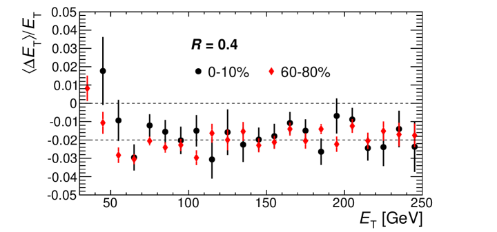
Comparisons were made of different performance variables between these overlay samples and the J3 and J4 embedded PYTHIA+HIJING samples in described in Section 4.2. A comparison of the JER between these two samples in central and peripheral collisions is shown in Fig. 5.13. Excellent agreement is found between the overlay and HIJING samples, consistent with the data/MC agreement found in the fluctuations analysis [218].
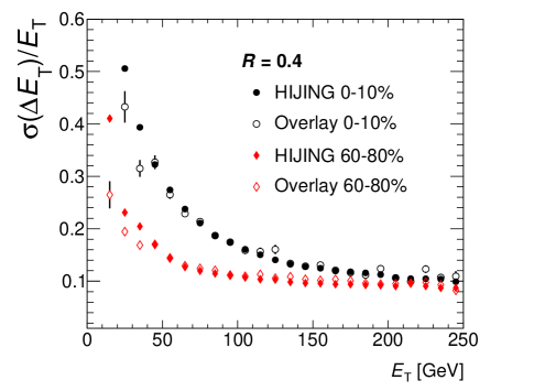
A similar comparison of the jet reconstruction efficiency is shown in Fig. 5.14. Above 50 GeV the peripheral efficiencies show good agreement, and there is a slightly greater efficiency ) in the HIJING sample in central collisions than in the overlay sample. As the J1 and J2 samples dominate at lower , the larger disagreement there is indicative of significant differences between the data and MC.
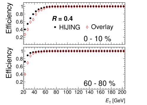
5.3.4 Jet Kinematics
As an evaluation of the jet in terms of and is sometimes preferred to and . For high- jets, it is expected that and will be very similar as will and . This was verified directly in data. The two-dimensional correlations in and in different centrality bins were computed in fine bins and are highly diagonal. The means of these distributions, vs and vs , are compared in central and peripheral collisions for jets in Fig. 5.15. No significant deviation from the behavior and is observed.
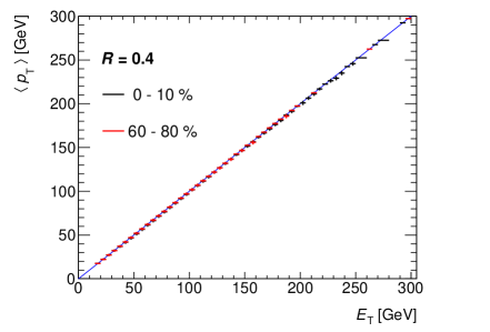
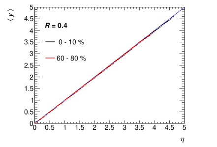
5.4 Unfolding
5.4.1 Observables
The goal of this measurement is to study jet quenching by examining the centrality dependence of the single inclusive jet spectrum. Collisions with different centralities have different degrees of geometric overlap between the colliding nuclei. This geometric effect translates into different per collision effective nucleon luminosities. Thus comparisons between different centrality bins should be scaled by , the effective number of colliding nucleon pairs in a given centrality bin, to remove the geometric enhancement. The “central to peripheral” ratio, , is defined as
| (5.2) |
The common phase space factors cancel, so the relevant quantity to extract from the data is the per event yield in bin ,
| (5.3) |
in each centrality bin. The 60-80% centrality bin is used as the peripheral bin in all and the notation is used to describe overall geometric enhancement as determined by the Glauber Model.
Jets from the 2010 Pb+Pb data set were reconstructed using the anti- algorithm with using the procedure described in Section 4.1 over the rapidity interval . All jets failing the fake rejection criteria described in Sec. 4.3.3 are excluded from the analysis. These spectra are shown in Figs. 5.16 and 5.17.
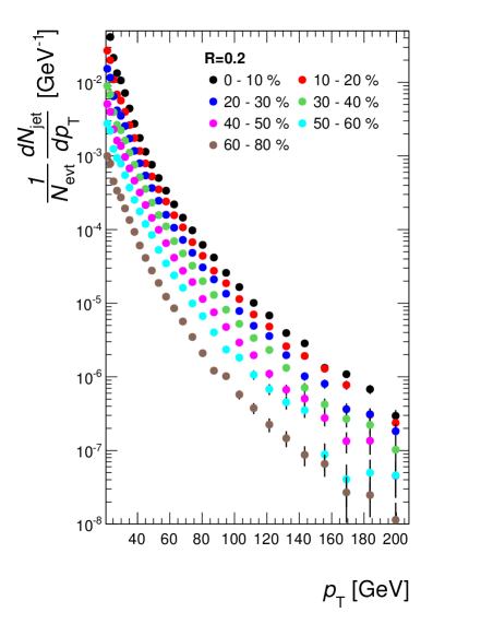
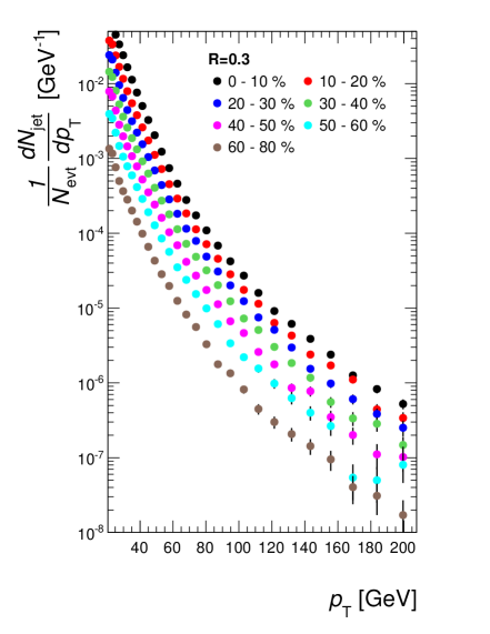
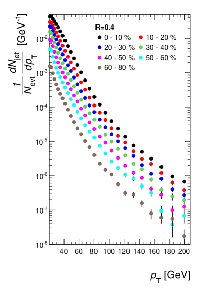
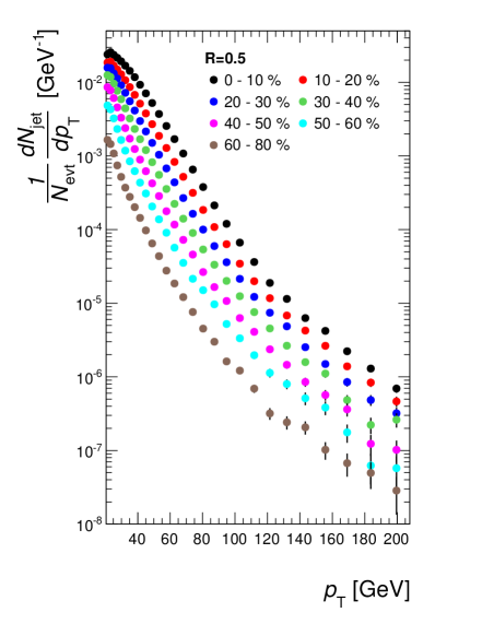
This measurement is a sampling of the per event jet multiplicity distribution in a given bin, which is given by the random variable and is sampled times. The measured per event yield is the mean of this variable,
| (5.4) |
A single event can produce multiple jets; this introduces a statistical correlation between bins and a full covariance matrix is required to describe the statistical uncertainty of the measurement described by
| (5.5) |
where the quantity
| (5.6) |
must also be recorded on a per event basis in addition to . The measured covariances are shown in Figs. 5.18 and 5.19, as the variance-normalized correlation
| (5.7) |
The matrix is strongly diagonal, indicating a weak correlation between different bins. However, the unfolding procedure will correct for bin migration and will introduce additional correlations between bins, resulting in a non-trivial covariance matrix.
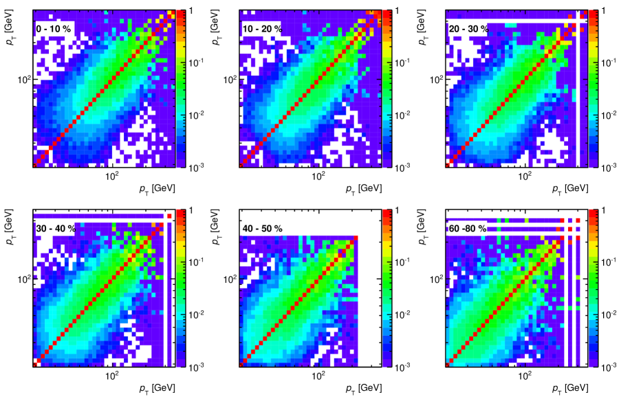
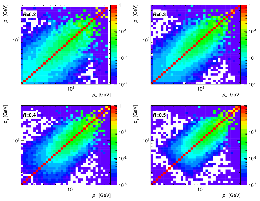
5.4.2 Method
The Monte Carlo is used to correct the raw spectrum for the finite jet energy resolution introduced by underlying event fluctuations and detector effects. For each truth jet, the nearest matching reconstructed jet with is found and the pair is recorded to build the response matrix . Then the input truth, , and output reconstructed, , distributions are related via a linear transformation
| (5.8) |
where is the full truth spectrum, including truth jets that had no matching reconstructed jet. If the Monte Carlo accurately describes the underlying event and detector response, a similar bin migration is assumed to apply to the measured spectrum, as well:
| (5.9) |
is the desired spectrum corrected for bin migration. The goal of an unfolding procedure is to invert this equation in a controlled fashion and obtain the true spectrum. The full inverse of the response matrix may possess properties introducing undesired features on the data, in particular the inversion may amplify statistical fluctuations. Additionally, the system of equations is over-determined and modifications to the linear system, motivated by the specific application, must be applied to have a well-determined solution. This study addresses these problems by using a singular value decomposition (SVD) based approach to regularize the unfolding as presented in Ref. [220]. The implementation of the SVD method in the RooUnfold software package [221] was used to perform the unfolding 222RooUnfold-1.1.1 was used with minor additions to allow for checks with continuous values of the regularization parameter..
The first modification to Eq. 5.9 is to recast the system in terms of a linear least squares problem, where each equation in the system is inversely weighted by the uncertainty in the measured spectrum ,
| (5.10) |
Thus equations with larger statistical uncertainty have less significance in the solution. In this framework the response matrix, , is expressed in terms of its SVD
| (5.11) |
where is a diagonal matrix containing the singular values,, and and are matrices composed of left and right singular vectors which each form orthonormal bases. For small singular values, can become large and statistical fluctuations in the data become magnified resulting in distortions in the unfolded distribution. To address this effect, the singular values are regularized by imposing smoothness requirements on the unfolded spectrum by expanding Eq. 5.10 to include the simultaneous minimization of the curvature of the spectrum,
| (5.12) |
where , is the second derivative of expressed in terms of finite differences and is a regularization parameter. The behavior for arbitrary is obtained by rewriting Eq. 5.9 as
| (5.13) |
and decomposing as in Eq. 5.11. The form of used in [220] and [221] assumes is filled using bins of fixed width. In this analysis, variable bins are used so that is constant, and thus is a finite difference approximation of . This measure of curvature is more appropriate given the steeply falling nature of the jet spectrum.
The behavior of the system under statistical fluctuations can be understood by analyzing the behavior of the data expressed in the basis supplied by the SVD
| (5.14) |
The are normalized by the error and statistical fluctuations are of order unity. The values of for which are the statistically significant equations in the linear system, and the number of such equations is the rank of the system . The remaining singular values correspond to statistically irrelevant equations and are regularized via
| (5.15) |
The final modification is to express the solution as a set of weights relative to another distribution ,
| (5.16) |
absorb the into the response, , solve for the weights
| (5.17) |
and multiply back by to obtain .
For well-determined systems, these operations have no effect on the solution. However when the system is overdetermined this is no longer true, and must be chosen carefully. In Ref. [220] it is argued that the truth spectrum, , used to generate is the proper choice of .
In this study it was found that the turn on of the efficiency, which results from a combination of reconstruction efficiency and fake rejection, introduced additional curvature and thus larger values of at low . This has the potential to propagate instabilities in the unfolding at low where the corrections are the least well known, throughout the entire spectrum, including regions where no efficiency corrections are required. Therefore the efficiency correction was removed from the unfolding problem by constructing to not include inefficiency. Then the unfolded spectrum is divided by to correct for efficiency in the final step after the unfolding is complete. To construct the MC truth spectrum was re-weighted by a smooth power-law to remove any statistical fluctuations in the MC then multiplied by the efficiency,
| (5.18) |
5.4.3 Response Determination
The SVD method relies on the curvature constraint to minimize the effects of statistical fluctuations on unfolding. This means that any non-smoothness in the response matrix or due to statistical fluctuations in the Monte Carlo sampling will distort the unfolding. To address this issue, the response matrices obtained from the Monte Carlo study were subjected to a series of smoothing procedures before begin used in the unfolding.
For each J sample, a two-dimensional histogram, , was populated from the of each truth-reconstructed matched jet pair. The distribution, without requiring a reconstructed jet match, is was also recorded in a histogram . The and from the different J samples are then combined using the cross section weighting discussed in Section 4.2. The response matrix was then constructed from these two distributions
| (5.19) |
which satisfies Eq. 5.8 if there is no inefficiency. One-dimensional distributions, obtained by projecting in fixed slices, are typically Gaussian-like with integrals equal to the total efficiency in that bin. The tails of these distributions are often produced by cases where a single truth jet is reconstructed as a pair of split jets and vice versa and can display behavior that is qualitatively different than the rest of the distribution. While this represents a small effect on the bin migration, the changes in shape may cause problems with the additional smoothness constraints in the SVD method. Thus contributions to each slice less than % were removed and the rest of the distribution rescaled to keep the integral the same. The one dimensional slice of this distribution after smoothing for jets in the 0-10% centrality bin are shown in Fig. 5.20. Checks were performed to test the sensitivity to this cutoff that showed no significant change in the final results with this cut removed.
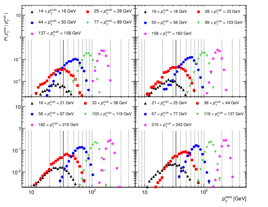
The binning used for the spectra and response matrices cover the range . The bin boundaries for the bin, and , were chosen such that is independent of and fixed by the number of bins. The unfolding was performed on an interval, , of this range chosen based on requirements of the unfolding procedure. To allow proper bin migration in both directions the range of values allowed for the unfolded spectrum must exceed the range of the reconstructed values on both sides ( and ). The unfolded result should then only be used over the reconstructed range, possibly excluding the most extremal bins on either edge of this range due to bias. The linear system is under-determined unless there are at least as many reconstructed bins as truth (unfolded) bins on their respective ranges. A bin selection satisfying these requirements is summarized in Table 5.3.
Bin low Bin high [GeV] [GeV] Truth 35 1.15 5 27 12 320 Reco 60 1.09 20 44 34 270
5.4.4 Statistical Uncertainties
The measured covariance is used to generate statistical uncertainties in the unfolded spectrum by using a pseudo-experiment technique. A pseudo-experiment consists constructing a new input spectrum, which is then unfolded. The procedure uses the measured covariance of the data to generate a new spectrum consistent with correlated Poisson fluctuations of the measured spectrum. 1000 pseduo-experiments are performed, and the statistical covariance of the distribution over all such pseudo-experiments is a measure of the effect of the statistical uncertainty of the measured spectrum on the unfolded result.
The effect of statistical fluctuations in the MC used to obtain the response matrix is computed in a similar fashion. In this case each pseudo-experiment uses a different response matrix, which is a possible statistical fluctuation of the input response matrix. These fluctuations are generated by using the error on the matrix element to generate a new value of the matrix element consistent with a Poisson fluctuation of the original. The total statistical covariance is taken to be the sum of the covariance matrices obtained from these two procedures, which is equivalent to summing the uncertainties in quadrature.
The unfolding method systematically associates features of the unfolded spectrum with statistical fluctuations and damps their contributions to the result through regularization. It is expected that increases in the regularization parameter may artificially reduce the sensitivity of the unfolding procedure to statistical fluctuations in the input spectrum. This effect is shown in Fig. 5.21, where the statistical errors on the have been evaluated using the pseudo-experiment technique for values of from 4 to 10, with the statistical errors on the measured spectrum before unfolding shown for reference. The maximal value of was chosen to be 10, which is approximately half the number of bins in the reconstructed sample with finite counts. This corresponds to the Nyquist frequency of the system: the highest value that can be included without introducing aliasing effects in the signal decomposition and reconstruction.
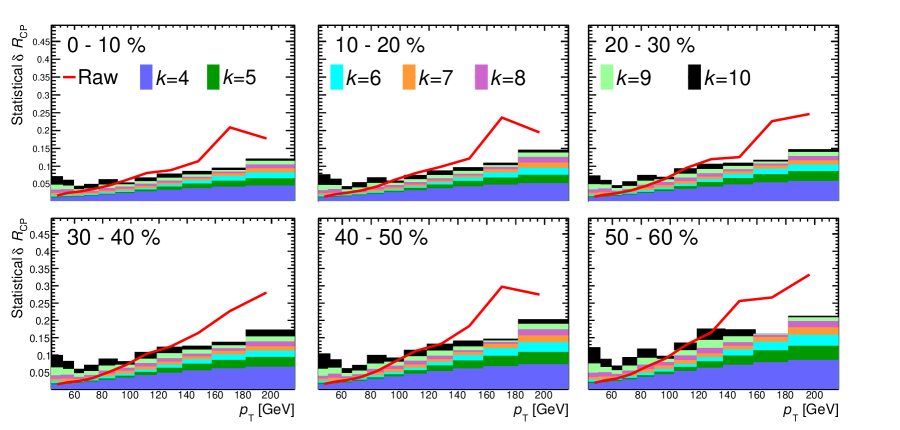
5.4.5 Distributions and Refolding
The choice of the regularization parameter is driven by the distribution of values as defined in Eq. 5.14. The coefficient is the projection of the data (error normalized) onto the direction associated with the th largest singular value. For values of , the corresponding equation in the now diagonal linear system is statistically well determined. Values of of order unity are consistent with statistical fluctuations in the data that select out a particular singular value. The contributions from these equations, which become large when the matrix is inverted, must be regulated. From these considerations, the value of is chosen where the distribution transitions from statistically relevant equations to equations consistent with statistical fluctuations. The distributions for the jets are shown in Fig. 5.22. was chosen for all centrality bins and values.
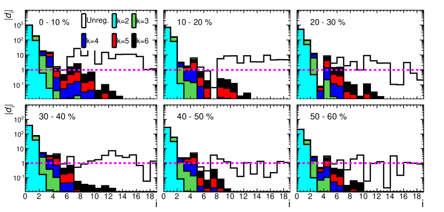
Choosing to be too small (or equivalently choosing too large) will over-regularize the result by removing relevant information from the response matrix. Thus the choice of must be made in conjunction with a refolding test, where the unfolded spectrum is multiplied by the full, unregulated response matrix and compared to the input spectrum. To make this comparison more rigorous both in justifying the choice of and providing a mechanism for analyzing the systematics, Eq. 5.15 was extended to consider continuous values. The refolded spectrum is compared to the original measured spectrum, and the degree of closure of the operations is quantified by a ,
| (5.20) |
where is the measured covariance of the data. Since is the solution to the unfolding problem constructed from , the fluctuations on and the refolded spectrum are not statistically independent. This means that this is not a sum of squares of independent variables with unit normal distribution, and does not follow a probability distribution. Despite this limitation, this variable, especially its behavior as a function of , is still useful in describing the refolding closure so long as it is not misinterpreted.
The distribution of the refolded as a function of is shown in Fig. 5.23. The growth in at large in the neighborhood of the smallest values shows that such regularizations remove enough information to prevent closure in the refolding. Small values of maintain a faithful refolding procedure, with low , at the expense of amplifying statistical fluctuations in the unfolded spectrum.
Under-regularization will allow statistical fluctuations to become amplified in the unfolding. Once an appropriate choice of is made, the curvature of the weights distribution can be used to quantify the extent to which this effect occurs. There are two sources of curvature in the weight distribution: statistical fluctuations and differences between the unfolded spectrum and . The optimal regularization point occurs when the statistical fluctuations have been suppressed, but differences between and the unfolded spectrum are not smoothed away. As the sources of curvature are changing near this value of it is expected that the curvature distribution will change shape in this region. The curvature as a function of is shown overlaid with the distributions in Fig. 5.23. Regions of flatness in the overlap in with the qualitative changes in the curvature distribution.
The procedure for extracting statistical uncertainties on the unfolded spectrum is discussed in Section 5.4.4. This addresses the question of how sensitive the unfolded spectrum is to statistical fluctuations on the measured spectrum for a given regularization procedure (i.e. choice of or ). It is possible that were a different statistical fluctuation of the data observed, a different regularization procedure could have been chosen, which is more sensitive to statistical fluctuations. This would occur if different fluctuations had different and curvature distributions as functions of . To check the stability of these distributions, the pseudo-experiment method was again used where these two distributions were generated for many possible fluctuations of the data. The stability of the two distributions under statistical fluctuations indicates that choice of regularization would not change under statistical fluctuations, and further justifies the procedure described in Section 5.4.4 as a full measure of the statistical uncertainty.
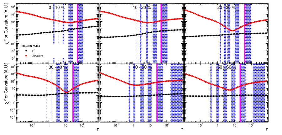
5.5 Systematic Uncertainties
Systematic uncertainty on the final, unfolded result is estimated both from ingredients from the MC into the unfolding and the unfolding procedure itself. For some sources, the uncertainties in are point-wise correlated, e.g. in vs. changes in the JER cause all points in the curve to move up/down together. Such systematics are indicated by continuous lines drawn around the values of the . Which systematics show point-wise correlations depend which variable the is being plotted against and are summarized in Table 5.4. As the is a ratio between two different centrality bins, errors that are correlated in centrality are taken from the variation of the due to that systematic. Errors on the due to sources that are uncorrelated in centrality are taken as independent errors on the central and peripheral spectra and combined in quadrature. Errors that show no point-wise correlation are shown by shaded boxes and indicate the maximal variation of the points independent of one another due to such systematics. The relative error of each individual contribution to the systematic error on vs is shown in Figs. 5.24 and 5.25.
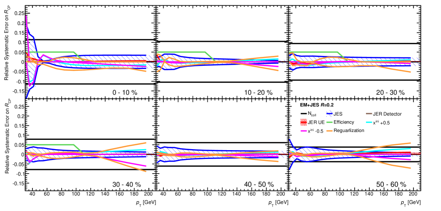
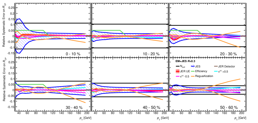
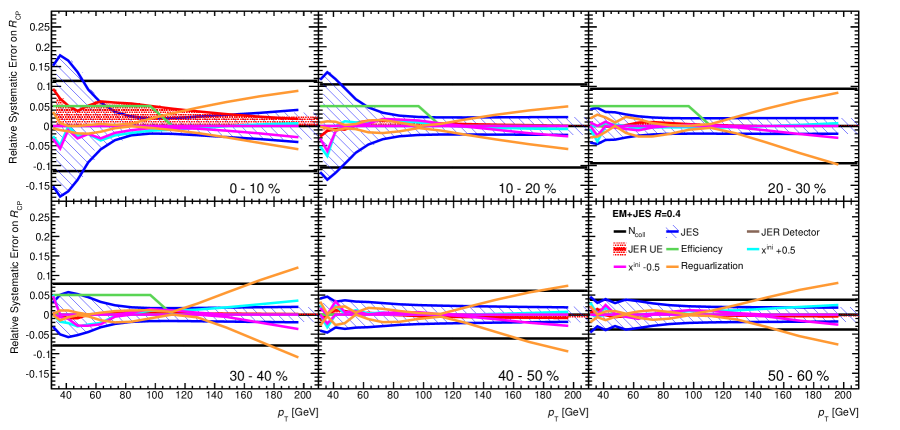
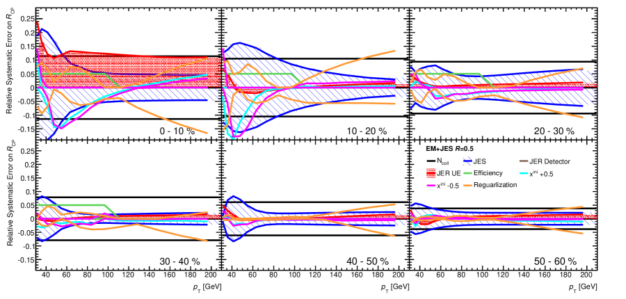
Systematic Centrality Regularization Efficiency JES JER
5.5.1 Regularization
The systematic uncertainties associated with the unfolding procedure were estimated by considering the sensitivity of the procedure to the regularization parameter. The unfolding was performed with a different value of and the variation in the unfolded spectra were taken as systematic errors. The errors on the central and peripheral spectra were then combined to determine an error on the . Independent systematics were generated for both increased and decreased regularization by unfolding with and .
An alternative estimate of the systematic uncertainty associated with under-regularization was also tested and gave similar results as regularizing with the . This evaluation was motivated by linear least squares problems where the systematics are commonly estimated by considering variation of the by 1 about the minimum value
| (5.21) |
The unfolding problem is not a strict minimization of the as monotonically increases with . Thus for the purposes of estimating the effect of increasing , the system is effectively at a minimum and the above estimate was used to determine a value. The spectra were unfolded with this and the variation in the spectra were used as above to generate a systematic on the .
5.5.2 and Efficiency
One advantage of the SVD procedure is that the unfolded result is less sensitive to the choice of than the truth spectrum used in a bin-by-bin unfolding procedure. To test this sensitivity the power in Eq. 5.18 was varied .
In peripheral collisions the fake jet rate is expected to be vanishingly small above GeV. The fraction of jets remaining after fake rejection as a function of in peripheral data is consistent with the same quantity in all centralities in the MC as shown in Fig. 4.8. There is a small deviation at the highest where the MC does not fully saturate. However, this disagreement is present in all centrality bins and divides out in the . No systematic error was taken from this aspect of the efficiency.
The uncertainty on the jet reconstruction efficiency prior to any fake rejection was estimated by comparing efficiencies in the HIJING sample and the overlay. The uncertainty in the ratio of central to peripheral efficiencies was taken conservatively to be for GeV for all centralities and values.
5.5.3 Energy Scale
Systematic uncertainties in the jet energy scale can arise both from disagreement between the MC, where the numerical inversion constants are derived, and data, as well as systematic shifts in the energy scale between different centralities associated with the underlying event subtraction. The former source only affects the absolute jet energy scale uncertainty which divides out in the . This is true to the extent to which the changes in absolute scale do not distort the unfolding differently in different centralities.
Relative changes in the energy scale between central and peripheral collisions are estimated by combining two studies. The difference in closure in the MC JES analysis, as presented in Sec. 4.4 provides sensitivity to the effect of the background subtraction on the JES. Additionally, the in-situ JES validation comparing the track-calorimeter jet energy scales in Sec. 5.3.1.2 provides further constraints as it is sensitive to differences in jet fragmentation between the two centralities.
Using these studies as input, systematic uncertainties were estimated on the energy scale for each centrality relative to the peripheral and are shown in Table 5.5. The MC samples were processed adding an additional shift, , to the of each reconstructed jet when filling out the response matrices. A constant shift was applied above 70 GeV. Below the shift value was a linear function of , increasing to twice the high- value at 40 GeV,
| (5.22) |
where is the value given in Table 5.5. The data was unfolded using the new response matrices resulting in a modified spectrum used to compute a new . Variations from this from the original in each bin were taken as symmetric errors due to this systematic.
0 - 10 % 10 - 20 % 20 - 30 % 30 - 40 % 40 - 50 % 50 - 60 % 0.2 0.5 % 0.5 % 0.5 % 0.5 % 0.5 % 0.5 % 0.3 1.0 % 0.5 % 0.5 % 0.5 % 0.5 % 0.5 % 0.4 1.5 % 1.0 % 0.5 % 0.5 % 0.5 % 0.5 % 0.5 2.5 % 1.5 % 1.0 % 0.5 % 0.5 % 0.5 %
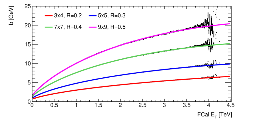
5.5.4 Energy Resolution
To account for systematic uncertainties coming from disagreement
between the jet energy resolution in data and MC, the unfolding
procedure was repeated with a modified response matrix. This response
matrix was generated by repeating the MC study but with modifications
to the for each matched truth-reconstructed jet
pair. A “detector” systematic was constructed to account for
uncertainty between the data and MC without considering the effects of
the underlying event. This procedure follows the recommendation for
JER uncertainty in 2010 jet analyses in . The
JetEnergyResolutionProvider
tool [222] was used to retrieve the fractional
resolution, as a function of jet and [223]. The jet
was then smeared by
| (5.23) |
where is the unit normal distribution.
A separate systematic uncertainty considering the effect of disagreement of underlying event fluctuations in the data and MC was also determined. As discussed in Section 5.3.2.2, MC is internally consistent between the tower RMS distributions and the JER as a function of as expressed in Eq. 5.1. The term is sensitive to fluctuations in the underlying event, while the and terms are independent of centrality. This is shown in Fig. 5.11, where fits of the JER with this form only differ significantly in the value of the parameter. Additionally, the underlying event fluctuations, as measured by the RMS of the distribution of tower groups, is consistent with the value obtained from the fit of the JER for jets with the same area.
The MC fluctuations, which give as a function of FCal are fit with the functional form
| (5.24) |
which is shown in Fig. 5.26, and the values of the fit parameters , , and for the different values are presented in Table 5.6 along with maximal estimates of the MC/data deviation of these distributions given by the quantity .
0.2 2. 5 94. 4 0. 622 0. 0083 181. 0 0.3 2. 5 81. 9 0. 641 0. 0133 89. 3 0.4 5. 0 75. 1 0. 680 0. 0168 50. 5 0.5 7. 5 75. 4 0. 712 0. 0176 38. 8
As in the detector systematic, a new response matrix was constructed. The was rescaled by an amount
| (5.25) |
is determined from the and is chosen to account for differences in the fluctuations between data and MC based on the values of shown Table 5.6. In most central 10% of collisions the tower distributions in the MC are broader than the data, so the effect of the fluctuations was symmetrically reduced by using . This systematic was applied as a one-sided error to the most central bin. Any other differences in the RMS results from the data having larger downward fluctuations, but smaller upward fluctuations. To account for this effect the was chosen for and for . This was applied as an asymmetric error to all but the most central bin. In no region of centrality does the data have larger upward fluctuations than the MC.
5.5.5 Uncertainties
The uncertainties in the values obtained from the centrality analysis are shown in Table 5.1. The errors reported for all centrality bins are partially correlated because individual variations in the sensitive parameters in the Glauber calculation cause all values to increase or decrease together. To evaluate the systematic uncertainties in the ratios of between two centrality bins, , that appear in the expression for we have directly evaluated how this ratio varies according to variations of the sensitive parameters in the Glauber Monte Carlo. We obtain from this study separate estimates for the uncertainty in the ratios; the results are provided in Table 5.1.
5.5.6 Consistency Checks
In addition to the systematic variations discussed previously, cross checks were performed by varying aspects of the analysis. These checks serve to test self-consistency of the procedure, not to quantify sensitivities to quantities expected to be uncertain. One such example is the fake rejection scheme, where it is natural to consider whether the default scheme imposes a fragmentation bias on the jets included in the spectrum and the . An alternative fake rejection scheme was assessed where the track jet matching requirement was replaced by a single track match within of the jet axis, where the track is subject to the following selection criteria:
-
•
GeV
-
•
mm
-
•
-
•
-
•
These requirements are significantly looser than those required on the tracks input into the track jet reconstruction. Although these looser matching criteria may lead to increased sensitivity to fake jets at low , as long as the fake rate is not dramatically enhanced, the lower threshold (4 GeV vs 7 GeV for track jets), should address any concerns regarding a fragmentation bias. An identical analysis was performed using measured spectra and response matrices generated from this alternate scheme. The ratio of the values to those from the default scheme is shown in Fig. 5.27, with the statistical errors taken from errors generated on the nominal through the pseudo-experiment method. The values show good agreement to the level of a few percent. The residual difference, an enhancement at low that decreases with centrality, is consistent with the expected slight increase in fakes.
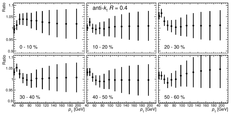
The GCW calibration scheme has a reduced sensitivity to jet width and flavor content relative to the EM+JES [216]. A comparison between these two calibration schemes was performed and the ratio of the obtained from the two schemes prior to unfolding is shown for jets in Fig. 5.28. The distribution shows good agreement, indicating that the calorimeter response is not significantly altered for quenched jets.
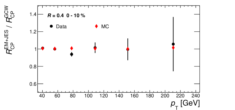
Consistency checks were performed to investigate any biases introduced by the unfolding procedure or the choice of binning and range. The reconstructed spectrum from the MC sample was treated like the data and unfolded. The unfolded spectrum was then compared directly to the MC truth, and the ratio is taken to quantify the closure of the unfolding procedure. Since the final physics result is the , the bias on this quantity was also investigated. For each centrality bin the unfolded spectrum was divided by the unfolded spectrum in the 60-80% centrality bin to form an (with no factor). The analogous quantity was constructed from the MC truth and the ratio of the ’s was taken. Finally, a refolding test was preformed. When the unfolding was performed on the data, only this last check was possible. Any relationship between the unfolding non-closure in MC truth and MC refolding provides a context for interpreting the refolding in data as a potential bias on the unfolded data result.
The results of this test are shown in Fig. 5.29, regularized with , for the jets. The MC truth non-closure shows some structure at the 5% level which is common to all centrality bins and values (not shown). This structure is associated with the finite regularization parameter, and the effects can be removed by increasing . Since the MC sample has much higher statistics than the data, the optimal value of is likely to be much higher in the MC than in the data, and can be increased without introducing strong effects from statistical fluctuations in the reconstructed spectrum. To facilitate the comparison with data, the value of was chosen to be near the values appropriate for the data, and thus the MC unfolded spectrum is slightly over-regularized. Nevertheless the comparison shows good closure and insignificant systematic bias in the procedure. The shows even less bias as some of the structure is common to all centrality bins. The refolded reconstructed spectrum shows similar structure, suggesting that this check will be sensitive to residual bias in the data.
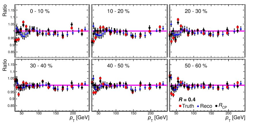
Chapter 6 Results
6.1 Jet Spectra and
6.1.1 Unfolded Spectra
The unfolded spectra are shown in Figs. 6.1 and 6.2 including the effect of the efficiency correction. The ratios of these spectra to the raw distribution as well as the refolding closure test are shown in Figs. 6.3 and 6.4. The unfolding procedure alters the measured statistical correlations between bins resulting in large off-diagonal covariances. These covariances were obtained using the method described in Section 5.4.4 and are shown in Figs. 6.5 and 6.6.
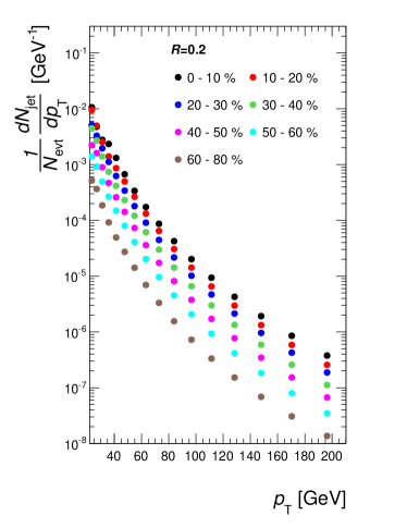
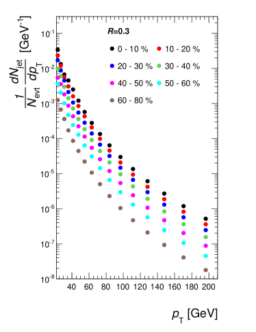
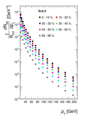
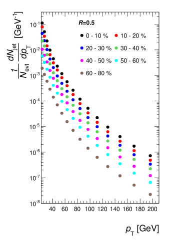
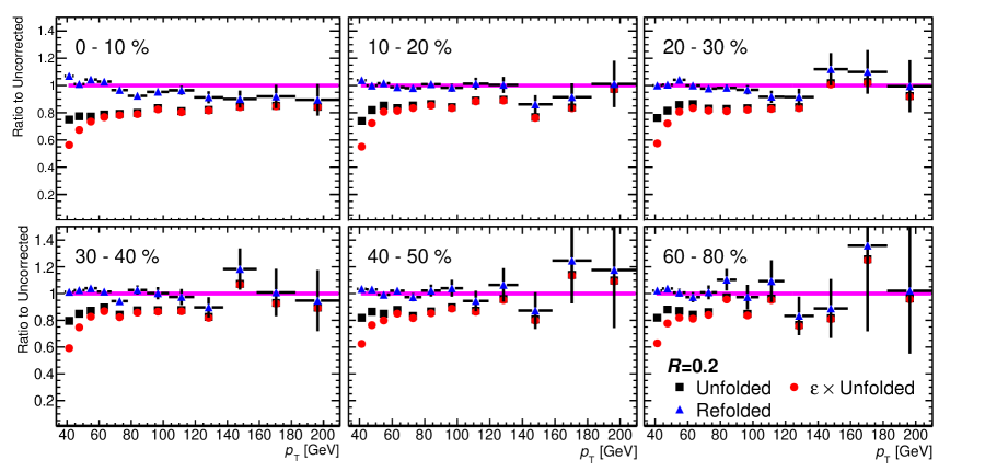
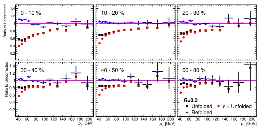
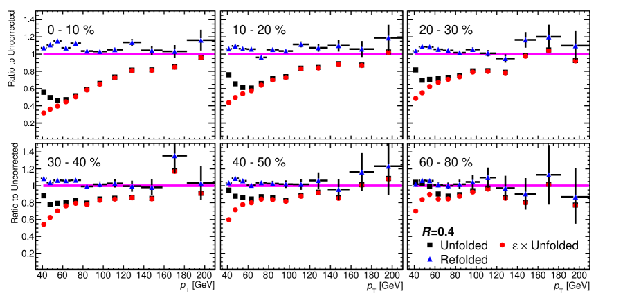
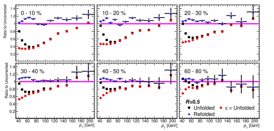
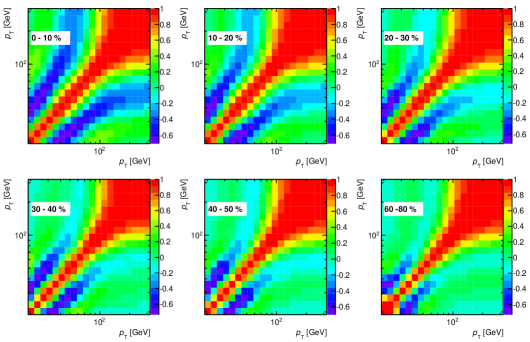
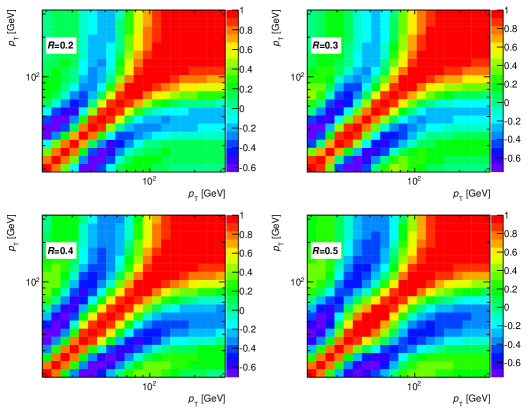
6.1.2
The jet as a function of are shown in Figs. 6.7 - 6.10 with the black bands and shaded boxes representing the correlated and uncorrelated errors composed of the sources indicated in Table 5.4. A subset of the results for the and jets are presented in a slightly different fashion in Figs. 6.11 and 6.12. In these figures the -dependences of selected centrality bins is compared in different vertical panels. These results indicate that jets are suppressed in the most central collisions by approximately a factor of two relative to peripheral collisions. For all jet radii, the suppression shows at most a weak dependence on jet . The correlated systematic error bands indicate that there may be a slight increase in in the range GeV, although this is not present in all centralities and radii. For some bins, the shows a mild decrease with increasing at the highest values, this effect is also marginal within the systematic errors, and will be discussed further in Chapter 7.
The as a function of centrality, as expressed by the average number of participants in each centrality bin, is shown for different bins in jet in Figs. 6.13 - 6.16. Note that the composition to the two types of systematic errors changes when plotting vs centrality as opposed to vs . In general the dependence shows a weak dependence on jet . The dependence for the lowest bins, shows a linear drop in in the most peripheral collisions before flattening out. This dependence is slightly different than in the highest bins, where the dependence is more linear throughout the full range.
Finally the dependence of the is evaluated directly. This comparison is shown for the 0-10% centrality bin for different bins in Fig. 6.17. A comparison of this dependence for different centrality bins but at fixed , GeV, is shown in Fig. 6.18. These results indicate an at most weak reduction in the suppression with increasing jet radius. There is essentially no reduction in suppression in the 50-60% bin, where there is a slight increase in the with in the most central bin.
An alternative evaluation of the dependence of the on jet radius is provided in Fig. 6.19 which shows the ratio of values between and 0.5 jets and jets, , as a function of for the 0-10% centrality bin. When evaluating the ratio, there is significant cancellation between the assumed fully correlated systematic errors due to , JES, JER, and efficiency. The results in the figure indicate a significant dependence of the on jet radius for GeV in the most central collisions. For lower values, for both and differ from one beyond the statistical and systematic uncertainties. The maximal difference between the and jets occurs GeV, where exceeds 1.3. The central values for jets also differ from one, but that difference is not significant when the systematic errors are accounted for.
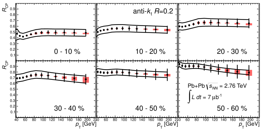
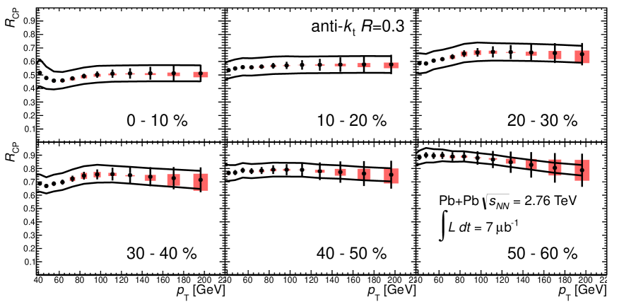
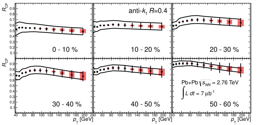
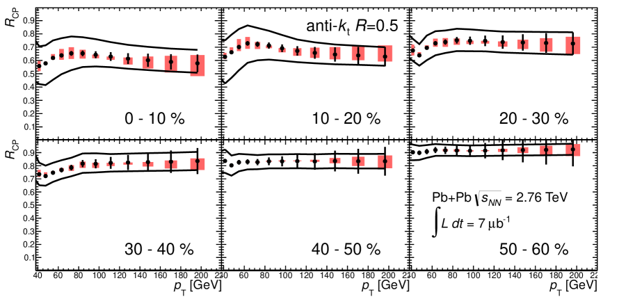
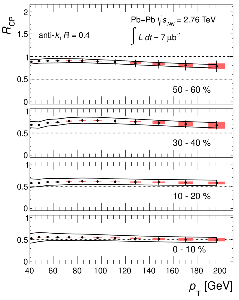
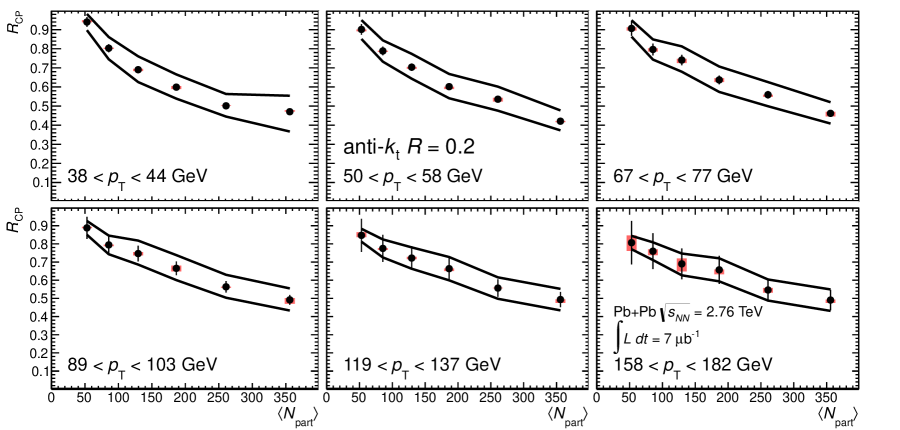
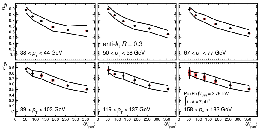
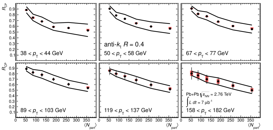
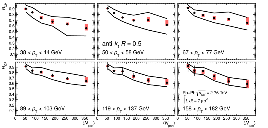
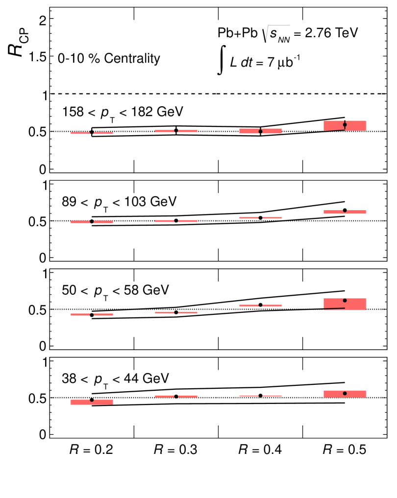
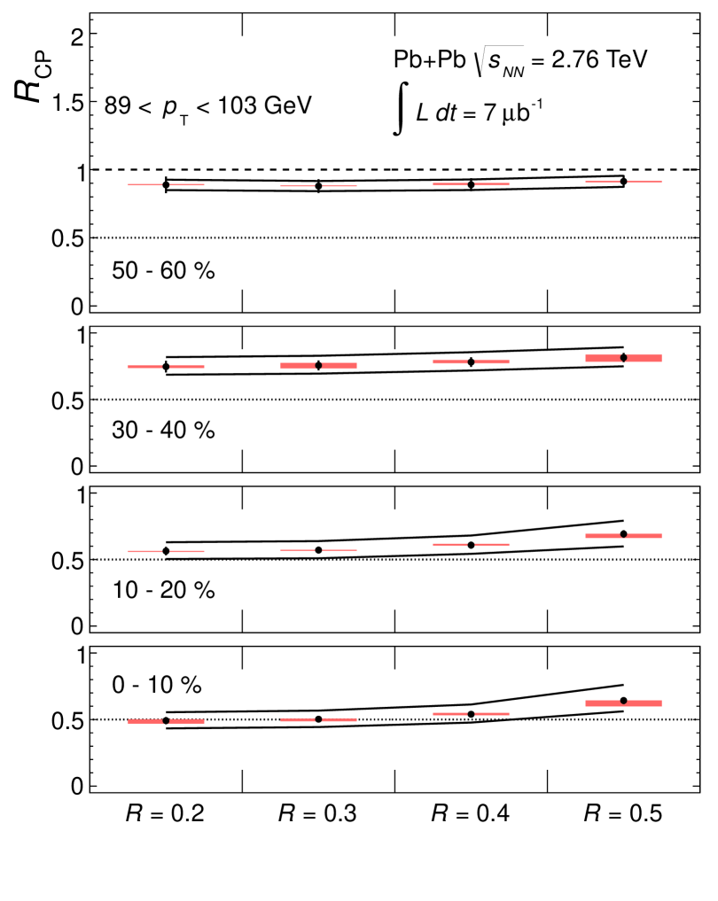
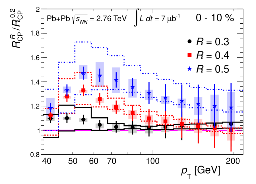
6.1.3 Energy Loss Estimate
If a simple model of energy loss is assumed, the -dependence of the can be isolated. Following the discussion in Ref. [224], an that is independent of can be the consequence of energy loss that is proportional to the jet’s original . The number of jets measured at a final after energy loss, , will be populated by jets that were produced with an original momentum of ,
| (6.1) |
If the unmodified (i.e. initial) jet spectrum is described by a power law which is independent of centrality,
| (6.2) |
The final measured spectrum is modified by the transformation from to :
| (6.3) |
If the energy loss is defined relative to peripheral collisions then the initial and measured spectra are equal,
| (6.4) |
In central collisions the measured spectrum is related to the initial by,
| (6.5) |
Therefore the and lost energy fraction, , are related by
| (6.6) |
The centrality and dependence of have been extracted from the measurements made here of for GeV, where the assumptions of power law spectrum and -independent are appropriate. The power, , was obtained from fitting the spectra in the 60-80% centrality bin, and the extracted fit constants and errors are shown in Table 6.1.
| 2 | 5.49 0.07 | 0.90 0.10 | 8.21e-04 5.87e-05 |
| 3 | 5.64 0.07 | 0.88 0.14 | 9.13e-04 4.92e-04 |
| 4 | 5.72 0.06 | 0.88 0.20 | 7.46e-04 4.38e-04 |
| 5 | 5.78 0.06 | 0.74 0.12 | 1.25e-03 7.81e-04 |
In each centrality bin the was fit to a constant, , by minimizing the function,
| (6.7) |
Here is the full covariance matrix of , which contains contributions from statistical correlations, uncorrelated systematic errors and correlated systematic errors. The statistical covariance was obtained in Chapter 6. For uncorrelated systematic errors, the covariance matrix was taken as diagonal , and for fully correlated errors the covariance matrix is . The solution to the minimization, is expressed analytically in terms of the full covariance as
| (6.8) |
An uncertainty on this quantity was determined by varying such that the per degree of freedom differed from its minimum value by one. This analysis was performed in each centrality bin for all values with the resulting evaluation of shown in Fig. 6.20.
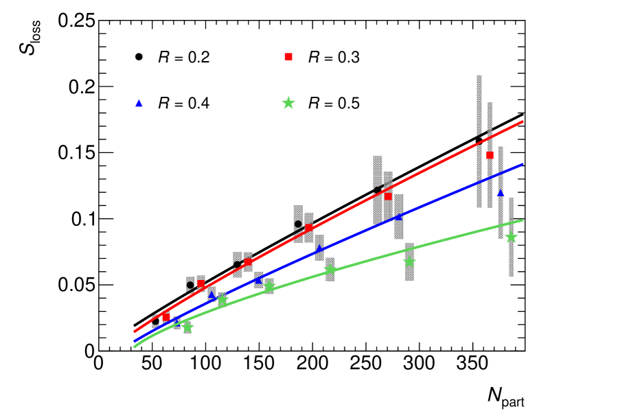
The grey boxes indicate the combined error due to uncertainties in both and with the horizontal size determined by the uncertainty on given in Table 5.1; the points have been artificially offset to facilitate comparison. The smaller radii show a nearly linear growth in with . However the rate of growth diminishes with increasing value indicating that some of the lost energy may be recovered with the larger jet definition. To provide a quantitative estimate of the dependence, the for each value was fit with the functional form,
| (6.9) |
with the fit values of and and their associated fit errors shown in Table 6.1 and the fit functions shown with the points on Fig. 6.20.
6.2 Dijet Asymmetry
The observation of a centrality-dependent dijet asymmetry was the first indication of jet quenching at the LHC and was reported by ATLAS in Ref. [1]. That publication was a snapshot of an ongoing, more extensive asymmetry analysis which is one of the main results of this thesis. The results presented here improve on the first published result by using the increased statistics of the full collision data set and benefiting from improvements in the jet reconstruction performance. These results were presented at Quark Matter 2011 [225, 226] and are presented more thoroughly in Ref. [227]. It should be noted that the jet reconstruction procedure has evolved between the completion of the asymmetry analysis and the analysis. In fact, these improvements were a significant technical undertaking designed to improve the performance and enhance the precision and reach of the measurement. The reconstruction procedure and performance as documented in previous chapters coincides with the analysis. While main features of the background subtraction (seed finding, flow correction and iteration step) were also present when the asymmetry analysis was performed, the details differ slightly (flow iteration step, cut on seeds). Those details and the performance of that version of the reconstruction are documented Ref. [227], and generally will be omitted here. One important distinction is the lack of jet energy scale calibration constants for jets at the time of the asymmetry analysis. An analysis of the asymmetry for jets was performed using the calibration constants. The result is a non-closure in the JES, which drops to at the lowest ’s. This effect, shown in Fig. 6.21 for the 0-10% and 60-80% centrality bins, is independent of centrality and largely cancels in the asymmetry. The jets do not suffer from this problem.
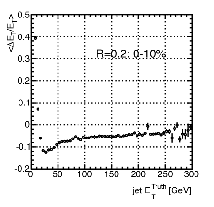
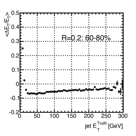
Following the procedures used in Ref. [1] the per-event dijet asymmetries are calculated according to
| (6.10) |
where is the transverse energy of the leading (highest ) jet in the event and is the transverse energy of the highest jet in the opposite hemisphere ( with the azimuthal angle difference between the jets). Both jets are required to satisfy the requirement. Events for which the second highest jet in the event fails the or requirements are not excluded, but rather the highest jet that does satisfy these criteria is used. All presented results have the requirement GeV; events for which the second jet (passing the above selections) fails this requirement are excluded from the analysis.
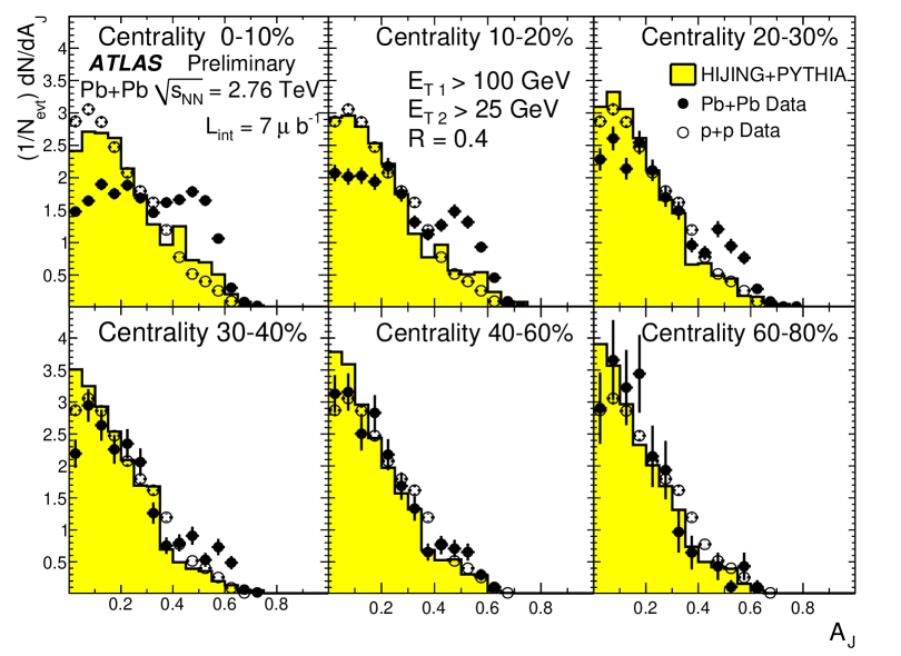
Figure 6.22 shows the asymmetry distribution for jets with GeV for six bins of collision centrality. Also shown for each centrality bin are results obtained from measurements at 7 TeV [228] and the asymmetry distributions obtained from the HIJING+PYTHIA MC samples for the corresponding centrality bin using the above described analysis procedures. The features observed in the original dijet asymmetry publication are seen in Fig. 6.22, namely good agreement between Pb+Pb data, data, and MC results in the more peripheral (40-60% and 60-80%) centrality bins and an increasingly strong modification of the asymmetry distributions for more central collisions. The MC distributions show modest broadening from peripheral to central collisions due to the increased underlying event fluctuations. However, the modifications seen in the data are much stronger than those seen in the MC for which the underlying event fluctuations are shown to be consistent with those in Pb+Pb data in Fig. 5.9.
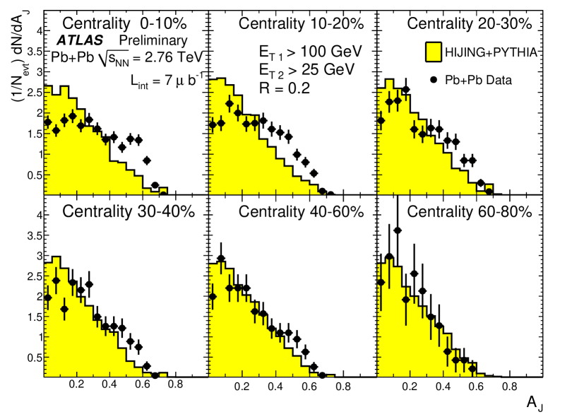
Figure 6.23 shows the measured asymmetry distributions for jets with GeV compared to results from MC simulations. An analysis of data with is not yet available. The asymmetry distributions show the same general features as seen in the results shown in Fig. 6.22. However, the asymmetry distributions generally extend to slightly larger values for jets than for jets. Another difference between the and results can be seen in the 40-60% centrality bin where a modification of the asymmetry distribution is seen for jets and not for jets.
One of the most important results presented in the original dijet asymmetry letter was the observation that the dijet distribution remains mostly unchanged in all centrality bins while the asymmetry distribution is strongly modified in central collisions. Figures 6.24 and 6.25 show updated results for the distributions for dijets with GeV using the same dijet selection procedure described above. Both linear and logarithmic vertical scales are shown. These figures confirm the original observation that the dijet distributions are unmodified with the caveat that a small combinatoric contribution is observed in the 0-10% and 10-20% centrality bins. Such a combinatoric contribution was also seen in the original measurement. The dijet distributions for jets with GeV are shown in Figs. 6.26 and 6.27 with linear and logarithmic vertical scales, respectively. The distributions show no modification and a much smaller combinatoric contribution.
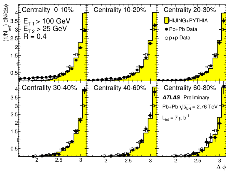
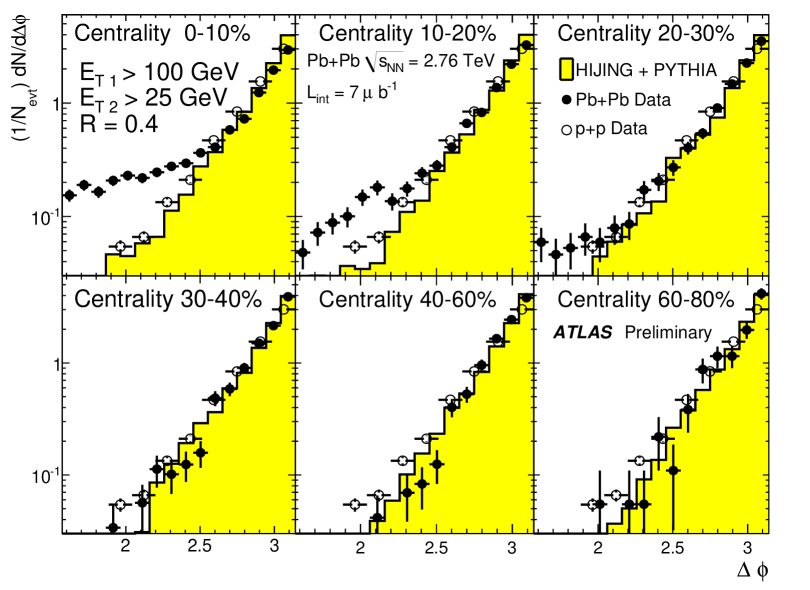
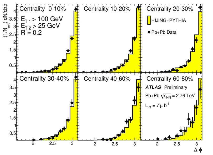
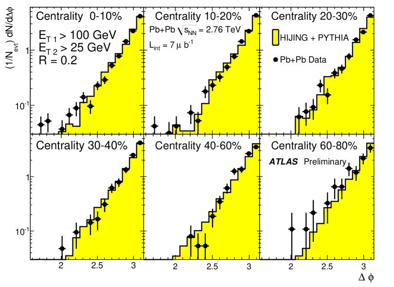
The evolution of the asymmetry with the threshold is shown in Figures 6.28 and 6.29, which contain distributions of dijet for three different centrality bins, 0-10% (top), 30-40% (middle), 60-80% (bottom), for three different ranges of energies (see figures) for the leading jet. The peaking at larger values of becomes more pronounced when is restricted to a lower range and that peaking becomes less pronounced as increases. The peaking is particularly prominent for jets with GeV where the peak at corresponds to GeV – the minimum value for allowed in the analysis. With increasing the peak occurs at approximately the same value, but larger . The range accessible in the measurement is limited by the presence of low real or false soft jets in the event that are selected as the second jet and by inefficiencies in the jet reconstruction at low . Because of the smaller jet size, the jets have better efficiency at low and fewer fake jets. These arguments would explain why the asymmetry distribution extends to larger values of in the GeV bin. To complete the survey of dijet asymmetry measurements, Fig. 6.30 shows the full centrality dependence of the distributions for jets with GeV.
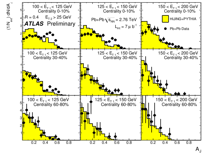
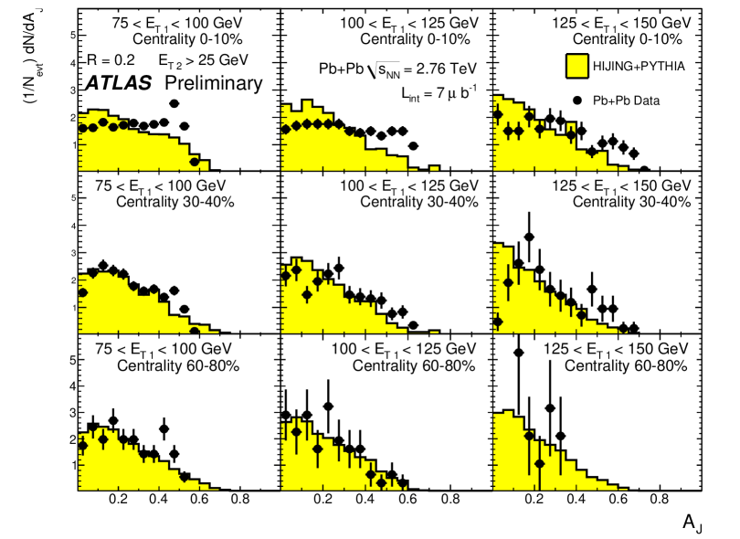
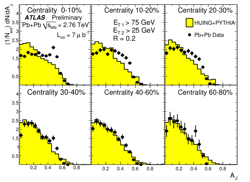
Chapter 7 Conclusion
This thesis has presented results for the jet and dijet asymmetry. The asymmetry distributions indicate that there are a class of events where there is a significant momentum imbalance between the two leading jets in the event. The extent of this imbalance gradually increases with centrality implying that the momentum balance between dijets is modified in the presence of the medium. This is strongly suggestive of the interpretation that the asymmetry is directly probing the differential energy loss of two partons traversing different in-medium path lengths. Furthermore, these dijets show an angular correlation that is consistent with vacuum dijet production. When this result was first released, the lack of modification of this angular correlation was considered surprising, especially given the copious energy loss implied by the asymmetry.
The results presented in this thesis show that jets are suppressed in central collisions by approximately a factor of two relative to peripheral collisions. This suppression is almost completely independent of . The approximate value of and the slight increase with are qualitatively consistent with predictions using the PYQUEN MC event generator [229]. As the angular size of the jets is increased, by increasing the parameter, the also increases. This -dependence of is weak and is a marginal effect above the measurement uncertainties. For lower energy jets, GeV, an increase in with that is greater than that for higher energy jets was predicted in Ref. [183], shown in Fig. 2.29. While the measurement uncertainties limit a strong conclusion, this trend is present in the data as well.
The -dependence can be compared with that of the single particle measured at the LHC shown in the summary plot in Fig. 7.1.
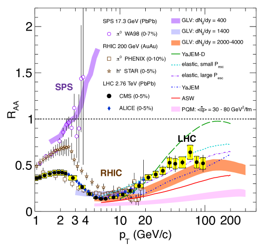
The most recent RHIC results showed a constant suppression at the highest available . The LHC results have extended to higher where the is found to rise up to , which is in the same regime as the jet shown here. While it has been argued in this thesis that there is no requirement that the single particle and jet suppression factors be related, the plateau in the -dependence exhibited by both observables suggests some common feature of the high energy loss regime.
Since the anti- jets have highly regular geometry, the parameter can be safely interpreted as a cone radius. Changing the jet radius has the effect that medium induced radiation emitted at angles between the old and new radii will be recovered by the jet and the energy loss will be reduced. An additional effect is the change in the spectral shape due to the change in definition, which is present even in the case of no quenching. Therefore, evaluations of the energy loss as a function of jet radius must be convolved with this second effect to be comparable to the experimentally observed spectra or . This is normally the case in theoretical evaluations of the or where the per parton energy loss must be convolved with the production spectrum. Equivalently, without the analogous deconvolution, a comparison between the at two radii (i.e the experimental observation in this thesis) is indirectly sensitive to the energy recovery.
A quantitative extraction of the energy loss was attempted in Ref. [224] with single particle measurements from PHENIX. The procedure used the unmodified inclusive single particle spectrum to remove the dependence on the spectral shape under the ansatz of an energy loss scenario where . In the previous chapter, this procedure was applied to fully reconstructed jets with GeV, with the extracted values providing a basis of comparison between the different values. The results of this exercise, summarized in Fig. 6.20, indicate an dependence of the energy loss that is significant beyond the estimated uncertainty. At fixed , the differences in between the two values can be interpreted as the fractional recovered energy in the annular region between the two radii. The and values remain relatively close, however increasing the radius to shows a reduction in the energy loss fraction. The marginal decrease in is even greater when moving from to . This trend indicates that the energy recovery grows faster than linearly with . The relative magnitudes of evolve with , indicating that the energy recovered by expanding the jet radius increases with .
To establish this behavior quantitatively, the dependence of was fit with the form, , with the fit results given in Table 6.1. This can be compared with the single hadron analysis performed by PHENIX. This analysis extracted larger values for than those obtained here, which is consistent with the general expectation that some of the energy radiated by the parton may be recovered when using jets. Furthermore, the was found to scale approximately as , which is consistent with the energy loss models discussed in Section 2.5.4. The values calculated here for full jets are much larger, with the 0.2, 0.3 and 0.4 jets having . The shows a slower growth.
The is only sensitive to nuclear modification effects relative to a peripheral reference spectrum in this case the 60-80% centrality bin. To quantify the full extent of these effects a reference spectrum should be used. The LHC recorded data at 2.76 TeV during early 2011, and a full measurement using this data is the obvious next step in a systematic study of jet quenching at the LHC. A jet triggered sample of approximately 150 was recorded by ATLAS, which provides ample statistics for the jet spectrum measurement out to GeV. As this reference spectrum will contain better statistics than the 60-80% Pb+Pb spectrum, the measurement can be performed in bins of rapidity as well. Since the is sensitive to the full extent of the quenching, this measurement will likely focus on the maximal suppression observed in the 0-1% or 0-5% centrality bins.
To more firmly associate the jet suppression observation with the quenching interpretation, suppression from the NPDF must be constrained through future measurements. The jet ’s tend to exhibit a decrease with increasing , particularly in the most central bins. While this effect is marginally significant beyond systematic errors, a possible explanation could be the sampling of the NPDFs in the EMC region. This scenario must be investigated; any detailed measurements of the quenching require the decomposition of the total observed suppression into contributions from cold nuclear matter effects and a quenching component. This can be checked with a measurement of the direct photon , which is sensitive to hard scattering production rates determined by the NPDFs, but not to quenching. Additionally the rates for production can be used to constrain cold nuclear matter effects, as the decay modes should also be immune to the quenching. Both ATLAS [231] and CMS [232] have published values, however these results are statistics limited and cannot provide rigorous constraints on the NPDFs. This could be improved with results from the higher statistics 2011 run. The upcoming p+Pb run at the LHC should provide an opportunity to perform full jet reconstruction in these collisions for the first time. ATLAS should not only be able to provide precision measurements for determination of the NPFs, but also measure the impact parameter-dependence of the nuclear modification effects discussed in Section 2.5.2.
In the case of photon identification, a significant background comes from ’s in jets. One of the primary techniques at rejecting this background in analyzing collisions is to require that the photon be isolated; this is typically accomplished by placing a maximum threshold on the energy deposited in a cone of fixed radius about the reconstructed photon axis, excluding the energy of the photon. The subtraction procedures developed for jet reconstruction in heavy ion collisions discussed in this thesis have been adapted by ATLAS to be applied to the isolation cones in the photon reconstruction.
As discussed previously, dijet observables provide complementary information to the single inclusive measurements as they are sensitive to the relative energy loss of the two jets. Furthermore, both gamma-jet and -jet correlations can be used in analogy with the asymmetry to determine single jet energy loss, and are considered topics of future interest. The asymmetry results presented here show that for systems with a 100 GeV leading jet, a significant fraction of events were found to have the sub-leading jet correlated in and have GeV. This means that the quenching is strong enough to regularly cause energy loss of of the jet’s energy. Furthermore, the relatively strong angular correlation indicates that this energy loss must be incurred without significantly altering the direction of the jet. Whether this feature is captured by various energy loss models is not clear, as most models used the soft eikonal limit, which does not fully describe the transverse deflection of the leading parton.
The measured angular correlation can be used to test predictions of modified acoplanarity distributions through elastic scattering [147, 148, 149]. By rescaling the -dependence by the leading jet , this quantity, defined in Eq. 2.77, can be related to the normalized dijet angular correlation,
| (7.1) |
This quantity shows almost no modification in heavy ion collisions, and significantly less modification than the predicted acoplanarity distributions, which generally show a reduction of 25-50% in the maximum of the correlation relative to .
The measured angular correlation can be used to constrain the magnitude of transverse momentum kicks, , imparted to the jet through random elastic scattering in the medium. For a dijet system with back-to-back jets with momentum before energy loss, each jet can undergo random small angle multiple scattering resulting in an RMS angular deflection of
| (7.2) |
The angular deflection of each jet is independent of the other so the effect on the dijet distribution is an additional kick of . An upper limit on can be placed by sampling the dijet distribution obtained from the MC including additional Gaussian smearing with different values of and testing to see which values are consistent with the data. Figure 7.2 shows the data along with the nominal MC distribution and several smeared variants of the MC distribution for jets with GeV in the 0-10% centrality bin. The distributions are scaled to have unit value in the highest bin to facilitate comparisons of the shapes. The distribution shown in green is clearly broader than the data, as is the distribution shown in blue except in one bin. If the former is taken as an estimate of the upper bound on and 100 GeV is used as an estimate of the jet , this corresponds to a limit of GeV.
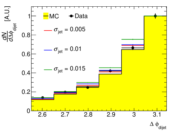
The fact that the jet suffers essentially no angular deflection means that there is a single well-defined jet axis. For events with incomplete nuclear overlap the collision zone is oblong and there are a variety of path lengths the jet could take through the same medium. Furthermore, if the overlap is assumed to have elliptical geometry, the orientation and eccentricity of the overlap region are accessible on a per event basis through the flow observables and respectively. If coordinates are chosen such that the impact parameter vector is aligned with the axis, the jet’s linear trajectory is given by , where is the angle between the jet axis and the event plane, with the primed coordinates indicating the jet production location. The geometry of this scenario is shown in Fig. 7.3. The production point of the jet is unknown on a per event basis, but the average of such positions could be taken over many collisions with the same flow characteristics.
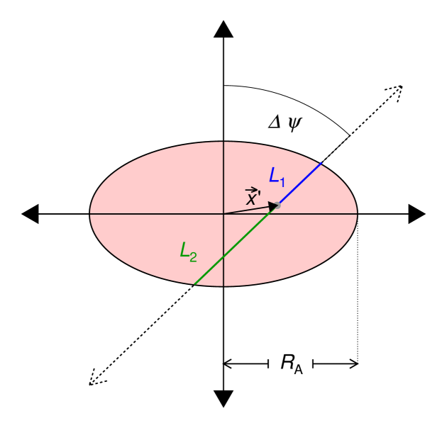
In this geometrical picture, two-jet differential and single inclusive jet observables are sensitive to different moment-like quantities in the energy loss. Consider the variable , which is some quantity sensitive to the energy loss. In a given event this should be a function of the production position, initial parton kinematics and collision geometry. The average of this variable over events of similar eccentricity and centrality should be related to the differential energy loss, integrated over all different jet production points inside an ellipse by the eccentricity,
| (7.3) |
where is the transverse density of possible jet production points. The dependence of on comes from the path length travelled in the medium, i.e. . The function can be found by determining the coordinates of the jet-ellipse intersection and computing the path length. The coordinates of where the jet leaves the medium are defined by the solutions to the simultaneous set of equations for the jet axis and the ellipse,
| (7.4) |
where is the eccentricity and is the nuclear radius which forms the semi-major axis of the ellipse. The eccentricity is assumed to be determined by centrality, but it may be possible to use per event values as an additional handle to constrain the range of eccentricity values in a class of events. Using the jet reconstruction techniques described in Chapter 4 the -integrated flow harmonics and total can be measured by excluding energy deposition associated with jets on a per event basis. This should allow better understanding of non-flow contributions to the harmonics as well as the fraction of total and particle production that comes from hard processes.
When considering the single inclusive jet energy loss, is sensitive to directly. For example, in the BDPMS-Z scheme the energy loss for a single jet is approximately , using this variable for ,
| (7.5) |
This is contrasted with the case where the dijet differential energy is the energy loss observable, . This quantity has a different dependence on the collision geometry since the path lengths of the two jets are correlated on a per event basis. Thus when averaging over similar events the quantity,
| (7.6) |
provides an independent handle on the geometrical dependence of the energy loss. If put on a more rigorous theoretical footing, calculations of these two variables in an energy loss framework would provide a testable prediction of the path length dependence. The three-jet rate is high enough at the LHC that a similar approach could be applied to events with three jets. These have additional per event geometric correlations and would provide independent moments to check the energy loss.
Relating a measured asymmetry to the partonic level energy loss can be challenging due to the intrinsic width of the vacuum asymmetry distribution. Furthermore, the distinction between multi-jet events and splitting due to hard radiation is not always clear. Some of these issues may be resolved by adding an additional step to the experimental analysis where the final jets are used as input to another round of clustering with a jet finding algorithm. For example, jets are robust against underlying event fluctuations, but are prone to more splitting than larger jet definitions. A set of jets could be used as input to a less geometrically restrictive finding such as the or Cambridge-Aachen algorithm with larger values, to build super-jet objects to be used in asymmetry-like analyses.
Jet structure and properties should also provide details on the quenching mechanism. Measurements of jet shapes as well as the transverse and longitudinal distributions of particles within jets are sensitive to the angular pattern of the medium-induced radiation. A preliminary analysis of the jet fragmentation has been presented by ATLAS [227], and a more complete study using the 2011 data set is presently underway. This analysis should provide constraints on quenching mechanism as it relates to the medium modified fragmentation functions discussed in Section 2.5.4. Although experimentally challenging, the analysis of jet fragmentation can be applied to reconstructed photons. The fragmentation photons provide an even cleaner probe of the angular radiation pattern; unlike the hadronic fragments the photons do not continue to interact with the medium after being emitted.
It is hoped that the measurements presented here will inspire theoretical calculations in the context of the various paradigms discussed in Section 2.5.4 to consider the angular dependence of the energy loss and its effect on . Comparisons can be made both in terms of radiation recovery between the different radii as well as the total amount of large angle radiation () to see whether this can give the expected total suppression of . Any plausible quenching scenario must simultaneously satisfy both of these observations.
References
- [1] Atlas Collaboration, Observation of a Centrality-Dependent Dijet Asymmetry in Lead-Lead Collisions at TeV with the ATLAS Detector at the LHC, Phys.Rev.Lett. 105 (2010) 252303, arXiv:1011.6182.
- [2] M. Han and Y. Nambu, Three Triplet Model with Double Symmetry, Phys.Rev. 139 (1965) B1006–B1010.
- [3] M. Gell-Mann, Symmetries of baryons and mesons, Phys.Rev. 125 (1962) 1067–1084.
- [4] M. Gell-Mann, A Schematic Model of Baryons and Mesons, Phys.Lett. 8 (1964) 214–215.
- [5] J. J. J. Kokkedee, The quark model, CERN-TH-757 (1967) .
- [6] G. Zweig, An model for strong interaction symmetry and its breaking: Part I, CERN-TH-401 (1964) .
- [7] G. Zweig, An model for strong interaction symmetry and its breaking: Part II, CERN-TH-412 (1964) .
- [8] V. Barnes et al., Observation of a Hyperon with Strangeness , Phys.Rev.Lett. 12 (1964) 204–206.
- [9] J. Bjorken, Asymptotic Sum Rules at Infinite Momentum, Phys.Rev. 179 (1969) 1547–1553.
- [10] E. D. Bloom et al., High-Energy Inelastic Scattering at -Degrees and -Degrees, Phys.Rev.Lett. 23 (1969) 930–934.
- [11] J. I. Friedman and H. W. Kendall, Deep inelastic electron scattering, Ann.Rev.Nucl.Part.Sci. 22 (1972) 203–254.
- [12] J. Bjorken and E. A. Paschos, Inelastic Electron-Proton and -Proton Scattering, and the Structure of the Nucleon, Phys.Rev. 185 (1969) 1975–1982.
- [13] R. P. Feynman, Very high-energy collisions of hadrons, Phys.Rev.Lett. 23 (1969) 1415–1417.
- [14] R. P. Feynman, The behavior of hadron collisions at extreme energies, Invited paper at the Third Conference on High-Energy Collisions, Stony Brook, New York, 5-6 Sep 1969 .
- [15] M. Gell-Mann and F. Low, Quantum electrodynamics at small distances, Phys.Rev. 95 (1954) 1300–1312.
- [16] K. G. Wilson, Non-Lagrangian models of current algebra, Phys.Rev. 179 (1969) 1499–1512.
- [17] C. G. Callan, Broken scale invariance in scalar field theory, Phys.Rev. D2 (1970) 1541–1547.
- [18] K. Symanzik, Small distance behavior in field theory and power counting, Commun.Math.Phys. 18 (1970) 227–246.
- [19] C. G. Callan and D. J. Gross, Bjorken scaling in quantum field theory, Phys.Rev. D8 (1973) 4383–4394.
- [20] N. H. Christ, B. Hasslacher, and A. H. Mueller, Light cone behavior of perturbation theory, Phys.Rev. D6 (1972) 3543.
- [21] C.-N. Yang and R. L. Mills, Conservation of Isotopic Spin and Isotopic Gauge Invariance, Phys.Rev. 96 (1954) 191–195.
- [22] H. Politzer, Reliable Perturbative Results for Strong Interactions?, Phys.Rev.Lett. 30 (1973) 1346–1349.
- [23] D. Gross and F. Wilczek, Ultraviolet Behavior of Non-Abelian Gauge Theories, Phys.Rev.Lett. 30 (1973) 1343–1346.
- [24] D. Gross and F. Wilczek, Asymptotically Free Gauge Theories. 1, Phys.Rev. D8 (1973) 3633–3652.
- [25] D. Gross and F. Wilczek, Asymptotically Free Gauge Theories. 2, Phys.Rev. D9 (1974) 980–993.
- [26] H. Politzer, Asymptotic Freedom: An Approach to Strong Interactions, Phys.Rept. 14 (1974) 129–180.
- [27] H. Georgi and H. Politzer, Electroproduction scaling in an asymptotically free theory of strong interactions, Phys.Rev. D9 (1974) 416–420.
- [28] S. Drell and T. Yan, Massive Lepton Pair Production in Hadron-Hadron Collisions at High-Energies, Phys.Rev.Lett. 25 (1970) 316–320.
- [29] CTEQ Collaboration, Handbook of perturbative QCD; Version 1.1: September 1994, Rev. Mod. Phys. (1994) .
- [30] K. Nakamura et al., Review of particle physics, J.Phys.G G37 (2010) 075021.
- [31] C. G. Callan and D. J. Gross, High-energy electroproduction and the constitution of the electric current, Phys.Rev.Lett. 22 (1969) 156–159.
- [32] A. Bodek et al., Experimental Studies of the Neutron and Proton Electromagnetic Structure Functions, Phys.Rev. D20 (1979) 1471–1552.
- [33] V. Ezhela, S. Lugovsky, and O. Zenin, Hadronic part of the muon g-2 estimated on the evaluated data compilation, arXiv:hep-ph/0312114.
- [34] G. Hanson et al., Evidence for Jet Structure in Hadron Production by Annihilation, Phys.Rev.Lett. 35 (1975) 1609–1612.
- [35] S. L. Wu, Physics at PETRA: The First 5-Years, Phys.Rept. 107 (1984) 59–324.
- [36] S. Bethke, The 2009 World Average of , Eur.Phys.J. C64 (2009) 689–703, arXiv:0908.1135.
- [37] L. Faddeev and V. Popov, Feynman Diagrams for the Yang-Mills Field, Phys.Lett. B25 (1967) 29–30.
- [38] G. F. Sterman and S. Weinberg, Jets from Quantum Chromodynamics, Phys.Rev.Lett. 39 (1977) 1436.
- [39] Y. L. Dokshitzer, D. Diakonov, and S. Troian, Hard Processes in Quantum Chromodynamics, Phys.Rept. 58 (1980) 269–395.
- [40] G. F. Sterman, Mass Divergences in Annihilation Processes. 1. Origin and Nature of Divergences in Cut Vacuum Polarization Diagrams, Phys.Rev. D17 (1978) 2773.
- [41] K. G. Wilson, Confinement of Quarks, Phys.Rev. D10 (1974) 2445–2459.
- [42] H. B. Nielsen and M. Ninomiya, Absence of Neutrinos on a Lattice. 1. Proof by Homotopy Theory, Nucl.Phys. B185 (1981) 20.
- [43] H. B. Nielsen and M. Ninomiya, No Go Theorem for Regularizing Chiral Fermions, Phys.Lett. B105 (1981) 219.
- [44] J. B. Kogut and L. Susskind, Hamiltonian Formulation of Wilson’s Lattice Gauge Theories, Phys.Rev. D11 (1975) 395.
- [45] K. Symanzik, Continuum Limit and Improved Action in Lattice Theories. 1. Principles and Theory, Nucl.Phys. B226 (1983) 187.
- [46] A. Bazavov et al., Nonperturbative QCD simulations with flavors of improved staggered quarks, Rev.Mod.Phys. 82 (2010) 1349–1417, arXiv:0903.3598.
- [47] Y. Nambu. Lectures at the Copenhagen symposium (1970).
- [48] T. Goto, Relativistic quantum mechanics of one-dimensional mechanical continuum and subsidiary condition of dual resonance model, Prog.Theor.Phys. 46 (1971) 1560–1569.
- [49] B. Andersson et al., Parton Fragmentation and String Dynamics, Phys.Rept. 97 (1983) 31–145.
- [50] T. Sjostrand, High-energy physics event generation with PYTHIA 5.7 and JETSET 7.4, Comput.Phys.Commun. 82 (1994) 74–90.
- [51] J. C. Collins, D. E. Soper, and G. F. Sterman, Factorization for Short Distance Hadron-Hadron Scattering, Nucl.Phys. B261 (1985) 104.
- [52] J. C. Collins, D. E. Soper, and G. F. Sterman, Soft Gluons and Factorization, Nucl.Phys. B308 (1988) 833.
- [53] J. C. Collins, D. E. Soper, and G. F. Sterman, Factorization of Hard Processes in QCD, Adv.Ser.Direct.High Energy Phys. 5 (1988) 1–91, arXiv:hep-ph/0409313.
- [54] S. J. Brodsky, D. S. Hwang, and I. Schmidt, Final-state interactions and single-spin asymmetries in semi-inclusive deep inelastic scattering, Phys.Lett. B530 (2002) 99–107, arXiv:hep-ph/0201296.
- [55] S. J. Brodsky et al., Structure functions are not parton probabilities, Phys.Rev. D65 (2002) 114025, arXiv:hep-ph/0104291.
- [56] J. C. Collins, Leading twist single transverse-spin asymmetries: Drell-Yan and deep inelastic scattering, Phys.Lett. B536 (2002) 43–48, arXiv:hep-ph/0204004.
- [57] D. Boer, P. Mulders, and F. Pijlman, Universality of -odd effects in single spin and azimuthal asymmetries, Nucl.Phys. B667 (2003) 201–241, arXiv:hep-ph/0303034.
- [58] J. C. Collins and D. E. Soper, Back-to-back jets in QCD, Nucl.Phys. B193 (1981) 381.
- [59] J. C. Collins, D. E. Soper, and G. F. Sterman, Transverse Momentum Distribution in Drell-Yan Pair and and Boson Production, Nucl.Phys. B250 (1985) 199.
- [60] J. Collins and J.-W. Qiu, factorization is violated in production of high-transverse-momentum particles in hadron-hadron collisions, Phys.Rev. D75 (2007) 114014, arXiv:0705.2141.
- [61] T. C. Rogers and P. J. Mulders, No generalized transverse momentum dependent factorization in the hadroproduction of high transverse momentum hadrons, Phys.Rev. D81 (2010) 094006, arXiv:1001.2977.
- [62] G. Altarelli and G. Parisi, Asymptotic Freedom in Parton Language, Nucl.Phys. B126 (1977) 298.
- [63] V. Gribov and L. Lipatov, Deep inelastic scattering in perturbation theory, Sov.J.Nucl.Phys. 15 (1972) 438–450.
- [64] Y. L. Dokshitzer, Calculation of the Structure Functions for Deep Inelastic Scattering and Annihilation by Perturbation Theory in Quantum Chromodynamics., Sov.Phys.JETP 46 (1977) 641–653.
- [65] A. H. Mueller, Multiplicity and Hadron Distributions in QCD Jets: Nonleading Terms, Nucl.Phys. B213 (1983) 85.
- [66] Y. L. Dokshitzer, V. A. Khoze, and S. Troian, Inclusive particle spectra from QCD cascades, Int.J.Mod.Phys. A7 (1992) 1875–1906.
- [67] Y. L. Dokshitzer, V. A. Khoze, A. H. Müller, and S. I. Troyan, Basics of perturbative QCD. Basics of. Ed. Frontières, Gif-sur-Yvette, 1991.
- [68] V. A. Khoze and W. Ochs, Perturbative QCD approach to multiparticle production, Int.J.Mod.Phys. A12 (1997) 2949–3120, arXiv:hep-ph/9701421.
- [69] C. Fong and B. Webber, One and two particle distributions at small in QCD jets, Nucl.Phys. B355 (1991) 54–81.
- [70] Y. L. Dokshitzer, V. S. Fadin, and V. A. Khoze, Double Logs of Perturbative QCD for Parton Jets and Soft Hadron Spectra, Z.Phys. C15 (1982) 325.
- [71] de Florian, Daniel and Sassot, Rodolfo and Stratmann, Marco, Global analysis of fragmentation functions for protons and charged hadrons, Phys.Rev. D76 (2007) 074033, arXiv:0707.1506.
- [72] de Florian, Daniel and Sassot, Rodolfo and Stratmann, Marco, Global analysis of fragmentation functions for pions and kaons and their uncertainties, Phys.Rev. D75 (2007) 114010, arXiv:hep-ph/0703242.
- [73] M. Hirai, S. Kumano, T.-H. Nagai, and K. Sudoh, Determination of fragmentation functions and their uncertainties, Phys.Rev. D75 (2007) 094009, arXiv:hep-ph/0702250.
- [74] B. Webber, A QCD Model for Jet Fragmentation Including Soft Gluon Interference, Nucl.Phys. B238 (1984) 492.
- [75] G. Marchesini et al., HERWIG: A Monte Carlo event generator for simulating hadron emission reactions with interfering gluons. Version 5.1 - April 1991, Comput.Phys.Commun. 67 (1992) 465–508.
- [76] S. Catani et al., QCD matrix elements + parton showers, JHEP 0111 (2001) 063, arXiv:hep-ph/0109231.
- [77] J. Alwall et al., Comparative study of various algorithms for the merging of parton showers and matrix elements in hadronic collisions, Eur.Phys.J. C53 (2008) 473–500, arXiv:0706.2569.
- [78] T. Gleisberg et al., SHERPA 1. alpha: A Proof of concept version, JHEP 0402 (2004) 056, arXiv:hep-ph/0311263.
- [79] M. L. Mangano, M. Moretti, F. Piccinini, R. Pittau, and A. D. Polosa, ALPGEN, a generator for hard multiparton processes in hadronic collisions, JHEP 0307 (2003) 001, arXiv:hep-ph/0206293.
- [80] J. E. Huth et al., Toward a standardization of jet definitions, FERMILAB-CONF-90-249-E (1990) .
- [81] S. D. Ellis, Z. Kunszt, and D. E. Soper, The One Jet Inclusive Cross-Section at Order Quarks and Gluons, Phys.Rev.Lett. 64 (1990) 2121.
- [82] G. P. Salam, Towards Jetography, Eur.Phys.J. C67 (2010) 637–686, arXiv:0906.1833.
- [83] M. Cacciari, G. P. Salam, and G. Soyez, The anti- jet clustering algorithm, JHEP 0804 (2008) 063, arXiv:0802.1189.
- [84] JADE Collaboration, Experimental Studies on Multi-Jet Production in Annihilation at PETRA Energies, Z. Phys. C33 (1986) 23.
- [85] JADE Collaboration, Experimental Investigation of the Energy Dependence of the Strong Coupling Strength, Phys. Lett. B213 (1988) 235.
- [86] S. Catani et al., New clustering algorithm for multi-jet cross-sections in annihilation, Phys.Lett. B269 (1991) 432–438.
- [87] S. Catani et al., Longitudinally invariant clustering algorithms for hadron hadron collisions, Nucl.Phys. B406 (1993) 187–224.
- [88] S. D. Ellis and D. E. Soper, Successive combination jet algorithm for hadron collisions, Phys.Rev. D48 (1993) 3160–3166, arXiv:hep-ph/9305266.
- [89] M. Cacciari and G. P. Salam, Dispelling the myth for the jet-finder, Phys.Lett. B641 (2006) 57–61, arXiv:hep-ph/0512210.
- [90] Y. L. Dokshitzer et al., Better jet clustering algorithms, JHEP 9708 (1997) 001, arXiv:hep-ph/9707323.
- [91] M. Wobisch and T. Wengler, Hadronization corrections to jet cross-sections in deep inelastic scattering, arXiv:hep-ph/9907280.
- [92] ATLAS Collaboration, Jet Reconstruction Performance, ATL-PHYS-PUB-2009-012 (2009). http://cdsweb.cern.ch/record/1167330/.
- [93] T. Kluge, K. Rabbertz, and M. Wobisch, FastNLO: Fast pQCD calculations for PDF fits, arXiv:hep-ph/0609285.
- [94] E. Fermi, High-energy nuclear events, Prog.Theor.Phys. 5 (1950) 570–583.
- [95] L. Landau, On the multiparticle production in high-energy collisions, Izv.Akad.Nauk Ser.Fiz. 17 (1953) 51–64.
- [96] R. Hagedorn, Statistical thermodynamics of strong interactions at high-energies, Nuovo Cim.Suppl. 3 (1965) 147–186.
- [97] J. C. Collins and M. Perry, Superdense Matter: Neutrons Or Asymptotically Free Quarks?, Phys.Rev.Lett. 34 (1975) 1353.
- [98] E. V. Shuryak, Quantum Chromodynamics and the Theory of Superdense Matter, Phys.Rept. 61 (1980) 71–158.
- [99] E. V. Shuryak, Two Scales and Phase Transitions in Quantum Chromodynamics, Phys.Lett. B107 (1981) 103.
- [100] M. LeBellac, Thermal Field Theory. Cambridge University Press, Cambridge, 1996.
- [101] J.-P. Blaizot and E. Iancu, The Quark gluon plasma: Collective dynamics and hard thermal loops, Phys.Rept. 359 (2002) 355–528, arXiv:hep-ph/0101103.
- [102] A. Bazavov et al., Equation of state and QCD transition at finite temperature, Phys.Rev. D80 (2009) 014504, arXiv:0903.4379.
- [103] E. Braaten and R. D. Pisarski, Soft Amplitudes in Hot Gauge Theories: A General Analysis, Nucl.Phys. B337 (1990) 569.
- [104] E. Braaten and R. D. Pisarski, Simple effective Lagrangian for hard thermal loops, Phys.Rev. D45 (1992) 1827–1830.
- [105] H. A. Weldon, Covariant Calculations at Finite Temperature: The Relativistic Plasma, Phys. Rev. D26 (1982) 1394.
- [106] A. D. Linde, Infrared Problem in Thermodynamics of the Yang-Mills Gas, Phys. Lett. B96 (1980) 289.
- [107] D. J. Gross, R. D. Pisarski, and L. G. Yaffe, QCD and Instantons at Finite Temperature, Rev. Mod. Phys. 53 (1981) 43.
- [108] T. Lee and G. Wick, Vacuum Stability and Vacuum Excitation in a Spin 0 Field Theory, Phys.Rev. D9 (1974) 2291.
- [109] T. D. Lee, Abnormal Nuclear States and Vacuum Excitations, Rev. Mod. Phys. 47 (1975) 267.
- [110] K. Rajagopal and F. Wilczek, The Condensed matter physics of QCD, arXiv:hep-ph/0011333.
- [111] J. Bjorken, Highly Relativistic Nucleus-Nucleus Collisions: The Central Rapidity Region, Phys.Rev. D27 (1983) 140–151.
- [112] PHENIX Collaboration, Measurement of the mid-rapidity transverse energy distribution from GeV Au+Au collisions at RHIC, Phys.Rev.Lett. 87 (2001) 052301, arXiv:nucl-ex/0104015.
- [113] J. M. Maldacena, The large limit of superconformal field theories and supergravity, Adv.Theor.Math.Phys. 2 (1998) 231–252, arXiv:hep-th/9711200.
- [114] O. Aharony et al., Large field theories, string theory and gravity, Phys.Rept. 323 (2000) 183–386, arXiv:hep-th/9905111.
- [115] P. Danielewicz and M. Gyulassy, Dissipative Phenomena in Quark Gluon Plasmas, Phys.Rev. D31 (1985) 53–62.
- [116] G. Policastro, D. Son, and A. Starinets, The Shear viscosity of strongly coupled supersymmetric Yang-Mills plasma, Phys.Rev.Lett. 87 (2001) 081601, arXiv:hep-th/0104066.
- [117] P. Kovtun, D. T. Son, and A. O. Starinets, Holography and hydrodynamics: Diffusion on stretched horizons, JHEP 0310 (2003) 064, arXiv:hep-th/0309213.
- [118] R.J. Glauber, in Lectures in Theoretical Physics, ed. W.E. Brittin, L.G. Dunham, 1:315. New York: Interscience (1959).
- [119] R. Glauber and G. Matthiae, High-energy scattering of protons by nuclei, Nucl.Phys. B21 (1970) 135–157.
- [120] W. Czyz and L. Maximon, High-energy, small angle elastic scattering of strongly interacting composite particles, Annals Phys. 52 (1969) 59–121.
- [121] M. L. Miller et al., Glauber modeling in high energy nuclear collisions, Ann.Rev.Nucl.Part.Sci. 57 (2007) 205–243, arXiv:nucl-ex/0701025.
- [122] H. De Vries, C. W. De Jager, and C. De Vries, Nuclear charge and magnetization density distribution parameters from elastic electron scattering, Atom. Data Nucl. Data Tabl. 36 (1987) 495–536.
- [123] A. Bialas, M. Bleszynski, and W. Czyz, Multiplicity Distributions in Nucleus-Nucleus Collisions at High-Energies, Nucl.Phys. B111 (1976) 461.
- [124] J. Cronin et al., Production of Hadrons with Large Transverse Momentum at 200 GeV, 300 GeV, and 400 GeV, Phys.Rev. D11 (1975) 3105.
- [125] D. Antreasyan et al., Production of Hadrons at Large Transverse Momentum in 200 GeV, 300 GeV and 400 GeV and p+n] Collisions, Phys.Rev. D19 (1979) 764–778.
- [126] J. W. Qiu and I. Vitev, Coherent QCD multiple scattering in proton-nucleus collisions, Phys.Lett. B632 (2006) 507–511, arXiv:hep-ph/0405068.
- [127] J. W. Qiu and G. F. Sterman, QCD and rescattering in nuclear targets, Int.J.Mod.Phys. E12 (2003) 149, arXiv:hep-ph/0111002.
- [128] A. H. Mueller and J. W. Qiu, Gluon Recombination and Shadowing at Small Values of , Nucl.Phys. B268 (1986) 427.
- [129] L. Gribov, E. Levin, and M. Ryskin, Singlet Structure Function at Small : Unitarization of Gluon Ladders, Nucl.Phys. B188 (1981) 555–576.
- [130] L. Gribov, E. Levin, and M. Ryskin, Semihard Processes in QCD, Phys.Rept. 100 (1983) 1–150.
- [131] D. F. Geesaman, K. Saito, and A. W. Thomas, The nuclear EMC effect, Ann.Rev.Nucl.Part.Sci. 45 (1995) 337–390.
- [132] L. Frankfurt and M. Strikman, Hard Nuclear Processes and Microscopic Nuclear Structure, Phys.Rept. 160 (1988) 235–427.
- [133] K. Eskola, H. Paukkunen, and C. Salgado, EPS09: A New Generation of NLO and LO Nuclear Parton Distribution Functions, JHEP 0904 (2009) 065, arXiv:0902.4154.
- [134] X. N. Wang and M. Gyulassy, HIJING: A Monte Carlo model for multiple jet production in p p, p A and A A collisions, Phys.Rev. D44 (1991) 3501–3516.
- [135] A. Capella et al., Dual parton model, Phys.Rept. 236 (1994) 225–329.
- [136] J. Ranft, Hadron production in Hadron-Nucleus and Nucleus-Nucleus Collisions in the Dual Monte Carlo Multichain Fragmentation Model, Phys.Rev. D37 (1988) 1842.
- [137] J. Ranft, Transverse Energy Distributions in Nucleus-Nucleus Collisions in the Dual Monte Carlo Multichain Fragmentation Model, Phys.Lett. B188 (1987) 379.
- [138] B. Andersson, G. Gustafson, and B. Nilsson-Almqvist, A Model for Low Hadronic Reactions, with Generalizations to Hadron-Nucleus and Nucleus-Nucleus Collisions, Nucl.Phys. B281 (1987) 289.
- [139] B. Nilsson-Almqvist and E. Stenlund, Interactions Between Hadrons and Nuclei: The Lund Monte Carlo, Fritiof Version 1.6, Comput.Phys.Commun. 43 (1987) 387.
- [140] K. Kajantie, P. Landshoff, and J. Lindfors, Minijet Production in High-Energy Nucleus-Nucleus Collisions, Phys.Rev.Lett. 59 (1987) 2527.
- [141] K. Eskola, K. Kajantie, and J. Lindfors, Quark and Gluon Production in High-Energy Nucleus-Nucleus Collisions, Nucl.Phys. B323 (1989) 37.
- [142] X. N. Wang, Role of multiple mini-jets in high-energy hadronic reactions, Phys.Rev. D43 (1991) 104–112.
- [143] J. D. Bjorken, fermilab-PUB-82/059-THY (1982).
- [144] M. H. Thoma and M. Gyulassy, Quark damping and energy loss in the high temperature QCD, Nucl.Phys. B351 (1991) 491–506.
- [145] E. Braaten and M. H. Thoma, Energy loss of a heavy quark in the quark-gluon plasma, Phys.Rev. D44 (1991) 2625–2630.
- [146] M. H. Thoma, Collisional energy loss of high-energy jets in the quark gluon plasma, Phys.Lett. B273 (1991) 128–132.
- [147] D. A. Appel, Jets as a probe of quark-gluon plasmas, Phys.Rev. D33 (1986) 717.
- [148] J. Blaizot and L. D. McLerran, Jets in expanding quark-gluon plasmas, Phys.Rev. D34 (1986) 2739.
- [149] M. Rammerstorfer and U. W. Heinz, Jet acoplanarity as a quark-gluon plasma probe, Phys.Rev. D41 (1990) 306–309.
- [150] N. Armesto et al., Comparison of Jet Quenching Formalisms for a Quark-Gluon Plasma ‘Brick’, arXiv:1106.1106.
- [151] L. Landau and I. Pomeranchuk, Limits of applicability of the theory of bremsstrahlung electrons and pair production at high-energies, Dokl.Akad.Nauk Ser.Fiz. 92 (1953) 535–536.
- [152] A. B. Migdal, Bremsstrahlung and pair production in condensed media at high-energies, Phys.Rev. 103 (1956) 1811–1820.
- [153] M. Gyulassy and M. Plumer, Jet Quenching in Dense Matter, Phys.Lett. B243 (1990) 432–438.
- [154] M. Gyulassy and X. N. Wang, Multiple collisions and induced gluon bremsstrahlung in QCD, Nucl.Phys. B420 (1994) 583–614, arXiv:nucl-th/9306003.
- [155] R. Baier, Y. L. Dokshitzer, A. H. Mueller, S. Peigne, and D. Schiff, Radiative energy loss of high-energy quarks and gluons in a finite volume quark-gluon plasma, Nucl.Phys. B483 (1997) 291–320, arXiv:hep-ph/9607355.
- [156] B. Zakharov, Fully quantum treatment of the Landau-Pomeranchuk-Migdal effect in QED and QCD, JETP Lett. 63 (1996) 952–957, arXiv:hep-ph/9607440.
- [157] R. Baier, Jet quenching, Nucl.Phys. A715 (2003) 209–218, arXiv:hep-ph/0209038.
- [158] C. A. Salgado and U. A. Wiedemann, Calculating quenching weights, Phys.Rev. D68 (2003) 014008, arXiv:hep-ph/0302184.
- [159] M. Gyulassy, P. Levai, and I. Vitev, Jet quenching in thin quark gluon plasmas. 1. Formalism, Nucl.Phys. B571 (2000) 197–233, arXiv:hep-ph/9907461.
- [160] M. Gyulassy, P. Levai, and I. Vitev, Reaction operator approach to non-Abelian energy loss, Nucl.Phys. B594 (2001) 371–419, arXiv:nucl-th/0006010.
- [161] U. A. Wiedemann, Transverse dynamics of hard partons in nuclear media and the QCD dipole, Nucl.Phys. B582 (2000) 409–450, arXiv:hep-ph/0003021.
- [162] N. Armesto et al., Medium-evolved fragmentation functions, JHEP 0802 (2008) 048, arXiv:0710.3073.
- [163] A. D. Polosa and C. A. Salgado, Jet Shapes in Opaque Media, Phys.Rev. C75 (2007) 041901, arXiv:hep-ph/0607295.
- [164] K. C. Zapp and U. A. Wiedemann, Coherent Radiative Parton Energy Loss Beyond the BDMPS-Z Limit, arXiv:1202.1192.
- [165] N. Armesto, L. Cunqueiro, and C. A. Salgado, Q-PYTHIA: A Medium-modified implementation of final state radiation, Eur.Phys.J. C63 (2009) 679–690, arXiv:0907.1014.
- [166] A. Dainese, C. Loizides, and G. Paic, Leading-particle suppression in high energy nucleus-nucleus collisions, Eur.Phys.J. C38 (2005) 461–474, arXiv:hep-ph/0406201.
- [167] C. Loizides, High transverse momentum suppression and surface effects in Cu+Cu and Au+Au collisions within the PQM model, Eur.Phys.J. C49 (2007) 339–345, arXiv:hep-ph/0608133.
- [168] K. Zapp et al., A Monte Carlo Model for ’Jet Quenching’, Eur.Phys.J. C60 (2009) 617–632, arXiv:0804.3568.
- [169] I. Lokhtin and A. Snigirev, A Model of jet quenching in ultrarelativistic heavy ion collisions and high-p(T) hadron spectra at RHIC, Eur.Phys.J. C45 (2006) 211–217, arXiv:hep-ph/0506189.
- [170] P. B. Arnold, G. D. Moore, and L. G. Yaffe, Transport coefficients in high temperature gauge theories. 1. Leading log results, JHEP 0011 (2000) 001, arXiv:hep-ph/0010177.
- [171] P. B. Arnold, G. D. Moore, and L. G. Yaffe, Photon emission from ultrarelativistic plasmas, JHEP 0111 (2001) 057, arXiv:hep-ph/0109064.
- [172] P. B. Arnold, G. D. Moore, and L. G. Yaffe, Photon emission from quark gluon plasma: Complete leading order results, JHEP 0112 (2001) 009, arXiv:hep-ph/0111107.
- [173] P. B. Arnold, G. D. Moore, and L. G. Yaffe, Photon and gluon emission in relativistic plasmas, JHEP 0206 (2002) 030, arXiv:hep-ph/0204343.
- [174] S. Jeon and G. D. Moore, Energy loss of leading partons in a thermal QCD medium, Phys.Rev. C71 (2005) 034901, arXiv:hep-ph/0309332.
- [175] S. Turbide, C. Gale, S. Jeon, and G. D. Moore, Energy loss of leading hadrons and direct photon production in evolving quark-gluon plasma, Phys.Rev. C72 (2005) 014906, arXiv:hep-ph/0502248.
- [176] Y. Mehtar-Tani, C. A. Salgado, and K. Tywoniuk, Anti-angular ordering of gluon radiation in QCD media, Phys.Rev.Lett. 106 (2011) 122002, arXiv:1009.2965.
- [177] U. A. Wiedemann, Jet quenching versus jet enhancement: a quantitative study of the BDMPS-Z gluon radiation spectrum, Nucl.Phys. A690 (2001) 731–751, arXiv:hep-ph/0008241.
- [178] W. Horowitz and B. Cole, Systematic theoretical uncertainties in jet quenching due to gluon kinematics, Phys.Rev. C81 (2010) 024909, arXiv:0910.1823.
- [179] P. B. Arnold and W. Xiao, High-energy jet quenching in weakly-coupled quark-gluon plasmas, Phys.Rev. D78 (2008) 125008, arXiv:0810.1026.
- [180] S. Caron-Huot, O(g) plasma effects in jet quenching, Phys.Rev. D79 (2009) 065039, arXiv:0811.1603.
- [181] I. Vitev, S. Wicks, and B. W. Zhang, A theory of jet shapes and cross sections: from hadrons to nuclei, JHEP 0811 (2008) 093, arXiv:0810.2807.
- [182] I. Vitev and B. W. Zhang, Jet tomography of high-energy nucleus-nucleus collisions at next-to-leading order, Phys.Rev.Lett. 104 (2010) 132001, arXiv:0910.1090.
- [183] Y. He, I. Vitev, and B. W. Zhang, Next-to-leading order analysis of inclusive jet and di-jet production in heavy ion reactions at the Large Hadron Collider, arXiv:1105.2566.
- [184] G. Ovanesyan and I. Vitev, An effective theory for jet propagation in dense QCD matter: jet broadening and medium-induced bremsstrahlung, JHEP 1106 (2011) 080, arXiv:1103.1074.
- [185] S. S. Gubser, Drag force in AdS/CFT, Phys.Rev. D74 (2006) 126005, arXiv:hep-th/0605182.
- [186] C. Herzog, A. Karch, P. Kovtun, C. Kozcaz, and L. Yaffe, Energy loss of a heavy quark moving through supersymmetric Yang-Mills plasma, JHEP 0607 (2006) 013, arXiv:hep-th/0605158.
- [187] J. Casalderrey-Solana and D. Teaney, Heavy quark diffusion in strongly coupled Yang-Mills, Phys.Rev. D74 (2006) 085012, arXiv:hep-ph/0605199.
- [188] J. Casalderrey-Solana and D. Teaney, Transverse Momentum Broadening of a Fast Quark in a Yang Mills Plasma, JHEP 0704 (2007) 039, arXiv:hep-th/0701123.
- [189] H. Liu, K. Rajagopal, and U. A. Wiedemann, Calculating the jet quenching parameter from AdS/CFT, Phys.Rev.Lett. 97 (2006) 182301, arXiv:hep-ph/0605178.
- [190] H. Liu, K. Rajagopal, and U. A. Wiedemann, Wilson loops in heavy ion collisions and their calculation in AdS/CFT, JHEP 0703 (2007) 066, arXiv:hep-ph/0612168.
- [191] N. Armesto, J. D. Edelstein, and J. Mas, Jet quenching at finite ‘t Hooft coupling and chemical potential from AdS/CFT, JHEP 0609 (2006) 039, arXiv:hep-ph/0606245.
- [192] STAR Collaboration, Centrality dependence of charged hadron and strange hadron elliptic flow from GeV Au+Au collisions, Phys.Rev. C77 (2008) 054901, arXiv:0801.3466.
- [193] ALICE Collaboration, Elliptic flow of charged particles in Pb+Pb collisions at TeV, Phys.Rev.Lett. 105 (2010) 252302, arXiv:1011.3914.
- [194] H. Song, S. A. Bass, and U. Heinz, Elliptic flow in GeV Au+Au collisions and TeV Pb+Pb collisions: insights from viscous hydrodynamics + hadron cascade hybrid model, Phys.Rev. C83 (2011) 054912, arXiv:1103.2380.
- [195] ATLAS Collaboration, Measurement of the azimuthal anisotropy for charged particle production in TeV lead-lead collisions with the ATLAS detector, arXiv:1203.3087. to appear in Phys.Rev. C.
- [196] PHENIX Collaboration, Suppression of hadrons with large transverse momentum in central Au+Au collisions at GeV, Phys.Rev.Lett. 88 (2002) 022301, arXiv:nucl-ex/0109003.
- [197] PHENIX Collaboration, Suppressed production at large transverse momentum in central Au+Au collisions at GeV, Phys.Rev.Lett. 91 (2003) 072301, arXiv:nucl-ex/0304022.
- [198] STAR Collaboration, Centrality dependence of high hadron suppression in Au+Au collisions at GeV, Phys.Rev.Lett. 89 (2002) 202301, arXiv:nucl-ex/0206011.
- [199] STAR Collaboration, Transverse momentum and collision energy dependence of high hadron suppression in Au+Au collisions at ultrarelativistic energies, Phys.Rev.Lett. 91 (2003) 172302, arXiv:nucl-ex/0305015.
- [200] STAR Collaboration, Disappearance of back-to-back high hadron correlations in central Au+Au collisions at GeV, Phys.Rev.Lett. 90 (2003) 082302, arXiv:nucl-ex/0210033.
- [201] STAR Collaboration, Distributions of charged hadrons associated with high transverse momentum particles in and Au+Au collisions at GeV, Phys.Rev.Lett. 95 (2005) 152301, arXiv:nucl-ex/0501016.
- [202] PHENIX Collaboration, Absence of suppression in particle production at large transverse momentum in GeV d+Au collisions, Phys.Rev.Lett. 91 (2003) 072303, arXiv:nucl-ex/0306021.
- [203] STAR Collaboration, Evidence from d+Au measurements for final state suppression of high hadrons in Au+Au collisions at RHIC, Phys.Rev.Lett. 91 (2003) 072304, arXiv:nucl-ex/0306024.
- [204] PHENIX Collaboration, Centrality dependence of direct photon production in GeV Au+Au collisions, Phys.Rev.Lett. 94 (2005) 232301, arXiv:nucl-ex/0503003.
- [205] K. Reygers, Characteristics of Parton Energy Loss Studied with High- Particle Spectra from PHENIX, J.Phys.G G35 (2008) 104045, arXiv:0804.4562.
- [206] e. Evans, Lyndon and e. Bryant, Philip, LHC Machine, JINST 3 (2008) S08001.
- [207] G. P. Jackson, A dedicated hadronic B-factory: Accelerator considerations, Nucl. Instrum. Meth. A408 (1998) 296–307.
- [208] R. Bailey and P. Collier, Standard Filling Schemes for Various LHC Operation Modes, LHC-PROJECT-NOTE-323 , http://cdsweb.cern.ch/record/691782.
- [209] ATLAS Collaboration, The ATLAS Experiment at the CERN Large Hadron Collider, JINST 3 (2008) S08003.
- [210] ATLAS Collaboration, Drift Time Measurement in the ATLAS Liquid Argon Electromagnetic Calorimeter using Cosmic Muons, Eur.Phys.J. C70 (2010) 755–785, arXiv:1002.4189.
- [211] ATLAS Collaboration, Measurement of the pseudorapidity and transverse momentum dependence of the elliptic flow of charged particles in lead-lead collisions at TeV with the ATLAS detector, Phys.Lett. B707 (2012) 330–348, arXiv:1108.6018.
- [212] S. Agostinelli et al., GEANT4: A Simulation toolkit, Nucl.Instrum.Meth. A506 (2003) 250–303.
- [213] J. Allison et al., GEANT4 developments and applications, IEEE Trans.Nucl.Sci. 53 (2006) 270.
- [214] ATLAS Collaboration, The ATLAS Simulation Infrastructure, Eur.Phys.J. C70 (2010) 823–874, arXiv:1005.4568.
- [215] M. Masera et al., Anisotropic transverse flow introduction in Monte Carlo generators for heavy ion collisions, Phys. Rev. C79 (2009) 064909.
- [216] ATLAS Collaboration, Jet energy measurement with the ATLAS detector in proton-proton collisions at TeV, arXiv:1112.6426. to appear in Eur.Phys.J. C.
- [217] ATLAS Collaboration, Centrality Determination in the 2010 Pb+Pb physics data, ATL-COM-PHYS-2011-427 (2011).
- [218] ATLAS Collaboration, Transverse energy fluctuations in Pb+Pb collisions at TeV with the ATLAS detector at the LHC, ATLAS-CONF-2012-045 (2012). http://cdsweb.cern.ch/record/1440894.
- [219] ATLAS Collaboration, Overlay for ATLAS Simulation, ATL-SOFT-INT-2011-001 (2011).
- [220] A. Hocker and V. Kartvelishvili, SVD approach to data unfolding, Nucl. Instrum. Meth. A372 (1996) 469–481.
- [221] RooUnfold. http://hepunx.rl.ac.uk/ adye/software/unfold/RooUnfold.html.
- [222] JetEnergyResolutionProvider. https://twiki.cern.ch/twiki/bin/view/Main/JetEnergyResolutionProvider.
- [223] ATLAS Collaboration, Jet Energy Resolution and Selection Efficiency Relative to Track Jets from In-situ Techniques with the ATLAS Detector Using Proton-Proton Collisions at a Center of Mass Energy TeV, ATLAS-CONF-2010-054 (2010). http://cdsweb.cern.ch/record/1281311.
- [224] PHENIX Collaboration, Formation of dense partonic matter in relativistic nucleus-nucleus collisions at RHIC: Experimental evaluation by the PHENIX collaboration, Nucl.Phys. A757 (2005) 184–283, arXiv:nucl-ex/0410003.
- [225] B. A. Cole, Jet probes of TeV Pb+Pb collisions with the ATLAS detector, J.Phys.G G38 (2011) 124021.
- [226] A. Angerami, Measurement of Jets and Jet Suppression in TeV Lead-Lead Collisions with the ATLAS detector at the LHC, J.Phys.G G38 (2011) 124085, arXiv:1108.5191.
- [227] ATLAS Collaboration, Centrality dependence of Jet Yields and Jet Fragmentation in Lead-Lead Collisions at TeV with the ATLAS detector at the LHC, ATLAS-CONF-2011-075 (2011). http://cdsweb.cern.ch/record/1353220.
- [228] ATLAS Collaboration, Measurement of inclusive jet and dijet cross sections in proton-proton collisions at 7 TeV centre-of-mass energy with the ATLAS detector, Eur.Phys.J. C71 (2011) 1512.
- [229] e. Armesto, N., e. Borghini, N., e. Jeon, S., e. Wiedemann, U.A., S. Abreu, et al., Heavy Ion Collisions at the LHC - Last Call for Predictions, J.Phys.G G35 (2008) 054001, arXiv:0711.0974.
- [230] CMS Collaboration, Study of high- charged particle suppression in Pb+Pb compared to collisions at TeV, arXiv:1202.2554.
- [231] ATLAS Collaboration, Measurement of the centrality dependence of yields and observation of production in lead-lead collisions with the ATLAS detector at the LHC, Phys.Lett. B697 (2011) 294–312, arXiv:1012.5419.
- [232] CMS Collaboration, Study of boson production in Pb+Pb collisions at nucleon-nucleon centre of mass energy TeV, Phys.Rev.Lett. 106 (2011) 212301, arXiv:1102.5435.