Probability of Failure in Hypersonic Engines Using Large Deviations

Abstract

We consider a reduced order model of an air-breathing hypersonic engine with a time-dependent stochastic inflow that may cause the failure of the engine. The probability of failure is analyzed by the Freidlin-Wentzell theory, the large deviation principle for finite dimensional stochastic differential equations. We compute the asymptotic failure probability by numerically solving the constrained optimization related to the large deviation problem. A large-deviation-based importance sampling suggested by the most probable inflow perturbation is also implemented to compute the probability of failure of the engine. The numerical simulations show that the importance sampling method is much more efficient than the basic Monte Carlo method.

1 Introduction

Operation of a scramjet (supersonic combustion ramjet) is difficult to accurately model with state-of-the-art codes due to the complex physical and chemical systems governing the flow of air through and the combustion in the engine. When coupled with environmental uncertainties, a priori design of a safety, high-performance operation plan (fuel schedule) is a lofty ambition. This paper numerically analyzes the probability of failure for a scaled engine operating at about Mach $2$. While there are many uncertainties outside of the engine that can effect the operability, we focus only on those within the core engine-system: the isolator, combustor and nozzle. The combustor is the location of the most complex (and least certain) chemistry: the amount of heat released here directly effects the performance of the system.

Thermal choking can result from excessive fueling, which decreases immediate performance and produces a shock that may travel through the isolator. If the shock reaches the entrance of the isolator, the engine will stall; this is called unstart. While there are many other causes of unstart (for example, thermal deformation of the engine [1]), we focus on the unstart directly related to the inflow perturbations [11] and the fueling of the engine. Iaccarino et al [5] studied the relationship between the amount of heat released and the operability of the engine over short time scales and with a low-fidelity model of the stochastic nature of the fueling. This paper studies the resulting uncertainty of the flow in the engine with a stochastic inflow Mach number.

The Euler equations are frequently employed to model compressible flows in aerospace models, especially in steady-state as a numerically tractable model when designing airfoils (see [6]). The time-dependent, quasi-one-dimensional form of the equations can be used to capture the geometry of a compression-expansion engine (see e.g. [12]) and replicates many of the physical features of actual flows in scramjet engines. When used to model scramjets, a forcing term is added that models the heat release mechanism of fueling. It is well documented that these models capture the physical shock that results from thermal choking. Due to the one-dimensional nature of these equations, they can be solved quickly and are ideal as a reduced order model.

The large deviation principle is used to analyze events with exponentially small probability. The Freidlin-Wentzell theory, the large deviation principle for finite dimensional stochastic differential equations is the mathematical tool to compute the probability of failure: when the random perturbation in the stochastic differential equation is small, the probability of failure decreases exponentially fast and the rate of decay of the probability is governed by the minimum of the rate function over the event of interest. We numerically solve this constrained optimization problem to obtain the asymptotic probability of failure and the most probable path causing unstart under several interesting cases. This so-called the minimum action method has been successfully applied to different model problems (see [4, 16]).

Another obvious way to compute the probability of unstart is to use the Monte Carlo simulations. It has been extensively used in the engineering community to consider more elaborate scramjet models such as the two-dimensional model with the second order discretization, and it can be accelerated by using the adjoint-based sampling method [14]. When the targeted probability is small, however, because of the natural limitation of the basic Monte Carlo method, one needs a excessively large number of samples to accurately estimate the probability, and such large amount of computations leads to the inefficiency of the basic Monte Carlo method. We use the large-deviation-based importance sampling technique, the importance sampling Monte Carlo method whose change of measure based on the minimizer of the large deviation principle. Our numerical results show that the large-deviation-based importance sampling outperforms the basic Monte Carlo method.

This paper is organized as follows: in Section 2 we discuss the equations that govern the flow, the geometry of the engine and the definition of the unstart; Section 3 briefly introduces the classical Freidlin-Wentzell theory, the large deviation principle for finite dimensional stochastic differential equations, and the large deviations for the related Euler schemes. In Section 4, we explain how to formulate the unstart of the scramjet as a large deviation problem. Section 5 shows the numerical results of the large deviation problems in Section 4 under different settings. In Section 6 we use the importance sampling Monte Carlo method based on the solution of the large deviation problems in Section 5 to directly estimate the probability of the unstart. Section 7 concludes this paper. The table of parameters and the numerical PDE method for the governing equation are in the appendices.

2 Model Problem

2.1 Governing Equations and Engine Geometry

The quasi-1D compressible Euler equations serve as our reduced model of the engine-combustion system and capture the phenomena of unstart due to fueling. This model was developed by Iaccarino et al [5] and is similar to the model developed by Bussing and Murmam [2]. The quasi-1D compressible Euler equations are the following hyperbolic system:

$$\begin{pmatrix}\rho\\ \rho u\\ E\\ \end{pmatrix}_{t}+\begin{pmatrix}\rho u\\ \rho u^{2}+P\\ (E+P)u\\ \end{pmatrix}_{x}=\frac{A^{\prime}(x)}{A(x)}\left(\begin{pmatrix}0\\ P\\ 0\\ \end{pmatrix}-\begin{pmatrix}\rho u\\ \rho u^{2}+P\\ (E+P)u\\ \end{pmatrix}\right)+\begin{pmatrix}0\\ 0\\ f(x,t)\\ \end{pmatrix},$$ (1)

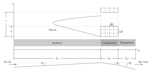
where $\rho$ is the density of the fluid, $\rho u$ is the momentum and $E$ is the total energy. The pressure $P$ can be derived from an equation of state and we take $P=(\gamma-1)(E-\rho u^{2}/2)$ where $\gamma$ is the ratio of specific heats, taken to be $1.4$. The function $A(x)$ describes the cross-sectional area of the engine; we assume that the width is constant and thus the area varies as the height; see Figure 1 for a sample height profile and the following mathematical definition:

$$A(x)=\begin{cases}A_{0}-x\sin\theta_{I},&-L_{I}<x<0,\\ A_{0}+x\sin\theta_{C},&0\leq x\leq L_{C},\\ A_{0}+L_{C}\sin\theta_{C}+(x-L_{c})\sin\theta_{E},&L_{C}<x\leq L_{C}+L_{E}.\end{cases}$$

The term $f(x,t)$ models the heat release due to fueling and takes the form:

$$f(x,t)=\begin{cases}f(t)f(x)\cdot\phi\cdot f_{stoch}\cdot H_{prop}\cdot A_{0}\cdot\rho_{0}\cdot u_{0}/(L^{2}_{C}\cdot A(x)),&x\in[0,L_{C}],\\ 0,\quad&\text{otherwise.}\end{cases}$$ (2)

where $f(x)=x^{1/3}$ following Iaccarino et al [5] and Riggins et al [10] and O’Byrne et al [8]. $\phi$ is the equivalence ratio and governs the amount of heat released into the system per unit time and $f(t)$ is an indicator for when the engine is fueling.

Fig. 1: Geometry of 1D engine model. This figure is a schematic of both the engine geometry (shown in the lower half of the image) and of the fueling profile and a resulting shock. $L_{I}$, $L_{C}$ and $L_{E}$ are the lengths of the isolator, combustor and expansion region; $\theta_{I}$, $\theta_{C}$ and $\theta_{E}$ are their respective angles; the air flows in from the left and out at the right. In the top half, the $x$ axis gives the location in the engine and the $y$ axis is time. $T$ is the full length of a fueling period and $b$ is the burst length.

2.2 Unstart of the Engine

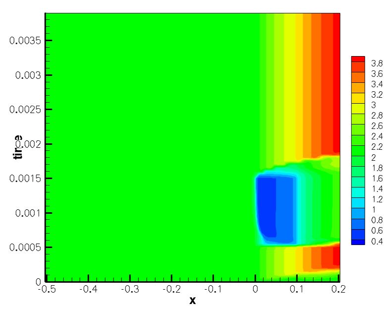
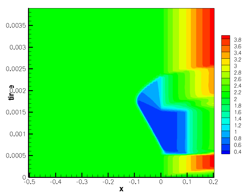
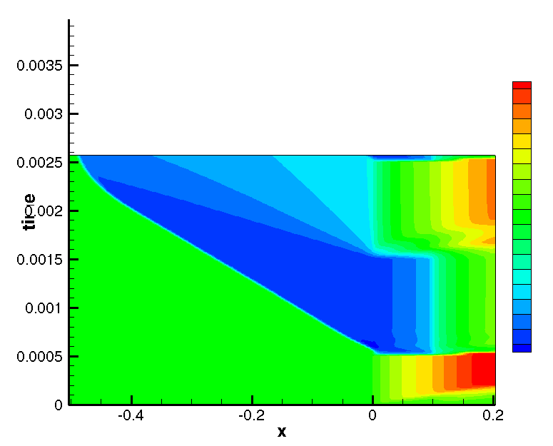
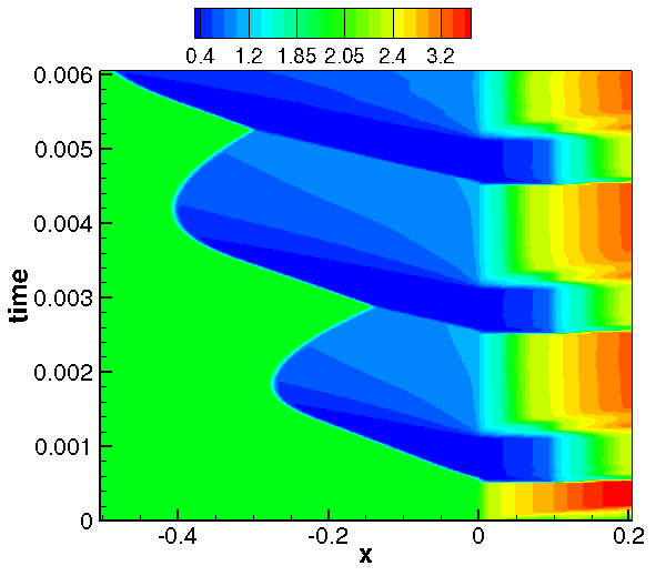
The Mach number, defined as $M=u/\sqrt{\gamma P/\rho}$, characterizes the behavior of the flow. The Mach number of the flow is plotted Figures 2(a)-2(d) for different values of $\phi$, when the engine is fueled from $t=0.5$ms to $t=1.5$ms. In all cases a shock develops, from a supersonic Mach number (Mach 2, green) to a subsonic Mach number (0.4, blue). This shock extends into the isolator of the engine and persists after the fueling has stopped. The distance into the isolator that the shock travels before receding and the amount of time it takes for the engine to return to a “normal” idle state are functions of how much head is injected. In Figure 2(d) the shock reaches the left boundary of the inlet; this is called “unstart” and the engine has failed and ceases to produce thrust. To determine if the engine has unstarted, the shock location, defined as:

$$x_{shock}=\sup\{x\in[-L_{c},0]:M(x)\geq 1\},$$

is tracked. When the engine is in a idle state $x_{shock}=0$; when the engine has failed $x_{shock}=-L_{c}$.

(a) Low Fueling Rate

(b) Moderate Fueling Rate

(c) Excessive/Stalling

(d) Compounding Shock

Fig. 2: Effect of heat release parameters on deterministic solutions of Mach number. (a)-(c):Inflow Mach number = 2.0, $b=1$ms. Progressing from (a) to (c), more head is added per unit time, driving the shock further into the isolator. In (d), where the shock reaches the left boundary, the engine stalls; this is called unstart. (d) Here, $T/b=3.33$; the bursts are not spaced sufficiently far apart, and the location of the shock compounds.

2.3 Heat Release Model

With this simplified model, there are two regimes of operation depending on $\phi$: for sufficiently small $\phi$ (Figure 2(a)) the shock does not leave the combustor, however insufficient thrust is produced; for $\phi$ greater than a threshold value $\phi^{*}\approx 0.25$, a shock forms in the isolator and will propagate until the engine unstarts. This suggests that the simplest heat-release program that could result in sustained operation of the engine is to inject heat periodically. In this paper $f(t)$ is defined as follows:

$$f(t)=\begin{cases}1,&t\in[n\tau,n\tau+b),\\ 0,&t\in[n\tau+b,(n+1)\tau).\end{cases}$$

where $\tau$ is the length of the fuel cycle and $b$ is the length of the fuel burst (the amount of time fuel is being injected into the engine). With this heat release model, a potential cause of unstart is not spacing the fuel burst sufficiently far apart ($\tau/b$ too small) which causes the shock to build upon itself and eventually leads to unstart, see Figure 2(d).

The instantaneous thrust produced by the engine is given by

$$\mathrm{thrust}(t)=\dot{m}_{e}u_{e}-\dot{m}_{i}u_{i}+(P_{e}-P_{i})A_{e}=(A\rho u^{2})_{e}-(A\rho u^{2})_{i}+(P_{e}-P_{i})A_{e},$$

where the index $e$ is for quantities at the exit of the engine and $i$ if for quantities at the front of the inlet. The mass flow, $\dot{m}$, is given by the state variable $\rho u$. When the engine is stalled no additional thrust is produced. The thrust produce is proportional to the amount of heat injected.

Depending on the extensive numerical experiments in [15], two fueling profiles are used in this paper: $\phi_{S}=0.78$, $\tau_{S}=0.5$ms, $b_{S}=0.1$ms (the short fuel cycle) and $\phi_{L}=0.78$, $\tau_{L}=2$ms, $b_{L}=0.4$ms (the long fuel cycle). Note that because $\phi_{S}=\phi_{L}$ and $\tau_{S}/b_{S}=\tau_{L}/b_{L}=5$, these two fueling profiles release the same amount of the heat so they generate roughly the same amount of thrust.

2.4 Inflow Uncertainty and Its Effect on Unstart

There are many sources of uncertainty that contribute to the total uncertainty in the operability of the scramjet engine. Those specific to the engine are the geometry (due to manufacturing errors or imperfections), the ratio of specific heats $\gamma$, the inflow conditions (the Mach number, density and pressure of air entering the engine) and the combustion processes. In this paper we only address the uncertainty of the inflow Mach number $M_{in}(t)$ that is modeled as:

$$M_{in}(t)=M_{in}(0)+\epsilon\sigma_{M}W_{t}$$ (3)

with the initial condition $M_{in}(0)=2$, where $\epsilon$ and $\sigma$ are positive constants and $W_{t}$ is the standard Brownian motion. In addition, we assume that the inflow density $\rho_{in}(t)$ and the inflow pressure $P_{in}(t)$ are constant in time. Then the perturbation of $M_{in}(t)$ completely comes from the perturbation of the inflow speed $u_{in}(t)$

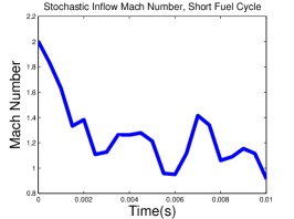
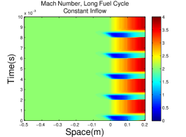
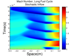
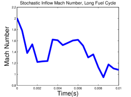
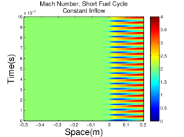
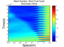
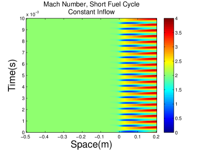
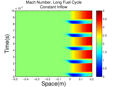
The inflow uncertainty can greatly affect the stability of the screamjet even though it operas normally under steady inflows. As shown in Figure 3, if the aforementioned fueling profiles are used (the short and long fuel cycles) and $M_{in}(t)=M_{in}(0)$ ($\epsilon\sigma=0$), the scramjet operates normally. However, if stochastic inflows are used ($\epsilon\sigma\neq 0$), then the inflow may affect the locations of the shocks and therefore the probability of the unstart is nonzero.

Fig. 3: Effects of the inflow uncertainty on the scramjet stability. The left figures are the Mach numbers in the engine with constant inflow (Mach $2$). The engine operates normally under both fueling profiles (the short and long cycles) because the subsonic flows do not reach the left boundary. After replacing the steady inflows by stochastic ones (shown in the right figures), however, the shock locations are affected by the inflow and reach the left boundary so the unstart happens (shown in the middle figures).

In this paper, the primary goal is to consider the probability of the unstart due to the stochastic inflow modeled as (3). We are especially interested in the case that the parameter $\epsilon$ in (3) is a small positive value, which lead to the large deviation analysis in the next section.

3 Large Deviation Principle

In this section, we first briefly review the classical Freidlin-Wentzell theory, the large deviation principle (LDP) for the stochastic differential equation. Then the analogous LDP for the Euler scheme of the discrete problem is introduced. The discrete problem provides a good understanding of the LDP for our unstart problem in the next section.

3.1 The Freidlin-Wentzell Theory

We consider the following stochastic differential equation (SDE):

$$dX_{t}^{\epsilon}=\alpha(X_{t}^{\epsilon})dt+\epsilon\sigma dW_{t},$$ (4)

where $X_{0}^{\epsilon}=x_{0}$ is deterministic, $W_{t}$ is the standard Brownian motion, and $\epsilon$ and $\sigma$ are positive constants. The standard theorem says that there exists a unique strong solution on any finite time interval $\left[0,T\right]$ if $\alpha:\mathbb{R}\to\mathbb{R}$ is uniformly Lipschitz continuous (see, for example, [9]). We assume that $\bar{X}_{t}$ on $[0,T]$ with $\bar{X}_{0}=x_{0}$ is the unique solution of the following differential equation:

$$\frac{d}{dt}\bar{X}_{t}=\alpha(\bar{X}_{t}).$$

It is well-known that as $\epsilon\to 0$, $X_{t}^{\epsilon}$ converges to $\bar{X}_{t}$ in probability, that is, for any $\delta>0$,

$$\lim_{\epsilon\to 0}\mathbb{P}\left(\max_{t\in[0,T]}|X_{t}^{\epsilon}-\bar{X}_{t}|>\delta\right)=0.$$

The Freidlin-Wentzell theory says that as $\epsilon\to 0$, the asymptotic probability that $X_{t}^{\epsilon}$ deviates from $\bar{X}_{t}$ can be computed as follows:

$$-\inf_{x_{t}\in\mathring{\mathcal{A}}}\mathcal{I}(x_{t}) \leq\liminf_{\epsilon\to 0}\frac{1}{\epsilon^{2}}\log\mathbb{P}(X_{t}^{\epsilon}\in\mathcal{A})$$

$$\leq\limsup_{\epsilon\to 0}\frac{1}{\epsilon^{2}}\log\mathbb{P}(X_{t}^{\epsilon}\in\mathcal{A})\leq-\inf_{x_{t}\in\bar{\mathcal{A}}}\mathcal{I}(x_{t}),$$

where the rare event $\mathcal{A}$ is any subset of $C_{x_{0}}([0,T])$, the space of continuous paths on $[0,T]$ with the starting point $x_{0}$ endowed with the standard topology. $\mathring{\mathcal{A}}$ and $\bar{\mathcal{A}}$ stand for the interior and closure of $\mathcal{A}$, respectively. The rate function $\mathcal{I}$ measures how much $X_{t}$ deviates from its typical behavior in the $L^{2}$ sense:

$$\mathcal{I}(x_{t})=\begin{cases}\frac{1}{2\sigma^{2}}\int_{0}^{T}[\frac{d}{dt}x_{t}-\alpha(x_{t})]^{2}dt,&x_{t}=x_{0}+\int_{0}^{t}y(s)ds,~{}y\in L^{2}([0,T]),\\ +\infty,&\text{otherwise.}\end{cases}$$

Remark. For the proof of the Freidlin-Wentzell theory, readers may refer to [3, Section 5.6]. In fact, the complete version of the Freidlin-Wentzell theory works for any finite dimensional SDEs and $\sigma$ can be a function of $X_{t}$. However, because we simply model the inflow Mach number as a Brownian motion, we use the current version to keep the expression of the rate function simple.

An immediate observation is that if $\mathcal{A}$ is regular, that is,

$$\inf_{x_{t}\in\mathring{\mathcal{A}}}\mathcal{I}(x_{t})=\inf_{x_{t}\in\mathcal{A}}\mathcal{I}(x_{t})=\inf_{x_{t}\in\bar{\mathcal{A}}}\mathcal{I}(x_{t}),$$

then we can represent the asymptotic probability in the following way:

$$\mathbb{P}(X_{t}^{\epsilon}\in\mathcal{A})\sim\exp\left(-\frac{1}{\epsilon^{2}}\inf_{x_{t}\in\mathcal{A}}\mathcal{I}(x_{t})\right)$$

for small $\epsilon$. In addition, if $\bar{X}_{t}\in\mathcal{A}$, then $\mathbb{P}(X_{t}^{\epsilon}\in\mathcal{A})\sim 1$ as $\epsilon\to 0$. Indeed, because $X_{t}^{\epsilon}\to\bar{X}_{t}$ as $\epsilon\to 0$, any regular event containing $\bar{X}_{t}$ should be of probability one as $\epsilon\to 0$.

3.2 Large Deviations for the Euler Scheme

For the computational purpose, one can use the Freidlin-Wentzell theory to obtain the analytical rate function, then discretizes the rate function and the functional space, and finally obtains the probability by solving the numerical optimization. However, it is more informative to consider the discrete problem by the Euler method and derive the exact LDP for the discrete problem. Then this LDP can be solved directly by the numerical optimization.

We consider the following difference equation by the Euler scheme:

$$X_{n+1}^{\epsilon}=X_{n}^{\epsilon}+\alpha(X_{n}^{\epsilon})\Delta t+\epsilon\sigma\Delta W_{n+1},$$ (5)

where $X_{0}^{\epsilon}=x_{0}$ is deterministic, $\{\Delta W_{n+1}\}_{n=0}^{N-1}$ are independent Gaussian random variables with mean zero and variance $\Delta t$, and $\epsilon>0$. We assume that $T=N\Delta t$. The joint density $p$ of $(X_{1}^{\epsilon},\ldots,X_{N}^{\epsilon})$ can be derived by the Markov property:

$$p(X_{N}^{\epsilon}=x_{N},\ldots,X_{1}^{\epsilon}=x_{1})=\prod_{n=0}^{N-1}h(X_{n+1}^{\epsilon}=x_{n+1}|X_{n}^{\epsilon}=x_{n})$$

$$\quad=\prod_{n=0}^{N-1}\frac{1}{\sqrt{2\pi\epsilon^{2}\sigma^{2}\Delta t}}\exp\left(-\frac{1}{2\epsilon^{2}\sigma^{2}\Delta t}(x_{n+1}-x_{n}-\alpha(x_{n})\Delta t)^{2}\right)$$

$$\quad=(2\pi\epsilon^{2}\sigma^{2}\Delta t)^{-N/2}\exp\left(-\frac{\Delta t}{2\epsilon^{2}\sigma^{2}}\sum_{n=0}^{N-1}\left(\frac{x_{n+1}-x_{n}}{\Delta t}-\alpha(x_{n})\right)^{2}\right).$$

Let $x=(x_{1},\ldots,x_{N})$ and

$$I(x)=\frac{\Delta t}{2\sigma^{2}}\sum_{n=0}^{N-1}\left(\frac{x_{n+1}-x_{n}}{\Delta t}-\alpha(x_{n})\right)^{2}.$$

Then given a set $\mathbf{A}\subset\mathbb{R}^{N}$ the probability that $(X_{1}^{\epsilon},\ldots,X_{N}^{\epsilon})\in\mathbf{A}$ is

$$\mathbb{P}((X_{1}^{\epsilon},\ldots,X_{N}^{\epsilon})\in\mathbf{A})=\int_{\mathbf{A}}(2\pi\epsilon^{2}\sigma^{2}\Delta t)^{-N/2}\exp\left(-\frac{1}{\epsilon^{2}}I(x)\right)dx.$$ (6)

We use Laplace’s method to compute the asymptotic probability as $\epsilon\to 0$. The basic idea is that as $\epsilon\to 0$, the mass of the integrand in (6) will concentrate at its maximizer, which is the minimizer of $I$. We can therefore use the minimum to compute the probability.

Theorem 1.

(Laplace’s method) Assume that $x^{*}=\arg\min_{x\in\mathbf{A}}I(x)$ with $x^{*}\in\mathring{\mathbf{A}}$, and $I(x)$ grows at least quadratically. Then

$$\lim_{\epsilon\to 0}\epsilon^{2}\log\mathbb{P}((X_{1}^{\epsilon},\ldots,X_{N}^{\epsilon})\in\mathbf{A})=-I(x^{*}).$$

Proof.

Because $I(x)$ grows at least quadratically, for any $\delta>0$, we can find a sufficiently large ball $B_{d}=\{x\in\mathbb{R}^{N}:\|x\|\leq d\}$ such that

$$\int_{B_{d}^{C}}(2\pi\epsilon^{2}\Delta t)^{-N/2}\exp\left(-\frac{1}{\epsilon^{2}}I(x)\right)dx<\delta$$

for all sufficiently small $\epsilon$. To compute the upper bound, it hence suffices to prove the case that $\mathbf{A}$ is bounded. We rewrite the integral as

$$\exp\left(-\frac{1}{\epsilon^{2}}I(x^{*})\right)\int_{\mathbf{A}}(2\pi\epsilon^{2}\Delta t)^{-N/2}\exp\left(-\frac{1}{\epsilon^{2}}[I(x)-I(x^{*})]\right)dx.$$

The upper bound is

$$\epsilon^{2}\log\mathbb{P}((X_{1}^{\epsilon},\ldots,X_{N}^{\epsilon})\in\mathbf{A})$$

$$\quad=-I(x^{*})+\epsilon^{2}\log(2\pi\epsilon^{2}\Delta t)^{-N/2}+\epsilon^{2}\log\int_{\mathbf{A}}\exp\left(-\frac{1}{\epsilon^{2}}[I(x)-I(x^{*})]\right)dx$$

$$\quad\leq-I(x^{*})+\epsilon^{2}\log(2\pi\epsilon^{2}\Delta t)^{-N/2}+\epsilon^{2}\log|\mathbf{A}|.$$

Then we have the upper bound of the limit

$$\lim_{\epsilon\to 0}\epsilon^{2}\log\mathbb{P}((X_{1}^{\epsilon},\ldots,X_{N}^{\epsilon})\in\mathbf{A})\leq-I(x^{*}).$$

To show the lower bound, we use the assumption that $x^{*}\in\mathring{\mathbf{A}}$. By the continuity of $I$, for any $\delta>0$, there exists a neighborhood $N_{\delta}\subset\mathring{\mathbf{A}}$ of $x^{*}$ such that $0\leq I(x)-I(x^{*})\leq\delta$ for $x\in N_{\delta}$. Then we have the lower bound:

$$\epsilon^{2}\log\mathbb{P}((X_{1}^{\epsilon},\ldots,X_{N}^{\epsilon})\in\mathbf{A})\geq\epsilon^{2}\log\mathbb{P}((X_{1}^{\epsilon},\ldots,X_{N}^{\epsilon})\in N_{\delta})$$

$$\quad=-I(x^{*})+\epsilon^{2}\log(2\pi\epsilon^{2}\Delta t)^{-N/2}+\epsilon^{2}\log\int_{N_{\delta}}\exp\left(-\frac{1}{\epsilon^{2}}[I(x)-I(x^{*})]\right)dx$$

$$\quad\geq-I(x^{*})+\epsilon^{2}\log(2\pi\epsilon^{2}\Delta t)^{-N/2}+\epsilon^{2}\log(-|N_{\delta}|\frac{\delta}{\epsilon^{2}}).$$

Therefore the lower bound is also obtained:

$$\lim_{\epsilon\to 0}\epsilon^{2}\log\mathbb{P}((X_{1}^{\epsilon},\ldots,X_{N}^{\epsilon})\in\mathbf{A})\geq-I(x^{*}).$$

∎

Readers can find that $I(x)\to\mathcal{I}(x_{t})$ as $\Delta t\to 0$. In fact, the following lemma says that $X^{\epsilon}_{n}$ is an exponentially good approximation of $X^{\epsilon}_{t}$.

Lemma 2.

(Exponential equivalence [3, Lemma 5.6.9]) If $W_{t}$ in (4) and $\Delta W_{n+1}$ in (5) satisfy

$$\Delta W_{n+1}=\int_{n\Delta t}^{(n+1)\Delta t}dW_{s}=W_{(n+1)\Delta t}-W_{n\Delta t}$$

almost surely, then for any $\delta>0$,

$$\lim_{\Delta t\to 0}\limsup_{\epsilon\to 0}\log\mathbb{P}\left(\max_{n}\sup_{t\in[n\Delta t,(n+1)\Delta t]}|X^{\epsilon}_{t}-X^{\epsilon}_{n}|>\delta\right)=-\infty.$$

Lemma 2 also tells us that we can effectively simulate a rare event by the Euler method. The standard theory shows that the Euler method has the order of accuracy $\sqrt{\Delta t}$; however, by the large deviations, the probability of a rare event is of order $\exp(-1/\epsilon^{2})$ for small $\epsilon$. Therefore we might need to decrease $\Delta t$ exponentially in $\epsilon$ to obtain the correct simulation, and such exponential discretization will make the simulation computationally impossible. Thanks to Lemma 2, we only need to choose a uniform $\Delta t$ and the Euler method can accurately simulate a rare event for all small $\epsilon$.

4 Large Deviations for the Unstart

In this section, we derive the large deviation principle for the unstart of the scramjet. First we formulate the analytical problem. Readers can immediately identify that the analytical problem is an application of the Freidlin-Wentzell theory. However, as this problem can only be solved numerically, we also need the LDP for the discretized problem. In other words, we derive the LDP for the numerical PDE of the flow equation. The readers can also find that the theory is almost ready because of the derivation in the last section.

4.1 Analytical Model

Recall that the flow equation in the scramjet engine is

$$\begin{pmatrix}\rho\\ \rho u\\ E\\ \end{pmatrix}_{t}+\begin{pmatrix}\rho u\\ \rho u^{2}+P\\ (E+P)u\\ \end{pmatrix}_{x}=\frac{A^{\prime}(x)}{A(x)}\left(\begin{pmatrix}0\\ P\\ 0\\ \end{pmatrix}-\begin{pmatrix}\rho u\\ \rho u^{2}+P\\ (E+P)u\\ \end{pmatrix}\right)+\begin{pmatrix}0\\ 0\\ f(x,t)\\ \end{pmatrix},$$ (7)

for $x\in[-L_{I},L_{C}+L_{E}]$ and $t\in[0,T]$. To solve this PDE, one also needs to specify the initial condition and the inflow boundary condition. We assume that a suitable, deterministic initial condition is given. For simplicity, suppose that $P(t,-L_{I})\equiv P_{0}$ and $\rho(t,-L_{I})\equiv\rho_{0}$ for all $t\in[0,T]$; then the perturbation of the inflow Mach number $M_{in}(t)$ is entirely from that of the inflow speed $u_{in}(t):=u(t,-L_{I})$ as $M=u/\sqrt{\gamma P/\rho}$. The inflow speed is modeled as a Brownian motion:

$$u_{in}(t)=u_{in}(0)+\epsilon\sigma_{u}W_{t},$$

with $u_{in}(0)=u_{0}=1300(m/s)$ that corresponds to Mach $2$ in our setting. Then from Section 3.1, $u_{in}(t)$ satisfies the large deviation principle with the rate function

$$\mathcal{I}(u_{in})=\begin{cases}\frac{1}{2\sigma_{u}^{2}}\int_{0}^{T}\left(\frac{d}{dt}u_{in}(t)\right)^{2}dt,&u_{in}(t)=u_{in}(0)+\int_{0}^{t}y(s)ds,~{}y\in L^{2}([0,T]),\\ +\infty,&\text{otherwise.}\end{cases}$$

by the Freidlin-Wentzell theory. The rare event $\mathcal{A}$ is the set of all possible $u_{in}(t)$ that causes the unstart in the time horizon $[0,T]$, the event that the subsonic flow reaches the entrance of the isolator during $[0,T]$:

$$\mathcal{A}=\{u_{in}(t):~{}u_{in}(0)=u_{0},~{}\exists t\in[0,T],~{}x_{shock}(t)=-L_{I}\}.$$

Then the probability of the unstart is obtained by the large deviation principle:

$$\mathbb{P}(u_{in}\in\mathcal{A})\sim\exp\left(-\frac{1}{\epsilon^{2}}\inf_{u_{in}\in\mathcal{A}}\mathcal{I}(u_{in})\right).$$

for small $\epsilon$. We note that in the optimization problem $\inf_{u_{in}\in\mathcal{A}}\mathcal{I}(u_{in})$, although the objective function $\mathcal{I}(u_{in})$ is convex, it is very difficult to verify the convexity of the constraint set $\mathcal{A}$, because it involves the analysis of the nonlinear hyperbolic system (7).

4.2 Numerical Model

4.2.1 Numerical PDE

We uniformly discretize the space and time: $-L_{I}=x_{0}<\cdots<x_{K}=L_{C}+L_{E}$ and $0=t_{0}<\cdots<t_{N}=T$. As the rate function needs to be defined a priori, we choose a uniform $\Delta t$ satisfying the CFL condition so that the numerical PDE method is stable when we solve the large deviation problem. By convention, $X^{n}_{k}$ denotes the average of the quantity X over the cell $(x_{k},x_{k+1})$ at time $t_{n}$. The local-Lax-Friedrichs (LLF) scheme is used to solve numerically the governing equation (1). See also Appendix B for the details of the numerical PDE method.

4.2.2 The Rate Function

In the discrete case, similarly, we model the inflow speed $u_{in}(n)$ as a Gaussian random walk:

$$u_{in}(n+1)=u_{in}(n)+\epsilon\sigma_{u}\Delta W_{n+1},\quad n=0,\ldots,N-1$$ (8)

with $u_{in}(0)=u_{0}=1300(m/s)$. $\{\Delta W_{n+1}\}_{n=0}^{N-1}$ are independent Gaussian random variables with mean zero and variance $\Delta t$. From Section 3.2, $u_{in}(n)$ satisfies the large deviation principle with the rate function:

$$I(u_{in})=\frac{\Delta t}{2\sigma_{u}^{2}}\sum_{n=0}^{N-1}\left(\frac{u_{in}(n+1)-u_{in}(n)}{\Delta t}\right)^{2}.$$

We note that $I(u_{in})$ is a convex function in $u_{in}$.

4.2.3 The Rare Event

For the discrete problem, we define the unstart as the event that the subsonic flow is produced at $(x_{1},x_{2})$, the location next to the entrance of the isolator $(x_{0},x_{1})$. Hence the rare event $\mathbf{A}$ is the set of $u_{in}=(u_{0}^{0},\ldots,u_{0}^{N})$ causing the unstart on $[0,T]$:

$$\mathbf{A}=\{u_{in}=(u_{0}^{0},\ldots,u_{0}^{N}):~{}u_{0}^{0}=u_{0},~{}\min_{1\leq n\leq N}M_{1}^{n}\leq 1\},$$ (9)

where $M_{1}^{n}$ is the Mach number on $(x_{1},x_{2})$ at time $t_{n}$ and is computed by the numerical PDE method. Similar to the analytical case, although the rate function is convex, it is difficult to verify the convexity of $\mathbf{A}$.

4.3 Numerical Optimization

By the large deviation principle, the probability of the unstart is therefore

$$\mathbb{P}(u_{in}\in\mathbf{A})\sim\exp\left(-\frac{1}{\epsilon^{2}}\inf_{u_{in}\in\mathbf{A}}I(u_{in})\right)$$

for small $\epsilon$. We compute this probability by solving the nonlinear constrained optimization problem $\inf_{u_{in}\in\mathbf{A}}I(u_{in})$. We use the interior-point method (see [7, Chapter 19]) as the optimization algorithm.

Here we address an important issue about this optimization. Any gradient-based optimization algorithm, including the interior-point method, only obtains a local minimum, which might not be the global minimum. The global minimum is guaranteed only if the given problem is convex: both the objective function and the constraint set are convex. In this problem, although the objective function $I(u_{in})$ is convex, it is not clear if the constraint set $\mathbf{A}$ is. Thus in theory, we do not know if the answer we obtain is truly global. However, we solved this problem by multiple random initial guesses and obtained essentially the same result, therefore we have a high confidence that our answer is the global minimum.

4.3.1 Dimension Reduction of the Optimization

Another computational challenge of the optimization problem is its extremely large scale. The typical setting of this problem is as follows. The space domain $[-L_{I},L_{C}+L_{E}]$ is discretized into $100$ points. As the engine operates at the supersonic speed around Mach $2$, the CFL condition requires that $\Delta t\approx 10^{-6}$ seconds. If we simulate the model up to $0.01$ seconds, then we need $10^{4}$ points to discretize the time domain. Every time we evaluate the constraint, a complete run of the numerical PDE is performed, and therefore every iteration of the optimization algorithm is very expensive. Consequently, to optimize the rate function with $10^{4}$ variables is almost computationally impossible.

To speed up the optimization, we can reduce the degree of freedom of the inflow speed $u_{in}$. Indeed, although the CFL condition asks for the very fine grids in time, the resolution of the large deviation solution can be far lower than that. More precisely, we let $\tilde{N}\in\mathbb{N}$ such that $m\tilde{N}=N$ for some $m\in\mathbb{N}$, and $\tilde{u}_{in}(0),\tilde{u}_{in}(m),\ldots,\tilde{u}_{in}(N)$ are the Gaussian random walks:

$$\tilde{u}_{in}((n+1)m)=\tilde{u}_{in}(nm)+\epsilon\sigma_{u}\Delta\tilde{W}_{n+1},\quad n=0,\ldots,\tilde{N}-1,$$ (10)

where $\{\Delta\tilde{W}_{n+1}\}_{n=0}^{\tilde{N}-1}$ are independent Gaussian random variables with mean zero and variance $m\Delta t$. The corresponding rate function is

$$I(\tilde{u}_{in})=\frac{m\Delta t}{2\sigma_{u}^{2}}\sum_{n=0}^{\tilde{N}-1}\left(\frac{u_{in}((n+1)m)-u_{in}(nm)}{m\Delta t}\right)^{2}.$$ (11)

When we perform the numerical PDE, we linearly interpolate the other variables to obtain the inflow condition:

$$\tilde{u}_{in}(nm+k)=\left(1-\frac{k}{m}\right)\tilde{u}_{in}(nm)+\frac{k}{m}\tilde{u}_{in}((n+1)m),\quad 1\leq k\leq m-1.$$ (12)

The optimization cost is generally at least proportional to the number of variables. In our case, we choose $\tilde{N}=20$ and linearly interpolate the others, and therefore the algorithm only has to optimize over $20$ variables. The reduced problem is at least $500$ time faster than the full problem. A potential issue of the reduced problem is that if the result of the reduced problem is accurate enough. Our numerical experiment shows that $\tilde{N}=20$ is sufficient for this problem. In fact, in the later section, we find that even thought we double the resolution ($\tilde{N}=40$), the relative improvement is less than $1\%$.

Remark. By using the dimension reduction technique in this subsection, it is also possible to use the typical adaptive-time-discretization to solve the numerical PDE (7) by considering the following inflow condition:

$$u_{in}(t)=\left(1-\frac{t}{m}\right)\tilde{u}_{in}(nm)+\frac{t}{m}\tilde{u}_{in}((n+1)m),\quad t\in(nm\Delta t,(n+1)m\Delta t).$$

However, our numerical experiments show that the constraint set $\mathbf{A}$ in this way is less smooth that of the uniform discretization and the resulting numerical optimization is also less robust. For this reason, we still use the uniform discretization and choose an appropriate $\Delta t$.

4.3.2 Summary of the Numerical Optimization

We finish this section by summarizing the numerical optimization.

Algorithm 3.

1. The goal of this section is to compute numerically the optimization problem $\inf_{u_{in}\in\mathbf{A}}I(u_{in})$.

2. The full problem is computationally expensive so we instead solve the reduced problem $\inf_{\tilde{u}_{in}\in\mathbf{A}}I(\tilde{u}_{in})$.

3. The interior-point method is the optimization algorithm. The objective function is given in (11) and the numerical PDE of (7) is used to determine if $\tilde{u}_{in}\in\mathbf{A}$.

4. Although our numerical experiments show that the optimization algorithm finds the same result even with different random initial guesses, a good initial guess can greatly speed up the optimization process. We let the initial guess $\{\tilde{u}_{in}(n)\}_{n=0}^{N}$ linear in $n$ and choose $\tilde{u}_{in}(N)$ to be the largest value so that $\{\tilde{u}_{in}(n)\}_{n=0}^{N}$ triggers the unstart.

5 Numerical Results of the Large Deviations

In this section, we show the numerical results of the large deviation problem $\inf_{\tilde{u}_{in}\in\mathbf{A}}I(\tilde{u}_{in})$. The values of the parameters are listed in Appendix A.

5.1 The Event of Subsonic Inflows

Before we go to the details of the large deviation result. We address an important subset of $\mathcal{A}$ that causes the unstart: the situation that the scramjet receives a subsonic inflow. We define

$$\mathcal{B}=\{u_{in}(t):~{}u_{in}(0)=u_{0},~{}\min_{t\in[0,T]}M_{in}(t)=\min_{t\in[0,T]}u_{in}(t)/\sqrt{\gamma P_{0}/\rho_{0}}\leq 1\}.$$ (13)

We note that $\mathcal{B}\subset\mathcal{A}$ and thus $\inf_{u_{in}\in\mathcal{A}}\mathcal{I}(u_{in})\leq\inf_{u_{in}\in\mathcal{B}}\mathcal{I}(u_{in})$. Because $u_{in}(t)$ is modeled as a Brownian motion, $\inf_{u_{in}\in\mathcal{B}}\mathcal{I}(u_{in})$ can be solved explicitly:

$$u_{in}^{*}=\arg\inf_{u_{in}\in\mathcal{B}}\mathcal{I}(u_{in})=\left(1-\frac{t}{T}\right)u_{0}+\frac{t}{T}\sqrt{\gamma P_{0}/\rho_{0}}=\left(1-\frac{t}{T}\right)u_{0}+\frac{t}{2T}u_{0}.$$ (14)

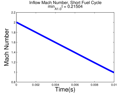
In other words, the minimizer $u_{in}^{*}$ is a straight line starting from $u_{0}$ and ending at $0.5u_{0}$, and equivalently, the minimizer $M_{in}^{*}$ is a straight line starting from $2$ and ending at $1$. Further, we obtain an upper bound for $\inf_{u_{in}\in\mathcal{A}}\mathcal{I}(u_{in})$:

$$\inf_{u_{in}\in\mathcal{A}}\mathcal{I}(u_{in})\leq\inf_{u_{in}\in\mathcal{B}}\mathcal{I}(u_{in})=\mathcal{I}(u_{in}^{*})=\frac{1}{2\sigma_{u}^{2}}\int_{0}^{T}\left(\frac{d}{dt}u_{in}^{*}(t)\right)^{2}dt=\frac{u_{0}^{2}}{8\sigma_{u}^{2}T}.$$ (15)

Thus we can conclude that when $\inf_{\tilde{u}_{in}\in\mathbf{A}}I(\tilde{u}_{in})$ is very close to this upper bound, the scramjet operates in a very stable region, because the probability of the unstart is as low as the theoretical limit.

Remark. One may analogously want to define $\mathbf{B}$ in the discrete sense. However, in general $\mathbf{B}$ is not necessarily a subset of $\mathbf{A}$ because in the definition of $\mathbf{A}$ (see (9)), what we check is if the Mach number in the second cell $M_{1}^{n}$ is less than $1$, but the inflow Mach number $M_{in}(n)=M_{0}^{n}\leq 1$ does not imply $M_{1}^{n}\leq 1$. In fact one often needs $M_{in}(n)=M_{0}^{n}\leq 1-\eta$ with a small positive $\eta$ to have $M_{1}^{n}\leq 1$. Therefore in the later numerical results, readers will find that the computed $\inf_{\tilde{u}_{in}\in\mathbf{A}}I(\tilde{u}_{in})$ in some cases will slightly higher than the continuum upper bound $u_{0}^{2}/(8\sigma_{u}^{2}T)$. Obviously this discrepancy will be reduced as we refine the discretization, and we still use this upper bound (15) as a reference value in our numerical results.

5.2 Impact of Fuel Cycles

The function of the fueling control is

$$f(t,x)=c\cdot\phi\cdot f(t)\cdot f(x),$$

where $c$ is a constant and $f(x)$ is a fixed spatial function. $\phi$ is the mixing ratio and $f(t)$ is the control of the fuel cycle:

$$f(t)=\begin{cases}1,&t\in[i\tau,i\tau+b],\quad i\in\mathbb{N},\\ 0,&\text{otherwise.}\end{cases}$$

In every fuel cycle of length $\tau$ seconds, the fuel is injected in the first $b$ seconds.

Two representative fueling profiles are used: $\phi_{S}=0.78$, $\tau_{S}=0.5$ms, $b_{S}=0.1$ms and $\phi_{L}=0.78$, $\tau_{L}=2$ms, $b_{L}=0.4$ms. These two profiles are extensively studied in [15]. Because $\phi_{S}=\phi_{L}$ and $b_{S}/\tau_{S}=b_{L}/\tau_{L}$, the two profiles generate roughly the same amount of thrust. However, the numerical experiments in [15] show that the first profile is more robust to prevent the engine from stalling. We observe the same qualitative behavior in the large deviation case.

Fig. 4: The Mach numbers in the scramjet engine when a constant inflow (Mach $2$) is used. The engine operates normally for both short and long fuel cycles.

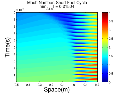
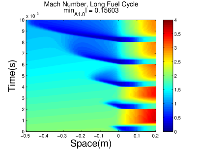
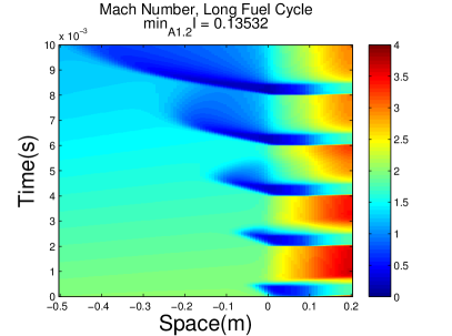
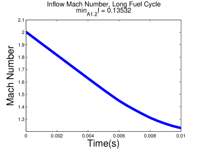
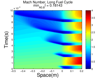
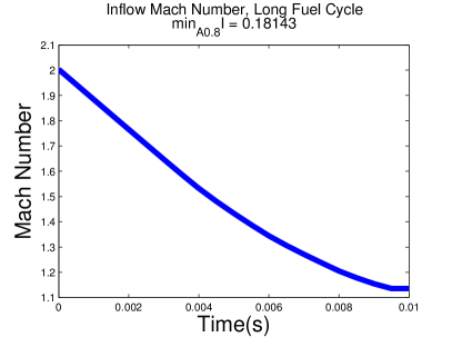
Fig. 5: The large deviation solutions of two different fuel cycles. The optimal $I$ of the short fuel cycle ($\phi_{S}$, $\tau_{S}$, $b_{S}$) is higher than that of the long fuel cycle ($\phi_{L}$, $\tau_{L}$, $b_{L}$). It means the short fuel cycle is a more stable strategy.

	Short Fuel Cycle	Long Fuel Cycle	$\mathcal{I}(u_{in}^{*})$
$\inf_{\tilde{u}_{in}\in\mathbf{A}}I(\tilde{u}_{in})$	$0.21504$	$0.15603$	$0.21125$

Table 1: The optimal values of the rate function for the short and long fuel cycles.

We can see in Figure 4 that with the constant inflow (Mach $2$), the engine operates operates normally for both fuel cycles. No subsonic flows reach the entrance of the isolator. In this section, Figure 4 will serve as the reference case representing the normal situation.

When the inflow perturbations are considered, we solve the large deviation problem $\inf_{\tilde{u}_{in}\in\mathbf{A}}I(\tilde{u}_{in})$. The solutions are plotted in Figure 5 (left). The optimal $I$ of the short fuel cycle ($0.21504$) is about $1/3$ higher than that of the long fuel cycle ($0.15603$). It means that when $\epsilon$ is small, the probability of the unstart with the short fuel cycle case is lower than that with the long fueling case. This observation is qualitatively consistent with the study in [15] by the Monte Carlo simulations.

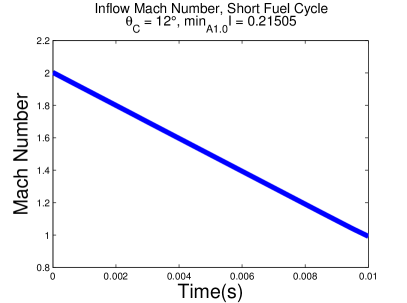
Figure 5 also tells us an interesting information: with the short fuel cycle, the minimizer for $\inf_{\tilde{u}_{in}\in\mathbf{A}}I(\tilde{u}_{in})$ is very close to a straight line starting from $2$ and ending at $1$, which is the minimizer $u_{in}^{*}(t)$ for the large deviation problem $\inf_{u_{in}\in\mathcal{B}}\mathcal{I}(u_{in})$ discussed in Section 5.1. In addition, its optimal value of the rate function ($0.21504$) is also close to the continuum upper bound ($0.21125$), which says that with the short fuel cycle, the scramjet has very strong resistance to the unstart.

5.3 Sensitivity to Constraints

We can slightly modify the constraint set $\mathbf{A}$ to see the sensitivity of the large deviation problem to the change of the constraint. More precisely, we define

$$\mathbf{A}_{0.8} =\{u_{in}=(u_{0}^{0},\ldots,u_{0}^{N}):~{}u_{0}^{0}=u_{0},~{}\min_{1\leq n\leq N}M_{1}^{n}\leq 0.8\},$$

$$\mathbf{A}_{1.2} =\{u_{in}=(u_{0}^{0},\ldots,u_{0}^{N}):~{}u_{0}^{0}=u_{0},~{}\min_{1\leq n\leq N}M_{1}^{n}\leq 1.2\},$$

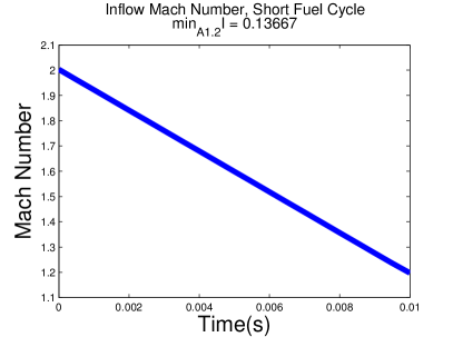
and let $\mathbf{A}_{1.0}:=\mathbf{A}$ in (9). It is reasonable to argue that $\mathbf{A}_{0.8}\subset\mathbf{A}_{1.0}\subset\mathbf{A}_{1.2}$ (by assuming that the Mach number is continuous in time.) Similarly, we can also define $\mathcal{B}_{0.8}$, $\mathcal{B}_{1.0}$ and $\mathcal{B}_{1.2}$ according to (13), and derive the continuum upper bounds by the formulas similar to (14) and (15) (see also Table 2).

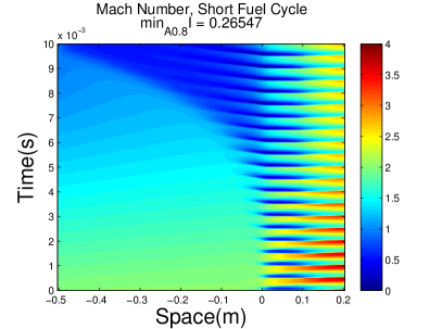
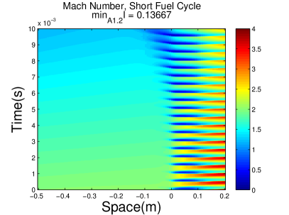
Fig. 6: The results of the large deviation problem by changing the constraint set $\mathbf{A}_{1.0}$ to $\mathbf{A}_{0.8}$ and $\mathbf{A}_{1.2}$ with the short fuel cycle.

Fig. 7: The results of the large deviation problem by changing the constraint set $\mathbf{A}_{1.0}$ to $\mathbf{A}_{0.8}$ and $\mathbf{A}_{1.2}$ with the long fuel cycle.

	Short Fuel Cycle	Long Fuel Cycle	$\mathcal{I}(u_{in}^{*})$
$\inf_{\tilde{u}_{in}\in\mathbf{A}_{0.8}}I(\tilde{u}_{in})$	$0.26547$	$0.18143$	$0.3042$
$\inf_{\tilde{u}_{in}\in\mathbf{A}_{1.0}}I(\tilde{u}_{in})$	$0.21504$	$0.15603$	$0.21125$
$\inf_{\tilde{u}_{in}\in\mathbf{A}_{1.2}}I(\tilde{u}_{in})$	$0.13667$	$0.13532$	$0.1352$

Table 2: The optimal rate functions over $\mathbf{A}_{0.8}$, $\mathbf{A}_{1.0}$ and $\mathbf{A}_{1.2}$. The values decrease with the looser constraints.

From Figure 6, with the short fuel cycle, when we consider the constraint set $\mathbf{A}_{1.2}$, the result is not too surprising: the most probable inflow Mach number is close to a straight line starting from Mach $2$ to Mach $1.2$, and the shock generated by the engine has no contribution. Indeed, the set $\mathbf{A}_{1.2}$ can be viewed as the case that the engine operates in a more normal condition, and in this case the effect of the engine is less than the effect in the case of $\mathbf{A}_{1.0}$ so the inflow Mach number is still the dominating effect. Nevertheless, when $\mathbf{A}_{0.8}$ is considered, the qualitative behavior changes. The most probable situation to have the Mach $0.8$ subsonic flow is because the shock generated by the engine reaches the entrance, and the most probable inflow Mach number is not a straight line. In fact, the end point of the most probable inflow Mach number is higher than $0.8$, which means that to in the sense of the large deviations, the scramjet does not need a inflow with Mach $0.8$ to trigger the event of $\mathbf{A}_{0.8}$.

Then we consider the case of the long fuel cycle. From Figure 6, we find that for the case of $\mathbf{A}_{1.2}$, the most probable inflow Mach number (upper right) is close to that of the short fuel cycle case (upper right in Figure 6), and their optimal values of the rate function are also close to the continuum upper bound (see Table 2). That means the shock generated by the engine is not the dominating effect in this case. For the case of $\mathbf{A}_{0.8}$, we can see that to have a subsonic flow of Mach $0.8$ at the entrance one just needs a supersonic inflow.

From Table 2, we can find that the optimal values of the rate function with the short fuel cycle are consistently higher than those with the long fuel cycle. This tells us that the strategy of the short fuel cycle is a more robust profile for the safety of the operation of the scramjet.

5.4 Impact of Engine Geometry

As Iaccarino et al. indicates in [5], the engine geometry greatly influences the safe operating region against the unstart. In theory, for a larger angle of combustor $\theta_{C}$, the engine can accommodate more heat and therefore the scramjet has a larger safe operation region. However, [5] also mentions that a excessively large $\theta_{C}$ will leads to the flow separation and cause the loss of thrust. The quasi-1D model cannot capture this phenomenon and therefore it can not be seen as well in our results. Readers may refer to [5] to see more details of the impact of $\theta_{C}$.

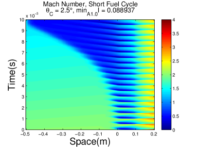
We also find the similar qualitative results in the large deviation sense. We change $\theta_{C}$ from $7.5^{\circ}$ (the typical setting in [5]) to two extreme values in [5], $\theta_{C}=2.5^{\circ}$ and $\theta_{C}=12^{\circ}$. In [5], the safe operation region of the scramjet is very small when $\theta_{C}=2.5^{\circ}$, and $\theta_{C}=12^{\circ}$ is considered as the largest angle of combustor without causing flow separation.

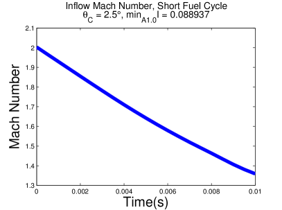
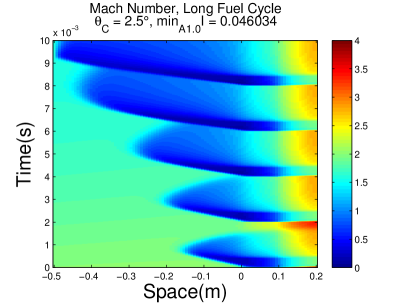
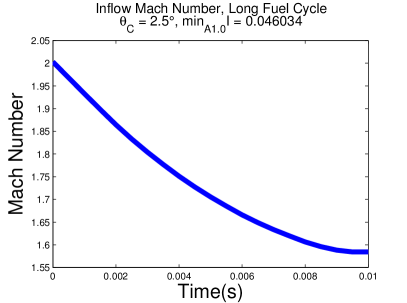
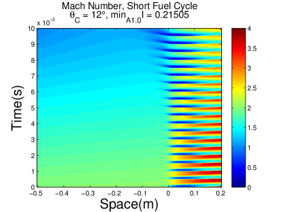
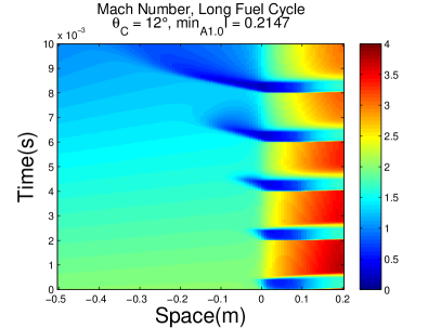
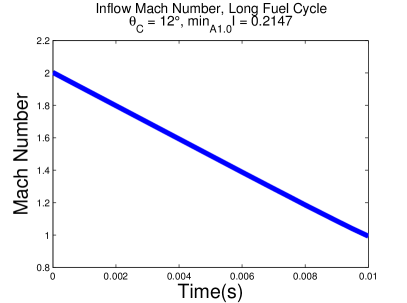
From Figure 8, we see that when $\theta_{C}=2.5^{\circ}$, the scramjet is not able to contain as much heat as before. Then the shock is build up and reaches the entrance. The optimal values of the rate function are very low so the unstart can happen very easily when $\theta_{C}=2.5^{\circ}$. On the other hand from Figure 9, when $\theta_{C}=12^{\circ}$, the optimal values of the rate function of both fueling profiles are close to the continuum upper bound and the minimizer are similar to $u_{in}^{*}$. This is because for a larger $\theta_{C}$, the engine has more space for the generated heat and the shock is not easy to move upstream.

Fig. 8: The large deviation solutions by changing $\theta_{E}$ from $7.5^{\circ}$ to $2.5^{\circ}$. The optimal values of the rate function are significantly decreased.

Fig. 9: The large deviation solutions by changing $\theta_{E}$ from $7.5^{\circ}$ to $12^{\circ}$. The optimal value of the high fuel cycle case is significantly increased. The optimal value of the short fuel cycle case is almost the same because the value already reaches the upper limit.

$\inf_{\tilde{u}_{in}\in\mathbf{A}_{1.0}}I(\tilde{u}_{in})$	Short Fuel Cycle	Long Fuel Cycle	$\mathcal{I}(u_{in}^{*})$
$\theta_{C}=2.5^{\circ}$	$0.088937$	$0.046034$	$0.21125$
$\theta_{C}=7.5^{\circ}$	$0.21504$	$0.15603$	$0.21125$
$\theta_{C}=12^{\circ}$	$0.21505$	$0.2147$	$0.21125$

Table 3: The optimal values of the rate function of different $\theta_{C}$. The higher $\theta_{C}$ have the higher optimal values

5.5 Resolutions of Large Deviation Solutions

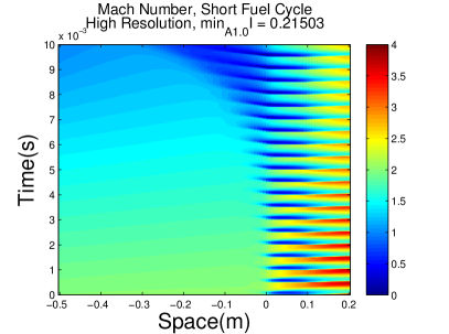
From the previous simulations, we are actually convinced that $\tilde{N}=20$ is the sufficient resolution of the large deviation solution due to the smoothness and the strong linearity of the solutions. Here we support our claim that $\tilde{N}=20$ is enough by doubling $\tilde{N}$ to $40$. If the results are very close, we can strongly believe our argument.

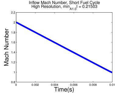
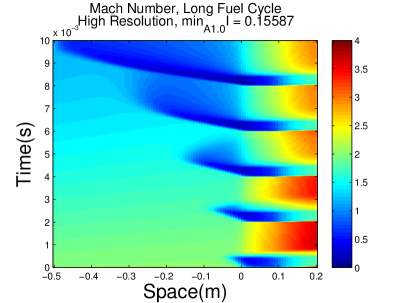
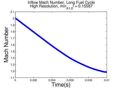
Fig. 10: The large deviation solutions with the high resolution. The settings are the same as those in Figure 5 but the solution resolution $\tilde{N}$ is doubled to $40$. The results are nearly the same and the relative differences between the optimal values of the rate function are less than $1\%$.

We use the same settings in Section 5.2, but let $\tilde{N}=40$ instead. From Figure 10, the optimal solutions are essentially the same, and the relative differences between the optimal values of the rate function are less than $1\%$.

$\inf_{\tilde{u}_{in}\in\mathbf{A}_{1.0}}I(\tilde{u}_{in})$	Short Fuel Cycle	Long Fuel Cycle	$\mathcal{I}(u_{in}^{*})$
$\tilde{N}=20$	$0.21504$	$0.15603$	$0.21125$
$\tilde{N}=40$	$0.21503$	$0.15587$	$0.21125$

Table 4: The optimal values of the rate function for different resolutions. The relative differences are less than $1\%$.

6 Monte Carlo Simulation with Importance Sampling

The large deviation results obtained in Section 5 is the exponential rate of decay of the probability, but are not the actual one. In this section we compute the probability of the unstart by using the Monte Carlo method.

6.1 Introduction to Importance Sampling

The most basic way to compute the probability of the unstart $\mathbb{P}(\mathbf{A})$ is to generate many independent sample paths $\{\tilde{u}^{j}_{in}\}_{j=1}^{J}$, where for each $j$, $\{\tilde{u}^{j}_{in}(n)\}_{n=0}^{N}$ satisfy (10) and (12). Then use the numerical PDE in Section 4.2.1 to determine if $\tilde{u}_{in}^{j}\in\mathbf{A}$. The basic Monte Carlo estimator is

$$\hat{P}^{MC}=\frac{1}{J}\sum_{j=1}^{J}1_{\mathbf{A}}(\tilde{u}_{in}^{j}).$$ (16)

Because $\mathbb{E}[\hat{P}^{MC}]=\mathbb{P}(\mathbf{A})$, $\hat{P}^{MC}$ is an unbiased estimator, which means that $\hat{P}^{MC}\to\mathbb{P}(\mathbf{A})$ almost surely as $J\to\infty$ by the law of large numbers. In addition, by the central limit theorem, the error bar of $\hat{P}^{MC}$ is proportional to its standard deviation

$$\mathbf{Std}(\hat{P}^{MC})=\frac{1}{\sqrt{J}}[\mathbb{P}(\mathbf{A})-\mathbb{P}^{2}(\mathbf{A})]^{1/2}.$$

In order to have a meaningful estimate, the order of the error bar should not exceed the order of the estimated probability. Namely,

$$\frac{\mathbf{Std}(\hat{P}^{MC})}{\mathbb{P}(\mathbf{A})}=\frac{1}{\sqrt{J}}\left(\frac{1}{\mathbb{P}(\mathbf{A})}-1\right)^{1/2}=\mathcal{O}(1).$$

The large deviation analysis tells us that as $\epsilon\ll 1$, $\mathbb{P}(\mathbf{A})$ decreases exponentially in $\epsilon$ so at the same time $J$ has to increase exponentially. The exponential growth of $J$ will eventually cause the basic Monte Carlo method computationally impossible.

To see what causes this computational difficulty, we note that the basic Monte Carlo estimator is simply the empirical frequency of $\tilde{u}_{in}\in\mathbf{A}$. When $\epsilon$ is small, only a very small fraction of the samples is meaningful (in $\mathbf{A}$), and most of the samples has no contribution to the estimation so resulting the inaccuracy of the estimator.

The well-established method to solve this issue is to use the importance sampling technique. The idea is that since most of the samples under the original measure $\mathbb{P}$ have no contribution, we use a different measure $\mathbb{Q}$ to sample $\tilde{u}_{in}^{j}$ so that there is a significant fraction of the samples contributing to the estimate. Since we bias the measure $\mathbb{P}$, a correction is needed to obtain an unbiased estimate. More precisely, we have

$$\mathbb{P}(\tilde{u}_{in}\in\mathbf{A})=\mathbb{E}_{\mathbb{P}}[1_{\mathbf{A}}(\tilde{u}_{in})]=\mathbb{E}_{\mathbb{Q}}[1_{\mathbf{A}}(\tilde{u}_{in})\frac{d\mathbb{P}}{d\mathbb{Q}}(\tilde{u}_{in})],$$

where $d\mathbb{P}/d\mathbb{Q}$ is the change of the measure. The importance sampling estimator is

$$\hat{P}^{IS}=\frac{1}{J}\sum_{j=1}^{J}1_{\mathbf{A}}(\tilde{u}_{in}^{j})\frac{d\mathbb{P}}{d\mathbb{Q}}(\tilde{u}_{in}^{j}),$$

where $\tilde{u}_{in}^{j}$ is sampled under $\mathbb{Q}$. Note that $\hat{P}^{IS}$ is unbiased as $\mathbb{E}[\hat{P}^{IS}]=\mathbb{P}(\tilde{u}_{in}\in\mathbf{A})$ and its standard deviation is

$$\mathbf{Std}(\hat{P}^{MC})=\frac{1}{\sqrt{J}}\mathbf{Std}(1_{\mathbf{A}}(\tilde{u}_{in})\frac{d\mathbb{P}}{d\mathbb{Q}}(\tilde{u}_{in})).$$

6.2 Large-Deviation-Based Importance Sampling

The main challenge of the importance sampling is how to choose $\mathbb{Q}$ (and therefore $d\mathbb{P}/d\mathbb{Q}$) to lower the standard deviation. A good choice may come from the solution of the large deviation problem $\inf_{\tilde{u}_{in}\in\mathbf{A}}I(\tilde{u}_{in})$. Assuming that the minimizer

$$\tilde{u}_{in}^{**}=\arg\inf_{\tilde{u}_{in}\in\mathbf{A}}I(\tilde{u}_{in}),$$

is unique, then for any open neighborhood $\mathbf{N}(\tilde{u}_{in}^{**})$ of $\tilde{u}_{in}^{**}$, we have the following asymptotic conditional probability:

$$\mathbb{P}(\tilde{u}_{in}\in\mathbf{N}(\tilde{u}_{in}^{**})|\tilde{u}_{in}\in\mathbf{A})=1-\mathbb{P}(\tilde{u}_{in}\in\mathbf{N}^{C}(\tilde{u}_{in}^{**})|\tilde{u}_{in}\in\mathbf{A})\\ =1-{\mathbb{P}(\mathbf{N}^{C}(\tilde{u}_{in}^{**})\cap\mathbf{A})}/{\mathbb{P}(\mathbf{A})}\overset{\epsilon\ll 1}{\approx}1-\frac{\exp(-\frac{1}{\epsilon^{2}}\inf_{\tilde{u}_{in}\in\mathbf{N}^{C}(\tilde{u}_{in}^{**})\cap\mathbf{A}}I(\tilde{u}_{in}))}{\exp(-\frac{1}{\epsilon^{2}}\inf_{\tilde{u}_{in}\in\mathbf{A}}I(\tilde{u}_{in}))}\overset{\epsilon\to 0}{\to}1.$$

In other words, the mass of the conditional probability is concentrated exponentially fast around the most probable path $\tilde{u}_{in}^{**}$. This observation motivates us to choose the measure $\mathbb{Q}$ so that the sampled $\tilde{u}_{in}^{j}$’s are centered around $\tilde{u}_{in}^{**}$.

Now we construct $\mathbb{Q}$ and $d\mathbb{P}/d\mathbb{Q}$ based on $\tilde{u}_{in}^{**}$. Recall that under $\mathbb{P}$, from (10) we have

$$\tilde{u}_{in}((n+1)m)=\tilde{u}_{in}(nm)+\epsilon\sigma_{u}\Delta\tilde{W}_{n+1}=u_{0}+\epsilon\sigma_{u}\sum_{l=0}^{n}\Delta\tilde{W}_{l+1},\quad n=0,\ldots,\tilde{N}-1,$$

We let $\mathbb{Q}$ such that under $\mathbb{Q}$, $\tilde{u}_{in}$ is a Gaussian random walk centered at $\tilde{u}_{in}^{**}$:

$$\tilde{u}_{in}((n+1)m)=\tilde{u}_{in}^{**}((n+1)m)+\epsilon\sigma_{u}\sum_{l=0}^{n}\Delta\hat{W}_{l+1},\quad n=0,\ldots,\tilde{N}-1,$$ (17)

where $\{\Delta\hat{W}_{n+1}\}_{n=0}^{\tilde{N}-1}$ are independent Gaussian random variables with mean zero and variance $m\Delta t$ under $\mathbb{Q}$. The intermediate variables are still determined by the linear interpolation (12). Note that $\{\tilde{u}_{in}(nm)\}_{n=1}^{\tilde{N}}$ are jointly Gaussian under both $\mathbb{P}$ and $\mathbb{Q}$ so the change of measure can be obtained explicitly:

$$\frac{d\mathbb{P}}{d\mathbb{Q}}(\tilde{u}_{in};\tilde{u}_{in}^{**})=\frac{\exp\left(-\frac{1}{\epsilon^{2}\sigma_{u}^{2}}(\tilde{\mathbf{u}}_{in}-\mathbf{u}_{0})^{\mathbf{T}}\mathbf{\Sigma}^{-1}(\tilde{\mathbf{u}}_{in}-\mathbf{u}_{0})\right)}{\exp\left(-\frac{1}{\epsilon^{2}\sigma_{u}^{2}}(\tilde{\mathbf{u}}_{in}-\tilde{\mathbf{u}}_{in}^{**})^{\mathbf{T}}\mathbf{\Sigma}^{-1}(\tilde{\mathbf{u}}_{in}-\tilde{\mathbf{u}}_{in}^{**})\right)},$$ (18)

where $\mathbf{u}_{0}$, $\tilde{\mathbf{u}}_{in}^{**}$ and $\tilde{\mathbf{u}}_{in}$ are $\tilde{N}$-dimensional column vectors:

$$\mathbf{u}_{0}=(u_{0},\ldots,u_{0}),\quad\tilde{\mathbf{u}}_{in}^{**}=(\tilde{u}_{in}^{**}(m),\ldots,\tilde{u}_{in}^{**}(\tilde{N}m)),\quad\tilde{\mathbf{u}}_{in}=(\tilde{u}_{in}(m),\ldots,\tilde{u}_{in}(\tilde{N}m)),$$

and $\mathbf{\Sigma}$ is the covariance matrix of $(\Delta\hat{W}_{1},\ldots,\Delta\hat{W}_{\tilde{N}})$ under $\mathbb{Q}$.

In summary, the large-deviation-based importance sampling is implemented as follows:

Algorithm 4.

1. Compute $\tilde{u}_{in}^{**}=\arg\inf_{\tilde{u}_{in}\in\mathbf{A}}I(\tilde{u}_{in})$ numerically by Algorithm 3.

2. Sample $J$ independent $\tilde{u}_{in}^{j}$ under $\mathbb{Q}$ by (17).

3. For each $j$, compute the change of measure $\frac{d\mathbb{P}}{d\mathbb{Q}}(\tilde{u}_{in}^{j};\tilde{u}_{in}^{**})$ in (18).

4. The large-deviation-based importance sampling estimator is

   $$\hat{P}^{IS}=\frac{1}{J}\sum_{j=1}^{J}1_{\mathbf{A}}(\tilde{u}_{in}^{j})\frac{d\mathbb{P}}{d\mathbb{Q}}(\tilde{u}_{in}^{j};\tilde{u}_{in}^{**}).$$

6.3 Simulation Results

Here we test the two estimators of the probability of the unstart: the basic Monte Carlo estimator $\hat{P}^{MC}$ and the large-deviation-based importance sampling estimator $\hat{P}^{IS}$. The event we test is $\mathbb{P}(\tilde{u}_{in}\in\mathbf{A})=\mathbb{P}(\tilde{u}_{in}\in\mathbf{A}_{1.0})$ (see (9) for the definition of $\mathbf{A}$) with the short and long fuel cycles (see Section 5.2). As the inflow condition is random, instead of the uniform time increment $\Delta t$, we use the adaptive time increment to ensure that the CFL condition is satisfied (see Appendix B for more details.)

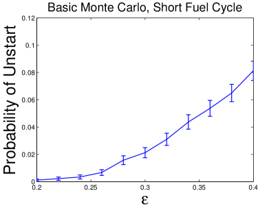
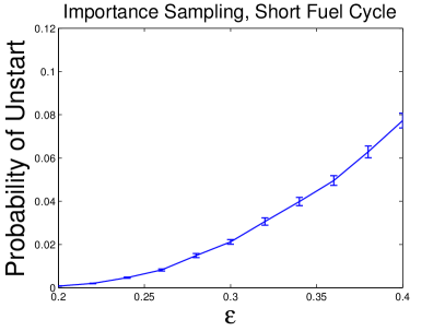
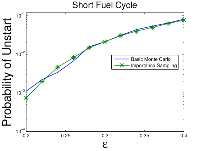
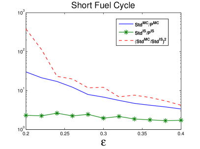
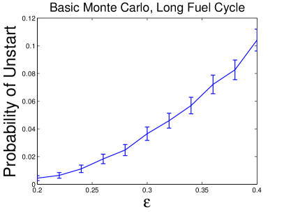
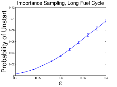
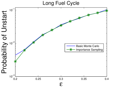
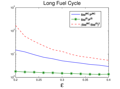
We let $J=10^{4}$ and test for $\epsilon=0.2,0.22,0.24,\ldots,0.4$, where $\mathbb{P}(\mathbf{A})=\mathcal{O}(10^{-1})$ for $\epsilon=0.4$ and $\mathbb{P}(\mathbf{A})=\mathcal{O}(10^{-3})$ for $\epsilon=0.2$. The (numerical) $99\%$ confidence interval and the (numerical) relative error are two quantities measuring the performance of the estimators. We define the numerical standard deviations as

$$(\mathbf{Std}^{MC}_{J})^{2}=\frac{1}{J-1}\sum_{j=1}^{J}(1_{\mathbf{A}}(\tilde{u}_{in}^{j})-\hat{P}^{MC})^{2},$$

$$(\mathbf{Std}^{IS}_{J})^{2}=\frac{1}{J-1}\sum_{j=1}^{J}(1_{\mathbf{A}}(\tilde{u}_{in}^{j})\frac{d\mathbb{P}}{d\mathbb{Q}}(\tilde{u}_{in}^{j};\tilde{u}_{in}^{**})-\hat{P}^{IS})^{2}.$$

Then the numerical $99\%$ confidence intervals are

$$[\hat{P}^{MC}-\frac{2.58}{\sqrt{J}}\mathbf{Std}^{MC}_{J},\hat{P}^{MC}+\frac{2.58}{\sqrt{J}}\mathbf{Std}^{MC}_{J}],\quad[\hat{P}^{IS}-\frac{2.58}{\sqrt{J}}\mathbf{Std}^{IS}_{J},\hat{P}^{IS}+\frac{2.58}{\sqrt{J}}\mathbf{Std}^{IS}_{J}],$$

and the numerical relative errors are $\mathbf{Std}^{MC}_{J}/\hat{P}^{MC}$ and $\mathbf{Std}^{IS}_{J}/\hat{P}^{IS}$.

Fig. 11: The basic Monte Carlo method and the importance sampling estimator for the probability of the unstart when the short fuel cycle is used (the top figures). The error bar are the $99\%$ confidence intervals. The bottom left figure is the plot of the estimated probabilities in the log scale. The bottom right figure is the plot of the relative errors $\mathbf{Std}^{MC}_{J}/\hat{P}^{MC}$ and $\mathbf{Std}^{IS}_{J}/\hat{P}^{IS}$, and the ratio of $\mathbf{Std}^{MC}_{J}$ to $\mathbf{Std}^{IS}_{J}$, which is the factor of the improvement of $\mathbf{Std}^{IS}_{J}$.

Fig. 12: The basic Monte Carlo method and the importance sampling estimator for the probability of the unstart when the long fuel cycle is used (the top figures). The error bar are the $99\%$ confidence intervals. The bottom left figure is the plot of the estimated probabilities in the log scale. The bottom right figure is the plot of the relative errors $\mathbf{Std}^{MC}_{J}/\hat{P}^{MC}$ and $\mathbf{Std}^{IS}_{J}/\hat{P}^{IS}$, and the ratio of $\mathbf{Std}^{MC}_{J}$ to $\mathbf{Std}^{IS}_{J}$, which is the factor of the improvement of $\mathbf{Std}^{IS}_{J}$.

From Figure 11 and 12 we see that $\hat{P}^{IS}$ has the more accurate estimates; the improvement of $\hat{P}^{MC}$ increases when the estimated probability decreases. We also note that although the importance sampling is intrinsically designed for the small $\epsilon$ situations, our simulations show that it also improves the non-small $\epsilon$ cases. Because the rare of convergence of $\hat{P}^{MC}$ and $\hat{P}^{IS}$ are $1/\sqrt{J}$, the improvement of the speed is the square of the ratio of the standard deviations $\mathbf{Std}^{MC}_{J}/\mathbf{Std}^{IS}_{J}$. Then we see that the improvement of the speed of $\hat{P}^{IS}$ ranges from a factor of $4.2$ ($\epsilon=0.4$) to a factor of $381.5$ ($\epsilon=0.2$) when the short is used, and from a factor of $5.4$ ($\epsilon=0.4$) to a factor of $170.3$ ($\epsilon=0.2$) if we use the long fuel cycle. Roughly speaking, the ratio of the improvement of is proportional to $1/\mathbb{P}(\mathbf{A})$.

7 Conclusion

In this paper, we use the large deviation principle to analyze the probability of unstart of a scramjet due to the random perturbation of the inflow. The numerical analysis is performed under various comparisons: the impact of the fueling schedules, the sensitivity to the constraint sets and the effect of the engine geometry, some of which are also confirmed and are consistent in the previous literature using the Monte Carlo method ([5, 15]); namely, the central analysis and the large deviation analysis have the high consistency on the region of operation. Further, the large deviation analysis gives a sharper information by providing the most probable inflow perturbation that causes unstart.

We also implement the large-deviation-based importance sampling to overcome the limitation of the basic Monte Carlo method. Our numerical results show that when the probability of unstart is small but still not negligible (for example, the order of $10^{-3}$ or even $10^{-4}$), the importance sampling is significantly better than the basic Monte Carlo. The theoretical ratio of the improvement can be up to the reciprocal of the estimated probability.

Appendix A List of Parameters

The listed parameters are the default values. We will mention the changes in the main text if different values are used.

Table 5: Table of Numerical Values

Variable	Name	Value	Units
State Variable
$\rho$	Density	-	$kg/m^{3}$
$u$	Flow Speed	-	$m/s$
$u_{in}$	Inflow Speed	-	$m/s$
$\rho u$	Mass Flow	-	$kg/m^{2}s$
$E$	Energy Density	-	$J/m^{3}$
$P$	Pressure	-	Pascals
$M$	Mach Number	-
$M_{in}$	Inflow Mach Number	-
$\gamma$	Ratio of Specific Heats	$1.4$
Geometry
$A_{0}$	Minimum Cross Sectional Area of Engine	$0.008$	$m^{2}$
$L_{I}$	Inlet Length	$0.5$	$m$
$L_{C}$	Combustor Length	$0.1$	$m$
$L_{E}$	Expansion Region Length	$0.1$	$m$
$\theta_{I}$	Angle of Inlet	$0.0$	Degrees
$\theta_{C}$	Angle of Combustor	$7.5$	Degrees
$\theta_{E}$	Angle of Expansion Region	$15.0$	Degrees
Fueling
$\phi$	Mixing Ratio	$0.78$
$f_{stoch}$	Stochiometirc Fuel/Air Ratio	$0.029$
$H_{prop}$	Fuel Heating Value	$1.2\times 10^{8}$	$J/Kg$
$\rho_{0}$	Free Stream Density - Taken as Inflow Density	$0.159$	$kg/m^{3}$
$u_{0}$	Free Stream Velocity - Take as Inflow Velocity	$1300.0$	$m/s$
$P_{0}$	Free Stream Pressure - Take as Inflow Pressure	$47842.0$	Pascals
$\tau_{S}$	Short Fuel Cycle Length	$0.5$	$ms$
$b_{S}$	Short Fuel Burst Length	$0.1$	$ms$
$\tau_{L}$	Long Fuel Cycle Length	$2$	$ms$
$b_{L}$	Long Fuel Burst Length	$0.4$	$ms$
Numerics
$T$	Terminal Time	$0.01$	$s$
$K$	Number of Cells	$100$
$N$	Number of Time Grids for Large Deviations	$10^{4}$
$\Delta t$	Time Increment of the Euler schemes (5) (8)	$10^{-6}$	$s$
$\tilde{N}$	Resolutions of $\tilde{u}_{in}$ in (10)	$20$
$\sigma_{u}$	Volatility of $u_{in}$	$10^{4}$	$m/s^{3/2}$
$\sigma_{M}$	Volatility of $M_{in}$	$96.9020$	$s^{-1/2}$

Appendix B Numerical PDE Methods of the Governing Equation

In this section, we describe the numerical method to solve the governing equation (1):

$$\begin{pmatrix}\rho\\ \rho u\\ E\\ \end{pmatrix}_{t}+\begin{pmatrix}\rho u\\ \rho u^{2}+P\\ (E+P)u\\ \end{pmatrix}_{x}=\frac{A^{\prime}(x)}{A(x)}\left(\begin{pmatrix}0\\ P\\ 0\\ \end{pmatrix}-\begin{pmatrix}\rho u\\ \rho u^{2}+P\\ (E+P)u\\ \end{pmatrix}\right)+\begin{pmatrix}0\\ 0\\ f(x,t)\\ \end{pmatrix}.$$

Given a spatial discretization: $-L_{I}=x_{0}<\cdots<x_{K}=L_{C}+L_{E}$, $X^{n}_{k}$ denotes the average of the quantity X over the cell $(x_{k},x_{k+1})$ at time $t_{n}$. We use the component-wise, first order local Lax-Friedrichs (LLF) scheme [13, Algoritm 4.4] to solve (1):

$$\begin{pmatrix}\rho_{k}^{n+1}\\ \rho_{k}^{n+1}u_{k}^{n+1}\\ E_{k}^{n+1}\\ \end{pmatrix}=\begin{pmatrix}\rho_{k}^{n}\\ \rho_{k}^{n}u_{k}^{n}\\ E_{k}^{n}\\ \end{pmatrix}-\frac{h}{\Delta x}(\mathcal{F}^{n}_{k+1/2}-\mathcal{F}^{n}_{k-1/2})\\ +h\frac{A^{\prime}(x_{k+1/2})}{A(x_{k+1/2})}\left(\begin{pmatrix}0\\ P_{k}^{n}\\ 0\\ \end{pmatrix}-\begin{pmatrix}\rho_{k}^{n}u_{k}^{n}\\ \rho_{k}^{n}(u_{k}^{n})^{2}+P_{k}^{n}\\ (E_{k}^{n}+P_{k}^{n})u_{k}^{n}\\ \end{pmatrix}\right)+h\begin{pmatrix}0\\ 0\\ f(x_{k+1/2},t_{n})\\ \end{pmatrix},$$ (19)

where $x_{k+1/2}=0.5(x_{k}+x_{k+1})$, $P_{k}^{n}=(\gamma-1)(E_{k}^{n}-\rho_{k}^{n}(u_{k}^{n})^{2}/2)$. $\mathcal{F}^{n}_{k\pm 1/2}$ are the numerical fluxes generated by the component-wise LLF method:

$$\mathcal{F}^{n}_{k+1/2} =\frac{1}{2}\left(\begin{pmatrix}\rho_{k+1}^{n}u_{k+1}^{n}\\ \rho_{k+1}^{n}(u_{k+1}^{n})^{2}+P_{k+1}^{n}\\ (E_{k+1}^{n}+P_{k+1}^{n})u_{k+1}^{n}\\ \end{pmatrix}+\begin{pmatrix}\rho_{k}^{n}u_{k}^{n}\\ \rho_{k}^{n}(u_{k}^{n})^{2}+P_{k}^{n}\\ (E_{k}^{n}+P_{k}^{n})u_{k}^{n}\\ \end{pmatrix}\right)$$

$$\quad-\frac{1}{2}\max\{|c_{k}^{n}+u_{k}^{n}|,|c_{k+1}^{n}+u_{k+1}^{n}|\}\left(\begin{pmatrix}\rho_{k+1}^{n}\\ \rho_{k+1}^{n}u_{k+1}^{n}\\ E_{k}^{n}\\ \end{pmatrix}-\begin{pmatrix}\rho_{k}^{n}\\ \rho_{k}^{n}u_{k}^{n}\\ E_{k}^{n}\\ \end{pmatrix}\right),$$

where $c_{k}^{n}=\sqrt{\gamma P_{k}^{n}/\rho_{k}^{n}}$ is the speed of sound. Because the component-wise scheme works well for the low-order methods (see [13]), we use it to reduce the computational cost.

For the inflow conditions, we let $\rho_{0}^{n}=\rho_{0}$ and $P_{0}^{n}=P_{0}$ for all $n$, and $u_{0}^{n}$ is governed by the stochastic inflow speed $u_{in}(n)$. For the outflow condition, the simple extrapolation is used: $(\rho_{K}^{n+1},u_{K}^{n+1},E_{K}^{n+1})=(\rho_{K-1}^{n},u_{K-1}^{n},E_{K-1}^{n})$.

The following strategy is used to find the suitable initial condition: we simulate the numerical PDE with $\rho(0,x)\equiv\rho(t,-L_{I})\equiv\rho_{0}$, $u(0,x)\equiv u(t,-L_{I})\equiv u_{0}$, $E(0,x)\equiv E(t,-L_{I})\equiv E_{0}$ and $f(t,x)\equiv 0$. Then with the aforementioned outflow extrapolation, the numerical solution obtained by this setting has the equilibrium state $(\rho^{e}(x),u^{e}(x),E^{e}(x))$ and use this state as the initial condition for the LDP.

In Section 4 and 5, the time increment $h$ is taken as the uniform constant $\Delta t$ in (8). This is because the uniform time grid results in a smoother constraint set $\mathbf{A}$ in (9), which increase the robustness of the numerical optimization $\inf_{\tilde{u}_{in}\in\mathbf{A}}I(\tilde{u}_{in})$. Because the inflow condition $\tilde{u}_{in}$ is a controlled variable, we can choose a sufficiently small $\Delta t$ so that the numerical scheme is stable when we solve $\inf_{\tilde{u}_{in}\in\mathbf{A}}I(\tilde{u}_{in})$. On the other hand, in Section 6, as the inflow condition is random and not controlled, we use the adaptive time increment:

$$h^{n}=0.8\times\frac{\Delta x}{\max_{k}|c_{k}^{n}+u_{k}^{n}|},$$

to satisfy the CFL condition and avoid the instabilities due to extraordinary inflow conditions.

References

• [1] O.A. Buchmann, Thermal-Structural Design Study of an Airframe-Integrated Scramjet, Tech. Report 3141, NASA, 1979.
• [2] T.R.A. Bussing and E.M. Murman, A One-Dimensional Unsteady Model of Dual Mode Scramjet Operation, in Proceedings of the 21st aerospace Sciences Meeting, AIAA, 1983.
• [3] A. Dembo and O. Zeitouni, Large deviations techniques and applications, vol. 38 of Stochastic Modelling and Applied Probability, Springer-Verlag, Berlin, 2010.
• [4] W. E, W. Ren, and E. Vanden-Eijnden, Minimum action method for the study of rare events, Comm. Pure Appl. Math., 57 (2004), pp. 637–656.
• [5] G. Iaccarino, R. Pecnik, J. Glimm, and D. Sharp, A QMU approach for characterizing the operability limits of air-breathing hypersonic vehicles, Reliability Engineering & System Safety, 96 (2011), pp. 1150 – 1160.
• [6] A. Jameson and J. Reuther, Control Theory Based Airfoil Design using Euler Equations, in Proceedings of AIAA/USAF/NASA/ISSMO Symposium on Multidisciplinary Analysis and Optimization, 1994.
• [7] J. Nocedal and S.J. Wright, Numerical optimization, Springer Series in Operations Research and Financial Engineering, Springer, New York, second ed., 2006.
• [8] S. O’Byrne, S.R. Doolan, and A.F.P. Houwing, Analysis of Transient Thermal Choking Processes in a Model Scramjet Engine, J. Prop. Power, 16 (2000), pp. 808–814.
• [9] B. Øksendal, Stochastic differential equations, Universitext, Springer-Verlag, Berlin, sixth ed., 2003.
• [10] D. Riggins, R. Tackett, and T. Taylor, Thermodynamic Analysis of Dual-Mode Scramjet Engine Operation and Performance, in Proceedings of the 14th AIAA/AHI Space Planes and Hypersonic Systems and Technologies Conference, AIAA, 2006.
• [11] T. Sato and S. Kaji, Study on Steady and Unsteady Unstart Phenomena due to Compound Choking and/or Fluctuations in Combustor of Scramjet Engines, in Proceedings of the Fourth International Aerospace Planes Conference, AIAA, 1992.
• [12] A.H. Shapiro, The Dynamics and Thermodynamics of Compressible Fluid Flow (Volume 1), Wiley, 1953.
• [13] C.-W. Shu, High order ENO and WENO schemes for computational fluid dynamics, in High-order methods for computational physics, vol. 9 of Lect. Notes Comput. Sci. Eng., Springer, Berlin, 1999, pp. 439–582.
• [14] Q. Wang, K. Duraisamy, J.J. Alonso, and G. Iaccarino, Risk Assessment of Scramjet Unstart Using Adjoint-Based Sampling Methods, AIAA Journal, 50 (2012), pp. 581–592.
• [15] N. West, G. Papanicolaou, P. Glynn, and G. Iaccarino, A Numerical Study of Filtering and Control for Scramjet Engine Flow, in 20th AIAA Computational Fluid Dynamics Conference, vol. 4, 2011, pp. 3010–3028.
• [16] X. Zhou, W. Ren, and W. E, Adaptive minimum action method for the study of rare events, The Journal of Chemical Physics, 128 (2008), p. 104111.