Numerical study of incommensurability of the spiral state on spin-1/2 spatially anisotropic triangular antiferromagnets using entanglement renormalization

Abstract

The ground state of an S=1/2 antiferromagnetic Heisenberg model on a spatially anisotropic triangular lattice, which is an effective model of Mott insulators on a triangular layer of organic charge transfer salts or Cs₂CuCl₄, is numerically studied. We apply a numerical variational method by using a tensor network with entanglement renormalization, which improves the capability of describing a quantum state. Magnetic ground states are identified for $0.7\leq J_{2}/J_{1}\leq 1$ in the thermodynamic limit, where $J_{1}$ and $J_{2}$ denote the inner-chain and inter-chain coupling constants, respectively. Except for the isotropic case ($J_{1}=J_{2}$), the magnetic structure is spiral with an incommensurate wave vector that is different from the classical one. The quantum fluctuation weakens the effective coupling between chains, but the magnetic order remains in the thermodynamic limit. In addition, the incommensurate wave number is in good agreement with that of the series expansion method.

I Introduction

The physics of Mott insulators has been attracting attention since the discovery of high-temperature superconductors. In the past decade, a number of new Mott insulator materials on a triangular layer have been found. For example, Cs₂CuCl₄Coldea et al. (2001) and organic charge transfer salts[Seeareviewarticle:][]Powell:2011ce, such as $\kappa$-(BEDT-TTF)₂ X and $\beta^{\prime}$-Z[Pd(dmit)₂]₂, have been extensively studied using experimental and theoretical approaches. At low temperatures in the Mott insulator phase, these materials show various equilibrium quantum states: an antiferromagnetic long-range ordered state, a valence bond crystal state, and a disordered state. In particular, the disordered behaviors in $\kappa$-(BEDT-TTF)₂ Cu₂ (CN)₃Shimizu et al. (2003); Yamashita et al. (2008, 2009), EtMe₃Sb[Pd(dmit)₂]₂Itou et al. (2008); Yamashita et al. (2010), and Cs₂CuCl₄Coldea et al. (2001) are of great interest.

Figure 1: (Color online) (a) Spatially anisotropic triangular lattice with two groups of interactions, denoted by dotted and solid links. $J_{1}$ and $J_{2}$ denote the coupling coefficients on each link. (b) The magnetic moment twist angle along the $J_{2}$ axis of the classical model (solid line) and the proposed phase diagrams of the quantum model (horizontal strips) on the spatially anisotropic triangular lattice. Here, SP and SL denote the spiral and spin-liquid phase, respectively.

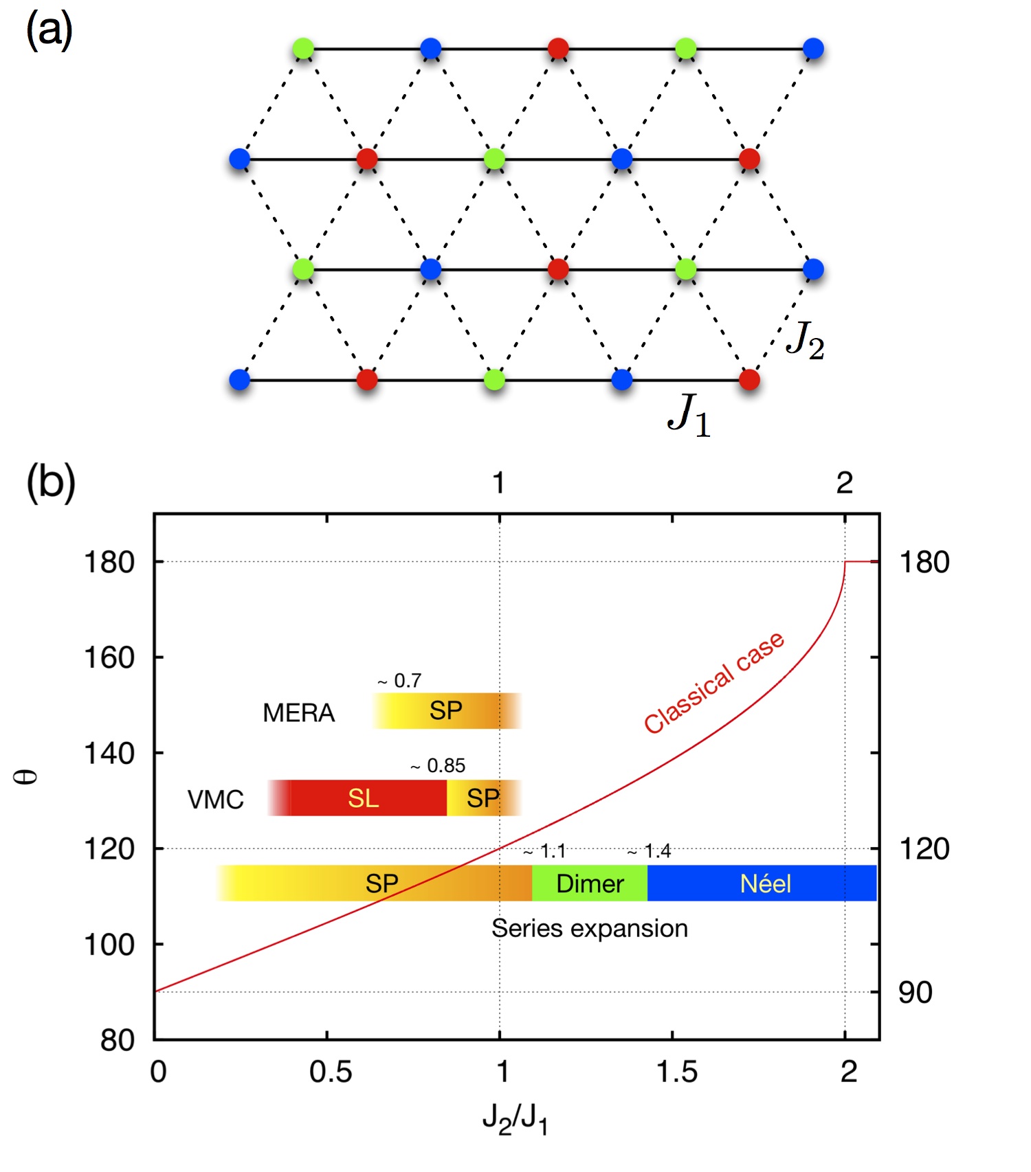
The simplest effective model of spin degrees in Mott insulators is the $S=1/2$ antiferromagnetic Heisenberg model on a triangular lattice. Since the triangular layer in a real material is distorted, we have two groups of Heisenberg interactionsPowell and McKenzie (2011). Figure 1(a) shows these two kinds of interactions as solid and dotted links. The Hamiltonian is written as

$$\mathcal{H}=J_{1}\sum_{\langle ij\rangle}\mathbf{S}_{i}\cdot\mathbf{S}_{j}+J_{2}\sum_{\langle\langle ij\rangle\rangle}\mathbf{S}_{i}\cdot\mathbf{S}_{j},$$ (1)

where $\langle ij\rangle$ and $\langle\langle ij\rangle\rangle$ denote pairs of sites on solid and dotted links in Fig. 1(a), respectively. The coupling coefficients $J_{1}$ and $J_{2}$ are positive. The ratio $J_{2}/J_{1}$ in real materials varies widely, from $\frac{1}{3}$ to $1$. For examplePowell and McKenzie (2011), $J_{2}/J_{1}$ for $\kappa$-(BEDT-TTF)₂ Cu₂ (CN)₃ was estimated to be close to 1, and that for Cs₂CuCl₄ was estimated to be about $\frac{1}{3}$.

Figure 2: (Color online) (a) Matrix product state for six sites: $T^{\mathrm{MPS}}_{s_{1},\cdots,s_{6}}$. (b) Tensor network with entanglement renormalization on a triangular lattice. Solid (red) lines represent tensor contractions for two connected tensor indices.

The model of Eq. (1) interpolates among independent chains ($J_{2}=0$), the fully frustrated triangular lattice ($J_{1}=J_{2}$), and the unfrustrated square lattice ($J_{1}=0$). Geometrical frustrations are present throughout the model, except at two special points($J_{1}=0$ and $J_{2}=0$). In the classical case, the ground state can be solved exactly: There are two long-range order phases at zero temperature [see Fig. 1(b)]: a Néel state on a square lattice for $J_{2}/J_{1}\geq 2$ and a spiral state with a smoothly changing wave number for $J_{2}/J_{1}\leq 2$. However, the phase diagram in the quantum model cannot be solved analytically. Thus, we have used various numerical or approximate methods. First, the ground state at the isotropic point ($J_{2}/J_{1}=1$) has been studied. For example, both exact diagonalization Bernu et al. (1994) and density matrix renormalization group (DMRG) calculations White and Chernyshev (2007) reveal a $120^{\circ}$ magnetic ordered ground state, whose wave number is equal to that in the classical model. Although quantum fluctuations reduce the magnetic moment magnitude, the $120^{\circ}$ magnetic ordered state was confirmed. However, the stability of the magnetic ordered state in the anisotropic region is controversial. Yunoki and SorellaYunoki and Sorella (2006) reported a disordered state for $J_{2}/J_{1}\lesssim 0.79$ by using a variational Monte Carlo (VMC) technique. In addition, Heidarian et al.Heidarian et al. (2009) reported the disappearance of magnetic long-range order at $J_{2}/J_{1}\sim 0.85$ by using another VMC technique. Weng et al. Weng et al. (2006) also reported a similar disordered state for $J_{2}/J_{1}\leq 0.78$ by using the DMRG method. Reuther and ThomaleReuther and Thomale (2011) reported a disordered state with collinear antiferromagnetic stripe fluctuations for $J_{2}/J_{1}<0.7\sim 0.9$ by using the pseudofermion functional renormalization group method. Thus, the disordered behavior in real materials may be captured by these states. However, some reports are contradictory, as shown in Fig. 1(b). Zheng et al. proposed a spiral phase for $0<J_{2}/J_{1}<1.11$ by using a series expansion methodZheng et al. (1999). Weichselbaum and White Weichselbaum and White (2011) also reported a long-rang magnetic correlation with an incommensurate wave vector in the whole region of $0<J_{2}/J_{1}\leq 1$ by using the DMRG method with different boundary conditions. The renormalization group analysesStarykh and Balents (2007); Ghamari et al. (2011) suggest a direct transition from spiral to collinear antiferromagnetic order at $J_{2}/J_{1}\lesssim 0.3$. Therefore, the stability of the spiral state in the quantum case is crucial for understanding the physical behavior of real materials.

In this study, a new numerical approach was used to calculate the ground state. Usually, quantum Monte Carlo (QMC) methods are powerful tools for two-dimensional quantum models, because they are unbiased. However, the weight of QMC samples can be negative in frustrated quantum magnets, leading to a cancellation in sign, and the accuracy of simulations fatally decreases (this is the so-called sign problem). Exact diagonalization can only be applied to small systems. Thus, a variational method has been chosen in this study. In particular, the key point of calculations in this study is the trial wave function. It is based on a tensor network with entanglement renormalization (ER)Vidal (2007). A tensor network is a theoretical tool in the field of quantum information to describe a quantum state. By modifying the network structure, we can freely design the structure of entanglements that mean quantum correlations in a quantum state. In general, the entanglement entropy of a subsystem is proportional to the area of the boundarySrednicki (1993). A tensor network with ER also obeys the area law of entanglement entropyBarthel et al. (2010). Though it only has a bias owing to the particular network structure used in the calculation, systematic error can be controlled, in principle, by increasing the dimensions of tensor indices. Therefore, the tensor network method is regarded as one of the most promising techniques for treating numerically unsolved problems such as the present one. Unfortunately, successful applications to quantum frustrated magnets in two dimensions are very few Evenbly and Vidal (2009a, 2010). In what follows, we demonstrate the usefulness of ER by applying it to the model of Eq. (1) to clarify the nature of its ground state.

By using the ER tensor networks shown in Fig. 2(b), the spiral state with incommensurate wave numbers for $0.7\leq J_{2}/J_{1}<1$ that overlaps with those of the disordered (spin liquid) phase reported in previous works Yunoki and Sorella (2006); Heidarian et al. (2009); Weng et al. (2006) was confirmed [see Fig. 1(b)]. In the numerical results, quantum fluctuations weaken the effective coupling between chains, but the long-range magnetic order remains in the thermodynamic limit. In addition, the incommensurate wave number is in good agreement with that obtained by the series expansion methodZheng et al. (1999). Since these two approaches are different, the results of this study provide strong evidence for the stable spiral phase.

The paper is organized as follows: In Sec. II, a tensor network with ER designed for triangular lattice models will be briefly introduced. In Sec. III, numerical calculations of the $S=1/2$ antiferromagnetic Heisenberg model on a spatially anisotropic triangular lattice will be reported. In Sec. IV, the results will be summarized.

II Tensor network with ER on a triangular lattice

II.1 Tensor network

Formally, the probability amplitudes of a wave function $|\psi\rangle$ can be regarded by a rank-$N$ tensor $T$ as $\langle s_{1},\cdots,s_{N}|\psi\rangle\equiv T_{s_{1},\cdots,s_{N}}$, where $N$ denotes the number of sites. However, we cannot treat a large-$N$-site system by using a tensor, because the number of elements in a rank-$N$ tensor exponentially increases. To avoid the exponential increase, we replace the original large-rank tensor by using a set of tensor contractions of small-rank tensors.

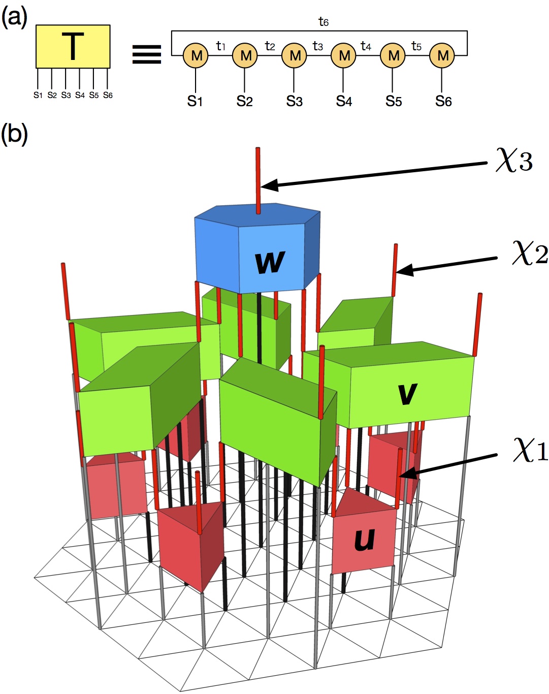
The tensor contractions can be drawn as a network. Thus, this type of wave function is called a tensor network wave function or, simply, a tensor network. The node of the network denotes a tensor, and the leg of the node denotes a tensor index. An edge connecting two legs represents a tensor contraction for the two corresponding indices. For example, Fig. 2(a) shows the tensor network for the probability amplitude as $T^{\mathrm{MPS}}_{s_{1},\cdots,s_{6}}\equiv\sum_{t_{1},\cdots,t_{6}}M_{t_{6},s_{1},t_{1}}\cdots M_{t_{5},s_{6},t_{6}}$. The one-dimensional tensor network is called a matrix product state (MPS). It is the general form of the wave function used in DMRG calculations.

II.2 ER on triangular lattices

Various types of tensor networks have been proposed for many-body quantum systems. The structure of the network affects entanglements in a tensor network state. For example, the MPS breaks the area law of entanglement entropy in more than two dimensions. Thus, in principle, it is not suitable for capturing the quantum state in two-dimensional quantum systems. To construct a tensor network for a triangular lattice model, we use a coarse-graining transformation removing short-range entanglements between coarse-grained regions. This is the ER method proposed by VidalVidal (2007). In particular, since the tensor network with ER obeys the area law of entanglement entropy, it can describe a quantum state with large entanglements in principle.

Figure 3: (Color online) Coarse-graining transformation for a triangular lattice model.

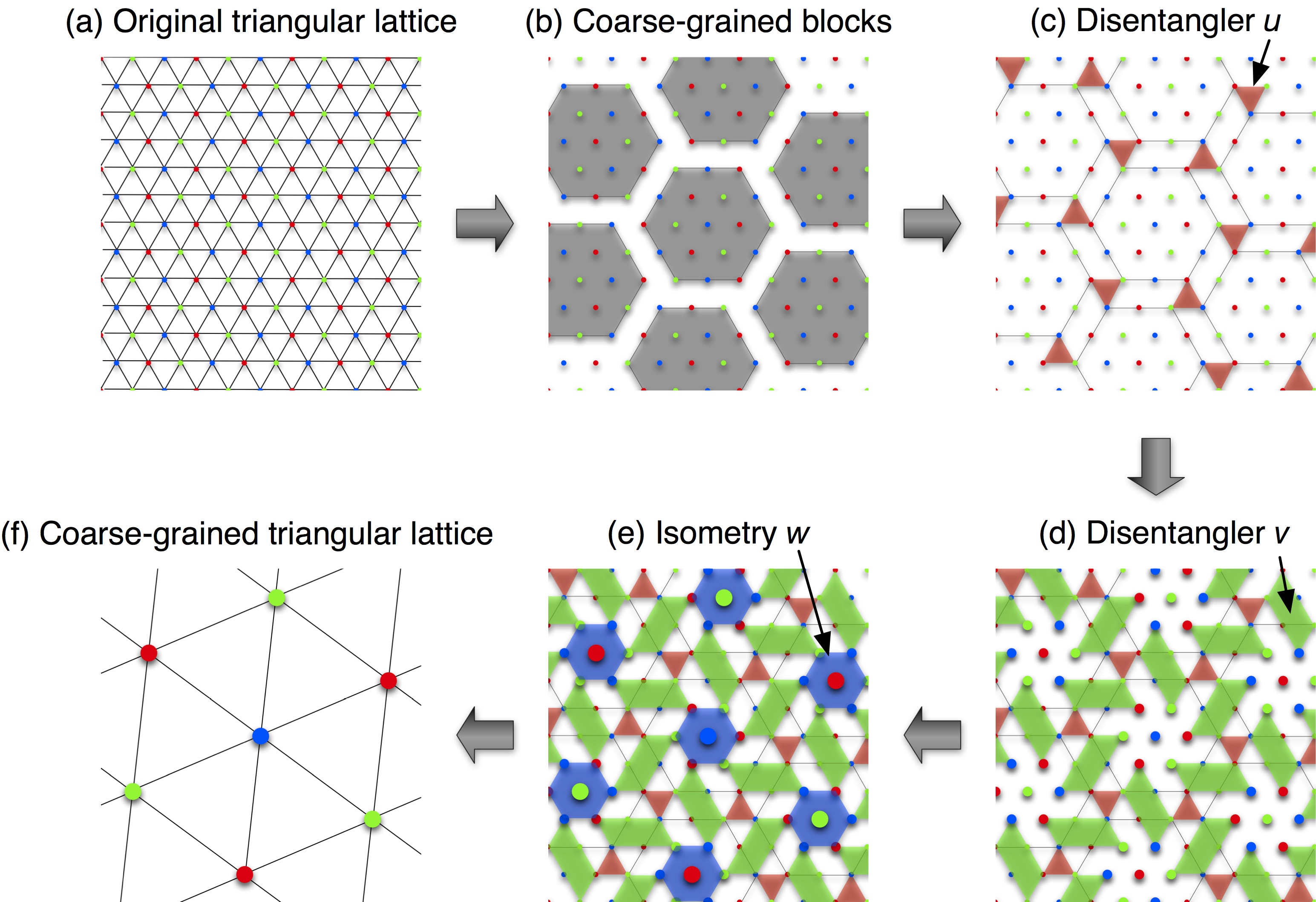
No systematic studies have been conducted on the optimal network structure. The empirical rule is that it should decrease the entanglement between coarse-grained regions as much as possible and, at the same time, keep the computational cost of tensor contractions reasonable. Figure 2(b) shows a suitable ER tensor network for triangular lattice models. It transforms a triangular lattice [Fig. 3(a)] to a coarse-grained one [Fig. 3(f)]. After the transformation, the number of sites decreases by a factor of $19$. The coarse-grained unit cell is the filled gray hexagon in Fig. 3(b). As shown in Fig. 2(b), the network consists of three sublayers. Each sublayer is occupied by a single type of tensor: $u$(red), $v$(green), and $w$(blue) from the bottom sublayer to the top sublayer, respectively, as shown in Fig. 2(b) and Fig. 3. Tensors $u$ and $v$ are called disentanglers, because their purpose is to decrease short-range entanglements between coarse-grained regions. The tensors have upper and lower legs. An upper leg in one sublayer is connected to the lower leg of a tensor in the higher sublayer. Disentangler $u$ has three lower legs and three upper ones. Disentangler $v$ has six lower legs and two upper ones. Tensor $w$ transforms seven sites to one site; this process is called isometry. In principle, the ER can be applied iteratively, and we usually finish the ERs corresponding to the top tensor on the last coarse-grained lattice, which is a simple isometry. In particular, the tensor network with multiple-level ERs is called a multiscale entanglement renormalization ansatz (MERA).

II.3 Computational costs of MERA

All tensors in MERA are isometric: $\sum_{k}(T^{i}_{k})^{*}T^{j}_{k}=\delta_{ij}$, where $T^{i}_{j}$ denotes the tensor’s element with index $i$ ($j$) of upper (lower) legs. Because of the isometric property, an expectation value of a local operator can be evaluated on a subnetwork that is finite and much smaller than the whole network, in most applications. This subnetwork is called a causal coneVidal (2007); Evenbly and Vidal (2009b); Giovannetti et al. (2009). Figure 4 shows a causal cone for the expectation value of an operator on a triangle plaquette of nearest neighbor sites. The number of tensors in a causal cone is proportional only to the logarithm of system size. Thus, the computational cost depends on the system size only weakly, compared to the exponential growth that is naturally expected. It only increases by a polynomial of dimensions of tensor indices.

Figure 4: (Color online) Causal cone for an expectation value of a local operator $A$ on a triangle plaquette of nearest neighbor sites $i$, $j$, and $k$: $\langle\psi|A(i,j,k)|\psi\rangle$. Here $|\psi\rangle$ is represented by the tensor network with an ER level defined in Fig. 2(b) and a top tensor that covers six sites as in Fig. 5. The local operator $A$ is drawn as a (yellow) tensor that has three upper and three lower legs. The upper and lower parts of the (yellow) tensor are subnetworks from $|\psi\rangle$ and $\langle\psi|$, respectively. We only draw tensor contractions between unpaired tensors as solid (red) lines. A tensor’s index without a solid (red) line in the upper part is always connected to that at the same position in the lower part. The width of a causal cone is defined by the number of solid (red) lines at the same height. The maximum width of this causal cone is six.

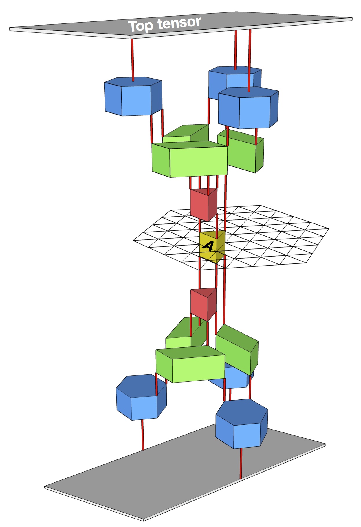
We assume that tensor legs at the same “height” have the same dimensions. Then the size of tensors in MERA can be specified by only an integer set as $(\chi_{1},\chi_{2},\chi_{3})$ in Fig. 2(b), where $\chi_{i}$ is the dimension of the upper index of tensors in the $i$th sublayer. The computational cost of the expectation value of operators on a triangle plaquette becomes a polynomial of these integers. As shown in Fig. 4, all tensors except the local operator drawn as (yellow) tensor $A$ are paired in a causal cone. We first calculate tensor contractions between paired tensors. Then, the causal cone is transformed to a tensor network that has a half height. Each tensor in the new tensor network is defined by paired tensors in the original network. If and only if an edge connects unpaired tensors, the edge remains in the new tensor network, as shown by the solid (red) lines in Fig. 4. Thus, the shape is similar to the upper part of the original one. The number of remaining lines at the same height in the new tensor network is called the width of the causal cone. Usually, we calculate this tensor network from the local operator drawn as (yellow) tensor $A$ in Fig. 4. The maximum number of indices of intermediate tensors is roughly double the maximum width of the causal cone. Thus, the memory size needed for calculating a causal cone rapidly increases with increasing dimensions of tensor indices. In fact, the maximum width of the causal cone in Fig. 4 is six. Since we use multithreaded subroutines for tensor contractions, the total memory size needed to calculate a causal cone is limited by the memory size of a computational node, which strictly limits the maximum dimensions of indices. In addition, the maximum polynomial degree for the computation of the causal cone is also larger than the double maximum width of causal cone. For example, the maximum polynomial degree in Fig. 4 is $14$. Since the Hamiltonian of Eq. (1) is written as the summation of local Hamiltonians on triangle plaquettes of nearest neighbor sites, the main part of the variational method can be decomposed into calculations of independent causal cones corresponding to local Hamiltonians. Thus, this part can be perfectly parallelized. Main calculations have been done using the facilities of the Supercomputer Center, Institute for Solid State Physics, University of Tokyo. In the largest case for the tensor network with two ER levels, 256 nodes were used.

III Numerical results obtained using a tensor network with ER

III.1 Isotropic triangular lattice

First, we calculate ground states of finite and infinite systems for $J_{1}=J_{2}$. The $120^{\circ}$ magnetic ordered state at the isotropic point has been confirmed by previous works (see Table III in Ref. Zheng et al., 2006). The purpose of this calculation is to test the variational wave function defined in the previous section and to see the behavior for an S=1/2 antiferromagnetic Heisenberg model on a triangular lattice.

III.1.1 Tensor network

The wave function consists of the single ER level in Fig. 3 with a top tensor. The top tensor covers six coarse-grained sites after the ER. Thus, this tensor network structure is applied to $N=6\times 19=114$ sites. Figure 5 shows the tensor network structure. Large solid circles denote the positions of coarse-grained sites. We put the top tensor on the parallelogram frame in Fig. 5. We apply this tensor network structure to both finite and infinite lattices. In this paper, we call the former the periodic boundary condition (PBC) scheme and the latter the infinite-size scheme, respectively.

In the PBC scheme, the total number of sites is just $6\times 19=114$. We set a skew PBC so that all parallelogram frames in Fig. 5 are the same. We notice that this PBC is consistent with a three-sublattice structure of a triangular lattice. In contrast, in the infinite-size scheme, we arrange the same tensor network structure, with $114$ sites per unit cell on an infinite lattice. Then the top layer is defined as the product state by top tensors. In addition, we assume that the tensors at the corresponding positions in all repeated units are the same. Thus, we can define a wave function by the finite set of tensors for the infinite lattice. This type of MERA is called a finite-correlation MERAEvenbly and Vidal (2009b), because reduced correlations become exactly zero for large distances. The distance limit for finite reduced correlations is roughly the size of the unit cell. The main difference between the two schemes lies in the causal cones. In the PBC scheme, all the causal cones are limited to one unit cell, because of the PBC. However, in the infinite-size scheme, some causal cones extend into multiple unit cells. Thus, the computational time for the infinite-size scheme may be longer than that for the PBC scheme.

Figure 5: (Color online) Tensor network structure with a single ER level and a top tensor for six coarse-grained sites. Big solid circles denote positions of sites on the coarse-grained lattice. The top tensor is put on the parallelogram frame. All parallelogram frames are the same by a skew periodic arrangement.

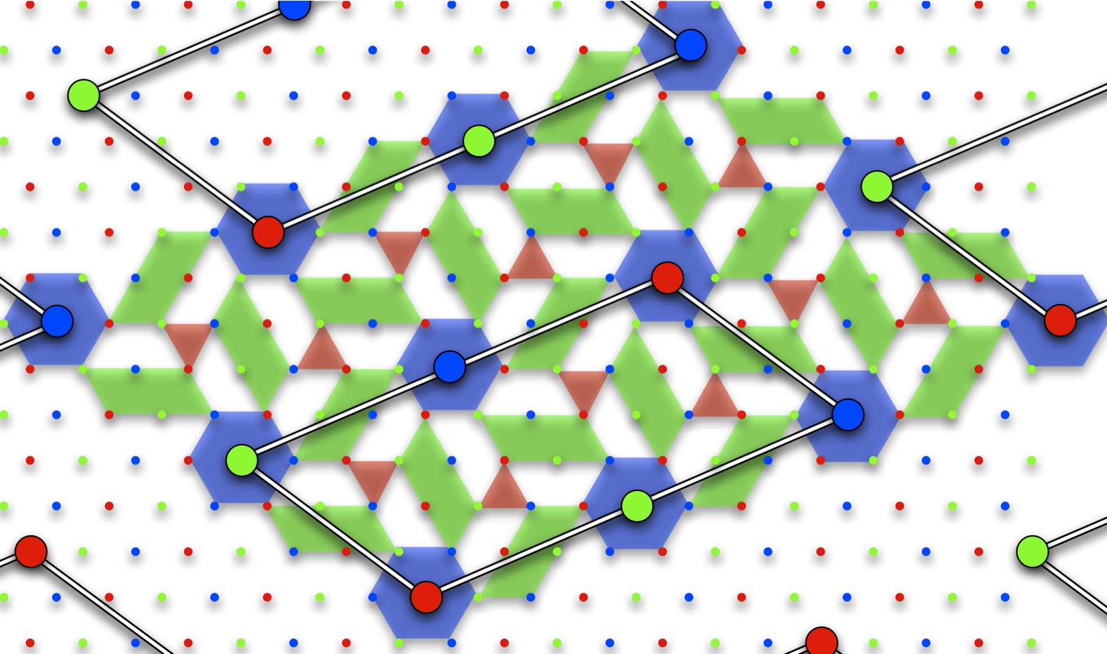
We assume that all tensors are independent within the unit cell to have more variational freedom with less bias. They were optimized to minimize the total energy of the tensor network states. The tensors are iteratively updated by the singular value decomposition method Evenbly and Vidal (2009b). Although this minimization problem may have some local minimum states, stable results starting from random initial tensors were obtained.

III.1.2 Energy

The ER tensor network for this study has the spatial structure shown in Fig. 3. As we mentioned above, if we use the finite dimension of the tensor index, the network-structure bias may cause a significant systematic error. To check whether or not this is the case, we try several sets of dimensions of tensor indices. Figure 6 shows local energies on finite and infinite lattices for various tensor sizes. The value of the local energy on a triangle plaquette defined by nearest neighbor sites $i$, $j$, and $k$, $\mathbf{S}_{i}\cdot\mathbf{S}_{j}+\mathbf{S}_{j}\cdot\mathbf{S}_{k}+\mathbf{S}_{k}\cdot\mathbf{S}_{i}$, is shown on a color scale. In the $120^{\circ}$ state, which we believe is the ground state in the present case, the local energy is homogeneous. Therefore, we expect that the whole system should be uniformly colored if the error of the calculation is sufficiently small. Figures 6(a) and 6(c) show the results of small tensor size, $(\chi_{1},\chi_{2},\chi_{3})=(2,2,2)$, for PBC and infinite-size schemes of $N=114$, respectively. There are clear spatial patterns resulting from the structure of ER in both cases. Increasing the tensor size should improve the quality of the tensor network states. In fact, as shown in Figs. 6(b) and 6(d), the patterns are clearly more homogeneous than for small tensors. We notice that the patterns in the infinite-size scheme are quite similar to those of the PBC scheme. Thus the assumption of direct product states for infinite systems does not affect the spatial pattern of local energies in the tensor network states.

Figure 6: (color online) Local energies on the triangular plaquettes. The value of the local energy on a triangle plaquette defined by nearest neighbor sites $i$, $j$ and $k$, $\mathbf{S}_{i}\cdot\mathbf{S}_{j}+\mathbf{S}_{j}\cdot\mathbf{S}_{k}+\mathbf{S}_{k}\cdot\mathbf{S}_{i}$, is shown by the color scale. The bottom bar shows the correspondence between the value of local energy and color. Results of the PBC scheme are shown in (a) and (b). Those of the infinite-size scheme are shown in (c) and (d). The size of tensors in (a) and (c) is $(\chi_{1},\chi_{2},\chi_{3})=(2,2,2)$. In (b) and (d), $(\chi_{1},\chi_{2},\chi_{3})=(2,8,8)$.

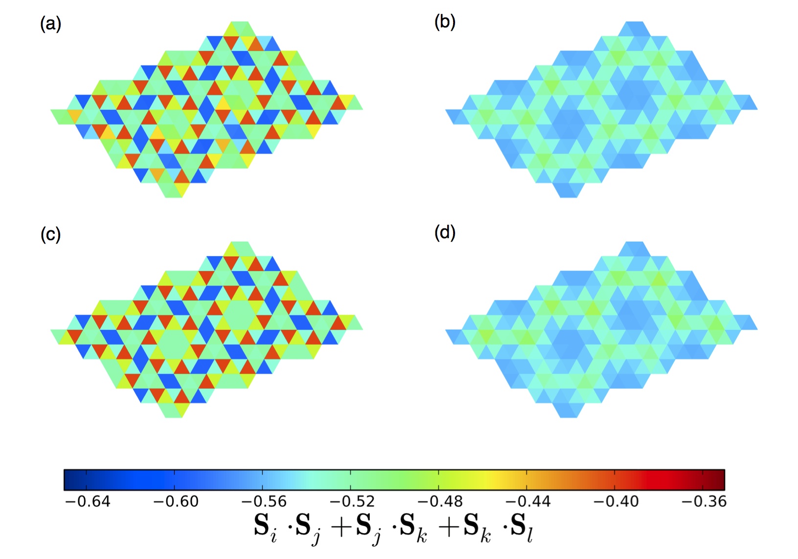
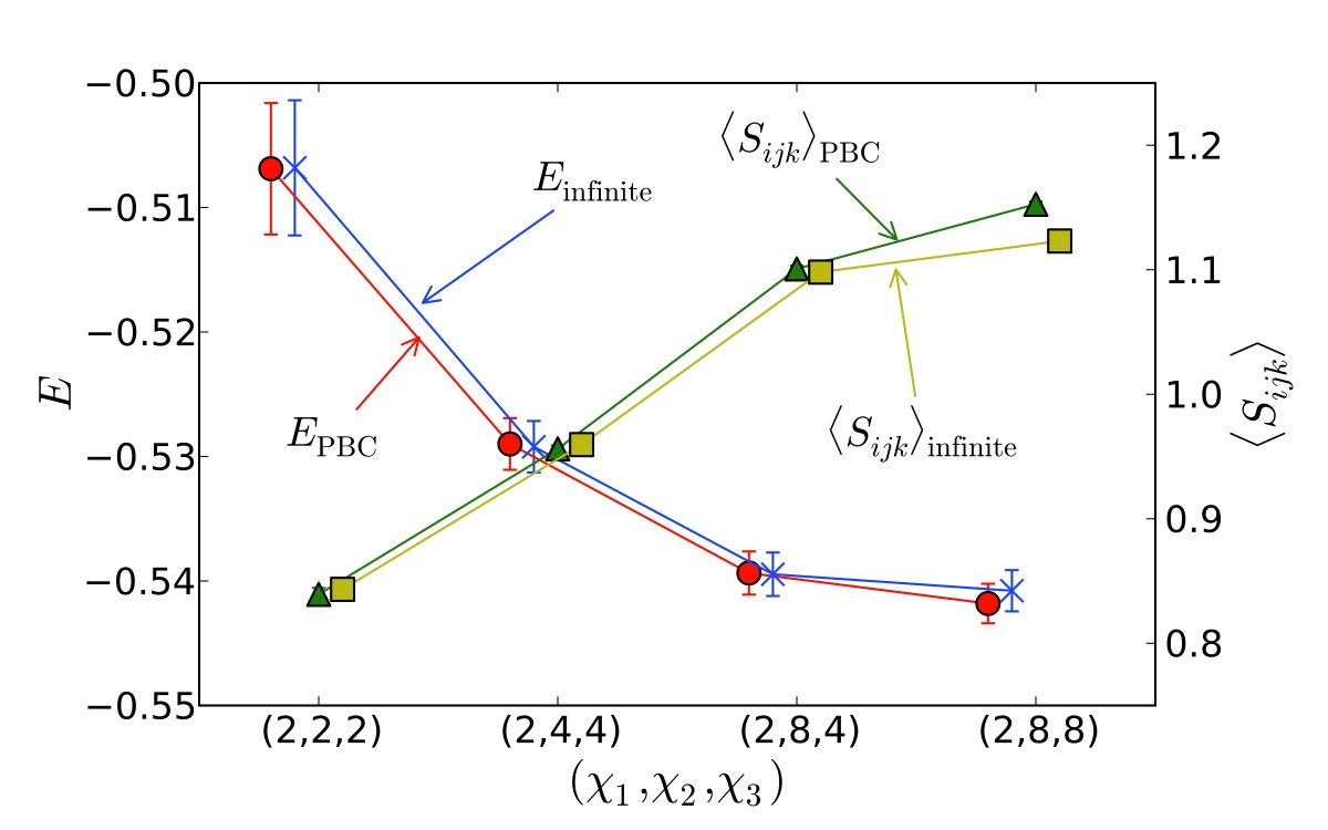
Figure 7 shows the energy per site, $E$, for the tensor sets $(\chi_{1},\chi_{2},\chi_{3})=(2,2,2),\ (2,4,4),\ (2,8,4),$ and $(2,8,8)$ for both PBC and infinite-size schemes. When the tensor size increases, the energy of tensor networks is indeed improved. The lowest energy per site at $(2,8,8)$ is $E_{\rm PBC}(N=114)=-0.54181$ and $E_{\rm inf}(N=114)=-0.54086$. These values compare well with results obtained from other methods (see Table III in Ref. Zheng et al., 2006). In particular, the result of a Green’s function quantum Monte Carlo (GFQMC) calculation with stochastic reconfiguration (SR)Capriotti et al. (1999) is $E(N=144)=-0.5472(2)$. Direct comparison may be difficult, because the skew boundary in this study is not equal to the periodic one used by the authors of Ref. Capriotti et al., 1999 and the lattice ($N=114$) in this study is smaller than their lattice ($N=144$). However, the result of this study is close to their result (:$1\%$ lower than its). The result for the infinite-size scheme also agrees well with previous estimates for the thermodynamic limit. In particular, it compares favorably to that of a series expansionZheng et al. (2006), $E=-0.5502(4)$, and to that from a GFQMC with SR calculationCapriotti et al. (1999), $-0.5458(1)$, in the thermodynamic limit.

Figure 7: (Color online) Energy per site, $E$, and the average of entanglement entropies on triangle plaquettes, $\langle S_{ijk}\rangle$, for PBC and infinite-size schemes ($N=114$). Circles (red) and crosses (blue) denote $E$ for PBC and infinite-size schemes, respectively. Triangles (green) and squares (yellow) denote $\langle S_{ijk}\rangle$ for PBC and infinite-size schemes, respectively. The error bar of $E$ shows the deviation of local energies on triangular plaquettes.

III.1.3 Entanglement entropy

Figure 8: (color online) Entanglement entropy of triangular plaquettes defined by nearest neighbor sites $i$, $j$, and $k$ in ER tensor network states. The bottom bar shows the correspondence between the value of entanglement entropy $S_{ijk}$ and color. The schemes and tensor sizes from (a) to (d) are equal to those from (a) to (d) in Fig. 6, respectively.

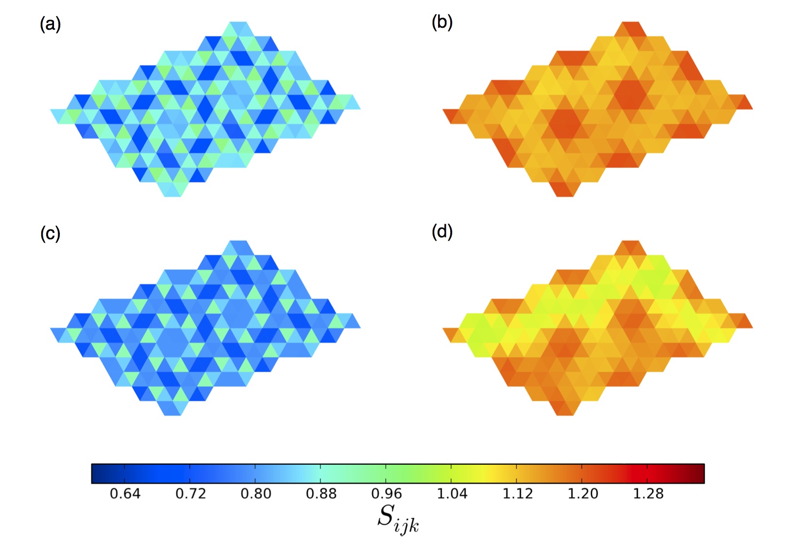
Entanglement entropy measures the quantum correlation between a considered region and another region. Figure 8 shows the entanglement entropy of a triangular plaquette on a color scale. It is defined as

$$S_{ijk}\equiv-{\rm Tr}[\rho_{ijk}\ln\rho_{ijk}],$$ (2)

where $\rho_{ijk}$ is the reduced density matrix of sites $i$, $j$, and $k$ on a triangle plaquette. There is clear spatial inhomogeneity owing to the network-structure bias, as is also seen in the local energy. The entanglement entropies on the boundary of coarse-grained regions are lower. When the tensor size increases, the average value of entanglement entropies also increases, as shown in Fig. 7. However, as shown in Figs. 8(b) and 8(d), the spatial patterns of entanglement entropies are different. In the infinite-size scheme, the boundary of unit cell has weak entanglement entropies. The reason for this is that the top layer is a direct product state. Although the assumption of a direct product state does not affect the spatial pattern of local energies, that of entanglement entropy is more sensitive. Thus, the entanglement entropy may be useful for checking wave function quality in other cases.

III.1.4 Magnetization

Figure 9: (color online) Averages on-site magnetizations on triangular plaquettes. The bottom bar shows the correspondence between the value of average on-site magnetizations and color. The schemes and tensor sizes from (a) to (d) are equal to those from (a) to (d) in Fig. 6, respectively.

Figure 10: (Color online) Average on-site magnetizations and average angles between magnetic moments of nearest neighbor sites. These results are obtained by the infinite-size scheme ($N=114$). The horizontal axis denotes energy per site. The left and right vertical axes denote the average on-site magnetizations on all sites and at the centers of ER, $M$ and $M_{c}$, and the average angle between magnetic moments of nearest neighbor sites, $\theta$, respectively. Circles (red), squares (green), and triangles (blue) denote points $(E_{\rm inf}(N=114),M)$, $(E_{\rm inf}(N=114),M_{c})$, and $(E_{\rm inf}(N=114),\theta)$, respectively. Solid (red), dotted (green), and dashed (blue) lines are fitting curves for them, respectively. The triplet $(\chi_{1},\chi_{2},\chi_{3})$ denotes the tensor size.

The magnetization on a site $i$ is defined as

$$M_{i}\equiv\sqrt{\langle\mathbf{S}_{i}\rangle\cdot\langle\mathbf{S}_{i}\rangle},$$ (3)

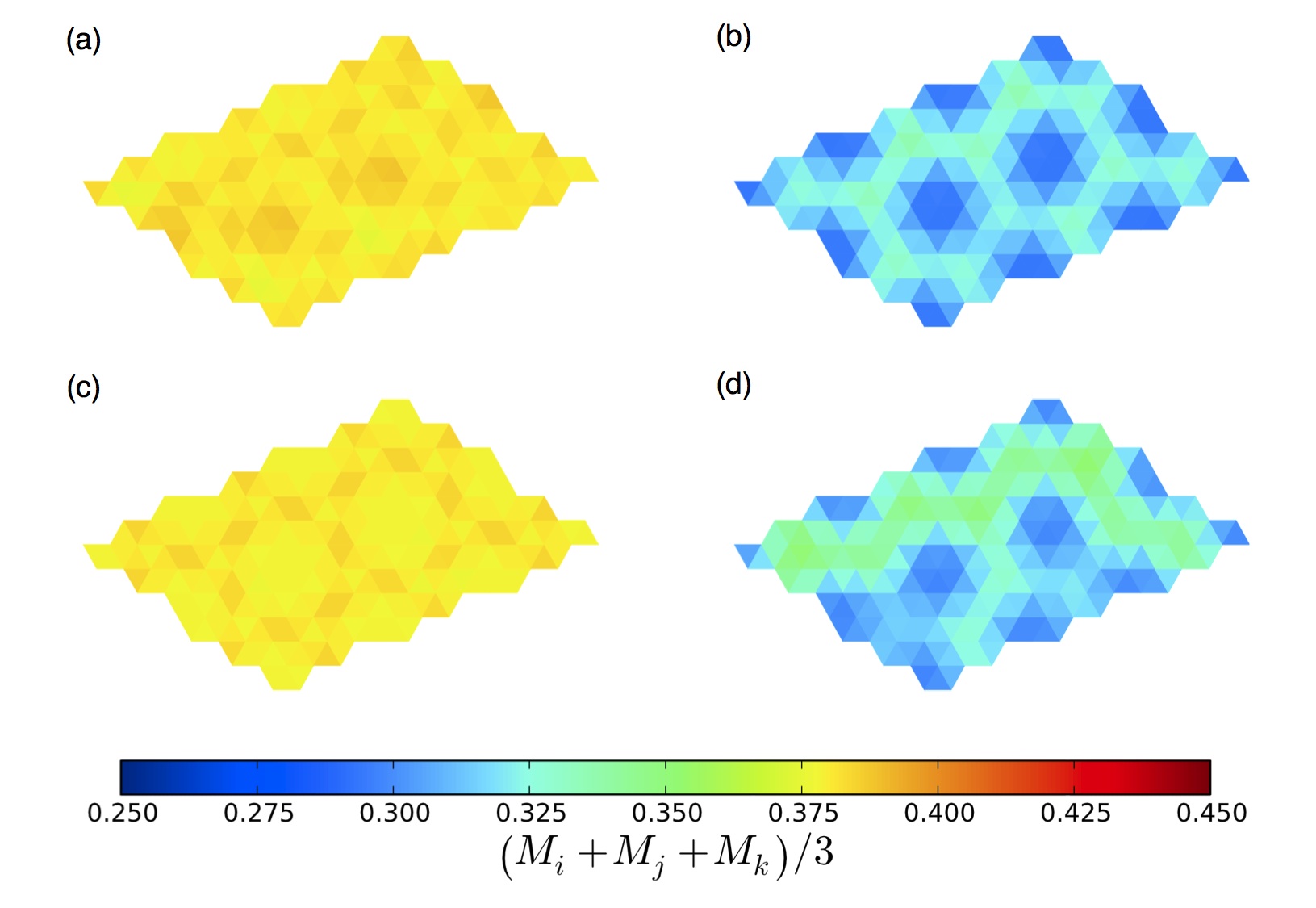
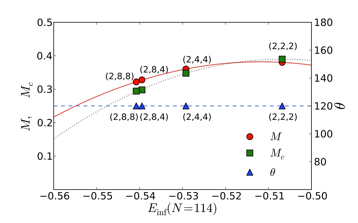
where $\langle\cdot\rangle$ denotes the expectation value of the operator by a variational wave function. Figure 9 shows the average on-site magnetizations on a triangular plaquette. They depend on the tensor size, and they show spatial patterns that depend on the structure of the ER tensor network. In addition, as seen in the case of entanglement entropy, the direct-product nature on the top layer also gives rise to spatial inhomogeneity. To make the extrapolation possible, we plot estimates of the magnetization as a function of the corresponding estimates of energy. Figure 10 shows the average on-site magnetizations obtained by using the infinite-size scheme ($N=114$), $M$, for various tensor sizes. The vertical and horizontal axes denote $M$ and $E_{\rm inf}(N=114)$, respectively. The dependence of $M$ on the tensor size is high. While the magnetization for the largest tensor size is $0.322(2)$ [see the left-most (red) circle], we cannot simply extrapolate it. The solid (red) curve is fitted to points of $M$. If we trust the $M-E$ curve, and if we take an estimate of the energy $E\in(0.54,0.55)$ upon which various previous works agree, we can conclude that $M\in(0.275,0.327)$. However, the result of this study is clearly larger than previous estimates: $M=0.205(15)$ from DMRG calculationsWhite and Chernyshev (2007), $M=0.205(10)$ by GFQMC with SR calculationsCapriotti et al. (1999), and $M=0.19(2)$ by series expansionZheng et al. (2006). As shown in Fig. 9, the reason for this discrepancy may be the spatial inhomogeneity caused by disentangling with small tensors. In DMRG calculations, to suppress the effect of the boundary condition as pinning the field on boundary sites, only on-site magnetization at the center of the system was usedWhite and Chernyshev (2007). To suppress the effect of incomplete disentangling, we also use on-site magnetization only at centers of ER, $M_{c}$. Figure 10 plots the average on-site magnetizations at six centers of ER. If we assume the same condition for extrapolating $M$, we can conclude that $M_{c}\in(0.232,0.298)$. This value is significantly close to other estimations. It is probable that the estimate of the magnetization in this study is an overestimate owing to the intrinsic bias of the tensor network that generally favors states with less entanglement entropy. From this view point, estimating the magnetization at a position with larger ER may be more appropriate than simply taking the spatial average.

However, the angle between magnetic moments of nearest neighbor sites converges, even when the tensor size is small. Figure 10 shows the average angle between magnetic moments of nearest neighbor sites, $\theta$, for various tensor sizes. The angle between magnetic moments of sites $i$ and $j$ is defined as

$$\theta_{ij}\equiv\left(\frac{180^{\circ}}{\pi}\right)\arccos\left[\frac{\langle\mathbf{S}_{i}\rangle\cdot\langle\mathbf{S}_{j}\rangle}{M_{i}M_{j}}\right].$$ (4)

All values in Fig. 10 are $120.0(4)$. Therefore, the ground state of an S=1/2 antiferromagnetic Heisenberg model on an isotropic triangular lattice is a magnetic ordered state with $120^{\circ}$ structure. This result is consistent with results from many previous works (see Table III in Ref. Zheng et al., 2006).

III.2 Spatially anisotropic triangular lattice of $J_{2}\leq J_{1}$

Results of variational calculations for a spatially anisotropic triangular lattice will be reported. We only consider the case of $J_{2}\leq J_{1}$ in this study. Our main interest lies in the robustness of the spiral magnetic ordered state.

III.2.1 Tensor network

As in the classical model, since the wave vector of a spiral magnetic ordered state may be incommensurate, we have to be careful about the periodicity in the variational wave function. Because of the finiteness of the unit cell in the tensor network, the wave vector of the magnetic ordered state is restricted. This restriction may cause a strong bias in variational calculations, in contrast to the case of an isotropic triangular lattice, where the unit cell of the ER tensor network in this study is perfectly consistent with the three-sublattice ordered state.

To weaken the finite-size effect of the unit cell, the number of ER levels was increased. In the MERA tensor network, the size of the unit cell increases exponentially by the number of ER levels. A tensor network with two ER levels has been used. The unit cell covers $6\times 19\times 19=2166$ sites. In addition, we make all tensors in the unit cell independent. Thus, the wave vector restriction is relaxed compared to the tensor network with a single ER level. In detail, the reciprocal vector is written as

$$\mathbf{k}=\frac{l}{4332}\left(\begin{array}[]{c}33\\ 63\sqrt{3}\end{array}\right)+\frac{m}{4332}\left(\begin{array}[]{c}41\\ 11\sqrt{3}\end{array}\right),$$ (5)

where the number of independent sets, $(l,m)$, is 2166, because of the skew periodic arrangement of the unit cell in Fig. 5. This number is $19$ times that for the single ER case. Although the number of independent causal cones also becomes $19$ times greater than before, parallel computing was used to calculate them. However, because of the memory size limit in a computational node, the calculations are limited to a tensor of size $\vec{\chi}=(\chi_{1},\chi_{2},\chi_{3},\chi_{4},\chi_{5},\chi_{6})=(2,8,4,4,8,4)$.

III.2.2 Energy and quantum mutual information

The variational calculations by PBC and infinite-size schemes with two ER levels ($N=2166$) have been performed.

As we see in the case of the single ER level, there is spatial inhomogeneity resulting from the structure bias of ER in both cases. By increasing the tensor size, we can systematically improve the quality of the tensor network states as before. In the single-ER calculation, as shown in Fig. 8(d), a weak entanglement region between unit cells exists in the infinite-size scheme. However, it disappears in the infinite-size scheme with two ER levels. Because of the large unit cell obtained by the two ER levels, the finite-size effect of the unit cell for entanglement entropy is sufficiently removed. In the following, the results of an infinite lattice will be mainly reported, which directly corresponds to the thermodynamic limit.

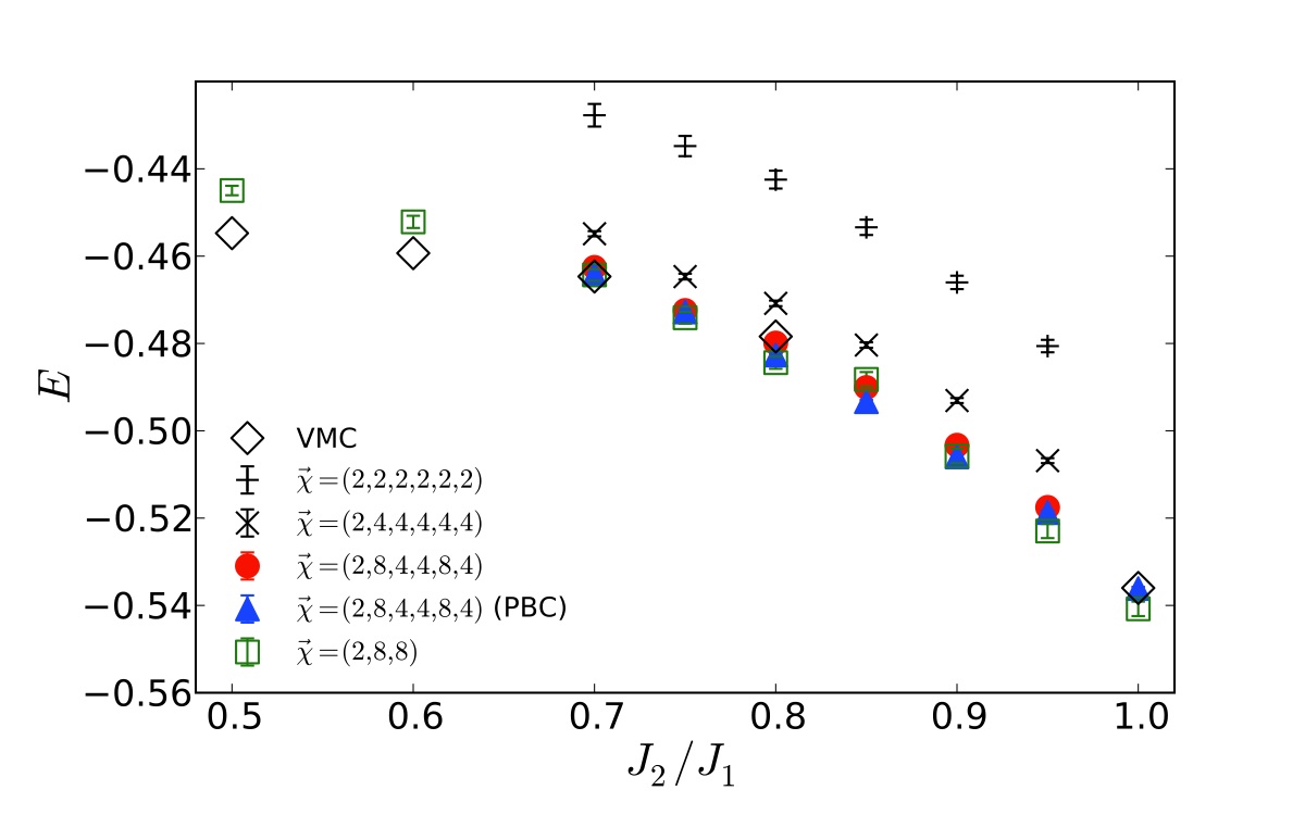
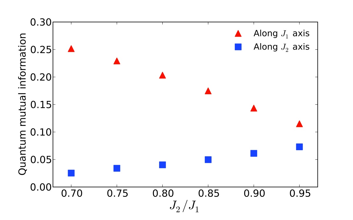
Figure 11 shows the energy per site for anisotropic cases from $J_{2}/J_{1}=0.5$ to $1.0$. The tensor sizes in the tensor network with two ER levels are $\vec{\chi}=(2,2,2,2,2,2)$, $(2,4,4,4,4,4)$, and $(2,8,4,4,8,4)$. The value of energy is improved by increasing the tensor size. In particular, the results for the MERA tensor network are better than those of VMC calculationsYunoki and Sorella (2006) in the region of $J_{2}/J_{1}\geq 0.75$. Even at $J_{2}/J_{1}=0.7$, the result of MERA by using the infinite-size scheme with two ER levels ($N=2166$) is a little (0.5%) higher than that of VMC calculationsYunoki and Sorella (2006). The difference may removed by the initial condition or by a tensor optimization process. However, the difference gets worse in the stronger anisotropic region for $J_{2}/J_{1}<0.7$. Figure 12 shows the quantum mutual information (QMI) of nearest neighbor sites along the $J_{1}$ and $J_{2}$ axes. QMI represents the quantum correlation of two sites. If there is only a classical correlation between two sites, QMI is zero. The QMI of two sites $i$ and $j$ is defined as

$$I_{ij}\equiv S_{i}+S_{j}-S_{ij},$$ (6)

where $S_{i}$ and $S_{j}$ are the entanglement entropy of site $i$ and $j$, respectively, and $S_{ij}$ is the entanglement entropy of two sites $i$ and $j$. As shown in Fig. 12, when the spatial anisotropy increases ($J_{2}/J_{1}$ decreases), the QMI along the $J_{1}$ and $J_{2}$ axes increases and decreases, respectively. However, we assume an isotropic entanglement structure in the tensor network of this study (see Fig. 3). The mismatch may cause the poor performance in the stronger anisotropic region. Therefore, in the following, we will focus on the weak anisotropic region, $J_{2}/J_{1}\geq 0.7$.

Figure 11: (Color online) Energy per site by using tensor networks with two ER levels ($N=2166$). The results of the infinite-size scheme are mainly plotted. The results of the PBC scheme with two ER levels ($N=2166$) and the infinite-size scheme with a single ER level ($N=114$) are also plotted only for the largest tensor size. The VMC results are adapted from Tables I and III in Ref. Yunoki and Sorella, 2006.

Figure 12: (Color online) Quantum mutual information of nearest neighbor sites along $J_{1}$ and $J_{2}$ axes using the infinite-size scheme with two ER levels ($N=2166$). The size of the tensors is $\vec{\chi}=(2,8,4,4,8,4)$.

III.2.3 Magnetization

Figure 13: (Color online) Average on-site magnetization and average angle between magnetic moments on $J_{2}$ links. These results are obtained using the infinite-size scheme with two ER levels ($N=2166$). The horizontal axis denotes energy per site, $E_{\rm inf}(N=2166)$. The left and right vertical axes denote magnetization, $M$, and angle between magnetic moments on $J_{2}$ links, $\theta_{2}$, respectively. Crosses, circles, and stars denote $(E_{\rm inf}(N=2166),M)$ at $J_{2}/J_{1}=0.9$, $0.8$, and $0.7$, respectively. Squares, triangle, and diamonds denote $(E_{\rm inf}(N=2166),\theta_{2})$ at $J_{2}/J_{1}=0.9,0.8,$ and $0.7$, respectively. The three curves are quadratic fittings for $(E_{\rm inf}(N=2166),M)$ points. The three lines are linear fittings for $(E_{\rm inf}(N=2166),\theta_{2})$ points. For all cases of $J_{2}/J_{1}$, the tensor sizes of the left-most, middle, and right-most points are $(\chi_{1},\chi_{2},\chi_{3},\chi_{4},\chi_{5},\chi_{6})=(2,8,4,4,8,4)$, $(2,4,4,4,4,4)$, and $(2,2,2,2,2,2)$, respectively.

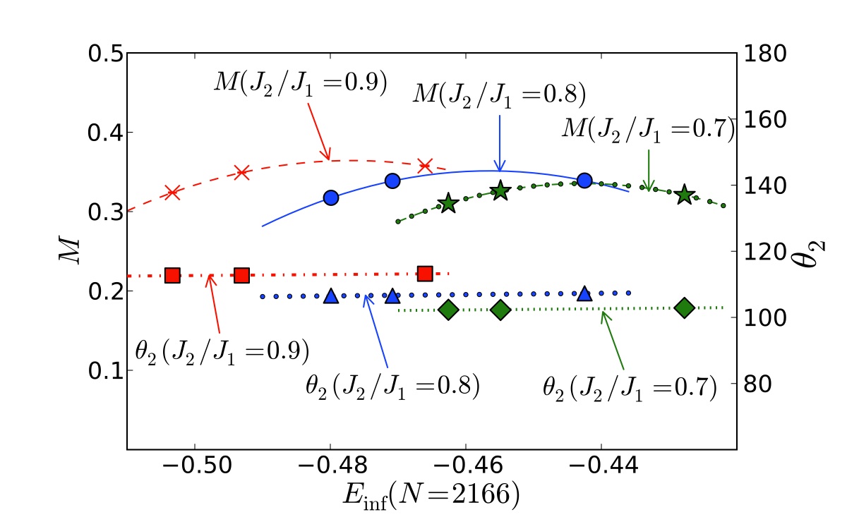
In the region $0.7\leq J_{2}/J_{1}\leq 1$, the MERA tensor network states break SU(2) symmetry and they have finite on-site magnetizations for both finite and infinite-size lattices. Figure 13 shows magnetization and the average angle between magnetic moments on $J_{2}$ links for three cases, $J_{2}/J_{1}=0.7$, $0.8$, and $0.9$, calculated using infinite-size scheme. As in the isotropic case, the dependence on tensor size remains. We cannot simply extrapolate them in the limit of the infinite dimension. However, even if the ground-state energy is about $0.1$ lower than the best results of this study, the extrapolated values from fitting curves are finite. Therefore, the results of this study suggest that the ground states are magnetic. The wave function from the infinite-size scheme is a correct quantum state in the thermodynamic limit. Thus, at least, the magnetic state is a good candidate for the ground state in this model. In recent VMC calculationsHeidarian et al. (2009), the disappearance of magnetization for $J_{2}/J_{1}\leq 0.8$ was reported. However, in the results of this study, the magnetizations smoothly change even in the region of $J_{2}/J_{1}\leq 0.8$.

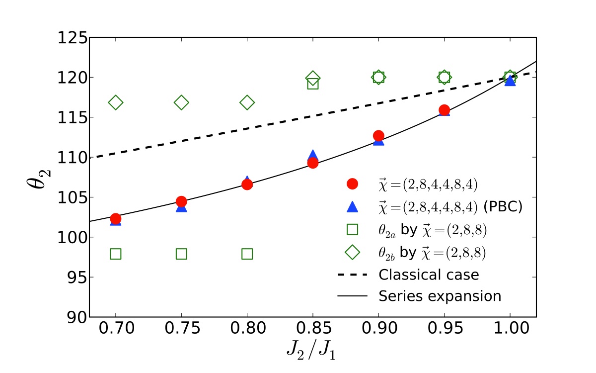
The angle between magnetic moments of nearest neighbor sites weakly depends on the tensor size, as shown in Fig. 13. There are two groups of pairs of nearest neighbor sites: One is defined on the $J_{1}$ links and the other is defined on the $J_{2}$ links. We define $\theta_{i}$ as the average angle between magnetic moments on $J_{i}$ links. In detail, $\theta_{2}$ may be split into two groups, $\theta_{2a}$ and $\theta_{2b}$, which correspond to two directions along the $J_{2}$ axis. First, in all results in the anisotropic region, the values of the sum $\theta_{1}+\theta_{2a}+\theta_{2b}$ are $359.5(6)$. Thus, all magnetic moments are coplanar, i.e., always lie on the same plane. Figure 14 shows the average angle $\theta_{2}$ of MERA tensor network states. Results only for the largest tensor size are plotted. There is no discrepancy between $\theta_{2a}$ and $\theta_{2b}$ in the cases of two ER levels. As shown by the solid (red) circles and the solid (blue) triangles in Fig. 14, the average angle smoothly changes from $115.9(2)$ to $102(2)$ when $J_{2}/J_{1}$ decreases from $0.95$ to $0.7$. Thus the wave vectors of magnetic order are incommensurate. In contrast, as shown by the open (green) squares and the open (green) diamonds in Fig. 14, the average angle suddenly changes around $J_{2}/J_{1}=0.825$ in the case of single ER. In detail, under $J_{2}/J_{1}\leq 0.8$, $\theta_{2}$ splits into $\theta_{2a}$ and $\theta_{2b}$. In other words, the reflection symmetry along the $J_{1}$ axis breaks in $J_{2}/J_{1}\leq 0.8$ by using the single ER level. Similar results have been reported in a cylindrical lattice with a width as narrow as 6 in DMRG calculationsWeichselbaum and White (2011). The reason for the behavior of angle in the case of single ER is the strong finite-size effect of the unit cell in tensor networks. Thus, a large unit cell is necessary to capture the incommensurate state. The dashed line in Fig. 14 is the angle between magnetic moments on the $J_{2}$ links for the classical spatially anisotropic antiferromagnetic Heisenberg model. It is different from the results of MERA tensor networks. The solid line in Fig. 14 shows the results of the series expansion method Zheng et al. (1999). Although the methods are very different, the series expansion results and those from the present work are in good agreement with each other. This fact gives a strong evidence for existence of a stable spiral phase. The change of wave number is larger than that of the classical one. Quantum fluctuations weaken the effective coupling between chains and enhance the incommensurability.

Figure 14: (Color online) Average angles between magnetic moments on $J_{2}$ links. The solid line denotes results of series expansion methodsZheng et al. (1999). The dotted line shows the value from the classical anisotropic triangular model.

IV Conclusions

Using ER tensor networks, we numerically studied the ground states of spin-$\frac{1}{2}$ Heisenberg antiferromagnets on anisotropic triangular lattices.

Since the area law of entanglement entropy holds in an ER tensor network, in principle, this new method may be effective for capturing high entanglement quantum states as expected in frustrated quantum magnets. Since we only assume an entanglement structure, the results of this study will serve as a new piece of evidence independent of the previous ones, with a totally new kind of bias.

Numerical results using tensor networks with one and two ER levels were reported, which correspond to $N=114$ and $N=2166$ unit cells, respectively. First, we confirmed the $120^{\circ}$ magnetic order ground state at the isotropic point $J_{1}=J_{2}$ by using a tensor network with a single ER level ($N=114$). The entanglement entropy was more sensitive to the direct product state on the top layer with a small unit cell size. Second, using the tensor network with two ER levels ($N=2166$), we found a stable spiral magnetic structure with incommensurate wave vectors at least in the anisotropic region $0.7\leq J_{2}/J_{1}<1$. In particular, the angle between magnetic moments on nearest neighbor sites agrees very well with results of the series expansion methodZheng et al. (1999), which is a very different approach.

However, the spiral phase that we found overlaps the disordered phase reported in VMC calculationsYunoki and Sorella (2006); Heidarian et al. (2009). Although we can roughly extrapolate magnetization in the limit of infinite dimension, we did not find the sharp decrease in magnetization around $J_{2}/J_{1}=0.85$ reported in the VMC calculationHeidarian et al. (2009). By increasing the dimension of tensor indices, and by modifying the structure of the ER tensor network, the author hopes that we can obtain a complete answer in the near future. In particular, to overcome the computational cost, we may need to explore less demanding methods in future studies such as combining the tensor network method with Monte Carlo samplingFerris and Vidal (2012).

In real materials such as $\kappa$-(BEDT-TTF)₂ Cu₂ (CN)₃ and EtMe₃Sb[Pd(dmit)₂]₂, high-order interaction may play an import role. In particular, models with ring exchange were discussed to explain the disordered behavior in real materialsPowell and McKenzie (2011). The ER tensor network may be useful for studying ground states of such models.