An Evaluation of Popular Copy-Move Forgery Detection Approaches
Abstract
A copy-move forgery is created by copying and pasting content within the same image, and potentially post-processing it. In recent years, the detection of copy-move forgeries has become one of the most actively researched topics in blind image forensics. A considerable number of different algorithms have been proposed focusing on different types of postprocessed copies. In this paper, we aim to answer which copy-move forgery detection algorithms and processing steps (e. g. , matching, filtering, outlier detection, affine transformation estimation) perform best in various postprocessing scenarios. The focus of our analysis is to evaluate the performance of previously proposed feature sets. We achieve this by casting existing algorithms in a common pipeline. In this paper, we examined the most prominent feature sets. We analyzed the detection performance on a per-image basis and on a per-pixel basis. We created a challenging real-world copy-move dataset, and a software framework for systematic image manipulation. Experiments show, that the keypoint-based features Sift and Surf, as well as the block-based DCT, DWT, KPCA, PCA and Zernike features perform very well. These feature sets exhibit the best robustness against various noise sources and downsampling, while reliably identifying the copied regions.
Index Terms:
Image forensics, copy-move forgery, benchmark dataset, manipulation detection, comparative studyI Introduction
The goal of blind image forensics is to determine the authenticity and origin of digital images without the support of an embedded security scheme (see e. g. [1, 2]). Within this field, copy-move forgery detection (CMFD) is probably the most actively investigated subtopic. A copy-move forgery denotes an image where part of its content has been copied and pasted within the same image. Typical motivations are either to hide an element in the image, or to emphasize particular objects, e. g. a crowd of demonstrators. A copy-move forgery is straightforward to create. Additionally, both the source and the target regions stem from the same image, thus properties like the color temperature, illumination conditions and noise are expected to be well-matched between the tampered region and the image. The fact that both the source and the target regions are contained in the same image is directly exploited by many CMFD algorithms, e. g. [3, 4, 5, 6, 7, 8, 9, 10, 11, 12, 13, 14, 15, 16, 17, 18, 19, 20, 21, 22, 23, 24, 25, 26, 27, 28]. We will briefly review existing methods in Sec. II. An example of a typical copy-move forgery is shown in Fig. 1.
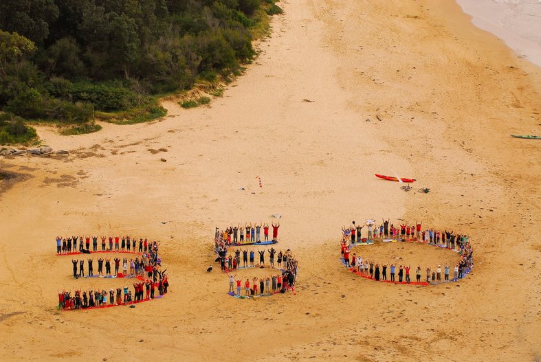

The goal of the paper is to examine which CMFD method to use under different image attributes, like different image sizes and quantities of JPEG compression. Some limited prior work already exists on this topic, e. g. [8, 29]. However, to our knowledge, the scope of such prior work is typically limited to the particular algorithm under examination. In this paper, we adopt a practitioner’s view to copy-move forgery detection. If we need to build a system to perform CMFD independent of image attributes, which may be unknown, which method should we use? For that purpose, we created a realistic database of forgeries, accompanied by a software that generates copy-move forgeries of varying complexity. We defined a set of what we believe are “common CMFD scenarios” and did exhaustive testing over their parameters. A competitive CMFD method should be able to cope with all these scenarios, as it is not known beforehand how the forger applies the forgery. We implemented feature sets that have been proposed in the literature, and integrated them in a joint pipeline with different pre- and postprocessing methods. Results show, that keypoint-based methods have a clear advantage in terms of computational complexity, while the most precise detection results can be achieved using Zernike moments [24].
The paper is organized as follows. In Sec. II, we present existing CMFD algorithms within a unified workflow. In Sec. III, we introduce our benchmark data and the software framework for evaluation. In Sec. IV we describe the employed error metrics. The experiments are presented in Sec. V. We discuss our observations in Sec. VI. Sec. VII contains a brief summary and closing remarks.
II Typical Workflow for Copy-Move Forgery Detection
Although a large number of CMFD methods have been proposed, most techniques follow a common pipeline, as shown in Fig. 2. Given an original image, there exist two processing alternatives. CMFD methods are either keypoint-based methods (e. g. [3, 11, 22]) or block-based methods (e. g. [4, 5, 6, 7, 9, 10, 12, 13, 14, 15, 16, 17, 18, 19, 20, 21, 23, 24, 25, 26, 27, 28]). In both cases, preprocessing of the images is possible. For instance, most methods operate on grayscale images, and as such require that the color channels be first merged. For feature extraction, block-based methods subdivide the image in rectangular regions. For every such region, a feature vector is computed. Similar feature vectors are subsequently matched. By contrast, keypoint-based methods compute their features only on image regions with high entropy, without any image subdivision. Similar features within an image are afterwards matched. A forgery shall be reported if regions of such matches cluster into larger areas. Both, keypoint- and block-based methods include further filtering for removing spurious matches. An optional postprocessing step of the detected regions may also be performed, in order to group matches that jointly follow a transformation pattern.

Due to differences in the computational cost, as well as the detected detail, we consider the difference between block- and keypoint-based methods very important. Thus, we separately describe these two variants for feature vector computation in the next two subsections, Sec. II-A and Sec. II-B, respectively. Additional relevant details to the remaining steps in the pipeline are presented below.
Matching
High similarity between two feature descriptors is interpreted as a cue for a duplicated region. For block-based methods, most authors propose the use of lexicographic sorting in identifying similar feature vectors (see e. g. [4, 5, 6, 7, 9, 10, 12, 13, 14, 15, 16, 17, 18, 19, 21, 23, 24, 25, 26, 27, 28]). In lexicographic sorting a matrix of feature vectors is built so that every feature vector becomes a row in the matrix. This matrix is then row-wise sorted. Thus, the most similar features appear in consecutive rows.
Other authors use the Best-Bin-First search method derived from the kd-tree algorithm [30] to get approximate nearest neighbors [11, 22, 20]. In particular, keypoint-based methods often use this approach. Matching with a kd-tree yields a relatively efficient nearest neighbor search. Typically, the Euclidean distance is used as a similarity measure. In prior work [31], it has been shown that the use of kd-tree matching leads, in general, to better results than lexicographic sorting, but the memory requirements are significantly higher. Note, however, that the dimensions of some feature sets are ordered by importance (for instance, in [32, 18, 13]). For these features, the performance gain over lexicographic sorting is minimal. In our setup we matched feature vectors using the approximate nearest neighbor method of Muja et al. [33]. It uses multiple randomized kd-trees for a fast neighbor search.
Filtering
Filtering schemes have been proposed in order to reduce the probability of false matches. For instance, a common noise suppression measure involves the removal of matches between spatially close regions. Neighboring pixels often have similar intensities, which can lead to false forgery detection. Different distance criteria were also proposed in order to filter out weak matches. For example, several authors proposed the Euclidean distance between matched feature vectors [20, 27, 24]. In contrast, Bravo-Solorio and Nandi [7] proposed the correlation coefficient between two feature vectors as a similarity criterion.
Postprocessing
The goal of this last step is to only preserve matches that exhibit a common behavior. Consider a set of matches that belongs to a copied region. These matches are expected to be spatially close to each other in both the source and the target blocks (or keypoints). Furthermore, matches that originate from the same copy-move action should exhibit similar amounts of translation, scaling and rotation.
The most widely used postprocessing variant handles outliers by imposing a minimum number of similar shift vectors between matches. A shift vector contains the translation (in image coordinates) between two matched feature vectors. Consider, for example, a number of blocks which are simple copies, without rotation or scaling. Then, the histogram of shift vectors exhibits a peak at the translation parameters of the copy operation.
Mahdian and Saic [20] consider a pair of matched feature vectors as forged if: a) they are sufficiently similar, i. e. their Euclidean distance is below a threshold, and b) the neighborhood around their spatial locations contains similar features. Other authors use morphological operations to connect matched pairs and remove outliers [28, 16, 22, 26]. An area threshold can also be applied, so that the detected region has at least a minimum number of points [19, 22, 26, 27]. To handle rotation and scaling, Pan and Lyu [22] proposed to use RANSAC. For a certain number of iterations, a random subset of the matches is selected, and the transformations of the matches are computed. The transformation which is satisfied by most matches (i. e. which yields most inliers) is chosen. Recently, Amerini et al. [3] proposed a scheme which first builds clusters from the locations of detected features and then uses RANSAC to estimate the geometric transformation between the original area and its copy-moved version. Alternatively, the Same Affine Transformation Selection (SATS) [8] groups locations of feature vectors to clusters. In principle, it performs region growing on areas that can be mapped onto each other by an affine transformation. More precisely, if the features computed on three spatially close blocks match to three feature vectors whose blocks are also spatially close, then these groups of blocks might be part of a copied region. The affine transformation to map both groups of blocks onto each other is computed. Further blocks from the neighborhood are added if the matched pairs satisfy the same affine transformation. For details, see [8]. Although not explicitly reported in this paper, we evaluated the impact of each of these methods. Ultimately, we adopted two strategies. For block-based approaches, we used a threshold based on the SATS-connected area to filter out spurious detections, as SATS provided the most reliable results in early experiments. To obtain pixel-wise results for keypoint-based methods, we combined the methods of Amerini et al. and Pan and Lyu. We built the clusters described by Amerini et al., but avoided the search for the reportedly hard to calibrate inconsistency threshold [3]. Instead, clusters stop merging when the distance to their nearest neighbors are too high, then the affine transformation between clusters is computed using RANSAC and afterwards refined by applying the gold standard algorithm for affine homography matrices [34, pp. 130]. For each such estimated transform, we computed the correlation map according to Pan and Lyu [22]. For full details on our implementation, and a more elaborate discussion on our choice of postprocessing, please refer to the supplemental material.
To summarize, we present the joint CMFD algorithm below. Given an image, the detected regions are computed as follows:
- 1.
-
2.
For block-based methods:
-
(a)
Tile the image in overlapping blocks of size , where
-
(b)
Compute a feature vector for every block .
For keypoint-based methods:
-
(a)
Scan the image for keypoints (i. e. high entropy landmarks).
-
(b)
Compute for every keypoint a feature vector . These two steps are typically integrated in a keypoint extraction algorithm like SIFT or SURF.
-
(a)
-
3.
Match every feature vector by searching its approximate nearest neighbor. Let be a matched pair consisting of features and , where , denote feature indices, and . Let denote the image coordinates of the block or keypoint from which was extracted. Then, denotes the translational difference (“shift vector”) between positions and .
-
4.
Remove pairs where , where denotes the Euclidean norm.
-
5.
Clustering of the remaining matches that adhere to a joint pattern.
-
•
For block-based methods: Let be the number of pairs satisfying the same affine transformation . Remove all matched pairs where .
-
•
For keypoint-based methods: Apply homography-based clustering as described in the paragraph above.
-
•
-
6.
If an image contains connected regions of more than connected pixels, it is denoted as tampered.
Please note that it is quite common to set the thresholds and to the same value.
II-A Block-based Algorithms
We investigated block-based features, which we considered representative of the entire field. They can be grouped in four categories: moment-based, dimensionality reduction-based, intensity-based, and frequency domain-based features (see Tab. I).
| Group | Methods | Feature-length 111Some feature-sizes depend on the block size, which we fixed to . Also note that the feature-sizes of PCA and SVD depend on the image or block content, respectively. |
| Moments | Blur [20] | |
| Hu [26] | ||
| Zernike [24] | ||
| Dimensionality reduction | PCA [23] | – |
| SVD [13] | – | |
| KPCA [4] | ||
| Intensity | Luo [19] | |
| Bravo [7] | ||
| Lin [18] | ||
| Circle [27] | ||
| Frequency | DCT [10] | |
| DWT [4] | ||
| FMT [6] | ||
| Keypoint | Sift [11],[22],[3] | |
| Surf [36],[37] |
Moment-based: We evaluated distinct approaches within this class. Mahdian and Saic [20] proposed the use of blur-invariant moments as features (Blur). Wang et al. [26] used the first four Hu moments (Hu) as features. Finally, Ryu et al. [24] recently proposed the use of Zernike moments (Zernike).
Dimensionality reduction-based: In [23], the feature matching space was reduced via principal component analysis (PCA). Bashar et al. [4] proposed the Kernel-PCA (KPCA) variant of PCA. Kang et al. [13] computed the singular values of a reduced-rank approximation (SVD). A fourth approach using a combination of the discrete wavelet transform and Singular Value Decomposition [15] did not yield reliable results in our setup and was, thus, excluded from the evaluation.
Intensity-based: The first three features used in [19] and [7] are the average red, green and blue components. Additionally, Luo et al. [19] used directional information of blocks (Luo) while Bravo-Solorio et al. [7] consider the entropy of a block as a discriminating feature (Bravo). Lin et al. [18] (Lin) computed the average grayscale intensities of a block and its sub-blocks. Wang et al. [27] used the mean intensities of circles with different radii around the block center (Circle).
Frequency-based: Fridrich et al. [10] proposed the use of coefficients of the discrete cosine transform as features (DCT). The coefficients of a discrete wavelet transform (DWT) using Haar-Wavelets were proposed as features by Bashar et al. [4]. Bayram et al. [6] recommended the use of the Fourier-Mellin Transform (FMT) for generating feature vectors.
II-B Keypoint-based Algorithms
Unlike block-based algorithms, keypoint-based methods rely on the identification and selection of high-entropy image regions (i. e. the “keypoints”). A feature vector is then extracted per keypoint. Consequently, fewer feature vectors are estimated, resulting in reduced computational complexity of feature matching and post-processing. The lower number of feature vectors dictates that postprocessing thresholds are also to be lower than that of block-based methods. A drawback of keypoint methods is that copied regions are often only sparsely covered by matched keypoints. If the copied regions exhibit little structure, it may happen that the region is completely missed. We examined two different versions of keypoint-based feature vectors. One uses the SIFT features while the other uses the SURF features (see [36]). They are denoted as Sift and Surf, respectively. The feature extraction is implemented in standard libraries. However, particular differences of keypoint-based algorithms lie in the postprocessing of the matched features, as stated in the previous section (confer also [11, 22, 3, 36, 37]).
III Benchmark Data
Since image forensics is a relatively new field, there exist only a few benchmarking datasets for algorithm evaluation. Ng et al. [38] developed a dataset that consists of automatically spliced images. In their dataset, portions of an image are quasi-randomly copied and inserted in a different image, without post-processing. Thus, the seams of the spliced regions often exhibit sharp edges. Furthermore, these splices are frequently not semantically meaningful. The CASIA dataset [39] addresses these issues. However, the majority of the images are pixels, and thus unrealistically small. Battiato et al. [40] presented a tampered image database which focuses on the evaluation of detection methods based on JPEG artifacts. These images are also of low resolution. Almost all are pixels. Other related databases have slightly different goals. For instance, the Dresden Image Database [41] is targeting methods for camera identification. Similarly, Goljan et al. [42] presented a large-scale database for the identification of sensor fingerprints.
To our knowledge, none of the existing databases is suited for an in-depth evaluation of copy-move forgery techniques. Concurrent to our work on this paper, Amerini et al. published two ground truth databases for CMFD algorithms, called MICC F220 and MICC F2000 [3]. They consist of and images, respectively. In each of these datasets, half of the images are tampered. The image size is pixels. The type of processing on the copy-move forgeries is limited to rotation and scaling. Additionally, the source files are not available. Thus, adding noise or other artifacts to the copied region is not feasible. To address these issues, we built a new benchmark database aiming at the analysis of consumer photographs. Our images were created in a two-step process.
-
1.
We selected source images and manually prepared per image semantically meaningful regions that should be copied. We call these regions snippets. Three persons of varying artistic skill manually created the snippets. When creating the snippets, we asked the artists to vary the snippets in their size. Additionally, the snippet content should be either smooth (e. g. , sky), rough (e. g. , rocks) or structured (typically man-made buildings). These groups can be used as categories for CMFD images. More details on the categorization are provided in the supplemental material. In total snippets were constructed.
-
2.
To create copy-move forgeries in a controlled setup (i. e. as the result of a parameterized algorithm), we developed a software framework to generate copy-move forgeries using the snippets. Common noise sources, such as JPEG artifacts, noise, additional scaling or rotation, are automatically included. Additionally, a pixelwise ground truth map is computed as part of this process.
When creating the forgeries, we aimed to create realistic copy-move forgeries in high-resolution pictures from consumer cameras. Here, “realistic” refers to the number of copied pixels, the treatment of the boundary pixels and the content of the snippet. The average size of an image is about pixels. In total, around of the pixels belong to tampered image regions.
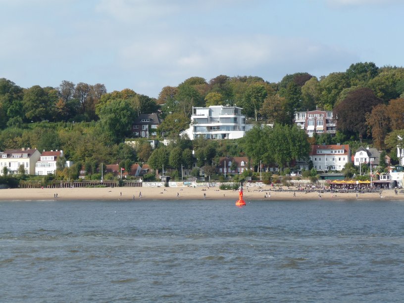
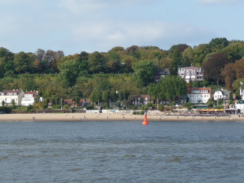
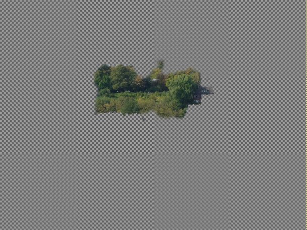
In the ground truth images, pixels are identified as either background or copy-move pixels, or as belonging to a third class of otherwise processed pixels (e. g. painted, smeared, etc.). The latter group of pixels includes border pixels of snippets where the copied data is semi-transparent, in order to form a smoother transition between the neighboring original pixels and the copied one. This is a typical process in real copy-move forgeries. Pixels that belong to this third class are not fully opaque. Fig. 3 shows a typical ground truth setup. The source image is shown on the top left, the tampered image on the top right. The snippet is shown on the bottom left, the ground truth map is shown on the bottom right. Here, white denotes copied pixels, black denotes background. The boundary pixels of the copied regions are marked gray for visualization purposes. Please note that accurate ground truth is difficult to define in such mixed data regions.

A software that can be downloaded together with the images allows the flexible combination of the original image and the tampered regions. Whenever a tampered image is created, the corresponding ground truth is automatically generated.


Various kinds of modifications can be applied to the snippet, e. g. the addition of Gaussian noise or the application of an affine transformation on the snippet. When affine transformations are used, the ground truth must be (automatically) adjusted accordingly. Care has to be taken in the case of partial occlusion of snippets. Our software framework allows multiple snippets to be arbitrarily reinserted in the image. This can result in repeated snippet overlap. See Fig. 4 for an exaggerated example. All occluded pixels have to be removed from both the source and the target snippet.


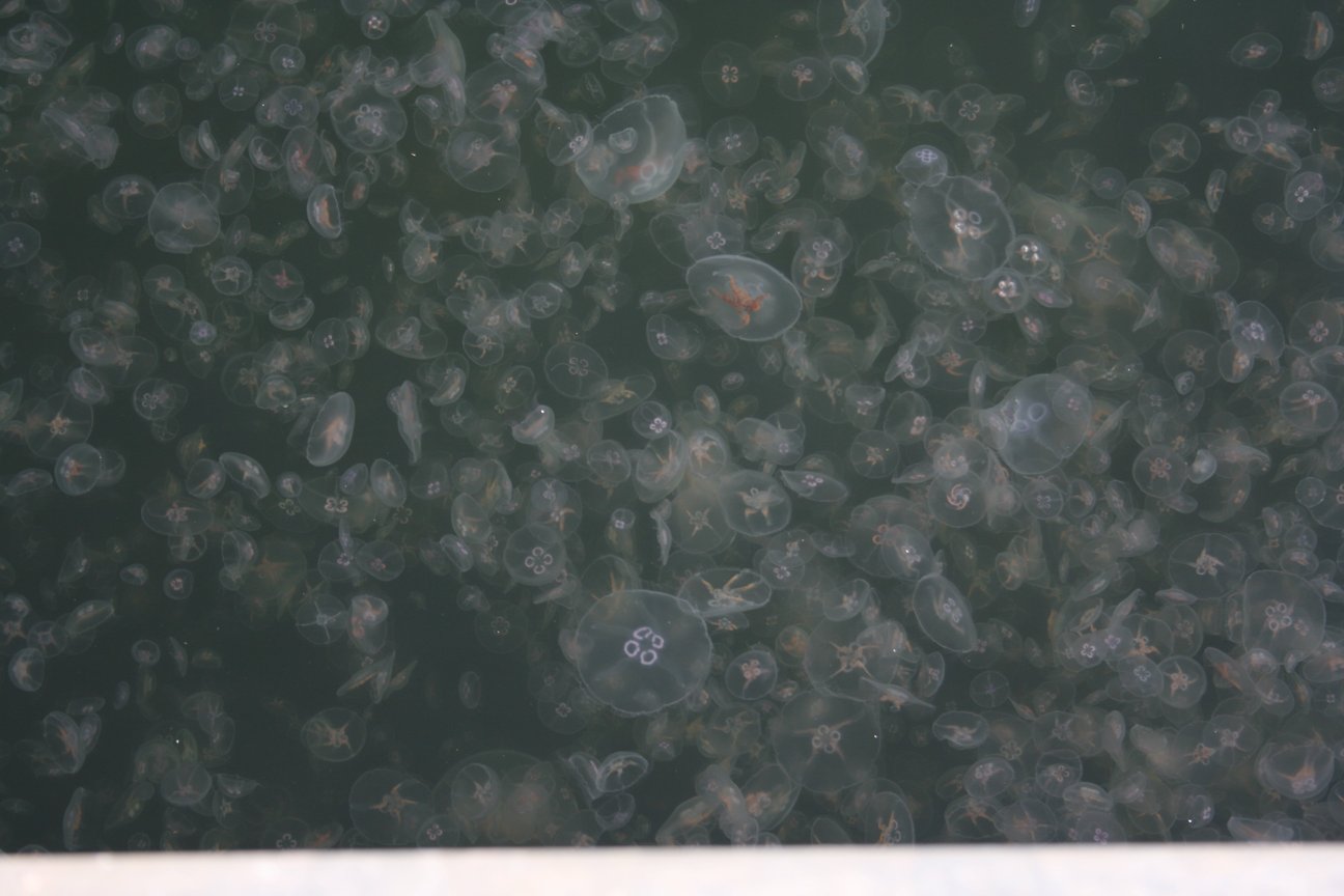
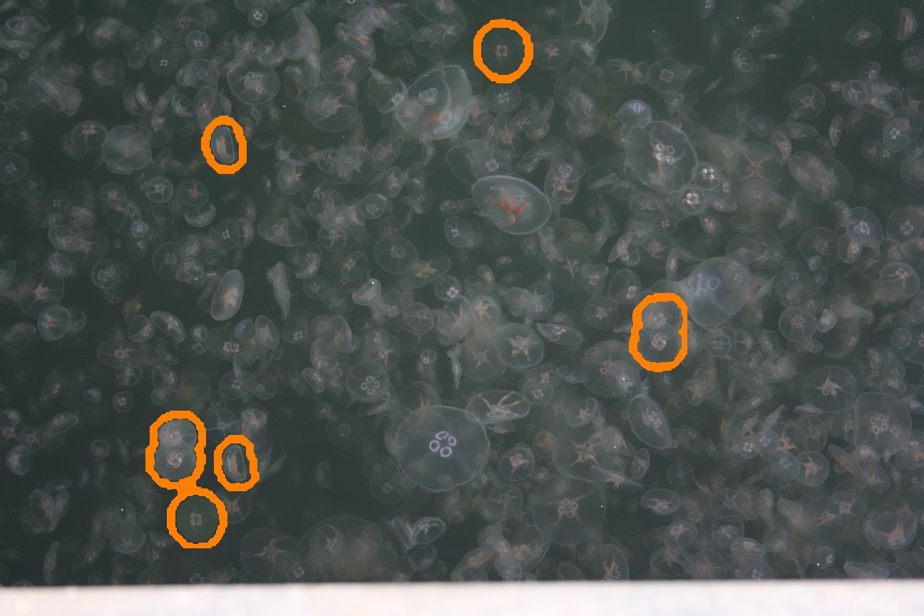
Fig. 5 shows a selection of images from the database. On the left column, the original image is shown, and on the right column the corresponding “reference manipulation”. In the top row, an example of a relatively straightforward tampering case is presented, i. e. a “large” copied area with “good” contrast. In the second example, the building in the background exhibits a high contrast, regular pattern. Here, our aim was to create a tampered image that would induce a large number of positive matches. In the third row, a very low contrast region, the cat baby, is copied. We expect keypoint-based methods to have difficulties with such test cases. The last example contains a large number of jellyfish. Here, though a single jellyfish contains considerable contrast, the sheer number of jellyfish is expected to make detection difficult. For better visualization, we highlighted the copied elements in this image.
The software together with the images can be downloaded from our web site222http://www5.cs.fau.de/.
IV Error Measures
We focused our evaluation on two performance characteristics. For practical use, the most important aspect is the ability to distinguish tampered and original images. However, the power of an algorithm to correctly annotate the tampered region is also significant, especially when a human expert is visually inspecting a possible forgery. Thus, when evaluating CMFD algorithms, we analyze their performance at two levels: at image level, where we focus on whether the fact that an image has been tampered or not can be detected; at pixel level, where we evaluate how accurately can tampered regions be identified.
IV-A Metrics
At image level, the important measures are the number of correctly detected forged images, , the number of images that have been erroneously detected as forged, , and the falsely missed forged images . From these we computed the measures Precision, , and Recall, . They are defined as:
| (1) |
Precision denotes the probability that a detected forgery is truly a forgery, while Recall shows the probability that a forged image is detected. Recall is often also called true positive rate. In the tables we also give the score as a measure which combines precision and recall in a single value.
| (2) |
We used these measures at pixel level, too. In that case, are the number of correctly detected forged pixels. denotes the number of falsely detected forged pixels and are the falsely missed pixels. The previous definition of Precision, Recall and measures also hold on the pixel level.
IV-B Protocol
Consider a CMFD algorithm that states per image whether it is tampered or not. If a copy-operation has been conducted in the image, it should raise an alarm, and vice versa. From a practical viewpoint, this can be considered the most important error measure, as the original goal – exposing digital forgeries – is directly fulfilled. However, when performance is measured on a per-image basis, the underlying reason that raised the alarm is not really considered. Image-wise performance charts do not typically distinguish between a method which correctly marks most forged areas versus a method which almost randomly marks regions.
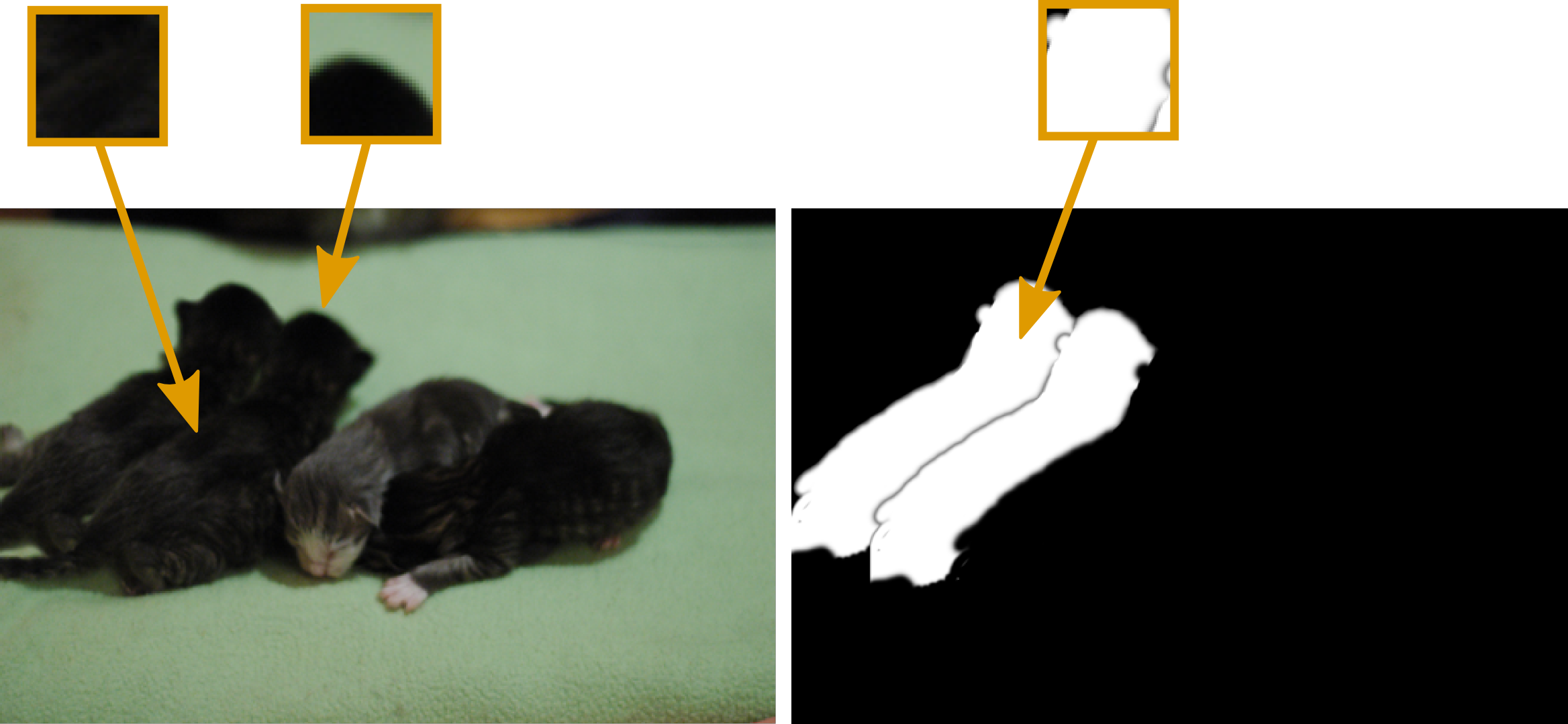
To address this issue, we conducted a second series of evaluations. Here, we examined the performance of detecting copies on a per-pixel basis. In principle, such an approach allows a much more finegrained statement about the details that a method is able to detect. Ultimately, we consider these results to offer more insight on the construction of future CMFD algorithms. However, such an evaluation requires a careful definition of ground truth, since it needs to clearly specify which pixels have been copied. This is often not a simple task. We identified three cases that need further attention. Fig. 6 illustrates these cases. It shows the tampered four copied cat babies and the generated ground truth. Three particular regions are shown as closeups. On the left window, the boundary between source and copy, consisting of black fur, is shown. The intensities of the source region, as well as the copied region, are almost indistinguishable. In such cases we draw the boundary where the target region has been inserted. This can also be seen from the grayish border between source and copy in the ground truth image. In the middle window, a closeup of the head is shown. Next to the head is the seam of the copied region. However, seams are almost always not 1-to-1 copies, but partially transparent, smeared and so on. In the ground truth image, such pixels can be recognized as being neither fully white nor fully black. We consider such pixels as not well-defined for copy-move forgery detection, as they exhibit a mixture of the copy and the original background. Thus, for the evaluation of CMFD, we excluded all such pixels. Finally, on the right window is a closeup of the ground truth. The interior of the copied area is fully white, i. e. every pixel counts for copy-move forgery detection. However, further postprocessing, e. g. added noise, or JPEG artifacts, can cause pixels in the copied region to considerably deviate from pixels in the source region. One could choose to exclude pixels that deviate significantly, but it is unclear how to accurately define a sufficient amount of deviation. Nonetheless, our goal is to examine the robustness of CMFD approaches under such disturbances. Thus, we chose to leave the ground truth “clean”, i. e. independent of any applied postprocessing.
V Experiments
In the first series of experiments, we evaluated the detection rate of tampered images. In the second series, we evaluated pixelwise the detection of copied regions, in order to obtain a more detailed assessment of the discriminative properties of the features. In total, we conducted experiments with about variants of the forged image (e. g. different scales of snippets, different rotation angles of snippets, different compression rates and their combinations) in order to better understand the behavior of the different feature sets. The complete result tables, as well as the source code to generate these results, are also available from our web site.
V-A Threshold Determination
Thresholds that are specific to a particular feature set were manually adjusted to best fit the benchmark dataset. Most threshold values for the processing pipeline (according to Sec. II) were fixed across the different methods, when possible, to allow for a fairer comparison of the feature performance.
Block size : We chose to use a block size of pixels. We found this to be a good trade-off between detected image details and feature robustness. Note that the majority of the original methods also proposed a block size of pixels.
Minimum Euclidean distance : Spatially close pixels are closely correlated. Thus, matches between spatially close blocks should be avoided. In our experiments, we set the minimum Euclidean distance between two matched blocks to pixels. Thus, note that we are unable to detect copies when the pixels are moved for less than pixels. However, given the high resolution of the benchmark images, this limitation is not relevant for this work.
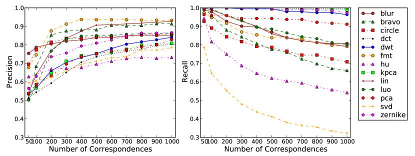
Minimum number of correspondences : This threshold reflects the minimum number of pairs which have to fulfill the same affine transformation between the copied and the pasted region. Thus, it compromises between improved noise suppression, and false rejection of small copied regions. strongly depends on the features, as some features generate denser result maps than others. Consequently, has to be chosen for each feature individually. We empirically determined appropriate values as follows. From our dataset, we created CMFD benchmark images with JPEG quality levels between and in steps of . Thus, we evaluated on the tampered images for images. The JPEG artifacts should simulate a training set with slight pixel distortions. Per block-based feature, we estimated by optimizing the -measure at image level. The results of the experiment are shown in Fig. 7. Please note that throughout the experiments, we were sometimes forced to crop the -axis of the plots, in order to increase the visibility of the obtained results. The feature set-specific values for are listed in the rightmost column of Tab. V-B1. For the sparser keypoint-based methods, we require only correspondences.
Area threshold : In our experiments, we set for the block-based methods and for the keypoint-based methods to remove spurious matches333Alternatively, it would be possible to set the threshold for keypoint matching stricter, and then to omit completely. However, we preferred this variant (i. e. a more lenient matching threshold) in order to gain better robustness to noise..
Individual feature parameters: We omitted the Gaussian pyramid decomposition for the Hu-Moments (in contrast to the original proposition [26]). This variant yields better results gave better results on our benchmark data. For Circle, we had to use a different block size , as this feature set requires an odd sized blocks for the radius computation. For KPCA, two parameters had to be determined, namely the number of samples and the variance of the Gaussian kernel . We set up a small experiment with two images (with similar proportions as images from our database) in which for both images a block of size was copied and pasted. Then we varied the parameters and chose the best result in terms of the -measure. We observed that with increasing and the results became slightly better. We empirically determined that values of and offer an overall good performance. Note that, these values are larger than what Bashar et al. [4] used. For the remaining features, we used the parameters as suggested in the respective papers.
V-B Detection at Image Level
We split these experiments in a series of separate evaluations. We start with the baseline results, i. e. direct 1-to-1 copies (no postprocessing) of the pixels. Subsequent experiments examine the cases of: noise on the copied region, JPEG compression on the entire image, rotation and scaling of the copied region.
V-B1 Plain Copy-Move
| Method | Precision | Recall | ||
| Blur | 88.89 | 100.00 | 94.12 | 100 |
| Bravo | 87.27 | 100.00 | 93.20 | 200 |
| Circle | 92.31 | 100.00 | 96.00 | 200 |
| DCT | 78.69 | 100.00 | 88.07 | 1000 |
| DWT | 84.21 | 100.00 | 91.43 | 1000 |
| FMT | 90.57 | 100.00 | 95.05 | 200 |
| Hu | 67.61 | 100.00 | 80.67 | 50 |
| KPCA | 87.27 | 100.00 | 93.20 | 1000 |
| Lin | 94.12 | 100.00 | 96.97 | 400 |
| Luo | 87.27 | 100.00 | 93.20 | 300 |
| PCA | 84.21 | 100.00 | 91.43 | 1000 |
| Sift | 88.37 | 79.17 | 83.52 | 4 |
| Surf | 91.49 | 89.58 | 90.53 | 4 |
| SVD | 68.57 | 100.00 | 81.36 | 50 |
| Zernike | 92.31 | 100.00 | 96.00 | 800 |
| Average | 85.54 | 97.92 | 90.98 | – |
As a baseline, we evaluated how the methods perform under ideal conditions. We used the original images, and spliced images without any additional modification. We chose per-method optimal thresholds for classifying these images. Interestingly, although the sizes of the images and the manipulation regions vary greatly on this test set, out of the tested features perfectly solved this CMFD problem with a recall-rate of (see Tab. V-B1). However, only four methods have a precision of more than . This means that most of the algorithms, even under these ideal conditions, generate some false alarms. This comes mainly from the fact that the images in the database impose diverse challenges, and the large image sizes increase the probability of false positive matches.
V-B2 Robustness to Gaussian noise
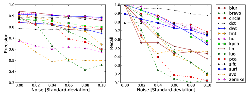
We normalized the image intensities between and and added zero-mean Gaussian noise with standard deviations of , , , and to the inserted snippets before splicing. Besides the fact that a standard deviation of leads to clearly visible artifacts, out of features drop to under recall rate, while the precision decreases only slightly, see Fig. 8(a). DCT exhibits a remarkably high recall, even when large amounts of noise are added. PCA, Sift, Surf and Hu also maintain their good recall, even after the addition of large amounts of noise. At the same time, several methods exhibit good precision. Among these, Surf provides a good balance between precision and recall, followed by PCA.
V-B3 Robustness to JPEG compression artifacts
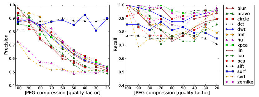
We introduced a common global disturbance, JPEG compression artifacts. The quality factors varied between and in steps of , as provided by libjpeg444http://libjpeg.sourceforge.net/. Per evaluated quality level, we applied the same JPEG compression to forgeries and complementary original images. For very low quality factors, the visual quality of the image is strongly affected. However, we consider at least quality levels down to as reasonable assumptions for real-world forgeries. Fig. 8(b) shows the results for this experiment. The precision of Surf and Sift remains surprisingly stable, while block-based methods slowly degenerate to a precision of . On the other hand, many block-based methods exhibit a relatively high recall rate, i. e. miss very few manipulations. Among these, KPCA, DCT, Zernike, Blur and PCA constantly reach a recall of or higher.
V-B4 Scale-invariance
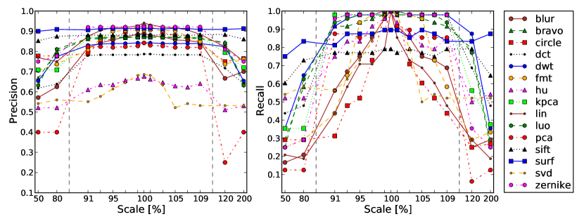
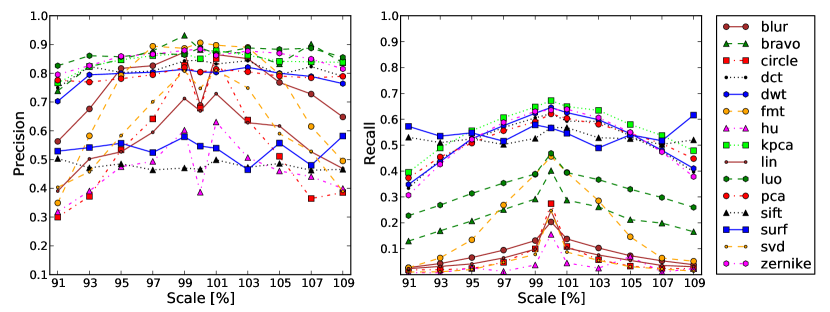
One question that recently gained attention was the resilience of CMFD algorithms to affine transformations, like scaling and rotation. We conducted an experiment where the inserted snippet was slightly rescaled, as is often the case in real-world image manipulations. Specifically, we rescaled the snippet between and of its original size, in steps of . We also evaluated rescaling by , , and to test the degradation of algorithms under larger amounts of snippet resizing. Note that we only scaled the copied region, not the source region. Fig. 8(c) shows the results for this experiment. Most features degenerate very fast at low rates of up- or down-sampling. Some methods, namely KPCA, Zernike, Luo, DWT, DCT and PCA are able to handle a moderate amount of scaling. For more extreme scaling parameters, keypoint-based methods are the best choice: their performance remains relatively stable across the whole scaling parameters.
V-B5 Rotation-invariance
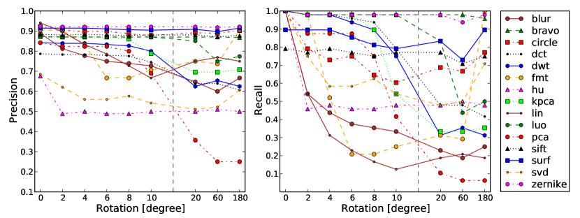
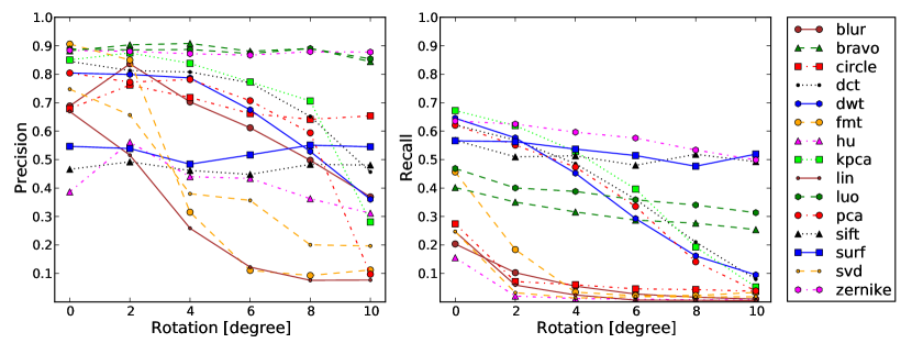
Similar to the previous experiment, we rotated the snippet between to , in steps of , and also tested three larger rotation angles of , and . In prior work [8, 31], we already showed that Zernike, Bravo and Circle are particularly well-suited as rotation-invariant features. Our new results, computed on a much more extensive data basis, partially confirm this. Fig. 8(d) shows the results. Zernike features provide the best precision, followed by Surf, Circle, Luo and Bravo. In the recall-rate, Bravo and Zernike yield consistently good results and thus seem to be very resilient to rotation. For small amounts of rotation, KPCA and Luo perform also strongly, for higher amounts of rotation, Surf features perform best. FMT, Lin, Hu and Blur seem not to be well suited to handle variations of rotation.
V-B6 Robustness to Combined Transformation
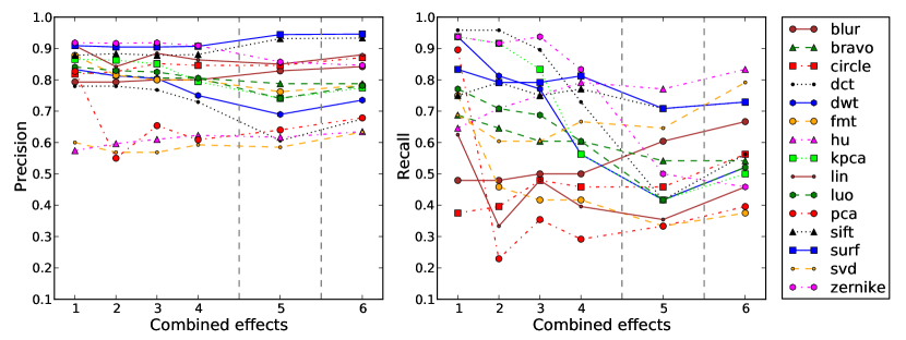
In this experiment, we examined the performance under several joint effects. We rotated the snippet by , scaled it up by and compressed the image with a JPEG-compression level of . In three subsequent setups, we increased per step the rotation by , increased scaling by , and decreased the JPEG quality by points. In setup and , slightly stronger parameters were chosen: rotation was set to and , scaling was set to and , and JPEG quality was set to and , respectively. Fig. 9 shows that high precision can be achieved for several feature sets. The best recall for small variations is achieved by DCT and Zernike. For the fourth step, Surf and Sift are almost on a par with Zernike. Note that also in the fourth step, a number of features exhibit a recall below , and can thus not be recommended for this scenario. For large rotations and scaling in the combined effects (see the scenarios and ), Sift and Surf show best precision and very good recall.
V-C Detection at Pixel Level
A second series of experiments considers the accuracy of the features at pixel level. The goal of this experiment is to evaluate how precisely a copy-moved region can be marked. However, this testing has a broader scope, as it is directly related with the discriminating abilities of a particular feature set. Under increasingly challenging evaluation data, experiments on per-match level allow one to observe the deterioration of a method in greater detail. We repeated the experiments from the previous subsections, with the same test setups. The only difference is that instead of classifying the image as original or manipulated, we focused on the number of detected (or missed, respectively) copied-moved matches.
For each detected match, we check the centers of two matched blocks against the corresponding (pixelwise) ground truth image. All boundary pixels are excluded from the evaluation (see also Fig. 3). Please note that all the measures, e. g. false positives and false negatives, are computed using all the pixels in the tampered images only. Note also, that it is challenging to make the pixelwise comparison of keypoint- and block-based methods completely fair: as keypoint-based matches are by nature very sparse, we are not able to directly relate their pixel-wise performance to block-based methods. Thus, we report the postprocessed keypoint matches (as described in Sec. II).
V-C1 Plain Copy-Move
Tab. V-C1 shows the baseline results for the dataset at pixel level. Similarly to the experiment at image level, all regions have been copied and pasted without additional disturbances. Note that we calibrated the thresholds for all methods in a way that yields very competitive (comparable) detection performances.
V-C2 Robustness to Gaussian noise
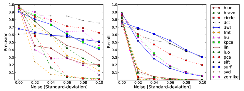
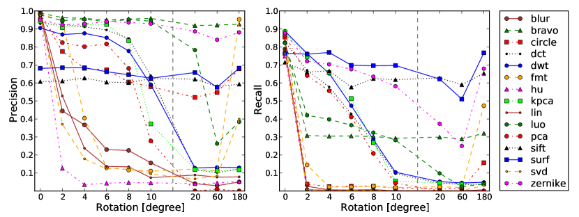
We used the same experimental setup as in the per-image evaluation, i. e. zero-mean Gaussian noise with standard deviations between and has been added to the copied region. The goal is to simulate further postprocessing of the copy. At pixel level, this experiment shows a clearer picture of the performance of the various algorithms (see Fig. 10(a)). DCT, Sift and Surf provide the best recall. DCT also outperforms all other methods with respect to precision. The performance of the remaining features splits in two groups: Circle, Blur, Bravo, SVD and Hu are very sensitive to noise, while PCA, Zernike, KPCA and DWT deteriorate slightly more gracefully.
V-C3 Robustness to JPEG compression artifacts
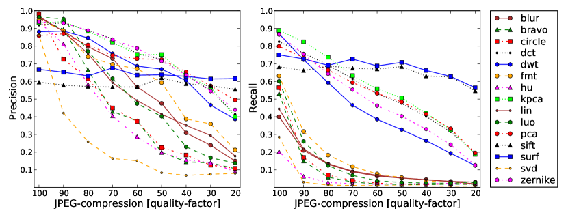
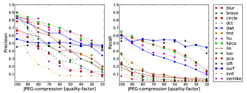
We again used the same experimental setup as in the per-image evaluation, i. e. added JPEG compression between quality levels and . Fig. 10(b) shows the resilience at pixel level against these compression artifacts. The feature sets forms two clusters: one that is strongly affected by JPEG compression, and one that is relatively resilient to it. The resilient methods are Sift, Surf, KPCA, DCT, PCA, Zernike, and slightly worse, DWT. The robustness of DCT was foreseeable, as DCT features are computed from the discrete cosine transform, which is also the basis of the JPEG algorithm.
V-C4 Scale-invariance
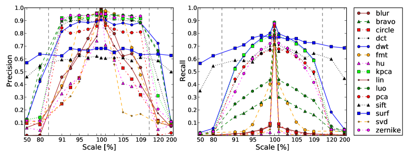
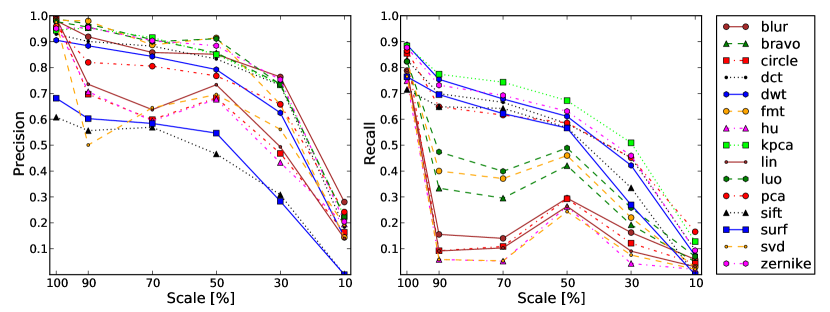
The experimental setup is the same as on the per-image level analysis. The copy is scaled between and of its original size in increments of . Additionally, we evaluated more extreme scaling parameters, namely , , and . As Fig. 10(c) shows, feature sets exhibit scaling invariance for small amounts of scaling. However, the quality strongly varies. The best performers within these feature sets are DWT, KPCA, Zernike, PCA and DCT. However, for scaling differences of more than , the keypoint-based features Sift and Surf are the only features sets that preserve acceptable precision and recall.
V-C5 Rotation-invariance
We evaluated cases where the copied region has been rotated between and (in steps of ), as well as for , and . We assumed this to be a reasonable range for practical tampering scenarios. Fig. 10(d) shows the results. Most feature sets show only weak invariance to rotation. Similar to the scaling scenario, Sift and Surf exhibit the most stable recall. From the block-based methods, Zernike, and also Bravo and Luo are the best features for larger amounts of rotation. Note that for the special case of , also FMT and and Circle perform very well.
V-C6 Robustness to Combined Transformation
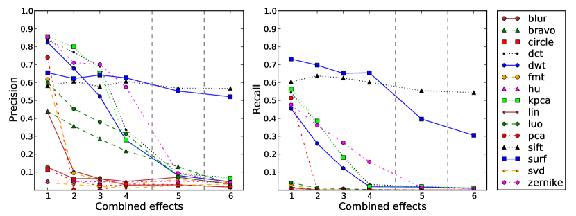
Besides the targeted study of single variations in the copied snippet, we conducted an experiment for evaluating the joint influence of multiple effects. Thus, we analyzed images where the copied part was increasingly scaled, rotated and JPEG-compressed. The setup was the same as on image level. Thus, scaling varied between and in steps of , rotation between and in steps of , and the JPEG quality ranges from to in steps of . Setup and have different parameters, namely a rotation of and , a scaling of and , and the quality of JPEG compression was set to and , respectively. The performance results are shown in Fig. 11. In these difficult scenarios, Surf and Sift perform considerably well, followed by Zernike, DCT, KPCA and DWT. Note that it is infeasible to cover the whole joint parameter space experimentally. However, we take this experiment as an indicator, that the results of the prior experiments approximately transfer to cases where these transformations jointly occur.
V-D Detection of Multiple Copies
In recent work, e. g. [3], the detection of multiple copies of the same region has been addressed. While at image level it typically suffices to recognize whether something has been copied, multiple-copies detection requires that all copied regions be identified. For such an evaluation, we modified the feature matching as follows. Instead of considering the nearest neighbor, we implemented the g2NN strategy by [3]. This method considers not only the single best-matching feature, but the best-matching features for detecting multiple copies. Although our dataset contains a few cases of single-source multiple-copies, we created additional synthetic examples. To achieve this, we randomly chose for each of the images a block of pixels and copied it times.
Tab. V-D shows the results for this scenario at pixel level. On the left side, we used the same postprocessing method as in the remainder of the paper, i. e. we matched the single nearest neighbor. On the right side, we present the results using the g2NN strategy. For many feature sets, precision slightly decreases using g2NN. This is not surprising, as many more combinations of matched regions are now possible, thus also increasing the chance for false matches. Still, some methods alike Blur, Bravo, etc. are relatively unaffected by this change in postprocessing, while others experience a remarkable performance boost. In particular, DCT, DWT, KPCA, PCA, Zernike, i. e. the strong feature sets in the prior experiments, can significantly benefit from the improved matching opportunities of g2NN. As we discuss later (see Sec. VI), we see this as yet another indicator that these features exhibit very good discriminating properties. The performance of Sift and Surf drops considerably, mainly due to the fact that the random selection of small blocks often yields regions with very few matched keypoints. Although not explicitly evaluated, we expect that selecting copy regions with high entropy (instead of a random selection), would considerably improve the detection rates of Sift and Surf.
V-E Downsampling: Computational Complexity versus Detection Performance
The evaluated methods vary greatly in their demand for resources. One widely-used workaround is to rescale images to a size that is computationally efficient. However, this raises the issue of performance degradation. In order to analyze the effects of downsampling, we scaled down all noise-free, one-to-one (i. e. without further postprocessing) forgeries from our database in steps of of the original image dimensions. Note that the detection parameters, as in the whole section, were globally fixed to avoid overfitting. In this sense, the results in this section can be seen as a conservative bound on the theoretically best performance. We observe that the performance of all features considerably drops. When downsampling by a factor of exactly , results are still better than for other scaling amounts (see Fig. 12(a) for more details). This shows that global resampling has considerable impact on the results. Some feature sets are almost rendered unusable. KPCA, Zernike, DWT, PCA, DCT, Luo, FMT and Bravo perform relatively well. Sift and Surf exhibit slightly worse precision, which might also be due to a suboptimal choice of with respect to the reduced number of keypoints in the downscaled images. However, the recall rates are competitive with the block-based methods. For completeness, we repeated the analysis of subsections V-C3, V-C4 and V-C5 on a downsampled () version of the tampered images. The results are presented in Fig. 12(b) to Fig. 12(d). The general shape of the performance curves is the same as in the previous sections. Note that the performance of recall is more strongly affected by downscaling than precision.
V-F Resource Requirements
For block-based methods, the feature-size (see Tab. I) can lead to very high memory use. For large images, this can reach several gigabytes. Tab. V (right column) shows the per-method minimum amount of memory in MB on our largest images, obtained from multiplying the length of the feature vector with the number of extracted blocks. In our implementation, the effective memory requirements were more than a factor of higher, leading to peak memory usage for DCT and DWT of more than 20GB. Note however, that the feature size of DCT and DWT depends on the block size. For better comparability, we kept the block size fixed for all methods. Within a practical setup, the block size of these feature sets can be reduced. Alternatively, the feature sets can be cropped to the most significant entries. Some groups explicitly proposed this (e. g. [23], [4]). In our experiments, as a rule of thumb, 8GB of memory sufficed for most feature sets using OpenCV’s555http://opencvlibrary.sourceforge.net/ implementation for fast approximate nearest neighbor search.
The computation time depends on the complexity of the feature set, and on the size of the feature vector. Tab. V shows the average running times in seconds over the dataset, split into feature extraction, matching and postprocessing. Among the block-based methods, the intensity-based features are very fast to compute. Conversely, Blur, DCT and KPCA features are computationally the most costly in our unoptimized implementation. The generally good-performing feature sets PCA, FMT and Zernike are also relatively computationally demanding.
| Method | Feature | Matching | Postpr. | Total | Mem. |
|---|---|---|---|---|---|
| Blur | 12059.66 | 4635.98 | 12.81 | 16712.19 | 924.06 |
| Bravo | 488.23 | 5531.52 | 156.27 | 6180.42 | 154.01 |
| Circle | 92.29 | 4987.96 | 19.45 | 5103.43 | 308.02 |
| DCT | 28007.86 | 7365.53 | 213.06 | 35590.03 | 9856.67 |
| DWT | 764.49 | 7718.25 | 119.66 | 8606.50 | 9856.67 |
| FMT | 766.60 | 6168.73 | 8.07 | 6948.03 | 1732.62 |
| Hu | 7.04 | 4436.63 | 5.36 | 4452.77 | 192.51 |
| KPCA | 6451.34 | 7048.83 | 88.58 | 13592.08 | 7392.50 |
| Lin | 12.41 | 4732.88 | 36.73 | 4785.71 | 346.52 |
| Luo | 42.90 | 4772.67 | 119.04 | 4937.81 | 269.52 |
| PCA | 1526.92 | 4322.84 | 7.42 | 5861.01 | 1232.08 |
| Sift | 15.61 | 126.15 | 469.14 | 610.96 | 17.18 |
| Surf | 31.07 | 725.68 | 295.34 | 1052.12 | 19.92 |
| SVD | 843.52 | 4961.11 | 7.65 | 5816.15 | 1232.08 |
| Zernike | 2131.27 | 4903.59 | 27.23 | 7065.18 | 462.03 |
| Average | 3549.41 | 4829.22 | 105.72 | 8487.63 | 2266.43 |
Keypoint-based methods excel in computation time and memory consumption. Their feature size is relatively large. However, the number of extracted keypoints is typically an order of magnitude smaller than the number of image blocks. This makes the whole subsequent processing very lightweight. On average, a result can be obtained within minutes, with a remarkably small memory footprint.
V-G Qualitative Results
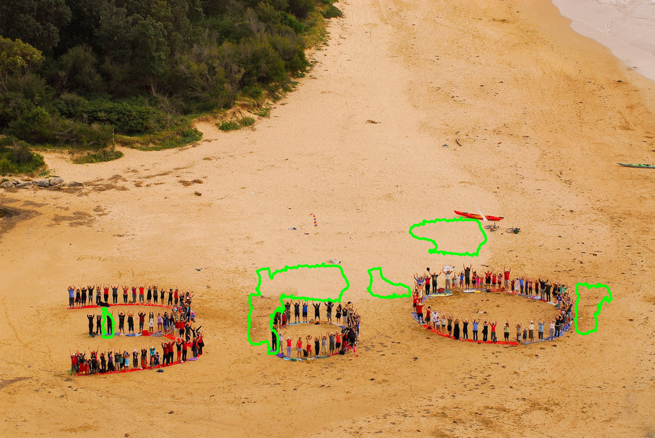
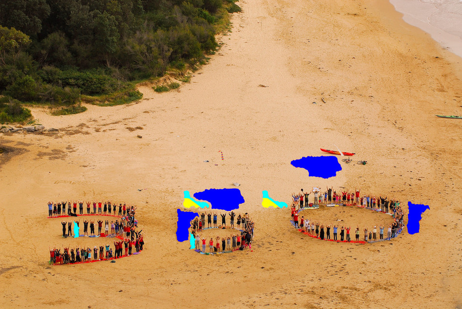
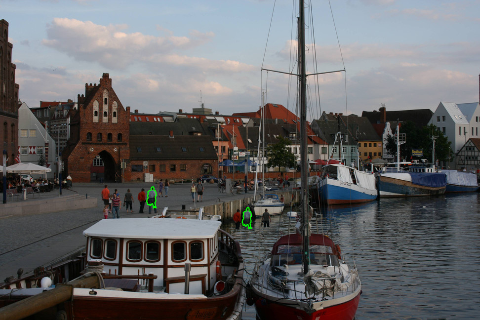
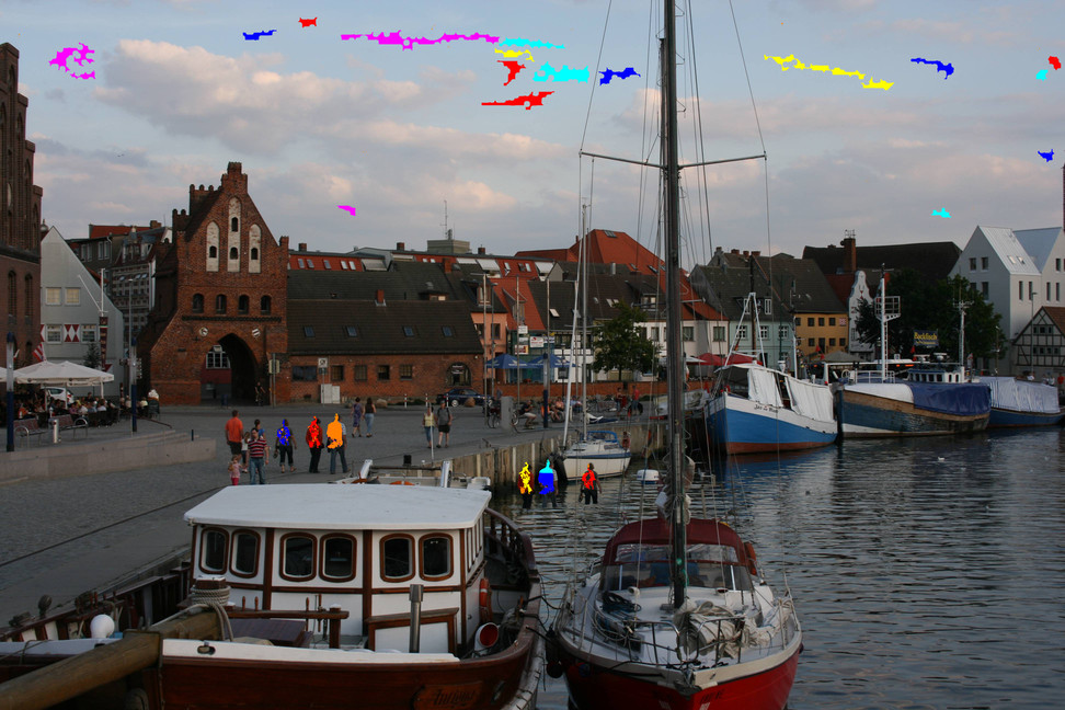
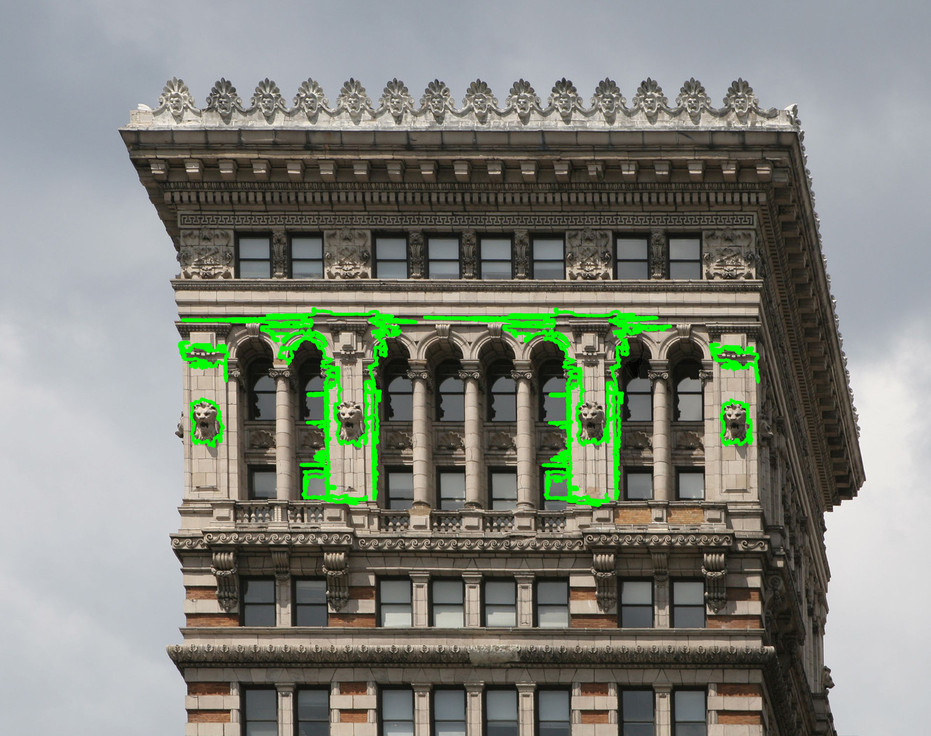
A more intuitive presentation of the numerical results is provided for four selected examples, shown in Fig. 13. On the left, the extracted contours of the keypoint-based method Surf are shown. On the right the matches detected by the block-based Zernike features are depicted. Matched regions are highlighted as brightly colored areas. In the top image, the people which formed the top of the “” (see Fig. 1) were covered by a region copied from the right side of the image. Additionally the circle was closed by copying another person. Surf and Zernike correctly detected all copied regions. In the second row, three passengers were copied onto the sea. The image was afterwards compressed with JPEG quality . Surf yielded one correct match but misses the two other persons. Zernike marked all passengers correctly. However, it also generated many false positives in the sky region.
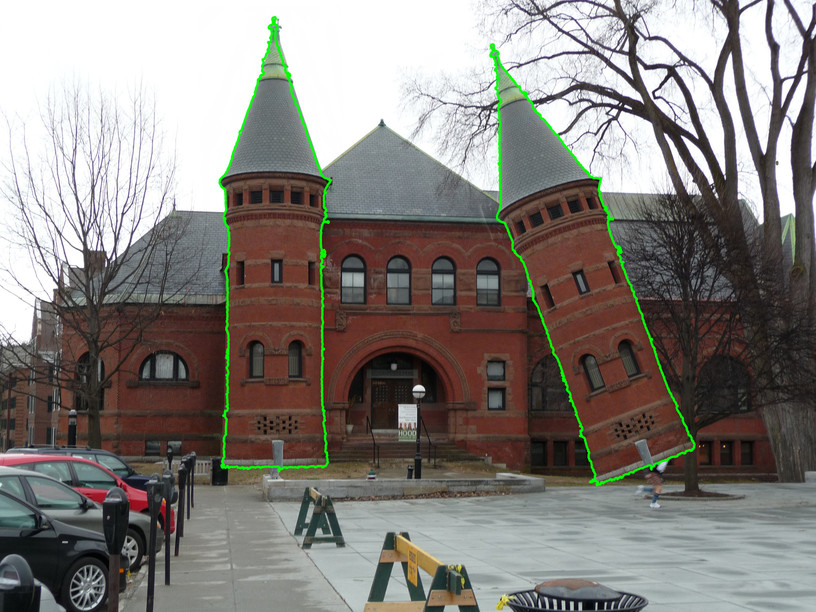
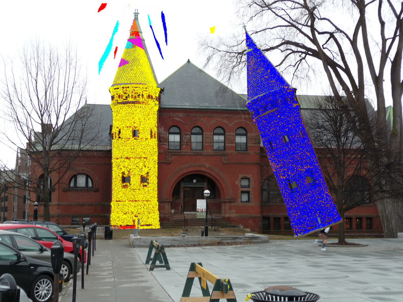
In the third image, a rotation was applied to the copy of the tower. Both methods accurately detected the copied regions. This observation is easily repeatable as long as: a) rotation-invariant descriptors are used, and b) the regions are sufficiently structured. As with JPEG-compression Zernike produced some false positives above the left tower. In the bottom row, the two stone heads at the edge of the building were copied in the central part. Each snippet was rotated by and scaled by . The entire image was then JPEG compressed at a quality level of . This image is particularly challenging for keypoint-based methods, as it contains a number of high-contrast self-similarities of non-copied regions. Zernike clearly detected the two copies of the stone heads. Surf also detected these areas, but marked a large number of the background due to the background symmetries.

V-H Results by Image Categories
To investigate performance differences due to different texture of the copied regions, we computed the performances according to categories. We subdivided the dataset into the object class categories living, manmade, nature and mixed. Although man-made exhibited overall the best performance, the differences between the categories were relatively small. This finding is in agreement with the intuition that the descriptors operate on a lower level, such that object types do not lead to significant performance differences. In a second series of experiments, we used the artists’ categorization of the snippets into smooth, rough and structure (see III). Overall, these results confirm the intuition that keypoint-based methods require sufficient entropy in the copied region to develop their full strength. In the category rough, Sift and Surf are consistently either the best performing features or at least among the best performers. Conversely, for copied regions from the category smooth, the best block-based methods often outperform Surf and Sift at image or pixel level. The category structure ranges between these two extremes. The full result tables for both categorization approaches can be found in the supplemental material.
VI Discussion
We believe that the obtained insights validate the creation of a new benchmark dataset. The selection of the evaluation data for the CMFD algorithms is a non-trivial task. To our knowledge, all existing test sets are somewhat limited in one aspect or another. For instance, preliminary experiments suggested that image size strongly influences the detection result of CMFD algorithms. One workaround is to scale every input image to a fixed size. However, as we show in Fig. 12, interpolation itself influences the detection performance. Furthermore, in the case of downsampling, the size of the tampered region is also reduced, further inhibiting detection. Thus, we conducted all experiments, unless otherwise stated, in the full image resolution (note, however, that the images themselves had different sizes, ranging from pixels to pixels). This greatly increased the risk of undesired matches in feature space, especially when a feature set exhibits weak discriminative power. Consequently, differences in the feature performance became more prominent.
Which CMFD method should be used? During the experiments, we divided the proposed methods in two groups. Surf and Sift, as keypoint-based methods, excel in computation time, memory footprint. The advantage in speed is so significant, that we consider it worth applying these methods always, independent of the detection goal. Tab. V-B1 and subsequent experiments indicate slightly better result for Surf than for Sift. When a copied area has undergone large amounts of rotation or scaling, Sift and Surf are clearly the best choices. One should be aware that keypoint-based methods often lack the detail for highly accurate detection results. When regions with little structure are copied, e. g. the cats image in Fig. 5, keypoint-based methods are prone to miss them. In contrast, highly self-similar image content, as the building in Fig. 13 can provoke false positive matches.
The best-performing block-based features can relatively reliably address these shortcomings. Experiments on per-image detection indicate that several block-based features can match the performance of keypoint-based approaches. We conducted additional experiments to obtain stronger empirical evidence for the superiority of one block-based method over another. These experiments measured the pixelwise precision and recall of the block-based approaches. Experiments on the robustness towards noise and JPEG artifacts showed similar results. DCT, PCA, KPCA, Zernike and DWT outperformed the other methods by a large margin w.r.t. recall. Their precision also outperformed the other block-based methods for large amounts of noise and heavy JPEG compression. As shown for example in Fig. 13, a good precision leads to a low number of false positive matches. When the copied region is scaled, the aforementioned five block-based features also perform well for small amounts of scaling. Note, however, that we were not able to obtain good results with block-based methods using larger scaling parameters. For rotated copies, Zernike, Luo and Bravo, DWT, KPCA, DCT and PCA can handle small degrees of rotation very well. In general, for detecting rotated copies, Zernike performed remarkably well.
In a more practical scenario, running a block-based CMFD algorithm on full-sized images can easily exceed the available resources. Thus, we examined, how block-based algorithms perform when the examined image is downsampled by the investigator to save computation time. Not surprisingly, the overall performance drops. However, the best performing feature sets remain relatively stable, and confirm the previous results only at a lower performance level.
In all the previous discussion, we tailored our pipeline for the detection of a single one-to-one correspondence between source region and copied region. However, we also evaluated, at a smaller scale, the detection of multiple copies of the same region. We adapted the matching and filtering steps to use g2NN, as proposed by Amerini et al. [3], so that the best-matching features were considered. Interestingly, the already good features DCT, DWT, KPCA, PCA and Zernike profited the most from the improved postprocessing. This re-emphasizes the observation that these feature sets are best at capturing the relevant information for CMFD. With the improved postprocessing by Amerini et al., the advantages of these features can be fully exploited.
In a practical setup, one should consider a two-component CMFD system. One component involves a keypoint-based system, due to its remarkable computational efficiency, small memory footprint and very constant performance. This allows for instance the screening of large image databases. The second component should be a block-based method, for close and highly reliable examination of an image. In particular when the added noise or transformations to the copied area are small, block-based methods are considerably more accurate. We consider Zernike features as a good choice for this component. For a block-based method, its memory and runtime requirements are low, compared to the detection performance.
Note, however, that a final recommendation has of course to be made based upon the precise detection scenario. We assume that the provided performance measurements, together with the publicly available dataset, can greatly support practitioners and researchers to hand-tailor a CMFD pipeline to the task at hand. For instance, one could imagine a fusion-based system, consisting of the best features from each category. Alternatively, other forensic tools, like resampling detection or detection of double JPEG compression can compensate the current shortcomings of existing CMFD approaches (see, e. g. [1]). For instance, under moderate degrees of JPEG compression, rescaled or rotated copies reliably exhibit traces of resampling. Thus, rotation- and scaling invariant CMFD can be avoided in such cases. Also, if a region is copied within a JPEG image, there is a good opportunity that artifacts from double JPEG-compression can be detected. As an added benefit, these methods are computationally much more efficient than the average CMFD algorithm. Thus, for future work, it will be interesting to see how a joint forensic toolbox performs on manipulated images.
VII Conclusion
We evaluated the performance of different widely-used features for copy-move forgery detection. In order to conduct a thorough analysis, we created a challenging evaluation framework, consisting of: a) realistically sized base images, containing b) copied snippets and c) a software to replay realistically looking copy-move forgeries in a controlled environment. We examined various features within a common processing pipeline. The evaluation is conducted in two steps. First, on a per-image basis, where only a tampered/original classification has been done. In a second step, we performed a more detailed analysis on a per-pixel basis.
Our results show, that a keypoint-based method, e. g. based on SIFT features, can be very efficiently executed. Its main advantage is the remarkably low computational load, combined with good performance. Keypoint-based methods, however, are sensitive to low-contrast regions and repetitive image content. Here, block-based methods can clearly improve the detection results. In a number of experiments, five block-based feature sets stood out, namely DCT, DWT, KPCA, PCA and Zernike. Among these, we recommend the use of Zernike, mainly due to its relatively small memory footprint.
We also quantified the performance loss when the copy-move forgery detection is not conducted on the original image sizes. This is an important aspect, as the resource requirements for block-based CMFD methods on large images (e. g. pixels) become non-trivial.
We believe that the presented results can support the community, particularly in the development of novel crossover-methods, which combine the advantages of separate features in a joint super-detector. We also hope that our insights help forensics practitioners with concrete implementation decisions.
References
- [1] J. Redi, W. Taktak, and J.-L. Dugelay, “Digital Image Forensics: A Booklet for Beginners,” Multimedia Tools and Applications, vol. 51, no. 1, pp. 133–162, Jan. 2011.
- [2] H. Farid, “A Survey of Image Forgery Detection,” Signal Processing Magazine, vol. 26, no. 2, pp. 16–25, Mar. 2009.
- [3] I. Amerini, L. Ballan, R. Caldelli, A. D. Bimbo, and G. Serra, “A SIFT-based Forensic Method for Copy-Move Attack Detection and Transformation Recovery,” IEEE Transactions on Information Forensics and Security, vol. 6, no. 3, pp. 1099–1110, Sep. 2011.
- [4] M. Bashar, K. Noda, N. Ohnishi, and K. Mori, “Exploring Duplicated Regions in Natural Images,” IEEE Transactions on Image Processing, Mar. 2010, accepted for publication.
- [5] S. Bayram, İ. Avcıbaş, B. Sankur, and N. Memon, “Image Manipulation Detection with Binary Similarity Measures,” in European Signal Processing Conference, Sep. 2005.
- [6] S. Bayram, H. Sencar, and N. Memon, “An efficient and robust method for detecting copy-move forgery,” in IEEE International Conference on Acoustics, Speech, and Signal Processing, Apr. 2009, pp. 1053–1056.
- [7] S. Bravo-Solorio and A. K. Nandi, “Exposing Duplicated Regions Affected by Reflection, Rotation and Scaling,” in International Conference on Acoustics, Speech and Signal Processing, May 2011, pp. 1880–1883.
- [8] V. Christlein, C. Riess, and E. Angelopoulou, “On Rotation Invariance in Copy-Move Forgery Detection,” in IEEE Workshop on Information Forensics and Security, Dec. 2010.
- [9] B. Dybala, B. Jennings, and D. Letscher, “Detecting Filtered Cloning in Digital Images,” in Workshop on Multimedia & Security, Sep. 2007, pp. 43–50.
- [10] J. Fridrich, D. Soukal, and J. Lukáš, “Detection of copy-move forgery in digital images,” in Proceedings of Digital Forensic Research Workshop, Aug. 2003.
- [11] H. Huang, W. Guo, and Y. Zhang, “Detection of Copy-Move Forgery in Digital Images Using SIFT Algorithm,” in Pacific-Asia Workshop on Computational Intelligence and Industrial Application, vol. 2, Dec. 2008, pp. 272–276.
- [12] S. Ju, J. Zhou, and K. He, “An Authentication Method for Copy Areas of Images,” in International Conference on Image and Graphics, Aug. 2007, pp. 303–306.
- [13] X. Kang and S. Wei, “Identifying Tampered Regions Using Singular Value Decomposition in Digital Image Forensics,” in International Conference on Computer Science and Software Engineering, vol. 3, 2008, pp. 926–930.
- [14] Y. Ke, R. Sukthankar, and L. Huston, “An Efficient Parts-Based Near-Duplicate and Sub-Image Retrieval System,” in ACM International Conference on Multimedia, Oct. 2004, pp. 869–876.
- [15] G. Li, Q. Wu, D. Tu, and S. Sun, “A Sorted Neighborhood Approach for Detecting Duplicated Regions in Image Forgeries Based on DWT and SVD,” in IEEE International Conference on Multimedia and Expo, Jul. 2007, pp. 1750–1753.
- [16] A. Langille and M. Gong, “An Efficient Match-based Duplication Detection Algorithm,” in Canadian Conference on Computer and Robot Vision, Jun. 2006, pp. 64–71.
- [17] C.-Y. Lin, M. Wu, J. Bloom, I. Cox, M. Miller, and Y. Lui, “Rotation, Scale, and Translation Resilient Watermarking for Images,” IEEE Transactions on Image Processing, vol. 10, no. 5, pp. 767–782, May 2001.
- [18] H. Lin, C. Wang, and Y. Kao, “Fast Copy-Move Forgery Detection,” WSEAS Transactions on Signal Processing, vol. 5, no. 5, pp. 188–197, 2009.
- [19] W. Luo, J. Huang, and G. Qiu, “Robust Detection of Region-Duplication Forgery in Digital Images,” in International Conference on Pattern Recognition, vol. 4, Aug. 2006, pp. 746–749.
- [20] B. Mahdian and S. Saic, “Detection of Copy-Move Forgery using a Method Based on Blur Moment Invariants,” Forensic Science International, vol. 171, no. 2, pp. 180–189, Dec. 2007.
- [21] A. N. Myrna, M. G. Venkateshmurthy, and C. G. Patil, “Detection of Region Duplication Forgery in Digital Images Using Wavelets and Log-Polar Mapping,” in IEEE International Conference on Computational Intelligence and Multimedia Applications, Dec. 2007, pp. 371–377.
- [22] X. Pan and S. Lyu, “Region Duplication Detection Using Image Feature Matching,” IEEE Transactions on Information Forensics and Security, vol. 5, no. 4, pp. 857–867, Dec. 2010.
- [23] A. Popescu and H. Farid, “Exposing digital forgeries by detecting duplicated image regions,” Department of Computer Science, Dartmouth College, Tech. Rep. TR2004-515, 2004. [Online]. Available: www.cs.dartmouth.edu/farid/publications/tr04.html
- [24] S. Ryu, M. Lee, and H. Lee, “Detection of Copy-Rotate-Move Forgery using Zernike Moments,” in Information Hiding Conference, Jun. 2010, pp. 51–65.
- [25] J.-M. Shieh, D.-C. Lou, and M.-C. Chang, “A Semi-Blind Digital Watermarking Scheme based on Singular Value Decomposition,” Computer Standards & Interfaces, vol. 28, no. 4, pp. 428–440, 2006.
- [26] J. Wang, G. Liu, Z. Zhang, Y. Dai, and Z. Wang, “Fast and Robust Forensics for Image Region-Duplication Forgery,” Acta Automatica Sinica, vol. 35, no. 12, pp. 1488––1495, Dec. 2009.
- [27] J. Wang, G. Liu, H. Li, Y. Dai, and Z. Wang, “Detection of Image Region Duplication Forgery Using Model with Circle Block,” in International Conference on Multimedia Information Networking and Security, Jun. 2009, pp. 25–29.
- [28] J. Zhang, Z. Feng, and Y. Su, “A New Approach for Detecting Copy-Move Forgery in Digital Images,” in International Conference on Communication Systems, Nov. 2008, pp. 362–366.
- [29] S. Bayram, H. T. Sencar, and N. Memon, “A survey of copy-move forgery detection techniques,” in IEEE Western New York Image Processing Workshop, 2009.
- [30] J. S. Beis and D. G. Lowe, “Shape Indexing Using Approximate Nearest-Neighbour Search in High-Dimensional Spaces,” in IEEE Conference on Computer Vision and Pattern Recognition, Jun. 1997, pp. 1000–1006.
- [31] V. Christlein, C. Riess, and E. Angelopoulou, “A Study on Features for the Detection of Copy-Move Forgeries,” in GI SICHERHEIT, Oct. 2010.
- [32] M. K. Bashar, K. Noda, N. Ohnishi, H. Kudo, T. Matsumoto, and Y. Takeuchi, “Wavelet-based multiresolution features for detecting duplications in images,” in Conference on Machine Vision Application, May 2007, pp. 264–267.
- [33] M. Muja and D. G. Lowe, “Fast Approximate Nearest Neighbors with Automatic Algorithm Configuration,” in International Conference on Computer Vision Theory and Applications, Feb. 2009, pp. 331–340.
- [34] R. Hartley and A. Zisserman, Multiple View Geometry. Cambridge University Press, 2003.
- [35] V. Christlein, C. Riess, J. Jordan, C. Riess, and E. Angelopoulou, “Supplemental Material to “An Evaluation of Popular Copy-Move Forgery Detection Approaches,” http://www.arxiv.org/abs/1208.3665, Aug. 2012.
- [36] B. L. Shivakumar and S. Baboo, “Detection of Region Duplication Forgery in Digital Images Using SURF,” International Journal of Computer Science Issues, vol. 8, no. 4, pp. 199–205, 2011.
- [37] X. Bo, W. Junwen, L. Guangjie, and D. Yuewei, “Image Copy-Move Forgery Detection Based on SURF,” in Multimedia Information Networking and Security, Nov. 2010, pp. 889–892.
- [38] T. Ng and S. Chang, “A Data Set of Authentic and Spliced Image Blocks,” Columbia University, Tech. Rep. 20320043, Jun. 2004.
- [39] CASIA Image Tampering Detection Evaluation Database, National Laboratory of Pattern Recognition, Institute of Automation, Chinese Academy of Science, http://forensics.idealtest.org.
- [40] S. Battiato and G. Messina, “Digital Forgery Estimation into DCT Domain - A Critical Analysis,” in ACM Multimedia Workshop Multimedia in Forensics, Oct. 2009, pp. 37–42.
- [41] T. Gloe and R. Böhme, “The ‘Dresden Image Database’ for benchmarking digital image forensics,” in 25th Symposium On Applied Computing, vol. 2, Mar. 2010, pp. 1585–1591.
- [42] M. Goljan, J. Fridrich, and T. Filler, “Large Scale Test of Sensor Fingerprint Camera Identification,” in SPIE Media Forensics and Security, vol. 7254, Jan. 2009.
Supplementary Material to “An Evaluation of Popular Copy-Move Forgery Detection Approaches”
Vincent Christlein, Christian Riess, Johannes Jordan, Corinna Riess and Elli Angelopoulou
VIII Contents of the supplemental material
This document contains additional information about selected topics which were only briefly addressed in the main paper. We add details on the selection of , we state results using the score, and finally add details on the database, including the reference manipulations.
One such subject is the choice of , i. e. the threshold that filters out connected matched correspondences below a minimum set size. As stated in Sec. V-A of the paper, is chosen separately for every feature set. We explain and justify our strategy for selecting in Sec. IX of this document. In Sec. X, we present the score for all evaluations in the main paper. One advantage of the score is that it subsumes precision and recall in a single number. In Sec. XI, we add details on the postprocessing methods for keypoint-based algorithms. In Sec. XII, we describe the results on a per-category evaluation of the proposed database. Finally, in Sec. XIII, we add details on the description of the database, and present all motifs including the associated reference manipulations.
IX Threshold Determination for the Minimum Number of Correspondences
Assume that we found a cluster of matches which jointly describes the same (affine) transformation. If the size of the cluster exceeds the threshold , the cluster is reported as a copied area. We selected for every feature set individually. This is necessary, in order not to punish a slightly weaker performing feature set. Consider, for example, the case where one feature set roughly matches a copied area, but has also a considerable number of missed matches within this area. If such a feature set detects a large number of small, disconnected regions, a high value of would ignore the correct detections. At the same time, if a feature set typically finds dense, connected sets of matched correspondences, a low value of would increase its sensitivity to noise. This consideration compelled us to determine this threshold for every feature type individually.
We assumed that it is infeasible to conduct a brute-force search over all test cases for a reasonable value of . Instead, we searched over on a very limited postprocessing scenario. As stated also in the main paper, this scenario included all images from the dataset. We used original and tampered images without any postprocessing, and under increasing levels of JPEG compression (conducted with libjpeg), for quality levels from down to in steps of . The best values of over the entire set of test images were selected for every method. The goal of adding moderate JPEG compression is to avoid overfitting of to “perfect” data. We illustrate this issue with a counter-example (see Fig. 14). Here, we conducted a brute-force search for only on the clean images, containing only copied regions without any postprocessing (i. e. 1-to-1 copies). If evaluated at image level (see Fig. 14 left), the performance constantly increases for all methods up to , for most of them until . Evaluating at pixel-level (see Fig. 14 right) yields very similar results. Thus, if we used this result, we could even set globally constant, to a value between and . However, such a choice adversely affects most of the feature sets. To illustrate that, we computed a number of results for .
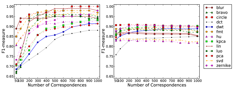
In Tab. IX, we report the per-method best thresholds, once determined from the plain copies (middle column), and once for the mixed clean and JPEG-compressed images (right column). The average value in the bottom row shows that the JPEG artifacts decrease the optimum value to almost .
To further demonstrate the sensitivity of to JPEG compression, we performed two further evaluation scenarios (see Tab. IX and Tab. IX). Tab. IX reports the scores on images without postprocessing. Tab. IX reports the scores on images with several different types of postprocessing. Both tables relate the performance of individually selected thresholds versus fixed thresholds. In Tab. IX, it can be seen that the individual selection of (middle column) leads to slightly worse performance than a globally fixed, high . Interestingly, Tab. IX shows results for the “combined transformations” variant in our evaluation of the main paper, i. e. global JPEG compression at quality level , and slight modifications on the copied region (rotation of , upsampling of ). Note that for this scenario, we did not conduct dedicated fine-tuning of . Nevertheless, the average for method-specific values of (Tab. IX middle) are by a large margin better than the fixed threshold for plain 1-to-1 copies. Our further performance analysis was based on the lower thresholds, as one of our goals is to evaluate the influence of postprocessing artifacts on the features.
One alternative would be to optimize for every experiment (e. g. Gaussian noise, or JPEG compression) separately. However, we considered such a complete threshold fine-tuning unrealistic. In practice, it is only expected that “some postprocessing” has been done to better fit a copied region in its environment. Thus, a successful CMFD algorithm must be able to deal with a certain amount of uncertainty on the actual type of postprocessing.
X Results with score
All plotted results in the main paper are presented using precision and recall. However, in some cases (like the determination of ), a single number is required to more easily compare feature sets. In the tables of the main paper, we added the score which subsumes precision and recall. For completeness, we add here the results of the remaining experiments from the main paper with respect to the score.
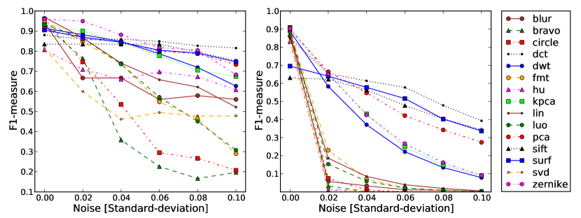
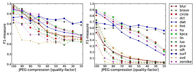
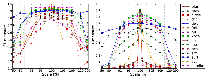
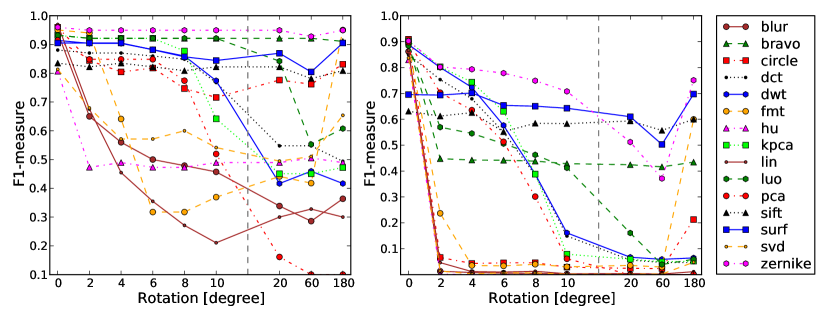
The plots in Fig. V-B1 correspond to the results shown in Fig. 8 and Fig. 9 in the main paper. The left plot shows the results at image level, while the right side shows the results for the same experiment at pixel level. The order of the experiments, and the experimental setup, is the same as in the main paper. Thus, from top to bottom, results are presented for additive Gaussian noise, varying degrees of JPEG compression, a limited amount of scaling, and varying degrees of rotation. We relate the scores to the precision and recall plots from the main paper. In general, the score captures large dynamics in precision and recall. For the Gaussian noise, the large spread in the recall mainly shapes both scores, at image level and pixel level. For the experiment on JPEG compression, the image level differences in precision and recall are evened out in the score. At pixel level, the large differences in recall again shape the score. The recall also mainly influences the scores on scaling and rotation.
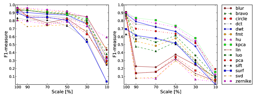
Fig. 16 shows the scores that correspond to Fig. 10 in the main paper. It shows the performance deterioriation under increasing downsampling. On the left side, we evaluated the performance at image level, on the right side at pixel level. The results of the score are again mostly influenced by the recall. Note that we omitted a performance evaluation at image level in the main paper, mainly to improve the flow of the presentation.
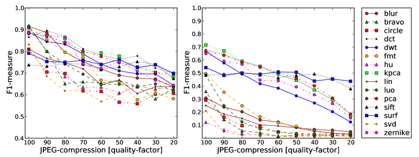
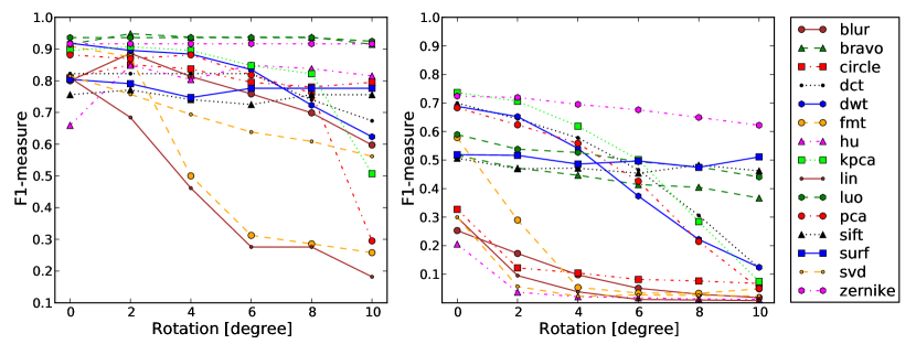
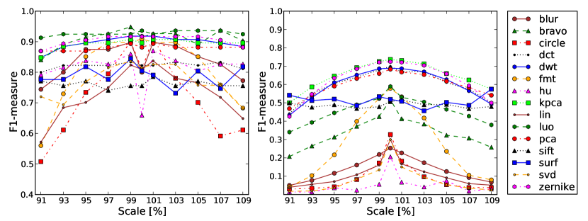
The scores for varios scenarios applied on the downsampled version of the images are shown in Fig. V-B1 (see Fig. 11 in the main paper). Again, on the left side, we show the performance at image level, on the right side at pixel level. From top to bottom, we present results on JPEG compression, rotation and scaling of the copied snippet. Again, in all three cases, recall mainly influences the score.
XI Postprocessing of Keypoint-based Methods
We apply a hierarchical clustering on matched feature pairs, i. e. assign each point to a cluster and merge them according to a linkage-method, as described by Amerini et al. [3]. For the linkage method we chose “single” linkage as it is very fast to compute and as the choice of the linkage-method is not critical [3]. On the other hand, the stop condition for merging the clusters (“cut-threshold”) plays an important role. Here, we did not use the inconsistency coefficient as proposed by Amerini et al.. Instead, we rely on the distance between the nearest clusters. Two clusters are merged if their distance lies within the cut-threshold. We chose to use a cut-threshold of pixels for SIFT and pixels for SURF. As a special case, if we obtained less than matches, the cut-threshold is raised to pixels. Note that the cut-thresholds are chosen in a defensive way, such that typically multiple smaller clusters remain, which are merged at a later stage of the algorithm.
If a minimum of correspondences connects two of these clusters, we estimate with RANSAC the affine transformation between the points that are connected by these correspondences, analogously to Amerini et al. [3]. In contrast to prior work, we further compute the optimal transformation matrix from the inliers according to the gold-standard algorithm for affine homography matrices [34, pp. 130]. Transformations with implausibly large or small values are removed via thresholding.
For large images containing large copied areas the transformation matrices of the clusters may often be similar. So, we decided to merge them if the root mean square error (RMSE) between two transformation matrices is below a threshold of for the scaling and rotation part of the matrix, and below a threshold of for the translation part. For these merged clusters we reestimate the transformation with the same procedure as above.
For each cluster we warp the image according to the estimated transformation matrix and compute a correlation map between the image and its warped version. From here on, we follow the algorithm by Pan and Lyu [22]. For every pixel and its warped version we compute the normalized correlation coefficient with a window size of pixels. To remove noise in the correlation map, it is smoothed with a pixels Gaussian kernel. Every smoothed correlation map is then binarized with a threshold of , and areas containing less than pixels were removed. Furthermore, areas where no match lies were removed, too. Then, the outer contours of each area is extracted and the inner part is flood-filled, which closes holes in the contours. The output map is the combination of all post-processed correlation maps. As a final verification step, each area from the combined output map is tested if it also has a correspondence which lies in another marked area.
XII Database Categories
In the main paper, we report results on the full dataset. However, the performance of the feature descriptors undoubtedly depends on the content of the image and the copied area. With a subdivision of the dataset in smaller categories, we make an attempt towards better explaining the performance differences of the feature sets.
The design of a proper category-driven evaluation in image forensics is still an open problem. We made a first attempt towards a proper categorization using two different approaches. We divided the images in multiple categories, once into object categories and once in texture categories. The results are reported in Sec. XII-A and Sec. XII-B, respectively.
XII-A Categorization by Object Classes
We split the images in categories where the copied regions belong to one of the object categories living, nature, man-made or mixed. Here, mixed denotes copies where arguably multiple object types occur. Table IX lists which image belongs to which category. In Sec. XIII, downsampled versions of the images are presented together with the names of the images. The number of images varies between the categories.
| Assigned images | ||
|---|---|---|
| Category | Small copied area | Large copied area |
| living | giraffe, jellyfish chaos, cattle, swan | four babies |
| nature | fisherman, no beach, berries, | Scotland, white, hedge, christmas hedge, Malawi, beach wood, tree |
| man-made | supermarket, bricks, statue, ship, sailing, dark and bright, sweets, disconnected shift, Egyptian, noise pattern, sails, mask, window, writing history, knight moves | horses, kore, extension, clean walls, tapestry, port, wood carvings, stone ghost, red tower |
| mixed | barrier, motorcycle, Mykene, threehundred, Japan tower, wading, central park | fountain, lone cat |
The smallest category is living containing test cases, the largest category is man-made ( test cases). Note that the varying category sizes pose no problem, as we only compute the performance within a category666For instance, for classification tasks, a balanced size of each category can prevent biased results. However, this is not of concern in our copy-move forgery evaluation.. We used the same parameters as for the evaluations in the main paper. Tab. XII-A shows the score for plain copy-move forgeries at image level (left) and at pixel level (right). Note that all four categories perform comparably at pixel level. However, at image level, most feature sets perform best for living and nature.
| Image level | Pixel level | |||
| Method | man-made | mixed | man-made | mixed |
| Blur | 96.00 | 97.30 | 65.64 | 64.40 |
| Bravo | 95.05 | 94.74 | 65.00 | 59.59 |
| Circle | 97.96 | 94.74 | 71.62 | 68.91 |
| DCT | 89.72 | 90.00 | 68.82 | 58.86 |
| DWT | 89.72 | 87.80 | 68.42 | 66.64 |
| FMT | 95.05 | 94.74 | 69.95 | 67.98 |
| Hu | 86.49 | 76.60 | 64.89 | 61.50 |
| KPCA | 91.43 | 92.31 | 70.56 | 70.37 |
| Lin | 97.96 | 97.30 | 69.57 | 66.11 |
| Luo | 96.00 | 94.74 | 65.03 | 59.59 |
| PCA | 89.72 | 94.74 | 69.88 | 69.35 |
| Sift | 88.00 | 88.89 | 71.87 | 69.26 |
| Surf | 90.20 | 94.12 | 75.97 | 66.71 |
| SVD | 85.71 | 78.26 | 68.71 | 60.49 |
| Zernike | 95.05 | 100.00 | 71.04 | 68.00 |
| Average | 92.27 | 91.75 | 69.13 | 65.18 |
The Figures V-B1, V-B1, V-B1 and V-B1 show the results for living, nature, man-made and mixed under Gaussian noise, JPEG compression, rotation, scaling and joint effects. Again, the evaluation parameters were the same as in the main paper. At pixel level, several feature sets perform better for nature than for living. However, in several scenarios, the best results are obtained in the categories man-made and mixed. We assume that this comes from the fact that man-made objects often exhibit a clearer structure, and as such encompass the task of copy-move forgery detection.
![[Uncaptioned image]](/html/1208.3665/assets/x26.png)
![[Uncaptioned image]](/html/1208.3665/assets/x27.png)
![[Uncaptioned image]](/html/1208.3665/assets/x28.png)
![[Uncaptioned image]](/html/1208.3665/assets/x29.png)
![[Uncaptioned image]](/html/1208.3665/assets/x30.png)
![[Uncaptioned image]](/html/1208.3665/assets/x31.png)
![[Uncaptioned image]](/html/1208.3665/assets/x32.png)
![[Uncaptioned image]](/html/1208.3665/assets/x33.png)
![[Uncaptioned image]](/html/1208.3665/assets/x34.png)
![[Uncaptioned image]](/html/1208.3665/assets/x35.png)
![[Uncaptioned image]](/html/1208.3665/assets/x36.png)
![[Uncaptioned image]](/html/1208.3665/assets/x37.png)
![[Uncaptioned image]](/html/1208.3665/assets/x38.png)
![[Uncaptioned image]](/html/1208.3665/assets/x39.png)
![[Uncaptioned image]](/html/1208.3665/assets/x40.png)
![[Uncaptioned image]](/html/1208.3665/assets/x41.png)
![[Uncaptioned image]](/html/1208.3665/assets/x42.png)
![[Uncaptioned image]](/html/1208.3665/assets/x43.png)
![[Uncaptioned image]](/html/1208.3665/assets/x44.png)
![[Uncaptioned image]](/html/1208.3665/assets/x45.png)
XII-B Categorization by Texture
We investigated a second categorization of the dataset, this time by texture. The dataset is divided in copied areas providing smooth, rough and structured content. Here, smooth and rough serves as a distinction of texture properties, which can be approximately seen as low or high entropy in the snippet. The third category, structured, refers in most cases to man-made structures, like buildings: regular, clearly pronounced edges and corners.
This categorization was already prepared during the creation of the dataset. We aimed to use a diverse set of scenes, providing various challenges to the detectors. One challenge of real-world forgeries is the fact that we have little control over the creation of the manipulation. As a consequence, the texture categories are not based on quantitative measures. Instead, we used the artists’ result on a fuzzy task description, like to “create a copy with little texture”. Given the fact that real-world copy-move forgeries are done from artists as well, we found it reasonable to adopt the artists’ viewpoint on CMFD.
Tab. XI shows the assignment of images to categories. For our evaluation, we did not distinguish the size of the copied areas. Thus, we compare the three major categories smooth, rough and structured. The number of motifs per category is , and , respectively.
| Assigned images | ||
|---|---|---|
| Category | Small copied area | Large copied area |
| Smooth | ship, motorcycle, sailing, disconnected shift, noise pattern, berries, sails, mask, cattle, swan, Japan tower, wading | four babies, Scotland, hedge, tapestry, Malawi |
| Rough | supermarket, no beach, fisherman, barrier, threehundred, writing history, central park | lone cat, kore, white, clean walls, tree, christmas hedge, stone ghost, beach wood, red tower |
| Structured | bricks, statue, giraffe, dark and bright, sweets, Mykene, jellyfish chaos, Egyptian, window, knight moves | fountain, horses, port, wood carvings, extension |
Tab. XII-B, Fig. V-B1, Fig. V-B1 and Fig. V-B1 show the results per category. On the left side, the results are shown at image level, on the right side at pixel level. The most notable performance shift across categories is the relation between keypoint- and block-based methods. Surf and Sift perform best in rough (see Fig. V-B1), while block-based methods often have an advantage in smooth (see Fig. V-B1). In the category structure (see Fig. V-B1), block-based and keypoint-based methods perform similarly well.
![[Uncaptioned image]](/html/1208.3665/assets/x46.png)
![[Uncaptioned image]](/html/1208.3665/assets/x47.png)
![[Uncaptioned image]](/html/1208.3665/assets/x48.png)
![[Uncaptioned image]](/html/1208.3665/assets/x49.png)
![[Uncaptioned image]](/html/1208.3665/assets/x50.png)
![[Uncaptioned image]](/html/1208.3665/assets/x51.png)
![[Uncaptioned image]](/html/1208.3665/assets/x52.png)
![[Uncaptioned image]](/html/1208.3665/assets/x53.png)
![[Uncaptioned image]](/html/1208.3665/assets/x54.png)
![[Uncaptioned image]](/html/1208.3665/assets/x55.png)
![[Uncaptioned image]](/html/1208.3665/assets/x56.png)
![[Uncaptioned image]](/html/1208.3665/assets/x57.png)
![[Uncaptioned image]](/html/1208.3665/assets/x58.png)
![[Uncaptioned image]](/html/1208.3665/assets/x59.png)
![[Uncaptioned image]](/html/1208.3665/assets/x60.png)
XIII Overview on the Forgery Database
We comment on the implementation of the benchmarking framework, with emphasis on its extensibility. Then, we briefly discuss the choice of the manipulated regions. Finally, we show all reference manipulations of the database, and their associated ground truth.
Recall that the database consists of base images and prepared image regions from these images, called snippets. Base images and snippets are spliced, to simulate a close-to-real-world copy-move forgery. During splicing, postprocessing artifacts can be added to the snippets and the final output images. The software to create tampered images and the associated ground truth is written in C++ and is best used with scripts written in Perl. Within the Perl-scripts, a series of output images can be created by iterating over a parameter space. For instance, all spliced images with JPEG compression are obtained by iterating over the JPEG quality parameter space. We call one such parameterization a configuration. Upon acceptance of the paper, all images, snippets, code, scripts and configuration files are made publicly available from our web page. Note that with the separate building blocks, it is straightforward to add a copy-move tampering scenario that has not been addressed so far. For instance, assume (hypothetically) that one aims to evaluate instead of Gaussian noise Laplacian noise on the inserted regions. Then, all that is required from the author is to add a Laplacian noise function to the C++ code, and to add a matching configuration to the perl scripts.
Fig. 25, Fig. 26 and Fig. 27 show a preview of the images and the regions of plain copy-move forgeries, sorted by the categories smooth, rough and structure. For every tampering example we show at the top the image containing the “reference” tampered regions. At the bottom we show the associated ground truth (with white being the copy-source or copy-target regions). Note that several aspects vary over the images, e. g. the size of the copied regions, or the level of detail in the copied region. Note also, that the assignment of categories is debatable. For instance, in Fig. 27 the jellyfish image (top row, third image). Upon close examination, the jellyfish exhibit pronounced edges, although it is not a man-made structure. As presented, the copied regions are meaningful, i. e. either they hide image content, or they emphasize an element of the picture. Note, however, that the software allows the snippets to be inserted at arbitrary positions. Thus, one could equally well create semantically meaningless forgeries. This is often the case when the copied region is rotated and resampled. In such cases, the image content becomes (naturally) implausible.


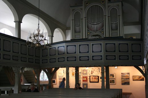

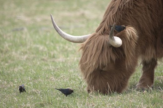

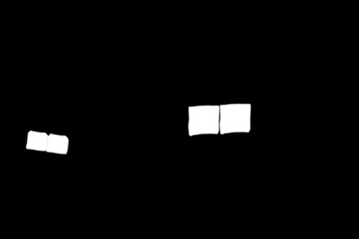
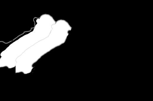
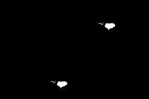




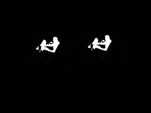
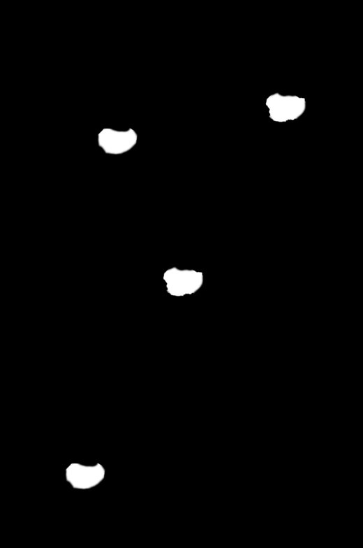
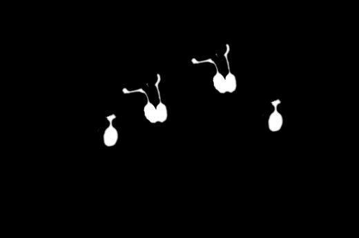



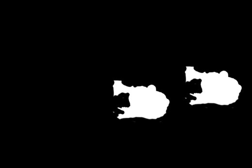
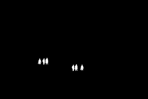


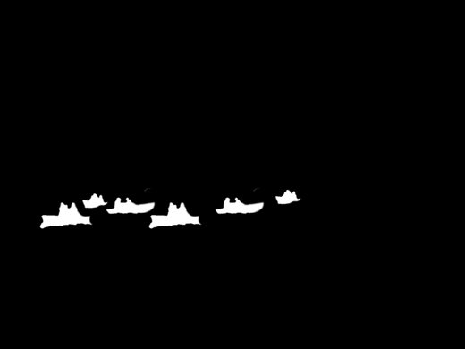
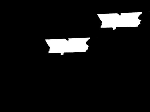
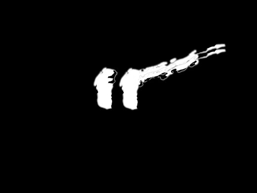



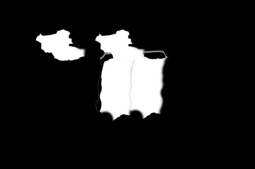
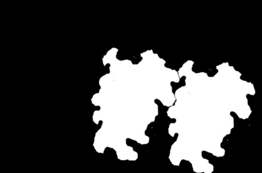

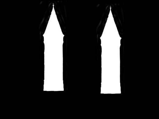
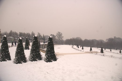

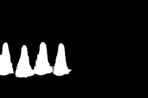
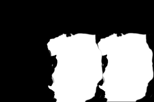
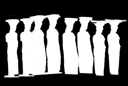
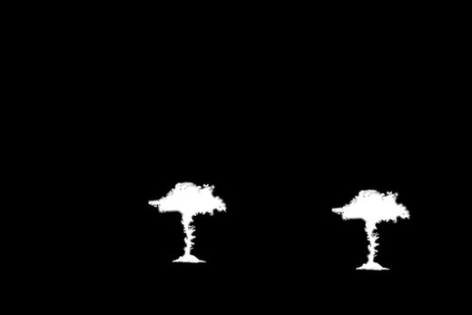

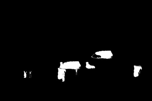

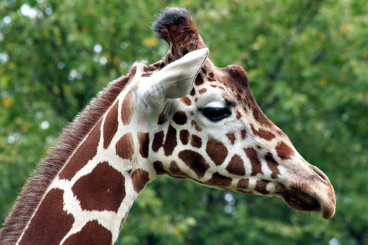
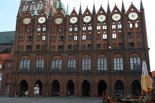
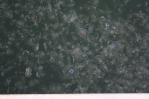
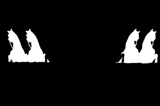

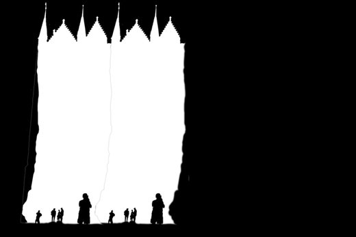
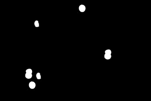
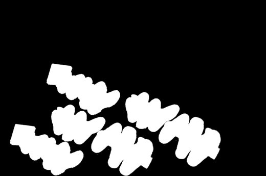

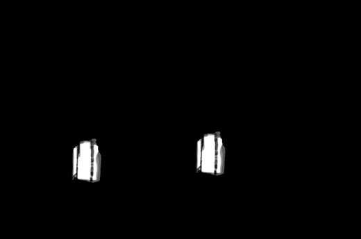

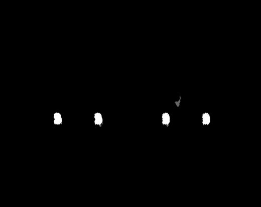


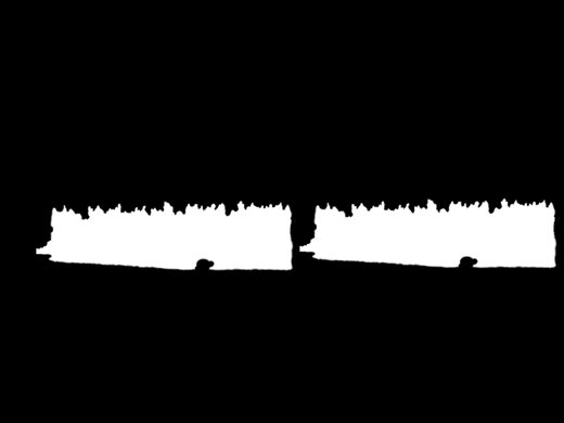
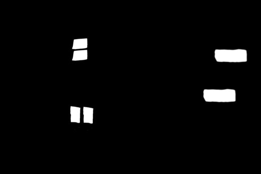

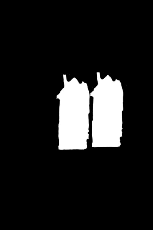
![[Uncaptioned image]](/html/1208.3665/assets/images/authors/vince.jpg) |
Vincent Christlein received his Diploma degree in computer science in 2012 from the University of Erlangen-Nuremberg, Germany. During winter 2010, he was a visiting research student at the Computational Biomedicine Lab, University of Houston, USA. Currently, he is a doctoral student at the Pattern Recognition Lab, University of Erlangen-Nuremberg. His research interests lie in the field of computer vision and computer graphics, particularly in image forensics, reflectance modeling, and historical document analysis. |
![[Uncaptioned image]](/html/1208.3665/assets/images/authors/chris.jpg) |
Christian Riess received his Diploma degree in computer science in 2007 from the University of Erlangen-Nuremberg, Germany. He was working on an industry project with Giesecke+Devrient on optical inspection from 2007 to 2010. He is currently pursuing a Ph.D. degree at the Pattern Recognition Lab, at the University of Erlangen-Nuremberg, Germany. His research interests include computer vision and image processing and in particular illumination and reflectance analysis and image forensics. |
![[Uncaptioned image]](/html/1208.3665/assets/images/authors/johannes.jpg) |
Johannes Jordan received his Diploma degree in computer science in 2009 from the University of Erlangen-Nuremberg, Germany. He was a visiting scholar at Stony Brook University, Stony Brook, NY, in 2008. Currently, he is pursuing a Ph.D. degree at the Pattern Recognition Lab, University of Erlangen-Nuremberg, Germany. His research interests focus on computer vision and image processing, particularly in reflectance analysis, multispectral image analysis and image forensics. |
![[Uncaptioned image]](/html/1208.3665/assets/images/authors/corinna.jpg) |
Corinna Riess received her Diploma degree in social sciences in 2011 from the University of Erlangen-Nuremberg, Germany. She is currently working as online marketing manager and web developer for xeomed, Nuremberg, Germany. Her further interests include print media layout and image processing and editing. |
![[Uncaptioned image]](/html/1208.3665/assets/images/authors/Elli.jpg) |
Elli Angelopoulou received her Ph.D. in Computer Science from the Johns Hopkins University in 1997. She did her postdoc at the General Robotics, Automation, Sensing and Perception (GRASP) Laboratory at the University of Pennsylvania. She then became an assistant professor at Stevens Institute of Technology. She is currently an associate research professor at the University of Erlangen-Nuremberg. Her research focuses on multispectral imaging, skin reflectance, reflectance analysis in support of shape recovery, image forensics, image retrieval and reflectance analysis in medical imaging (e.g. capsule endoscopy). She has over 50 publications, multiple patents and has received numerous grants, including an NSF CAREER award. Dr. Angelopoulou has served on the program committees of ICCV, CVPR and ECCV and is an associate editor of Machine Vision and Applications (MVA) and the Journal of Intelligent Service Robotics (JISR). |