Discussion of “Statistical Modeling of Spatial Extremes” by A. C. Davison, S. A. Padoan and M. Ribatet

10.1214/11-STS376

, , and

We congratulate the authors for producing such a helpful and comprehensive overview paper of a rapidly developing and important area. The starting point for inference in spatial extreme value problems is to identify which features of the process require modeling. In certain applications, for example, in the generation of return period maps, only the marginal behavior is of concern. For such applications, the covariate hierarchical/latent variable models reviewed in Section 4 are ideal. However, if there is any dependence in the process between sites, then care needs to be taken when assessing the uncertainty in the estimated marginal distribution; the composite likelihood procedures detailed in Section 6.2 can also be exploited in this context when one wishes to avoid assumptions on the form of the spatial dependence. As the authors point out, however, if interest lies in modeling the joint occurrence of extremes over a region, then the dependence structure of the spatial process needs to be explicitly modeled. The most widely used approach in such cases is to model the process as a max-stable process. Here we will explore the suitability of this framework for modeling spatial extremes, since these processes are quite restrictive in their assumptions. Specifically, all finite dimensional distributions of a max-stable process are multivariate extreme distributions. Even simply in the bivariate case, this corresponds to the variables being exactly independent or asymptotically dependent. Consequently, the broad class of asymptotically independent variables is precluded under the modeling assumptions of max-stable processes.

First consider diagnostic testing for the process being max-stable. From our experience we feel that in many applications, max-stable processes are assumed to be appropriate without testing their suitability for the data. A partial justification for this is that often it is pointwise maxima that are being modeled, and so just as one appeals to the marginal limit theory to justify fitting the GEV distribution site-wise, it seems natural to appeal to the limit theory for the dependence structure also. However, we would typically not fit the GEV to the margins blindly, but look to assess its suitability through diagnostics such as Q-Q plots. To our knowledge, there currently are no diagnostics for testing if the process is max-stable, and so this discussion contribution aims to provide such a test.

Suppose that $\{Y(\mathbf{x})\dvtx\mathbf{x}\in A\}$ is a max-stable process on the region $A$ with standard Gumbel marginal distributions for all $\mathbf{x}$. This is simply attained through a pointwise log transformation of the more commonly-assumed standard Fréchet margins. As the process will typically only be observed at a finite set of sites $\mathbf{x}_{1},\ldots,\mathbf{x}_{m}$, then all that can be tested for in practice is that the joint distribution of $\{Y(\mathbf{x}_{j})\dvtx\break j\in\Delta\}$, where $\Delta=\{1,\ldots,m\}$, follows a multivariate extreme value distribution. Then for any $D\subseteq\Delta$ we have that the joint distribution function for $\{Y(\mathbf{x}_{j})\dvtx\break j\in D\}$ is

$$G_{D}(\mathbf{y})=\exp[-V_{D}\{\exp(\mathbf{y})\}],$$

where $V_{D}$ is the associated exponent measure; see Section 2.3. A key property of $G_{D}$, due to max-stability, is that the distribution of $Y_{D}=\max_{j\in D}Y(\mathbf{x}_{j})$ is

$$H_{D}(y)=G_{D}(y\mathbf{1})=\exp[-\exp\{-(y-\mu_{D})\}].$$

This is a Gumbel distribution with location parameter $\mu_{D}=\log V_{D}(\mathbf{1})$ where $0\leq\mu_{D}\leq\log(|D|)$, due to bounds on the exponent measure. It follows that $Z_{D}=Y_{D}-\mu_{D}$ is standard Gumbel for all $D\subseteq\Delta$. The idea of the diagnostic is to pool values of $Z_{D}$ over replicates of the max-stable process and over all $D\subseteq\Delta$, of a particular cardinality $k=|D|$, and test using a P-P plot whether the variables $Z_{D}$ follow a standard Gumbel distribution. This enables an assessment of the $k$th dimensional properties of the process. Here we look at $k=2,3,4,m$.

There are a few practical issues to address. As the value of $\mu_{D}$ is unknown for all $D$ with $|D|\geq 2$, these parameters require estimation. We used maximum likelihood to estimate $\mu_{D}$, based upon replicate data for $Y_{D}$, and subject to the parameter constraints above; this was found to give better estimates than moment methods. There are ${m\choose|D|}$ sets with size $|D|$ in the power set of $\Delta$, thus, for $m$ large, it is computationally intensive to determine an estimate for all possible $\mu_{D}$. As a result, we limit ourselves to a randomly selected sample of 500 possibilities for $D$ with $|D|=k$. Although we did not explore this choice in more detail, it would seem reasonable not to examine subsets $D$ in which the included sites are likely to be independent, since the ability to detect a departure from max-stability will be limited in these cases. In order to determine the variability of our estimates, we use a nonparametric bootstrap to produce 95$\%$ confidence intervals. Bootstrap methods are required as there is clearly dependence in the pooled data over different $D$. By treating each replicate of the process as a block, and constructing $Z_{D}$ through estimation of $\mu_{D}$ for each bootstrap sample, this complicated dependence is naturally incorporated into the confidence intervals.

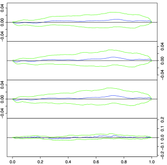
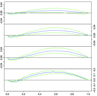
Three different simulated data sets were used to illustrate the methods, with 1000 replicates of the variables generated on a regular grid of sites over a $10\times 10$ unit square. The different dependence structures used were as follows: a Smith model max-stable process (with identity covariance matrix $\Omega$); a multivariate extreme value distribution with logistic dependence structure (dependence parameter $\alpha=0.7$); and a Gaussian process with exponential correlation function ($\lambda=0.7^{-1}$), pointwise trans-formed to have standard Gumbel marginal distributions. The first two examples are max-stable in their dependence structure, that is, follow multivariate extreme value distributions at the sites on the grid. The third example, having a Gaussian copula, is not max-stable.

Figure 1: Rescaled P-P plot for $Z_{D}$ derived from the Smith max-stable process model. Top–bottom: $|D|=2,3,4,100$.

Figure 2: As Figure 1, but for the multivariate logistic distribution.

Figures 1–3 show the diagnostic P-P plots for the three dependence structures respectively. Each figure illustrates the diagnostic for $k=2,3,4,100$, with the P-P plot presented on the $y$-axis as a difference between the empirical and model probabilities. For the first two processes the horizontal line, representing no departure from the model probability, falls inside the pointwise 95% confidence intervals, thus indicating that the data provide no evidence against a max-stable model. This is not the case for the Gaussian process copula, which produces evidence to reject max-stability for each value of $k$. Interestingly, the power of the test increases with $k$ (note the change of scale on the bottom subplot). If only the $k=2$ case had been used with a smaller sample size or weaker dependence we would wrongly have failed to reject the null for the Gaussian copula. This indicates that higher order dependence plays an important role in identifying the nature of the extremal dependence. Currently, however, the standard methods to fit max-stable processes use only the bivariate distributions, through composite likelihood methods, as detailed in Section 6.2.

Figure 3: As Figure 1, but for the Gaussian copula.

More generally, this highlights that pairwise modeling techniques may not always be as effective as one would hope. Even if the process has bivariate extreme value pairwise distributions, this does not ensure that higher order distributions are max-stable, or even asymptotically dependent. The restriction to pairwise likelihood is to a large part due to intractability of higher order distributions of max-stable processes. As noted by the authors, higher order distributions for the Smith model can be expressed (Genton, Ma and Sang (2011)), though the model’s utility is limited due to its unrealistic process realizations. In terms of the copula models of Section 5, Nikoloulopoulos, Joe and Li (2009) provide the $d$-dimensional copulas for the extremal $t$ and, through the appropriate limits, the Hüsler–Reiss analogue. The authors comment on the intriguing links between the copula and process models. It would seem to us that the extremal $t$ copula has the immediate interpretation as the limiting finite-dimensional dependence structure of normalized spatial $t$ processes. Kabluchko, Schlather and de Haan (2009) similarly demonstrate that the Brown–Resnick, analogous to the Hüsler–Reiss, limit arises from normalized maxima of Gaussian processes which become increasingly dependent through contraction of the spatial domain at an appropriate rate. Consequently, these two copula models could equally be viewed as max-stable process models. We thus agree with the authors’ suggestion that the connection is indeed a matter of extending the copula to the full spatial domain. Evidently, the utility of full spatial process models lies in being able to assess features at unobserved sites; this is aided in the current context by simulation of the full process. For the extremal $t$ model, the definition-based method described in Section 7.1 and illustrated in Figure 7 seems adequate for this. The alternative would be to derive the appropriate spectral process $W(\mathbf{x})$ and exploit representation (20), though it is not clear that this would be simpler. For the Hüsler–Reiss extension, it appears that correspondence with Brown–Resnick processes would permit simulation, through the methods already employed in the paper.

At a more conceptual level, the major restriction of max-stable processes is that the form of the extremal dependence at observed levels must be assumed to hold for all more extreme events. However, it may often seem more plausible that the dependence could weaken at extreme levels, with the largest extremes becoming more isolated as energy is concentrated into a more localized area. While max-stable process models may well be sufficiently flexible to describe observed extremal dependence, for the purposes of extrapolation we would really like to be sure that the assumed stability holds. This can also be examined through the empirical decay of tail probabilities. Suppose $X(\mathbf{x})$ represents the original data process (before taking pointwise maxima), but transformed to have common Gumbel margins. Define $\bar{F}_{D}(x\mathbf{1})=\Pr\{X(\mathbf{x}_{i})>x\dvtx i\in D\}$; if the dependence structure is asymptotically dependent, then $\bar{F}_{D}(x\mathbf{1})=O\{\exp(-x)\}$ as $x\rightarrow\infty$. If this feature is observed in the data, this suggests that the limiting max-stable process is different from independence, and extrapolations based upon fitting these processes may be reliable. If asymptotic independence is present in the data, $\bar{F}_{D}(x\mathbf{1})=O\{\exp(-x/\break\eta_{D})\}$, for some $\eta_{D}\in(0,1)$. If this feature is observed in the data, then we would be rightfully skeptical that fitting a max-stable process would provide reliable extrapolations. Some recent work by Wadsworth and Tawn (2012) explores the extremal properties of a class of spatial processes which satisfy this property.

References

- Genton, Ma and Sang (2011) {barticle}[mr] \bauthor\bsnmGenton, \bfnmMarc G.\binitsM. G., \bauthor\bsnmMa, \bfnmYanyuan\binitsY. and \bauthor\bsnmSang, \bfnmHuiyan\binitsH. (\byear2011). \btitleOn the likelihood function of Gaussian max-stable processes. \bjournalBiometrika \bvolume98 \bpages481–488. \biddoi=10.1093/biomet/asr020, issn=0006-3444, mr=2806443 \bptokimsref \endbibitem
- Kabluchko, Schlather and de Haan (2009) {barticle}[mr] \bauthor\bsnmKabluchko, \bfnmZakhar\binitsZ., \bauthor\bsnmSchlather, \bfnmMartin\binitsM. and \bauthor\bparticlede \bsnmHaan, \bfnmLaurens\binitsL. (\byear2009). \btitleStationary max-stable fields associated to negative definite functions. \bjournalAnn. Probab. \bvolume37 \bpages2042–2065. \biddoi=10.1214/09-AOP455, issn=0091-1798, mr=2561440 \bptokimsref \endbibitem
- Nikoloulopoulos, Joe and Li (2009) {barticle}[mr] \bauthor\bsnmNikoloulopoulos, \bfnmAristidis K.\binitsA. K., \bauthor\bsnmJoe, \bfnmHarry\binitsH. and \bauthor\bsnmLi, \bfnmHaijun\binitsH. (\byear2009). \btitleExtreme value properties of multivariate copulas. \bjournalExtremes \bvolume12 \bpages129–148. \biddoi=10.1007/s10687-008-0072-4, issn=1386-1999, mr=2515644 \bptokimsref \endbibitem
- Wadsworth and Tawn (2012) {bmisc}[auto:STB—2012/03/21—07:41:58] \bauthor\bsnmWadsworth, \bfnmJ. L.\binitsJ. L. and \bauthor\bsnmTawn, \bfnmJ. A.\binitsJ. A. (\byear2012). \bhowpublishedDependence modelling for spatial extremes. Biometrika. To appear. DOI:\doiurl10.1093/biomet/asr080. \bptokimsref \endbibitem