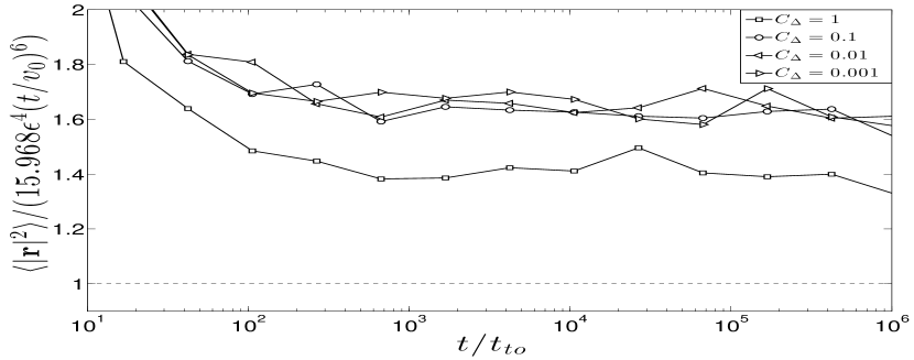
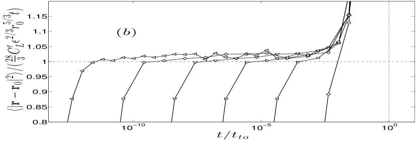
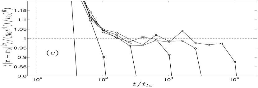
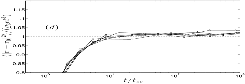
Do Sweeping Effects Suppress Particle Dispersion in Synthetic Turbulence?

Gregory L. Eyink1,212{\,\!}^{1,2} eyink@jhu.edu    Damien Benveniste22{\,\!}^{2} 11{\,\!}^{1}Department of Applied Mathematics & Statistics
and 22{\,\!}^{2}Department of Physics & Astronomy
The Johns Hopkins University, USA
Abstract

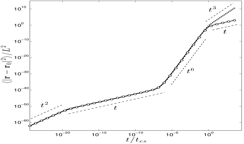
Synthetic models of Eulerian turbulence like so called “Kinematic Simulations” (KS) are often used as computational shortcuts for studying Lagrangian properties of turbulence. These models have been criticized by Thomson & Devenish (2005), who argued on physical grounds that sweeping decorrelation effects suppress pair dispersion in such models. We derive analytical results for Eulerian turbulence modeled by Gaussian random fields, in particular for the case with zero mean velocity. Our starting point is an exact integrodifferential equation for the particle pair separation distribution obtained from the Gaussian integration-by-parts identity. When memory times of particle locations are short, a Markovian approximation leads to a Richardson-type diffusion model. We obtain a time-dependent pair diffusivity tensor of the form Kij(𝐫,t)=Sij(𝐫)τ(r,t)subscript𝐾𝑖𝑗𝐫𝑡subscript𝑆𝑖𝑗𝐫𝜏𝑟𝑡K_{ij}({\bf r},t)=S_{ij}({\bf r})\tau(r,t) where Sij(𝐫)subscript𝑆𝑖𝑗𝐫S_{ij}({\bf r}) is the structure-function tensor and τ(r,t)𝜏𝑟𝑡\tau(r,t) is an effective correlation time of velocity increments. Crucially, this is found to be the minimum value of three times: the intrinsic turnover time τeddy(r)subscript𝜏𝑒𝑑𝑑𝑦𝑟\tau_{eddy}(r) at separation r𝑟r, the overall evolution time t,𝑡t, and the sweeping time r/v0𝑟subscript𝑣0r/v_{0} with v0subscript𝑣0v_{0} the rms velocity. We study the diffusion model numerically by a Monte Carlo method. With moderate inertial-ranges like those achieved in current KS, our model is found to reproduce the t9/2superscript𝑡92t^{9/2} power-law for pair dispersion predicted by Thomson & Devenish and observed in the KS. However, for much longer ranges, our model exhibits three distinct pair-dispersion laws in the inertial-range: a Batchelor t2superscript𝑡2t^{2}-regime, followed by a Kraichnan-model-like t1superscript𝑡1t^{1} diffusive regime, and then a t6superscript𝑡6t^{6} regime. Finally, outside the inertial-range, there is another t1superscript𝑡1t^{1} regime with particles undergoing independent Taylor diffusion. These scalings are exactly the same as those predicted by Thomson & Devenish for KS with large mean velocities, which we argue hold also for KS with zero mean velocity. Our results support the basic conclusion of Thomson & Devenish (2005) that sweeping effects make Lagrangian properties of KS fundamentally different from hydrodynamic turbulence for very extended inertial-ranges.

pacs:
47.27.Ak, 47.27.tb, 47.27.eb, 47.27.E-

I Introduction

How particle pairs separate in a turbulent flow has been a central subject of turbulence research since the classical work of Richardson Richardson (1926). Unfortunately, the phenomenon has proved quite difficult to investigate by numerical solution of the fluid equations and by controlled laboratory experiments, especially because of the very large Reynolds numbers required. Many studies have therefore employed “synthetic turbulence” or ensembles of random velocity fields with some of the scaling properties of real turbulent velocities but which can be efficiently sampled even for very long scaling ranges. For example, papers Elliott, Jr. and Majda (1996); Fung and Vassilicos (1998); Malik and Vassilicos (1999); Dávila and Vassilicos (2003); Nicolleau and Yu (2004) have followed this approach and have reported substantial agreement of their numerical simulations with the predictions of Richardson, including the famous “t3superscript𝑡3t^{3}-law” for the growth in time of mean square pair separation distances.

The validity of these results has been called into question, however. A paper of Chaves et al. Chaves et al. (2003) pointed out that the use of synthetic turbulence to model Eulerian velocity statistics implies sweeping effects of large-scale eddies on particle motions that diverge with the Reynolds number. Those authors suggested to employ synthetic ensembles such as Gaussian random fields to model instead the turbulent statistics of Lagrangian velocities. In a simple one-dimensional Gaussian model of Eulerian velocities they found analytically that large-scale sweeping effects “localized” particle pairs and prevented them from separating. Subsequently, in a very interesting paper Thomson and Devenish (2005), Thomson & Devenish have proposed an intuitive picture how sweeping affects particle dispersion in synthetic models of Eulerian turbulence. The key point is that large-scale eddies in real turbulence advect both particles and smaller scale eddies, while large-scale eddies in synthetic turbulence advect only particle pairs and not smaller eddies. This fact implies that particle pairs at separations r𝑟r in synthetic turbulence should experience rapidly changing relative velocities, as they are swept into new, statistically independent eddies. This occurs on a “sweeping” time-scale τsw(r)r/v0,similar-tosubscript𝜏𝑠𝑤𝑟𝑟subscript𝑣0\tau_{sw}(r)\sim r/v_{0}, where v0subscript𝑣0v_{0} is the rms velocity set by the largest eddies in the synthetic ensemble. Thomson & Devenish assume a diffusion process of pair separations with an eddy-diffusivity K(r)δu2(r)τsw(r)similar-to𝐾𝑟𝛿superscript𝑢2𝑟subscript𝜏𝑠𝑤𝑟K(r)\sim\delta u^{2}(r)\tau_{sw}(r) and δu2(r)𝛿superscript𝑢2𝑟\delta u^{2}(r) the mean-square relative velocity at separation r.𝑟r. In an ensemble with Kolmogorov scaling δu2(r)(εr)2/3,similar-to𝛿superscript𝑢2𝑟superscript𝜀𝑟23\delta u^{2}(r)\sim(\varepsilon r)^{2/3}, this yields dr2/dtK(r)ε2/3r5/3/v0similar-to𝑑superscript𝑟2𝑑𝑡𝐾𝑟similar-tosuperscript𝜀23superscript𝑟53subscript𝑣0dr^{2}/dt\sim K(r)\sim\varepsilon^{2/3}r^{5/3}/v_{0} and the solution

r2(t)ε4t6v06.similar-todelimited-⟨⟩superscript𝑟2𝑡superscript𝜀4superscript𝑡6superscriptsubscript𝑣06\langle r^{2}(t)\rangle\sim\frac{\varepsilon^{4}t^{6}}{v_{0}^{6}}. (1)

Note that this implies considerably slower growth than Richardson’s t3superscript𝑡3t^{3}-law 111The two laws can be written as <r2(t)>RichL2(t/tL)3similar-tosubscriptexpectationsuperscript𝑟2𝑡Richsuperscript𝐿2superscript𝑡subscript𝑡𝐿3<\!\!r^{2}(t)\!\!>_{{\rm Rich}}\sim L^{2}(t/t_{L})^{3} and <r2(t)>TDL2(t/tL)6similar-tosubscriptexpectationsuperscript𝑟2𝑡TDsuperscript𝐿2superscript𝑡subscript𝑡𝐿6<\!\!r^{2}(t)\!\!>_{{\rm TD}}\sim L^{2}(t/t_{L})^{6} in terms of the velocity integral scale L𝐿L and the large-eddy turnover time tLL/v0,similar-tosubscript𝑡𝐿𝐿subscript𝑣0t_{L}\sim L/v_{0}, by using εv03/L.similar-to𝜀superscriptsubscript𝑣03𝐿\varepsilon\sim v_{0}^{3}/L. In their regime of validity t<tL,𝑡subscript𝑡𝐿t<t_{L}, one has <r2(t)>TD<r2(t)>Rich.much-less-thansubscriptexpectationsuperscript𝑟2𝑡TDsubscriptexpectationsuperscript𝑟2𝑡Rich<\!\!r^{2}(t)\!\!>_{{\rm TD}}\,\,\ll\,\,<\!\!r^{2}(t)\!\!>_{{\rm Rich}}.. Thomson & Devenish argued for the above prediction in the case of a large mean sweeping, with v0subscript𝑣0v_{0} replaced by the mean speed u¯.¯𝑢\overline{u}. In the case of a zero-mean velocity ensemble, they argued instead for a t9/2superscript𝑡92t^{9/2}-growth law, intermediate between t3superscript𝑡3t^{3} and t6superscript𝑡6t^{6} (see our section III below). These predictions were supported in Thomson and Devenish (2005) by the numerical technique of “Kinematic Simulations” (KS) Elliott, Jr. and Majda (1996); Fung and Vassilicos (1998); Malik and Vassilicos (1999); Dávila and Vassilicos (2003); Nicolleau and Yu (2004). The previous contrary numerical results were explained on various grounds, e.g. the use of an adaptive time-stepping scheme in Elliott, Jr. and Majda (1996) which did not resolve the small sweeping time τsw(r)subscript𝜏𝑠𝑤𝑟\tau_{sw}(r) and its effect on particle dispersion.

The issues raised by the paper of Thomson & Devenish have still not been fully resolved. The numerical simulations in Thomson and Devenish (2005) used another form of adaptive time-stepping, which was suggested in Osborne et al. (2006) to be responsible for the observation of a t9/2superscript𝑡92t^{9/2} growth. Thomson & Devenish then repeated their simulations with a fixed small time-step and reported the same t9/2superscript𝑡92t^{9/2} law Devenish and Thomson (2009). The most recent simulations of Nicolleau & Nowakowski Nicolleau and Nowakowski (2011) for their longest scaling ranges show some evidence of the Thomson-Devenish sweeping effects, but the reported scaling laws are intermediate between those of Richardson and of Thomson-Devenish and agree with neither theory. Thus, there is still considerable uncertainty in the literature regarding the validity of the Thomson-Devenish theory. The question is important, because synthetic turbulence is a useful testing ground for numerical and theoretical methods, and because comparison of particle dispersion in synthetic and real turbulence illuminates the physical mechanisms of the latter.

Because of the disagreement of the numerical simulations of different groups, it is useful to have analytic results. The Thomson-Devenish arguments apply to a wide array of synthetic turbulence models, but Gaussian velocity ensembles are the most mathematically tractable. We therefore consider here the use of Gaussian random fields as models of turbulent Eulerian velocities. More precisely, we take the advecting velocity field 𝐮(𝐱,t)𝐮𝐱𝑡{\bf u}({\bf x},t) to be a Gaussian random field with mean 𝐮¯(𝐱,t)¯𝐮𝐱𝑡\overline{{\bf u}}({\bf x},t) and covariance Cij(𝐱,t;𝐲,s)=ui(𝐱,t)uj(𝐲,s)subscript𝐶𝑖𝑗𝐱𝑡𝐲𝑠delimited-⟨⟩superscriptsubscript𝑢𝑖𝐱𝑡superscriptsubscript𝑢𝑗𝐲𝑠C_{ij}({\bf x},t;{\bf y},s)=\langle u_{i}^{\prime}({\bf x},t)u_{j}^{\prime}({\bf y},s)\rangle for the fluctuations 𝐮=𝐮𝐮¯.superscript𝐮𝐮¯𝐮{\bf u}^{\prime}={\bf u}-\overline{{\bf u}}. Specific models of interest are similar to those studied in Chaves et al. (2003), with 𝐮¯(𝐱,t)=𝐮¯¯𝐮𝐱𝑡¯𝐮\overline{{\bf u}}({\bf x},t)=\overline{{\bf u}} independent of space and time and with covariance defined for 0<α<2,0<β<2formulae-sequence0𝛼20𝛽20<\alpha<2,0<\beta<2 by

Cij(𝐱,t;𝐲,s)subscript𝐶𝑖𝑗𝐱𝑡𝐲𝑠\displaystyle C_{ij}({\bf x},t;{\bf y},s) (2)
=D2ddkeD3kLβ|ts|ei𝐤(𝐱𝐲)kLd+αPij(𝐤).absentsubscript𝐷2superscript𝑑𝑑𝑘superscript𝑒subscript𝐷3superscriptsubscript𝑘𝐿𝛽𝑡𝑠superscript𝑒bold-⋅𝑖𝐤𝐱𝐲superscriptsubscript𝑘𝐿𝑑𝛼subscript𝑃𝑖𝑗𝐤\displaystyle\,\,\,\,\,\,\,\,\,\,=D_{2}\int d^{d}k\,\,e^{-D_{3}k_{L}^{\beta}|t-s|}\frac{e^{i{\bf k}\hbox{\boldmath$\cdot$}({\bf x}-{\bf y})}}{k_{L}^{d+\alpha}}P_{ij}({\bf k}). (3)

Here kL2=k2+1/L2superscriptsubscript𝑘𝐿2superscript𝑘21superscript𝐿2k_{L}^{2}=k^{2}+1/L^{2} and Pij(𝐤)=δijkikj/k2subscript𝑃𝑖𝑗𝐤subscript𝛿𝑖𝑗subscript𝑘𝑖subscript𝑘𝑗superscript𝑘2P_{ij}({\bf k})=\delta_{ij}-k_{i}k_{j}/k^{2} is the projection onto the subspace of dsuperscript𝑑{\mathbb{R}}^{d} orthogonal to 𝐤.𝐤{\bf k}. The Gaussian random field 𝐮(𝐱,t)𝐮𝐱𝑡{\bf u}({\bf x},t) so defined is statistically homogeneous in space, stationary in time, and solenoidal. The length L𝐿L is proportional to the integral length-scale. The scaling properties of the model at scales smaller than L𝐿L are similar to those of real turbulence. For example, the single-time covariance for rLmuch-less-than𝑟𝐿r\ll L is calculated to be

Cij(𝐱,t;𝐲,t)D0Lαsimilar-tosubscript𝐶𝑖𝑗𝐱𝑡𝐲𝑡subscript𝐷0superscript𝐿𝛼\displaystyle C_{ij}({\bf x},t;{\bf y},t)\sim D_{0}L^{\alpha} (4)
D1rα[(d+α1)δijαr^ir^j]+O(r2/L2)subscript𝐷1superscript𝑟𝛼delimited-[]𝑑𝛼1subscript𝛿𝑖𝑗𝛼subscript^𝑟𝑖subscript^𝑟𝑗𝑂superscript𝑟2superscript𝐿2\displaystyle\,\,\,\,\,\,\,\,\,\,-D_{1}r^{\alpha}[(d+\alpha-1)\delta_{ij}-\alpha\hat{r}_{i}\hat{r}_{j}]+O(r^{2}/L^{2}) (5)

with 𝐫=𝐱𝐲.𝐫𝐱𝐲{\bf r}={\bf x}-{\bf y}. See Eyink and Xin (2000), p.686. Kolmogorov 1941 dimensional scaling corresponds to the exponents α=β=2/3.𝛼𝛽23\alpha=\beta=2/3. We shall consider also in this paper Gaussian velocity models whose energy spectra coincide with KS models which have been studied numerically Thomson and Devenish (2005); Osborne et al. (2006); Devenish and Thomson (2009); Nicolleau and Nowakowski (2011). The incompressibility of these models will be used in an essential way, although much of our analysis applies to more general models, e.g. with any degree of compressibility.

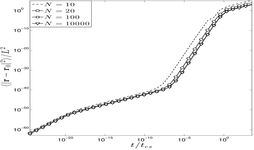
The principal results of this paper are as follows. For a general Gaussian model of Eulerian turbulence we carefully derive the diffusion approximation for pair dispersion assumed in the argument of Thomson-Devenish Thomson and Devenish (2005), under the assumption of short memory times for particle locations. We furthermore obtain a closed formula, eq.(84), for the 2-particle eddy-diffusivity in a general Gaussian model. For the specific models with covariance (3) we obtained more explicit results, which, under the conditions α<1𝛼1\alpha<1 and either β<1𝛽1\beta<1 or frozen turbulence with D3=0,subscript𝐷30D_{3}=0, verify the Thomson-Devenish argument about sweeping decorrelation effects. In particular, we obtain under these conditions a 2-particle eddy-diffusivity tensor of the form Kij(𝐫,t)=Sij(𝐫)τ(r,t),subscript𝐾𝑖𝑗𝐫𝑡subscript𝑆𝑖𝑗𝐫𝜏𝑟𝑡K_{ij}({\bf r},t)=S_{ij}({\bf r})\tau(r,t), where Sij(𝐫)subscript𝑆𝑖𝑗𝐫S_{ij}({\bf r}) is the structure-function tensor and τ(r,t)𝜏𝑟𝑡\tau(r,t) is an effective correlation time of velocity increments. Crucially, τ(r,t)𝜏𝑟𝑡\tau(r,t) is the minimum of the intrinsic turnover time τeddy(r)subscript𝜏𝑒𝑑𝑑𝑦𝑟\tau_{eddy}(r) at separation r𝑟r, the overall evolution time t,𝑡t, and the sweeping time r/v0.𝑟subscript𝑣0r/v_{0}. Although this result confirms the sweeping decorrelation effect, we argue that the pair-dispersion law for zero mean-velocity ensembles at high Reynolds numbers is different from the t9/2superscript𝑡92t^{9/2} suggested by Thomson & Devenish Thomson and Devenish (2005). Instead, we argue that there are distinct ranges of power-laws t2,superscript𝑡2t^{2}, t1,superscript𝑡1t^{1}, t6superscript𝑡6t^{6} and then t1superscript𝑡1t^{1} again at successively longer times, exactly as Thomson & Devenish argued for ensembles with large mean velocities. We carry out careful numerical Monte Carlo simulations with our diffusion model which verify these behaviors in the model at very high Reynolds numbers. We also present Monte Carlo results for our diffusion model at the moderate Reynolds numbers employed in current KS work, and reproduce then both the “t3superscript𝑡3t^{3}-law” and “t9/2superscript𝑡92t^{9/2}-law” that have been reported in KS at comparable Reynolds numbers. We thus argue that the current KS results in the literature are not yet probing asymptotic regimes and the true scaling in KS at very high Reynolds numbers will be the same as in our diffusion model.

The detailed analytical derivation of diffusion models is presented in section II of the paper, and predictions for their dispersion laws discussed in section III. Our numerical methods are described and validated in section IV , and then used to obtain results for mean-square particle separations and other statistics. A concluding section V briefly discusses the results.

II Derivation of the Diffusion Model

In this section we present the derivations of our main analytical results. A reader who is only interested in physical conclusions and not the detailed justifications may skip to our final formula (84) for the pair-diffusivity and the following discussion.

II.1 Gaussian Integration-by-Parts Identity

We show first that the transition probability of particle pairs in Gaussian velocity ensembles obeys an exact evolution equation, as a consequence of the well-known integration-by-parts identity or Donsker-Furutsu-Novikov relation (see Frisch (1995), section 4.1). Let 𝐮(𝐱,t)𝐮𝐱𝑡{\bf u}({\bf x},t) be the random turbulent velocity field and let the fluid particle position that satisfies

ddt𝐱(t)=𝐮(𝐱,t),𝐱(t0)=𝐚formulae-sequence𝑑𝑑𝑡𝐱𝑡𝐮𝐱𝑡𝐱subscript𝑡0𝐚{{d}\over{dt}}{\bf x}(t)={\bf u}({\bf x},t),\,\,\,\,{\bf x}(t_{0})={\bf a} (6)

be denoted as 𝐱𝐮(𝐚,t0|t)subscript𝐱𝐮𝐚conditionalsubscript𝑡0𝑡{\bf x}_{\bf u}({\bf a},t_{0}|t), or 𝐱(𝐚,t)𝐱𝐚𝑡{\bf x}({\bf a},t) for short. Define the “fine-grained PDF” of 2-particle positions as

P2,𝐮(𝐱2,𝐱1,t|𝐚2,𝐚1,t0)=n=12δd(𝐱n𝐱𝐮(𝐚n,t0|t)).subscript𝑃2𝐮subscript𝐱2subscript𝐱1conditional𝑡subscript𝐚2subscript𝐚1subscript𝑡0superscriptsubscriptproduct𝑛12superscript𝛿𝑑subscript𝐱𝑛subscript𝐱𝐮subscript𝐚𝑛conditionalsubscript𝑡0𝑡P_{2,{\bf u}}({\bf x}_{2},{\bf x}_{1},t|{\bf a}_{2},{\bf a}_{1},t_{0})=\prod_{n=1}^{2}\delta^{d}({\bf x}_{n}-{\bf x}_{\bf u}({\bf a}_{n},t_{0}|t)). (7)

Then the PDF of 2-particle positions is given by

P2(𝐱2,𝐱1,t|𝐚2,𝐚1,t0)=P2,𝐮(𝐱2,𝐱1,t|𝐚2,𝐚1,t0),subscript𝑃2subscript𝐱2subscript𝐱1conditional𝑡subscript𝐚2subscript𝐚1subscript𝑡0delimited-⟨⟩subscript𝑃2𝐮subscript𝐱2subscript𝐱1conditional𝑡subscript𝐚2subscript𝐚1subscript𝑡0P_{2}({\bf x}_{2},{\bf x}_{1},t|{\bf a}_{2},{\bf a}_{1},t_{0})=\langle P_{2,{\bf u}}({\bf x}_{2},{\bf x}_{1},t|{\bf a}_{2},{\bf a}_{1},t_{0})\rangle, (8)

where the average is over the random velocity field 𝐮.𝐮{\bf u}.

Taking the time-derivative of (7) and using (6) it is a calculus exercise to show that

tP2,𝐮(t)=n=12𝐱n[(𝐮¯(𝐱n,t)+𝐮(𝐱n,t))P2,𝐮(t)],subscript𝑡subscript𝑃2𝐮𝑡superscriptsubscript𝑛12bold-⋅subscriptsubscript𝐱𝑛delimited-[]¯𝐮subscript𝐱𝑛𝑡superscript𝐮subscript𝐱𝑛𝑡subscript𝑃2𝐮𝑡\partial_{t}P_{2,{\bf u}}(t)=-\sum_{n=1}^{2}\hbox{\boldmath$\nabla$}_{{\bf x}_{n}}\hbox{\boldmath$\cdot$}\left[(\overline{{\bf u}}({\bf x}_{n},t)+{\bf u}^{\prime}({\bf x}_{n},t))P_{2,{\bf u}}(t)\right], (9)

where the velocity has been decomposed into its mean and fluctuating part 𝐮(𝐱,t)=𝐮¯(𝐱,t)+𝐮(𝐱,t).𝐮𝐱𝑡¯𝐮𝐱𝑡superscript𝐮𝐱𝑡{\bf u}({\bf x},t)=\overline{{\bf u}}({\bf x},t)+{\bf u}^{\prime}({\bf x},t). The average of the second term on the righthand side can be obtained using Gaussian integration-by-parts Frisch (1995)

ui(𝐱,t))P2,𝐮(t)\displaystyle\langle u^{\prime}_{i}({\bf x},t))P_{2,{\bf u}}(t)\rangle =\displaystyle= ddy𝑑sCik(𝐱,t;𝐲,s)superscript𝑑𝑑𝑦differential-d𝑠subscript𝐶𝑖𝑘𝐱𝑡𝐲𝑠\displaystyle\int d^{d}y\int ds\,\,C_{ik}({\bf x},t;{\bf y},s) (11)
×δδuk(𝐲,s)P2,𝐮(t),absentdelimited-⟨⟩𝛿𝛿subscript𝑢𝑘𝐲𝑠subscript𝑃2𝐮𝑡\displaystyle\,\,\,\,\,\,\times\left\langle\frac{\delta}{\delta u_{k}({\bf y},s)}P_{2,{\bf u}}(t)\right\rangle,

where Cij(𝐱,t;𝐲,s)=ui(𝐱,t)uj(𝐲,s).subscript𝐶𝑖𝑗𝐱𝑡𝐲𝑠delimited-⟨⟩superscriptsubscript𝑢𝑖𝐱𝑡superscriptsubscript𝑢𝑗𝐲𝑠C_{ij}({\bf x},t;{\bf y},s)=\langle u_{i}^{\prime}({\bf x},t)u_{j}^{\prime}({\bf y},s)\rangle. To represent the functional derivative we introduce the Lagrangian response function

Gij(𝐚,t;𝐲,s)δxi(𝐚,t)δuj(𝐲,s),subscript𝐺𝑖𝑗𝐚𝑡𝐲𝑠𝛿subscript𝑥𝑖𝐚𝑡𝛿subscript𝑢𝑗𝐲𝑠G_{ij}({\bf a},t;{\bf y},s)\equiv\frac{\delta x_{i}({\bf a},t)}{\delta u_{j}({\bf y},s)}, (12)

so that

δδuk(𝐲,s)P2,𝐮(t)=m=12xmjP2,𝐮(t)Gjk(𝐚m,t;𝐲,s).𝛿𝛿subscript𝑢𝑘𝐲𝑠subscript𝑃2𝐮𝑡superscriptsubscript𝑚12subscriptsubscriptsuperscript𝑥𝑗𝑚subscript𝑃2𝐮𝑡subscript𝐺𝑗𝑘subscript𝐚𝑚𝑡𝐲𝑠\frac{\delta}{\delta u_{k}({\bf y},s)}P_{2,{\bf u}}(t)=\sum_{m=1}^{2}-\partial_{x^{j}_{m}}P_{2,{\bf u}}(t)\cdot G_{jk}({\bf a}_{m},t;{\bf y},s). (13)

The result of averaging (9) is the drift-diffusion equation

tP2(t)=n=12𝐱n[𝐮¯(𝐱n,t)P2(t)]subscript𝑡subscript𝑃2𝑡superscriptsubscript𝑛12bold-⋅subscriptbold-∇subscript𝐱𝑛delimited-[]superscript¯𝐮subscript𝐱𝑛𝑡subscript𝑃2𝑡\displaystyle\partial_{t}P_{2}(t)=-\sum_{n=1}^{2}\hbox{\boldmath$\nabla$}_{{\bf x}_{n}}\hbox{\boldmath$\cdot$}\left[\overline{{\bf u}}^{*}({\bf x}_{n},t)P_{2}(t)\right] (14)
+n,m=12xnixmj[Dij(𝐱n,𝐱m,t,t0)P2(t)].superscriptsubscript𝑛𝑚12subscriptsubscriptsuperscript𝑥𝑖𝑛subscriptsubscriptsuperscript𝑥𝑗𝑚delimited-[]subscript𝐷𝑖𝑗subscript𝐱𝑛subscript𝐱𝑚𝑡subscript𝑡0subscript𝑃2𝑡\displaystyle+\sum_{n,m=1}^{2}\partial_{x^{i}_{n}}\partial_{x^{j}_{m}}\left[D_{ij}({\bf x}_{n},{\bf x}_{m},t,t_{0})P_{2}(t)\right]. (15)

with

𝐮¯(𝐱,t)=𝐮¯(𝐱,t)+xjDij(𝐱,𝐱,t,t0)|𝐱=𝐱superscript¯𝐮𝐱𝑡¯𝐮𝐱𝑡evaluated-atsubscriptsuperscript𝑥𝑗subscript𝐷𝑖𝑗𝐱superscript𝐱𝑡subscript𝑡0superscript𝐱𝐱\overline{{\bf u}}^{*}({\bf x},t)=\overline{{\bf u}}({\bf x},t)+\left.\partial_{x^{j}}D_{ij}({\bf x},{\bf x}^{\prime},t,t_{0})\right|_{{\bf x}^{\prime}={\bf x}} (16)

the mean velocity plus a fluctuation-induced drift, and with the diffusivity tensor

Dij(𝐱n,𝐱m,t,t0)t0t𝑑sddyCik(𝐱n,t;𝐲,s)subscript𝐷𝑖𝑗subscript𝐱𝑛subscript𝐱𝑚𝑡subscript𝑡0superscriptsubscriptsubscript𝑡0𝑡differential-d𝑠superscript𝑑𝑑𝑦subscript𝐶𝑖𝑘subscript𝐱𝑛𝑡𝐲𝑠\displaystyle D_{ij}({\bf x}_{n},{\bf x}_{m},t,t_{0})\equiv\int_{t_{0}}^{t}ds\int d^{d}y\,\,C_{ik}({\bf x}_{n},t;{\bf y},s) (17)
×Gjk(𝐚m,t;𝐲,s)|𝐱2,𝐱1,t;𝐚2,𝐚1,t0absentinner-productsubscript𝐺𝑗𝑘subscript𝐚𝑚𝑡𝐲𝑠subscript𝐱2subscript𝐱1𝑡subscript𝐚2subscript𝐚1subscript𝑡0\displaystyle\,\,\,\,\,\,\,\,\,\,\,\,\,\,\,\,\,\,\,\,\,\,\,\,\times\langle G_{jk}({\bf a}_{m},t;{\bf y},s)|{\bf x}_{2},{\bf x}_{1},t;{\bf a}_{2},{\bf a}_{1},t_{0}\rangle (18)

where

Gjk(𝐚m,t;𝐲,s)|𝐱2,𝐱1,t;𝐚2,𝐚1,t0inner-productsubscript𝐺𝑗𝑘subscript𝐚𝑚𝑡𝐲𝑠subscript𝐱2subscript𝐱1𝑡subscript𝐚2subscript𝐚1subscript𝑡0\displaystyle\langle G_{jk}({\bf a}_{m},t;{\bf y},s)|{\bf x}_{2},{\bf x}_{1},t;{\bf a}_{2},{\bf a}_{1},t_{0}\rangle (19)
=Gjk(𝐚m,t;𝐲,s)P2,𝐮(t)P2(t)absentdelimited-⟨⟩subscript𝐺𝑗𝑘subscript𝐚𝑚𝑡𝐲𝑠subscript𝑃2𝐮𝑡subscript𝑃2𝑡\displaystyle\,\,\,\,\,\,\,\,\,\,\,\,\,\,\,\,\,\,\,\,\,\,\,\,\,\,\,\,\,\,\,\,\,\,\,\,\,\,\,\,=\frac{\langle G_{jk}({\bf a}_{m},t;{\bf y},s)P_{2,{\bf u}}(t)\rangle}{P_{2}(t)} (20)

is the conditional average of the response function given that the two particles start in locations 𝐚2,𝐚1subscript𝐚2subscript𝐚1{\bf a}_{2},{\bf a}_{1} at time t0subscript𝑡0t_{0} and end up at locations 𝐱2,𝐱1subscript𝐱2subscript𝐱1{\bf x}_{2},{\bf x}_{1} at time t.𝑡t.

We now develop a more useful expression for the response function (12). It is straightforward to show by functional differentiation of the equation of motion (6) that

tGij=uixk(𝐱(𝐚,t0|t),t)Gkj+δijδd(𝐲𝐱(𝐚,t0|t))δ(ts).subscript𝑡subscript𝐺𝑖𝑗subscript𝑢𝑖subscript𝑥𝑘𝐱𝐚conditionalsubscript𝑡0𝑡𝑡subscript𝐺𝑘𝑗subscript𝛿𝑖𝑗superscript𝛿𝑑𝐲𝐱𝐚conditionalsubscript𝑡0𝑡𝛿𝑡𝑠\partial_{t}G_{ij}=\frac{\partial u_{i}}{\partial x_{k}}({\bf x}({\bf a},t_{0}|t),t)G_{kj}+\delta_{ij}\delta^{d}({\bf y}-{\bf x}({\bf a},t_{0}|t))\delta(t-s). (21)

This equation may be solved as

Gij(𝐚,t;𝐲,s)={gij(𝐲,s|t)δd(𝐲𝐱(𝐚,t0|s))t>s>t00o.w.subscript𝐺𝑖𝑗𝐚𝑡𝐲𝑠casessubscript𝑔𝑖𝑗𝐲conditional𝑠𝑡superscript𝛿𝑑𝐲𝐱𝐚conditionalsubscript𝑡0𝑠𝑡𝑠subscript𝑡00formulae-sequenceowG_{ij}({\bf a},t;{\bf y},s)=\left\{\begin{array}[]{ll}g_{ij}({\bf y},s|t)\delta^{d}({\bf y}-{\bf x}({\bf a},t_{0}|s))&t>s>t_{0}\cr 0&{\rm o.w.}\cr\end{array}\right. (22)

with 𝐠(𝐲,s|t)=Texp(st𝑑r𝐮𝐱(𝐱(𝐚,t0|r),r))𝐠𝐲conditional𝑠𝑡Texpsuperscriptsubscript𝑠𝑡differential-d𝑟𝐮𝐱𝐱𝐚conditionalsubscript𝑡0𝑟𝑟{\bf g}({\bf y},s|t)={\rm Texp}\left(\int_{s}^{t}dr\,\frac{\partial{\bf u}}{\partial{\bf x}}({\bf x}({\bf a},t_{0}|r),r)\right) the time-ordered exponential matrix for the trajectory which satisfies 𝐱(𝐚,t0|s)=𝐲.𝐱𝐚conditionalsubscript𝑡0𝑠𝐲{\bf x}({\bf a},t_{0}|s)={\bf y}. This notation is made natural by an alternative derivation of (22) based on the flow composition identity

𝐱(𝐚,t0|t)=𝐱(𝐱(𝐚,t0|s),s|t).𝐱𝐚conditionalsubscript𝑡0𝑡𝐱𝐱𝐚conditionalsubscript𝑡0𝑠conditional𝑠𝑡{\bf x}({\bf a},t_{0}|t)={\bf x}({\bf x}({\bf a},t_{0}|s),s|t). (23)

Taking the functional derivative δ/δuj(𝐲,s)𝛿𝛿subscript𝑢𝑗𝐲𝑠\delta/\delta u_{j}({\bf y},s) of (23) and using the chain rule gives

δxi(𝐚,t)δuj(𝐲,s)=xiyk(𝐲,s|t)|𝐲=𝐱(𝐚,s)δxk(𝐚,s)δuj(𝐲,s).𝛿subscript𝑥𝑖𝐚𝑡𝛿subscript𝑢𝑗𝐲𝑠evaluated-atsubscript𝑥𝑖subscript𝑦𝑘𝐲conditional𝑠𝑡𝐲𝐱𝐚𝑠𝛿subscript𝑥𝑘𝐚𝑠𝛿subscript𝑢𝑗𝐲𝑠\frac{\delta x_{i}({\bf a},t)}{\delta u_{j}({\bf y},s)}=\left.\frac{\partial x_{i}}{\partial y_{k}}({\bf y},s|t)\right|_{{\bf y}={\bf x}({\bf a},s)}\frac{\delta x_{k}({\bf a},s)}{\delta u_{j}({\bf y},s)}. (24)

On the other hand, it is readily seen that the functional derivative of the integral form of the particle equation of motion (6), gives

δxk(𝐚,s)δuj(𝐲,s)=δjkδd(𝐲𝐱(𝐚,t0|s))θ(st0).𝛿subscript𝑥𝑘𝐚𝑠𝛿subscript𝑢𝑗𝐲𝑠subscript𝛿𝑗𝑘superscript𝛿𝑑𝐲𝐱𝐚conditionalsubscript𝑡0𝑠𝜃𝑠subscript𝑡0\frac{\delta x_{k}({\bf a},s)}{\delta u_{j}({\bf y},s)}=\delta_{jk}\delta^{d}({\bf y}-{\bf x}({\bf a},t_{0}|s))\theta(s-t_{0}). (25)

Thus, eq.(22) is rederived with gij(𝐲,s|t)=xiyj(𝐲,s|t).subscript𝑔𝑖𝑗𝐲conditional𝑠𝑡subscript𝑥𝑖subscript𝑦𝑗𝐲conditional𝑠𝑡g_{ij}({\bf y},s|t)=\frac{\partial x_{i}}{\partial y_{j}}({\bf y},s|t). If (22) is substituted into the formula (18) it yields

Dij(𝐱n,𝐱m,t,t0)t0t𝑑sddymCik(𝐱n,t;𝐲m,s)subscript𝐷𝑖𝑗subscript𝐱𝑛subscript𝐱𝑚𝑡subscript𝑡0superscriptsubscriptsubscript𝑡0𝑡differential-d𝑠superscript𝑑𝑑subscript𝑦𝑚subscript𝐶𝑖𝑘subscript𝐱𝑛𝑡subscript𝐲𝑚𝑠\displaystyle D_{ij}({\bf x}_{n},{\bf x}_{m},t,t_{0})\equiv\int_{t_{0}}^{t}ds\int d^{d}y_{m}\,\,C_{ik}({\bf x}_{n},t;{\bf y}_{m},s) (26)
×gjk(𝐲m,s|t)|𝐱2,𝐱1,t;𝐲m,s;𝐚2,𝐚1,t0absentdelimited-⟨⟩conditionalsubscript𝑔𝑗𝑘subscript𝐲𝑚conditional𝑠𝑡subscript𝐱2subscript𝐱1𝑡subscript𝐲𝑚𝑠subscript𝐚2subscript𝐚1subscript𝑡0\displaystyle\,\,\,\,\,\,\,\,\,\,\,\,\,\,\,\,\,\,\,\,\,\,\,\,\times\langle g_{jk}({\bf y}_{m},s|t)|{\bf x}_{2},{\bf x}_{1},t;{\bf y}_{m},s;{\bf a}_{2},{\bf a}_{1},t_{0}\rangle (27)
×P(𝐲m,s|𝐱2,𝐱1,t;𝐚2,𝐚1,t0)absent𝑃subscript𝐲𝑚conditional𝑠subscript𝐱2subscript𝐱1𝑡subscript𝐚2subscript𝐚1subscript𝑡0\displaystyle\,\,\,\,\,\,\,\,\,\,\,\,\,\,\,\,\,\,\,\,\,\,\,\,\times P({\bf y}_{m},s|{\bf x}_{2},{\bf x}_{1},t;{\bf a}_{2},{\bf a}_{1},t_{0}) (28)

where P(𝐲m,s|𝐱2,𝐱1,t;𝐚2,𝐚1,t0)𝑃subscript𝐲𝑚conditional𝑠subscript𝐱2subscript𝐱1𝑡subscript𝐚2subscript𝐚1subscript𝑡0P({\bf y}_{m},s|{\bf x}_{2},{\bf x}_{1},t;{\bf a}_{2},{\bf a}_{1},t_{0}) is the conditional probability density of the position of particle m𝑚m at time s𝑠s given the positions of both particles at times t𝑡t and t0.subscript𝑡0t_{0}. This formula for the diffusivity when substituted into (15),(16) gives the final form of our exact evolution equation for the 2-particle transition probability.

II.2 Markovian Approximation

Despite appearances, the evolution in the exact equation (15) is non-Markovian in general. It is clear from formula (28) that the 2-particle diffusion matrix is a function not only of the particle positions 𝐱1,𝐱2subscript𝐱1subscript𝐱2{\bf x}_{1},{\bf x}_{2} at time t,𝑡t, but also of the positions 𝐚1,𝐚2subscript𝐚1subscript𝐚2{\bf a}_{1},{\bf a}_{2} at time t0.subscript𝑡0t_{0}. This dependence was suppressed in our notations, but the evolution, in principle, retains a long-time memory of the initial conditions. Only in special cases can the evolution be shown to be Markovian. The famous example is the Gaussian velocity field that is delta-correlated in time, the so-called Kraichnan model Kraichnan (1968); Falkovich et al. (2001), for which

Cik(𝐱,t;𝐲,s)=Cik(𝐱,𝐲;t)δ(ts).subscript𝐶𝑖𝑘𝐱𝑡𝐲𝑠subscript𝐶𝑖𝑘𝐱𝐲𝑡𝛿𝑡𝑠C_{ik}({\bf x},t;{\bf y},s)=C_{ik}({\bf x},{\bf y};t)\delta(t-s). (29)

Substituting into (28) and using

gjk(𝐲m,t|t)=δjksubscript𝑔𝑗𝑘subscript𝐲𝑚conditional𝑡𝑡subscript𝛿𝑗𝑘g_{jk}({\bf y}_{m},t|t)=\delta_{jk} (30)

and

P(𝐲m,t|𝐱2,𝐱1,t;𝐚2,𝐚1,t0)=δd(𝐲m𝐱m)𝑃subscript𝐲𝑚conditional𝑡subscript𝐱2subscript𝐱1𝑡subscript𝐚2subscript𝐚1subscript𝑡0superscript𝛿𝑑subscript𝐲𝑚subscript𝐱𝑚P({\bf y}_{m},t|{\bf x}_{2},{\bf x}_{1},t;{\bf a}_{2},{\bf a}_{1},t_{0})=\delta^{d}({\bf y}_{m}-{\bf x}_{m}) (31)

gives (with the “1212\frac{1}{2} delta-function rule” for the upper limit of integration)

Dij(𝐱n,𝐱m,t,t0)=12Cij(𝐱n,𝐱m,t).subscript𝐷𝑖𝑗subscript𝐱𝑛subscript𝐱𝑚𝑡subscript𝑡012subscript𝐶𝑖𝑗subscript𝐱𝑛subscript𝐱𝑚𝑡D_{ij}({\bf x}_{n},{\bf x}_{m},t,t_{0})=\frac{1}{2}C_{ij}({\bf x}_{n},{\bf x}_{m},t).

Thus, in this case rigorously there is no dependence of the diffusion matrix 𝐃𝐃{\bf D} on 𝐚1,𝐚2subscript𝐚1subscript𝐚2{\bf a}_{1},{\bf a}_{2} and the well-known diffusion model is obtained Kraichnan (1968); Falkovich et al. (2001). Another example with Markovian particle evolution is the velocity field obtained as the superposition of Gaussian random wave trains with very high frequencies, so that the group velocity of the waves greatly exceeds the root-mean-square velocity Balk (2002). This example has direct relevance to KS simulations with “eddy-turnover frequency” ωn=λkn3E(kn)subscript𝜔𝑛𝜆superscriptsubscript𝑘𝑛3𝐸subscript𝑘𝑛\omega_{n}=\lambda\sqrt{k_{n}^{3}E(k_{n})} in the limit λ1much-greater-than𝜆1\lambda\gg 1 of large “unsteadiness” parameter.

The description as a diffusion should generally hold reasonably well if the correlation time of the Gaussian velocity field is short enough, since the integrand in (28) then becomes negligible at values of s<t𝑠𝑡s<t for which there is sizable dependence on 𝐚1,𝐚2subscript𝐚1subscript𝐚2{\bf a}_{1},{\bf a}_{2}. With this motivation, we make the Markovian approximation

Dij(𝐱n,𝐱m,t,t0)t0t𝑑sddymCik(𝐱n,t;𝐲m,s)subscript𝐷𝑖𝑗subscript𝐱𝑛subscript𝐱𝑚𝑡subscript𝑡0superscriptsubscriptsubscript𝑡0𝑡differential-d𝑠superscript𝑑𝑑subscript𝑦𝑚subscript𝐶𝑖𝑘subscript𝐱𝑛𝑡subscript𝐲𝑚𝑠\displaystyle D_{ij}({\bf x}_{n},{\bf x}_{m},t,t_{0})\equiv\int_{t_{0}}^{t}ds\int d^{d}y_{m}\,\,C_{ik}({\bf x}_{n},t;{\bf y}_{m},s) (32)
×gjk(𝐲m,s|t)|𝐱2,𝐱1,t;𝐲m,sP(𝐲m,s|𝐱2,𝐱1,t).absentdelimited-⟨⟩conditionalsubscript𝑔𝑗𝑘subscript𝐲𝑚conditional𝑠𝑡subscript𝐱2subscript𝐱1𝑡subscript𝐲𝑚𝑠𝑃subscript𝐲𝑚conditional𝑠subscript𝐱2subscript𝐱1𝑡\displaystyle\,\,\times\langle g_{jk}({\bf y}_{m},s|t)|{\bf x}_{2},{\bf x}_{1},t;{\bf y}_{m},s\rangle P({\bf y}_{m},s|{\bf x}_{2},{\bf x}_{1},t). (33)

The physical assumption is that for times ordered as t0s<tmuch-less-thansubscript𝑡0𝑠𝑡t_{0}\ll s<t the position of the particle at time s𝑠s is determined mainly by its position at time t𝑡t and is negligibly dependent on the position at the initial time t0subscript𝑡0t_{0}. The worst case for this approximation is clearly the “frozen velocity” model with infinite correlation time, when times st0greater-than-or-equivalent-to𝑠subscript𝑡0s\gtrsim t_{0} in the integral are not suppressed by decay of correlations. Such s𝑠s values give an undamped contribution also in general for times tt0𝑡subscript𝑡0t-t_{0} much smaller than the velocity correlation time. However, it is easy to check that the exact result (18) [or (28)] and the Markovianized result (33) both give

ddtDij(𝐱n,𝐱m,t,t0)=Cij(𝐱n,t;𝐱m,t)+O(tt0)𝑑𝑑𝑡subscript𝐷𝑖𝑗subscript𝐱𝑛subscript𝐱𝑚𝑡subscript𝑡0subscript𝐶𝑖𝑗subscript𝐱𝑛𝑡subscript𝐱𝑚𝑡𝑂𝑡subscript𝑡0\frac{d}{dt}D_{ij}({\bf x}_{n},{\bf x}_{m},t,t_{0})=C_{ij}({\bf x}_{n},t;{\bf x}_{m},t)+O(t-t_{0}) (34)

so that, for tt0𝑡subscript𝑡0t-t_{0} much smaller than the correlation time,

Dij(𝐱n,𝐱m,t,t0)=Cij(𝐱n,t0;𝐱m,t0)(tt0)+O((tt0)2).subscript𝐷𝑖𝑗subscript𝐱𝑛subscript𝐱𝑚𝑡subscript𝑡0subscript𝐶𝑖𝑗subscript𝐱𝑛subscript𝑡0subscript𝐱𝑚subscript𝑡0𝑡subscript𝑡0𝑂superscript𝑡subscript𝑡02D_{ij}({\bf x}_{n},{\bf x}_{m},t,t_{0})=C_{ij}({\bf x}_{n},t_{0};{\bf x}_{m},t_{0})(t-t_{0})+O((t-t_{0})^{2}). (35)

Thus the Markovian approximation becomes exact in this limit. We note in passing that the Kraichnan-Lundgren theory of 2-particle dispersion Kraichnan (1966); Lundgren (1981) when applied to the Gaussian velocity ensemble gives a result almost identical to the formula (33) (for more discussion, see Eyink (2012)).

The formula (33) from the Markovian approximation can be further simplified. It is intuitively clear that conditioning on the location of both particles is superfluous in an average of a random variable that involves only one of these particles. In fact, it can be easily established from the definitions (7),(8) that

P(𝐲,s|𝐱,𝐱,t)𝑃𝐲conditional𝑠superscript𝐱𝐱𝑡\displaystyle P({\bf y},s|{\bf x}^{\prime},{\bf x},t) =\displaystyle= ddyP(𝐲,𝐲,s|𝐱,𝐱,t)superscript𝑑𝑑superscript𝑦𝑃superscript𝐲𝐲conditional𝑠superscript𝐱𝐱𝑡\displaystyle\int d^{d}y^{\prime}\,P({\bf y}^{\prime},{\bf y},s|{\bf x}^{\prime},{\bf x},t) (36)
=\displaystyle= ddyδd(𝐲𝐱(𝐱,t|s))δd(𝐲𝐱(𝐱,t|s))superscript𝑑𝑑superscript𝑦delimited-⟨⟩superscript𝛿𝑑superscript𝐲𝐱superscript𝐱conditional𝑡𝑠superscript𝛿𝑑𝐲𝐱𝐱conditional𝑡𝑠\displaystyle\int d^{d}y^{\prime}\,\langle\delta^{d}({\bf y}^{\prime}-{\bf x}({\bf x}^{\prime},t|s))\delta^{d}({\bf y}-{\bf x}({\bf x},t|s))\rangle (37)
=\displaystyle= δd(𝐲𝐱(𝐱,t|s))=P(𝐲,s|𝐱,t).delimited-⟨⟩superscript𝛿𝑑𝐲𝐱𝐱conditional𝑡𝑠𝑃𝐲conditional𝑠𝐱𝑡\displaystyle\langle\delta^{d}({\bf y}-{\bf x}({\bf x},t|s))\rangle=P({\bf y},s|{\bf x},t). (38)

A similar argument gives

gjk(𝐲,s|t)|𝐱,𝐱,t;𝐲,s=gjk(𝐲,s|t)|𝐱,t;𝐲,s.delimited-⟨⟩conditionalsubscript𝑔𝑗𝑘𝐲conditional𝑠𝑡superscript𝐱𝐱𝑡𝐲𝑠delimited-⟨⟩conditionalsubscript𝑔𝑗𝑘𝐲conditional𝑠𝑡𝐱𝑡𝐲𝑠\langle g_{jk}({\bf y},s|t)|{\bf x}^{\prime},{\bf x},t;{\bf y},s\rangle=\langle g_{jk}({\bf y},s|t)|{\bf x},t;{\bf y},s\rangle. (39)

More generally, we may define the PDF

P(𝐠,t;𝐲,𝐲,s|𝐱,𝐱,t)=𝑃𝐠𝑡superscript𝐲𝐲conditional𝑠superscript𝐱𝐱𝑡absent\displaystyle P({\bf g},t;{\bf y}^{\prime},{\bf y},s|{\bf x}^{\prime},{\bf x},t)= (40)
δd×d(𝐠𝐠(𝐲,s|t))δd(𝐲𝐱(𝐱,t|s))δd(𝐲𝐱(𝐱,t|s))delimited-⟨⟩superscript𝛿𝑑𝑑𝐠𝐠𝐲conditional𝑠𝑡superscript𝛿𝑑superscript𝐲𝐱superscript𝐱conditional𝑡𝑠superscript𝛿𝑑𝐲𝐱𝐱conditional𝑡𝑠\displaystyle\langle\delta^{d\times d}({\bf g}-{\bf g}({\bf y},s|t))\delta^{d}({\bf y}^{\prime}-{\bf x}({\bf x}^{\prime},t|s))\delta^{d}({\bf y}-{\bf x}({\bf x},t|s))\rangle (41)

and mimic the previous argument to show that

P(𝐠,t;𝐲,s|𝐱,𝐱,t)=P(𝐠,t;𝐲,s|𝐱,t).𝑃𝐠𝑡𝐲conditional𝑠superscript𝐱𝐱𝑡𝑃𝐠𝑡𝐲conditional𝑠𝐱𝑡P({\bf g},t;{\bf y},s|{\bf x}^{\prime},{\bf x},t)=P({\bf g},t;{\bf y},s|{\bf x},t). (43)

Then

P(𝐠,t|𝐲,s;𝐱,𝐱,t)𝑃𝐠conditional𝑡𝐲𝑠superscript𝐱𝐱𝑡\displaystyle P({\bf g},t|{\bf y},s;{\bf x}^{\prime},{\bf x},t) =\displaystyle= P(𝐠,t;𝐲,s|𝐱,𝐱,t)P(𝐲,s|𝐱,𝐱,t)𝑃𝐠𝑡𝐲conditional𝑠superscript𝐱𝐱𝑡𝑃𝐲conditional𝑠superscript𝐱𝐱𝑡\displaystyle\frac{P({\bf g},t;{\bf y},s|{\bf x}^{\prime},{\bf x},t)}{P({\bf y},s|{\bf x}^{\prime},{\bf x},t)} (44)
=\displaystyle= P(𝐠,t;𝐲,s|𝐱,t)P(𝐲,s|𝐱,t)𝑃𝐠𝑡𝐲conditional𝑠𝐱𝑡𝑃𝐲conditional𝑠𝐱𝑡\displaystyle\frac{P({\bf g},t;{\bf y},s|{\bf x},t)}{P({\bf y},s|{\bf x},t)} (45)
=\displaystyle= P(𝐠,t|𝐲,s;𝐱,t).𝑃𝐠conditional𝑡𝐲𝑠𝐱𝑡\displaystyle P({\bf g},t|{\bf y},s;{\bf x},t). (46)

It follows from these facts that

Dij(𝐱n,𝐱m,t,t0)t0t𝑑sddymCik(𝐱n,t;𝐲m,s)subscript𝐷𝑖𝑗subscript𝐱𝑛subscript𝐱𝑚𝑡subscript𝑡0superscriptsubscriptsubscript𝑡0𝑡differential-d𝑠superscript𝑑𝑑subscript𝑦𝑚subscript𝐶𝑖𝑘subscript𝐱𝑛𝑡subscript𝐲𝑚𝑠\displaystyle D_{ij}({\bf x}_{n},{\bf x}_{m},t,t_{0})\equiv\int_{t_{0}}^{t}ds\int d^{d}y_{m}\,\,C_{ik}({\bf x}_{n},t;{\bf y}_{m},s) (47)
×gjk(𝐲m,s|t)|𝐱m,t;𝐲m,sP(𝐲m,s|𝐱m,t),absentdelimited-⟨⟩conditionalsubscript𝑔𝑗𝑘subscript𝐲𝑚conditional𝑠𝑡subscript𝐱𝑚𝑡subscript𝐲𝑚𝑠𝑃subscript𝐲𝑚conditional𝑠subscript𝐱𝑚𝑡\displaystyle\,\,\,\,\times\langle g_{jk}({\bf y}_{m},s|t)|{\bf x}_{m},t;{\bf y}_{m},s\rangle P({\bf y}_{m},s|{\bf x}_{m},t), (48)

which is the final form of the Markovian approximation for the diffusion tensor.

We now consider the special case when the velocity field is statistically homogeneous in space. In that case, the drift velocity in (16) is independent of 𝐱𝐱{\bf x} and simplifies to 𝐮¯(t)=𝐮¯(t),superscript¯𝐮𝑡¯𝐮𝑡\overline{{\bf u}}^{*}(t)=\overline{{\bf u}}(t), due to homogeneity and incompressibility 222This is the first point where we have invoked incompressibility.. Furthermore, a simplified equation can be derived for the transition probability of the 2-particle separation vector 𝐫=𝐱2𝐱1,𝐫subscript𝐱2subscript𝐱1{\bf r}={\bf x}_{2}-{\bf x}_{1}, defined by

P2(𝐫,t|𝐫0,t0)subscript𝑃2𝐫conditional𝑡subscript𝐫0subscript𝑡0\displaystyle P_{2}({\bf r},t|{\bf r}_{0},t_{0}) =\displaystyle= ddaP2(𝐱+𝐫,𝐱,t|𝐚+𝐫0,𝐚,t0)superscript𝑑𝑑𝑎subscript𝑃2𝐱𝐫𝐱conditional𝑡𝐚subscript𝐫0𝐚subscript𝑡0\displaystyle\int d^{d}a\,\,P_{2}({\bf x}+{\bf r},{\bf x},t|{\bf a}+{\bf r}_{0},{\bf a},t_{0}) (49)
=\displaystyle= ddaP2(𝐱,𝐱𝐫,t|𝐚+𝐫0,𝐚,t0),superscript𝑑𝑑𝑎subscript𝑃2𝐱𝐱𝐫conditional𝑡𝐚subscript𝐫0𝐚subscript𝑡0\displaystyle\int d^{d}a\,\,P_{2}({\bf x},{\bf x}-{\bf r},t|{\bf a}+{\bf r}_{0},{\bf a},t_{0}), (50)
(51)

which is also independent of 𝐱.𝐱{\bf x}. Since the diffusion tensor Dij(𝐱n,𝐱m,t)subscript𝐷𝑖𝑗subscript𝐱𝑛subscript𝐱𝑚𝑡D_{ij}({\bf x}_{n},{\bf x}_{m},t) depends only on the difference 𝐱n𝐱msubscript𝐱𝑛subscript𝐱𝑚{\bf x}_{n}-{\bf x}_{m} in the homogeneous case, the equation (15) with the substitutions 𝐫=𝐱2𝐱1𝐫subscript𝐱2subscript𝐱1{\bf r}={\bf x}_{2}-{\bf x}_{1} and

𝐱2𝐫,𝐱1𝐫,formulae-sequencesubscriptsubscript𝐱2subscript𝐫subscriptsubscript𝐱1subscript𝐫\hbox{\boldmath$\nabla$}_{{\bf x}_{2}}\longrightarrow\hbox{\boldmath$\nabla$}_{\bf r},\,\,\,\,\hbox{\boldmath$\nabla$}_{{\bf x}_{1}}\longrightarrow-\hbox{\boldmath$\nabla$}_{\bf r}, (52)

yields the diffusion equation

tP2(𝐫,t|𝐫0,t0)=rirj[Kij(𝐫,t,t0)P2(𝐫,t|𝐫0,t0)],subscript𝑡subscript𝑃2𝐫conditional𝑡subscript𝐫0subscript𝑡0subscriptsuperscript𝑟𝑖subscriptsuperscript𝑟𝑗delimited-[]subscript𝐾𝑖𝑗𝐫𝑡subscript𝑡0subscript𝑃2𝐫conditional𝑡subscript𝐫0subscript𝑡0\partial_{t}P_{2}({\bf r},t|{\bf r}_{0},t_{0})=\partial_{r^{i}}\partial_{r^{j}}\left[K_{ij}({\bf r},t,t_{0})P_{2}({\bf r},t|{\bf r}_{0},t_{0})\right], (53)

with the eddy-diffusivity tensor

Kij(𝐫,t,t0)subscript𝐾𝑖𝑗𝐫𝑡subscript𝑡0\displaystyle K_{ij}({\bf r},t,t_{0}) (54)
=2Dij(𝟎,𝟎,t,t0)Dij(𝐫,𝟎,t,t0)Dij(𝟎,𝐫,t,t0)absent2subscript𝐷𝑖𝑗00𝑡subscript𝑡0subscript𝐷𝑖𝑗𝐫0𝑡subscript𝑡0subscript𝐷𝑖𝑗0𝐫𝑡subscript𝑡0\displaystyle=2D_{ij}(\hbox{\boldmath$0$},\hbox{\boldmath$0$},t,t_{0})-D_{ij}({\bf r},\hbox{\boldmath$0$},t,t_{0})-D_{ij}(\hbox{\boldmath$0$},{\bf r},t,t_{0}) (55)
=t0t𝑑sddySik(𝐫;𝐲,t,s)absentsuperscriptsubscriptsubscript𝑡0𝑡differential-d𝑠superscript𝑑𝑑𝑦subscript𝑆𝑖𝑘𝐫𝐲𝑡𝑠\displaystyle=\int_{t_{0}}^{t}ds\int d^{d}y\,S_{ik}({\bf r};{\bf y},t,s) (56)
×gjk(𝐲,s|t)|𝟎,t;𝐲,sP(𝐲,s|𝟎,t)absentdelimited-⟨⟩conditionalsubscript𝑔𝑗𝑘𝐲conditional𝑠𝑡0𝑡𝐲𝑠𝑃𝐲conditional𝑠0𝑡\displaystyle\,\,\,\,\,\,\,\,\,\,\,\,\,\,\,\,\,\,\,\,\,\,\,\,\,\,\,\,\,\,\times\langle g_{jk}({\bf y},s|t)|\hbox{\boldmath$0$},t;{\bf y},s\rangle P({\bf y},s|\hbox{\boldmath$0$},t) (57)
(58)

and we define the 2nd-order structure function of velocity increments at two points 𝟎,𝐲0𝐲\hbox{\boldmath$0$},{\bf y} and two times t,s::𝑡𝑠absentt,s:

Sik(𝐫;𝐲,t,s)=[ui(𝐫,t)ui(𝟎,t)][uk(𝐲+𝐫,s)uk(𝐲,s)].subscript𝑆𝑖𝑘𝐫𝐲𝑡𝑠delimited-⟨⟩delimited-[]superscriptsubscript𝑢𝑖𝐫𝑡superscriptsubscript𝑢𝑖0𝑡delimited-[]superscriptsubscript𝑢𝑘𝐲𝐫𝑠superscriptsubscript𝑢𝑘𝐲𝑠S_{ik}({\bf r};{\bf y},t,s)=\langle[u_{i}^{\prime}({\bf r},t)-u_{i}^{\prime}(\hbox{\boldmath$0$},t)][u_{k}^{\prime}({\bf y}+{\bf r},s)-u_{k}^{\prime}({\bf y},s)]\rangle. (59)

If furthermore the velocity field is assumed to be statistically stationary in time, then we can take tt0t𝑡subscript𝑡0𝑡t-t_{0}\longrightarrow t and t00subscript𝑡00t_{0}\longrightarrow 0, to obtain

tP2(𝐫,t|𝐫0,0)=rirj[Kij(𝐫,t)P2(𝐫,t|𝐫0,0)],subscript𝑡subscript𝑃2𝐫conditional𝑡subscript𝐫00subscriptsuperscript𝑟𝑖subscriptsuperscript𝑟𝑗delimited-[]subscript𝐾𝑖𝑗𝐫𝑡subscript𝑃2𝐫conditional𝑡subscript𝐫00\partial_{t}P_{2}({\bf r},t|{\bf r}_{0},0)=\partial_{r^{i}}\partial_{r^{j}}\left[K_{ij}({\bf r},t)P_{2}({\bf r},t|{\bf r}_{0},0)\right], (60)

with

Kij(𝐫,t)=t0𝑑τddySik(𝐫;𝐲,0,τ)subscript𝐾𝑖𝑗𝐫𝑡superscriptsubscript𝑡0differential-d𝜏superscript𝑑𝑑𝑦subscript𝑆𝑖𝑘𝐫𝐲0𝜏\displaystyle K_{ij}({\bf r},t)=\int_{-t}^{0}d\tau\int d^{d}y\,S_{ik}({\bf r};{\bf y},0,\tau) (61)
×gjk(𝐲,τ|0)|𝟎,0;𝐲,τP(𝐲,τ|𝟎,0)absentdelimited-⟨⟩conditionalsubscript𝑔𝑗𝑘𝐲conditional𝜏000𝐲𝜏𝑃𝐲conditional𝜏00\displaystyle\,\,\,\,\,\,\,\,\,\,\,\times\langle g_{jk}({\bf y},\tau|0)|\hbox{\boldmath$0$},0;{\bf y},\tau\rangle P({\bf y},\tau|\hbox{\boldmath$0$},0) (62)

by the change of variables τ=st.𝜏𝑠𝑡\tau=s-t.

II.3 Structure Function and One-Particle Distribution Function

The integral over 𝐲𝐲{\bf y} in the above formula (62) converges at large y𝑦y because of decay in the two-point structure function and in the 1-particle transition probability. Physically, rapid decay is due to the facts that increments separated by great distances are uncorrelated and particles have low probability to be swept to large distances. Both of these effects can be easily quantified.

To evaluate the two-point structure function, we use a standard identity that expresses it in terms of the single-point 2nd-order structure function (Monin and Yaglom (1975), p.102):

Sik(𝐫;𝐲,0,τ)=12[Sik(𝐲+𝐫,0,τ)+Sik(𝐲𝐫,0,τ)\displaystyle S_{ik}({\bf r};{\bf y},0,\tau)=\frac{1}{2}\left[S_{ik}({\bf y}+{\bf r},0,\tau)+S_{ik}({\bf y}-{\bf r},0,\tau)\right. (63)
2Sik(𝐲,0,τ)].\displaystyle\,\,\,\,\,\,\,\,\,\,\,\,\,\,\,\,\,\,\,\,\,\,\,\,\,\,\,\,\,\,\,\,\,\,\,\,\,\,\,\,\,\,\,\,\,\,\,\,\,\,\,\,\,\,\,\,\,\,\,\,\,\,\,\,\,\,\,\,\left.-2S_{ik}({\bf y},0,\tau)\right]. (64)

We first consider the single-time case with τ=0.𝜏0\tau=0. For the spatial power-law covariance (5) with 0<α<20𝛼20<\alpha<2, the single-point structure function becomes

Sij(𝐫)=2[Cij(𝟎,τ)Cij(𝐫,τ)]|τ=0subscript𝑆𝑖𝑗𝐫evaluated-at2delimited-[]subscript𝐶𝑖𝑗0𝜏subscript𝐶𝑖𝑗𝐫𝜏𝜏0\displaystyle S_{ij}({\bf r})=\left.2\left[C_{ij}(\hbox{\boldmath$0$},\tau)-C_{ij}({\bf r},\tau)\right]\right|_{\tau=0} (65)
2D1rα[(d+α1)δijαr^ir^j]+O(r2/L2)similar-toabsent2subscript𝐷1superscript𝑟𝛼delimited-[]𝑑𝛼1subscript𝛿𝑖𝑗𝛼subscript^𝑟𝑖subscript^𝑟𝑗𝑂superscript𝑟2superscript𝐿2\displaystyle\,\,\,\,\sim 2D_{1}r^{\alpha}\left[(d+\alpha-1)\delta_{ij}-\alpha\hat{r}_{i}\hat{r}_{j}\right]+O(r^{2}/L^{2}) (66)

for rL.much-less-than𝑟𝐿r\ll L. The formula (64) implies in general that Sik(𝐫;𝐲,0,τ=0)Sik(𝐫)similar-tosubscript𝑆𝑖𝑘𝐫𝐲0𝜏0subscript𝑆𝑖𝑘𝐫S_{ik}({\bf r};{\bf y},0,\tau=0)\sim S_{ik}({\bf r}) for yr,much-less-than𝑦𝑟y\ll r, whereas in the particular case (66) it gives

Sik(𝐫;𝐲,0,τ=0)=O(r2/y2α)subscript𝑆𝑖𝑘𝐫𝐲0𝜏0𝑂superscript𝑟2superscript𝑦2𝛼S_{ik}({\bf r};{\bf y},0,\tau=0)=O(r^{2}/y^{2-\alpha}) (67)

for ryL.much-less-than𝑟𝑦much-less-than𝐿r\ll y\ll L. When yL,much-greater-than𝑦𝐿y\gg L, there is generally exponential or fast power-law decay, depending on the precise assumptions about the fall-off of the spectrum at low k.𝑘k. The 2-time structure function Sij(𝐫;0,τ)subscript𝑆𝑖𝑗𝐫0𝜏S_{ij}({\bf r};0,\tau) shows a similar behavior as the single-time structure function, except that there is a new length Lβ(τ)=(D3|τ|)1/βsubscript𝐿𝛽𝜏superscriptsubscript𝐷3𝜏1𝛽L_{\beta}(\tau)=(D_{3}|\tau|)^{1/\beta} with eddies smaller than this scale decorrelated by time |τ|.𝜏|\tau|. As seen from (3), the decorrelation is associated to an exponential decay of the cospectrum, with Lβ(t)subscript𝐿𝛽𝑡L_{\beta}(t) acting as an effective “dissipation scale.” Thus, Sij(𝐫;0,τ)subscript𝑆𝑖𝑗𝐫0𝜏S_{ij}({\bf r};0,\tau) scales r2proportional-toabsentsuperscript𝑟2\propto r^{2} for rLβ(τ),much-less-than𝑟subscript𝐿𝛽𝜏r\ll L_{\beta}(\tau), while formula (66) holds for Lβ(τ)rL.much-less-thansubscript𝐿𝛽𝜏𝑟much-less-than𝐿L_{\beta}(\tau)\ll r\ll L. Thus, the decay law (67) is found when τ0𝜏0\tau\neq 0 only for the range of values max{r,Lβ(τ)}yLmuch-less-than𝑟subscript𝐿𝛽𝜏𝑦much-less-than𝐿\max\{r,L_{\beta}(\tau)\}\ll y\ll L and is limited to times |τ|<Lβ/D3.𝜏superscript𝐿𝛽subscript𝐷3|\tau|<L^{\beta}/D_{3}. For ymax{r,Lβ(τ)}much-less-than𝑦𝑟subscript𝐿𝛽𝜏y\ll\max\{r,L_{\beta}(\tau)\} instead Sik(𝐫;𝐲,0,τ)subscript𝑆𝑖𝑘𝐫𝐲0𝜏S_{ik}({\bf r};{\bf y},0,\tau) is independent of 𝐲𝐲{\bf y} and for yLmuch-greater-than𝑦𝐿y\gg L the decay is again like that for τ=0.𝜏0\tau=0.

The 1-particle transition probability should be dominated by large-scale sweeping and thus have the form

P(𝐲,τ|𝟎,0)=1(2π)d/2v0d|τ|dexp(|𝐲𝐮¯τ|2/2v02τ2)𝑃𝐲conditional𝜏001superscript2𝜋𝑑2superscriptsubscript𝑣0𝑑superscript𝜏𝑑superscript𝐲¯𝐮𝜏22superscriptsubscript𝑣02superscript𝜏2P({\bf y},\tau|\hbox{\boldmath$0$},0)=\frac{1}{(2\pi)^{d/2}v_{0}^{d}|\tau|^{d}}\exp(-|{\bf y}-\overline{{\bf u}}\tau|^{2}/2v_{0}^{2}\tau^{2}) (68)

to a good approximation, with v0subscript𝑣0v_{0} the root mean square velocity. We hereafter consider mainly the case 𝐮¯=𝟎.¯𝐮0\overline{{\bf u}}=\hbox{\boldmath$0$}. For the Gaussian random field with mean zero and covariance (3), v0D2Lα.proportional-tosubscript𝑣0subscript𝐷2superscript𝐿𝛼v_{0}\propto D_{2}L^{\alpha}. In that case, it has been verified by a formal scaling analysis in Chaves et al. (2003), section 7, that the leading-order motion of particles for large L𝐿L is indeed ballistic with a constant, random velocity 𝐯=𝐲/τ𝐯𝐲𝜏{\bf v}={\bf y}/\tau chosen from a Gaussian ensemble with rms value v0.subscript𝑣0v_{0}. Subleading corrections were also obtained in Chaves et al. (2003) to account for the effects of the change of the velocity in space and time. Note that (68) decays rapidly for yv0|τ|.much-greater-than𝑦subscript𝑣0𝜏y\gg v_{0}|\tau|.

II.4 Stability Matrix

The most difficult term to evaluate in (62) is the conditional average of the stability matrix 𝐠(𝐲,τ|0).𝐠𝐲conditional𝜏0{\bf g}({\bf y},\tau|0). Existence of this matrix requires a short-distance cutoff η𝜂\eta on the “inertial-range” scaling behavior in the model covariance (3) and (5), which otherwise corresponds to velocity fields only Hölder continuous and non-differentiable in space. Even with the cutoff, the matrix 𝐠(𝐲,τ|0)𝐠𝐲conditional𝜏0{\bf g}({\bf y},\tau|0) will grow exponentially in |τ|𝜏|\tau| almost surely, with rate determined by the leading Lyapunov exponent λ(D1/η2α)1/2.proportional-to𝜆superscriptsubscript𝐷1superscript𝜂2𝛼12\lambda\propto(D_{1}/\eta^{2-\alpha})^{1/2}. It is thus far from clear a priori that the conditional average even remains finite in the limit η0.𝜂0\eta\rightarrow 0.

We begin by evaluating this term for the “frozen” velocity field with infinite correlation time (or D3=0subscript𝐷30D_{3}=0 in eq.(3)). A key observation here is that the Gaussian transition probability (68) implies that particles are swept from point 𝐲𝐲{\bf y} to 𝟎0 in time |τ|𝜏|\tau| along straight lines with a constant speed v=y/τ𝑣𝑦𝜏v=y/\tau generally of order v0.subscript𝑣0v_{0}. The velocity-gradient field 𝐮(𝐱,t)𝐮𝐱𝑡\hbox{\boldmath$\nabla$}{\bf u}({\bf x},t) has a spatial correlation of order η,𝜂\eta, so that the particle trajectories contributing in (62) will see a constant in space but rapidly changing velocity-gradient with a correlation time η/v0.similar-toabsent𝜂subscript𝑣0\sim\eta/v_{0}. Thus, one can expect that the Lagrangian velocity-gradient will be well approximated by the model of a Gaussian field that is delta-correlated in time, for which the statistics of the stability matrix has been much studied.

To make this argument more formally, consider the spatial covariance of the velocity-gradient in the frozen case Cij,mn(𝐫)=ui,m(𝐫)uj,n(𝟎),subscript𝐶𝑖𝑗𝑚𝑛𝐫delimited-⟨⟩superscriptsubscript𝑢𝑖𝑚𝐫superscriptsubscript𝑢𝑗𝑛0C_{ij,mn}({\bf r})=\langle u_{i,m}^{\prime}({\bf r})u_{j,n}^{\prime}(\hbox{\boldmath$0$})\rangle, where ui,m=ui/xm.superscriptsubscript𝑢𝑖𝑚superscriptsubscript𝑢𝑖subscript𝑥𝑚u_{i,m}^{\prime}=\partial u_{i}^{\prime}/\partial x_{m}. By twice differentiating (5) and then averaging over the direction of the unit vector 𝐫^,^𝐫\hat{{\bf r}}, it is calculated to be

C¯ij,mn(r)=D1rα2[(d+1)δijδmn\displaystyle\overline{C}_{ij,mn}(r)=D^{\prime}_{1}r^{\alpha-2}\left[(d+1)\delta_{ij}\delta_{mn}\right. (69)
(δimδjn+δinδjm)]\displaystyle\,\,\,\,\,\,\,\,\,\,\,\,\,\,\,\,\,\,\,\,\,\,\,\,\,\,\,\,\,\,\,\,\,\,\,\,\,\,\,\,\,\,\,\,\,\,\,\,\,\,\,\,\,\,\,\,\,\,\,\,\,\,\,\,\,\,\left.-(\delta_{im}\delta_{jn}+\delta_{in}\delta_{jm})\right] (70)

with D1=D1α(α2)d[α4d+2+2+dα2]>0subscriptsuperscript𝐷1subscript𝐷1𝛼𝛼2𝑑delimited-[]𝛼4𝑑22𝑑𝛼20D^{\prime}_{1}=\frac{D_{1}\alpha(\alpha-2)}{d}\left[\frac{\alpha-4}{d+2}+2+\frac{d}{\alpha-2}\right]>0 for d2𝑑2d\geq 2 and 0<α<2.0𝛼20<\alpha<2. This covariance holds for r>η,𝑟𝜂r>\eta, whereas the covariance for r<η𝑟𝜂r<\eta is essentially constant and can be taken to be given by (70) with r=η.𝑟𝜂r=\eta. A particle swept with velocity v𝑣v will see a random velocity-gradient with temporal correlation obtained by substituting r=vt𝑟𝑣𝑡r=vt in (70). Thus, the (Eulerian) velocity-gradients in a Lagrangian frame can be taken as Gaussian with covariance

ui,m(t)uj,n(0)=D1′′ηα1vδη(t)[(d+1)δijδmn\displaystyle\langle u_{i,m}^{\prime}(t)u_{j,n}^{\prime}(0)\rangle=D_{1}^{\prime\prime}\frac{\eta^{\alpha-1}}{v}\delta_{\eta}(t)\left[(d+1)\delta_{ij}\delta_{mn}\right. (71)
(δimδjn+δinδjm)]\displaystyle\,\,\,\,\,\,\,\,\,\,\,\,\,\,\,\,\,\,\,\,\,\,\,\,\,\,\,\,\,\,\,\,\,\,\,\,\,\,\,\,\,\,\,\,\,\,\,\,\,\,\,\,\,\,\,\,\,\,\,\,\,\,\,\,\,\,\left.-(\delta_{im}\delta_{jn}+\delta_{in}\delta_{jm})\right] (72)

with D1′′=2(2α1α)D1superscriptsubscript𝐷1′′22𝛼1𝛼superscriptsubscript𝐷1D_{1}^{\prime\prime}=2\left(\frac{2-\alpha}{1-\alpha}\right)D_{1}^{\prime} and δη(t)=1tηΔ(1tη),subscript𝛿𝜂𝑡1subscript𝑡𝜂Δ1subscript𝑡𝜂\delta_{\eta}(t)=\frac{1}{t_{\eta}}\Delta(\frac{1}{t_{\eta}}), for tη=η/vsubscript𝑡𝜂𝜂𝑣t_{\eta}=\eta/v and

Δ(t)=1α2(2α)×{1for |t|<1tα2for |t|>1.Δ𝑡1𝛼22𝛼cases1for |t|<1superscript𝑡𝛼2for |t|>1\Delta(t)=\frac{1-\alpha}{2(2-\alpha)}\times\left\{\begin{array}[]{ll}1&\mbox{for $|t|<1$}\cr t^{\alpha-2}&\mbox{for $|t|>1$}\cr\end{array}\right.. (73)

Since Δ(t)Δ𝑡\Delta(t) is integrable for α<1𝛼1\alpha<1 with +𝑑tΔ(t)=1,superscriptsubscriptdifferential-d𝑡Δ𝑡1\int_{-\infty}^{+\infty}dt\,\,\Delta(t)=1, one then has limη0δη(t)=δ(t).subscript𝜂0subscript𝛿𝜂𝑡𝛿𝑡\lim_{\eta\rightarrow 0}\delta_{\eta}(t)=\delta(t). It follows from these arguments that the velocity-gradient experienced by the particle should be approximated by a Gaussian matrix-valued process, constant in space and delta-correlated in time, if α<1𝛼1\alpha<1. This approximation could break down for fixed ηLmuch-less-than𝜂𝐿\eta\ll L if there happens to be a small advection speed vv0.much-less-than𝑣subscript𝑣0v\ll v_{0}.

Now consider the non-frozen velocity field, with covariance given by (3) and (5) for D30.subscript𝐷30D_{3}\neq 0. In this case the single-point, 2-time covariance of the velocity-gradient averaged over directions has the form

C¯ij,mn(r=0,τ)=D1ηα2eD3|τ|/ηβ[(d+1)δijδmn\displaystyle\overline{C}_{ij,mn}(r=0,\tau)=D_{1}^{\prime}\eta^{\alpha-2}e^{-D_{3}|\tau|/\eta^{\beta}}\left[(d+1)\delta_{ij}\delta_{mn}\right. (74)
(δimδjn+δinδjm)]\displaystyle\,\,\,\,\,\,\,\,\,\,\,\,\,\,\,\,\,\,\,\,\,\,\,\,\,\,\,\,\,\,\,\,\,\,\,\,\,\,\,\,\,\,\,\,\,\,\,\,\,\,\,\,\,\,\,\,\,\,\,\,\,\,\,\,\,\,\left.-(\delta_{im}\delta_{jn}+\delta_{in}\delta_{jm})\right] (75)

There is now a short correlation time tη=ηβ/D3,subscript𝑡𝜂superscript𝜂𝛽subscript𝐷3t_{\eta}=\eta^{\beta}/D_{3}, which allows us to write

ui,m(t)uj,n(0)=2D1D3ηα+β2δη(t)[(d+1)δijδmn\displaystyle\langle u_{i,m}^{\prime}(t)u_{j,n}^{\prime}(0)\rangle=\frac{2D_{1}^{\prime}}{D_{3}}\eta^{\alpha+\beta-2}\delta_{\eta}(t)\left[(d+1)\delta_{ij}\delta_{mn}\right. (76)
(δimδjn+δinδjm)]\displaystyle\,\,\,\,\,\,\,\,\,\,\,\,\,\,\,\,\,\,\,\,\,\,\,\,\,\,\,\,\,\,\,\,\,\,\,\,\,\,\,\,\,\,\,\,\,\,\,\,\,\,\,\,\,\,\,\,\,\,\,\,\,\,\,\,\,\,\left.-(\delta_{im}\delta_{jn}+\delta_{in}\delta_{jm})\right] (77)

with δη(t)=1tηΔ(1tη)subscript𝛿𝜂𝑡1subscript𝑡𝜂Δ1subscript𝑡𝜂\delta_{\eta}(t)=\frac{1}{t_{\eta}}\Delta(\frac{1}{t_{\eta}}) for Δ(t)=2exp(|t|).Δ𝑡2𝑡\Delta(t)=2\exp(-|t|). Thus, the single-point statistics of the velocity-gradient becomes temporally delta-correlated for vanishing η.𝜂\eta. In addition, there is the same decorrelation effect of rapid sweeping through space that occurs in the frozen-field case. The latter will dominate when η/vηβ/D3much-less-than𝜂𝑣superscript𝜂𝛽subscript𝐷3\eta/v\ll\eta^{\beta}/D_{3} at small η𝜂\eta and when the spatial decay of correlations is fast enough, that is, when both β<1𝛽1\beta<1 and α<1.𝛼1\alpha<1. In any case, we obtain again a model for Lagrangian velocity-gradients that are Gaussian, constant in space and delta-correlated in time. There is here no problem with small speeds vv0,much-less-than𝑣subscript𝑣0v\ll v_{0}, since the correlation time will never be larger than ηβ/D3.superscript𝜂𝛽subscript𝐷3\eta^{\beta}/D_{3}.

The stability matrix has been well-studied for Gaussian velocity-gradient fields, constant in space and white-noise in time. In particular, it has been shown in Bernard et al. (1998) that the matrix random process 𝐠(𝐲,τ|0)𝐠𝐲conditional𝜏0{\bf g}({\bf y},\tau|0) is a diffusion on the group SL(d)𝑆𝐿𝑑SL(d) of d×d𝑑𝑑d\times d matrices with determinant 1. We shall use specifically the formula for the transition probability density pτ(𝐠)subscript𝑝𝜏𝐠p_{\tau}({\bf g}) of this process starting at the identity, Eq.(7.14) in Bernard et al. (1998) for n=2::𝑛2absentn=2:

SL(d)pτ(𝐠)f(𝐠𝐫0)𝑑μ(𝐠)=P2(𝐫,τ|𝐫0,0)f(𝐫)ddrsubscript𝑆𝐿𝑑subscript𝑝𝜏𝐠𝑓subscript𝐠𝐫0differential-d𝜇𝐠subscript𝑃2𝐫conditional𝜏subscript𝐫00𝑓𝐫superscript𝑑𝑑𝑟\int_{SL(d)}p_{\tau}({\bf g})f({\bf g}{\bf r}_{0})d\mu({\bf g})=\int P_{2}({\bf r},\tau|{\bf r}_{0},0)f({\bf r})\,d^{d}r (78)

where μ𝜇\mu is Haar measure on SL(d)𝑆𝐿𝑑SL(d) and

τP2(𝐫,τ|𝐫0,0)=2P2(𝐫,τ|𝐫0,0)subscript𝜏subscript𝑃2𝐫conditional𝜏subscript𝐫00subscript2subscript𝑃2𝐫conditional𝜏subscript𝐫00\partial_{\tau}P_{2}({\bf r},\tau|{\bf r}_{0},0)={\mathcal{M}}_{2}P_{2}({\bf r},\tau|{\bf r}_{0},0) (79)

for

2f(𝐫)subscript2𝑓𝐫\displaystyle{\mathcal{M}}_{2}f({\bf r}) =\displaystyle= D[(d+1)δijr22rirj]rirjf(𝐫)𝐷delimited-[]𝑑1subscript𝛿𝑖𝑗superscript𝑟22subscript𝑟𝑖subscript𝑟𝑗subscriptsubscript𝑟𝑖subscriptsubscript𝑟𝑗𝑓𝐫\displaystyle D[(d+1)\delta_{ij}r^{2}-2r_{i}r_{j}]\partial_{r_{i}}\partial_{r_{j}}f({\bf r}) (80)
=\displaystyle= Drirj{[(d+1)δijr22rirj]f(𝐫)},𝐷subscriptsubscript𝑟𝑖subscriptsubscript𝑟𝑗delimited-[]𝑑1subscript𝛿𝑖𝑗superscript𝑟22subscript𝑟𝑖subscript𝑟𝑗𝑓𝐫\displaystyle D\partial_{r_{i}}\partial_{r_{j}}\big{\{}[(d+1)\delta_{ij}r^{2}-2r_{i}r_{j}]f({\bf r})\big{\}}, (81)

where the second line follows by incompressibility. This implies also that the operator is self-adjoint. Since 2f0subscript2𝑓0{\mathcal{M}}_{2}f\equiv 0 for a general linear function f(𝐫)=𝐚𝐫,𝑓𝐫bold-⋅𝐚𝐫f({\bf r})={\bf a}\hbox{\boldmath$\cdot$}{\bf r}, and considering in (78) arbitrary choices of 𝐚,𝐫0,𝐚subscript𝐫0{\bf a},{\bf r}_{0}, it follows that

SL(d)𝐠pτ(𝐠)𝑑μ(𝐠)=𝐈,subscript𝑆𝐿𝑑𝐠subscript𝑝𝜏𝐠differential-d𝜇𝐠𝐈\int_{SL(d)}{\bf g}\,p_{\tau}({\bf g})\,d\mu({\bf g})={\bf I}, (82)

the identity matrix. This result is due essentially to the fact that a diffusion leaves invariant a linear profile. Finally, we can conclude that

gjk(𝐲,τ|0)|𝟎,0;𝐲,τ=δjk.delimited-⟨⟩conditionalsubscript𝑔𝑗𝑘𝐲conditional𝜏000𝐲𝜏subscript𝛿𝑗𝑘\langle g_{jk}({\bf y},\tau|0)|\hbox{\boldmath$0$},0;{\bf y},\tau\rangle=\delta_{jk}. (83)

The exponential growth of the individual realizations is offset by their rapid rotation in space which leads to large cancellations in the ensemble average. Incompressibility was necessary to the argument.

The result (83) is only strictly known to be valid when the velocity covariance converges to an η𝜂\eta-independent result as η0𝜂0\eta\rightarrow 0, whereas (72) diverges as ηα1similar-toabsentsuperscript𝜂𝛼1\sim\eta^{\alpha-1} for α<1𝛼1\alpha<1 and (77) diverges as ηα+β2similar-toabsentsuperscript𝜂𝛼𝛽2\sim\eta^{\alpha+\beta-2} for α+β<2.𝛼𝛽2\alpha+\beta<2. However, the final result (83) is independent of the amplitude of the covariance (i.e. the value of D1subscript𝐷1D_{1}) and thus we conjecture that it extends even to the present cases with diverging covariance. The result yields a simplified formula for the 2-particle eddy-diffusivity:

Kij(𝐫,t)=t0𝑑τddySij(𝐫;𝐲,0,τ)P(𝐲,τ|𝟎,0),subscript𝐾𝑖𝑗𝐫𝑡superscriptsubscript𝑡0differential-d𝜏superscript𝑑𝑑𝑦subscript𝑆𝑖𝑗𝐫𝐲0𝜏𝑃𝐲conditional𝜏00K_{ij}({\bf r},t)=\int_{-t}^{0}d\tau\int d^{d}y\,S_{ij}({\bf r};{\bf y},0,\tau)P({\bf y},\tau|\hbox{\boldmath$0$},0), (84)

together with (64),(68). We shall now use this formula to obtain concrete results for the eddy-diffusivity in the Gaussian ensembles whose covariances are given by (3).

II.5 The Frozen-in-Time Velocity Field

The simplest case to analyze is the “frozen” field so that

Sij(𝐫;𝐲,0,τ)=Sij(𝐫;𝐲).subscript𝑆𝑖𝑗𝐫𝐲0𝜏subscript𝑆𝑖𝑗𝐫𝐲S_{ij}({\bf r};{\bf y},0,\tau)=S_{ij}({\bf r};{\bf y}). (85)

Making the change of variables u=y2/2v02τ2,𝑢superscript𝑦22superscriptsubscript𝑣02superscript𝜏2u=y^{2}/2v_{0}^{2}\tau^{2},

t0𝑑τP(𝐲,τ|𝟎,0)=18πd/21v0yd1Γ(d12,y22v02t2)superscriptsubscript𝑡0differential-d𝜏𝑃𝐲conditional𝜏0018superscript𝜋𝑑21subscript𝑣0superscript𝑦𝑑1Γ𝑑12superscript𝑦22superscriptsubscript𝑣02superscript𝑡2\int_{-t}^{0}d\tau\,P({\bf y},\tau|\hbox{\boldmath$0$},0)=\frac{1}{\sqrt{8}\pi^{d/2}}\frac{1}{v_{0}y^{d-1}}\Gamma\left(\frac{d-1}{2},\frac{y^{2}}{2v_{0}^{2}t^{2}}\right) (86)

with the (upper) incomplete gamma function defined by Γ(s,z)=z𝑑uus1eu.Γ𝑠𝑧superscriptsubscript𝑧differential-d𝑢superscript𝑢𝑠1superscript𝑒𝑢\Gamma(s,z)=\int_{z}^{\infty}du\,u^{s-1}e^{-u}. Since ddy=yd1dydΩy,superscript𝑑𝑑𝑦superscript𝑦𝑑1𝑑𝑦𝑑subscriptΩ𝑦d^{d}y=y^{d-1}dy\,d\Omega_{y}, with dΩy𝑑subscriptΩ𝑦d\Omega_{y} the element of d𝑑d-dimensional solid angle, we get from (84) that

Kij(𝐫,t)=12Γ(d2)0dyv0S¯ij(𝐫;y)Γ(d12,y22v02t2)subscript𝐾𝑖𝑗𝐫𝑡12Γ𝑑2superscriptsubscript0𝑑𝑦subscript𝑣0subscript¯𝑆𝑖𝑗𝐫𝑦Γ𝑑12superscript𝑦22superscriptsubscript𝑣02superscript𝑡2K_{ij}({\bf r},t)=\frac{1}{\sqrt{2}\Gamma\left(\frac{d}{2}\right)}\int_{0}^{\infty}\frac{dy}{v_{0}}\,\overline{S}_{ij}({\bf r};y)\Gamma\left(\frac{d-1}{2},\frac{y^{2}}{2v_{0}^{2}t^{2}}\right) (87)

where the angle-averaged structure function is defined by

S¯ij(𝐫;y)=1Sd𝑑ΩySij(𝐫;𝐲)subscript¯𝑆𝑖𝑗𝐫𝑦1subscript𝑆𝑑differential-dsubscriptΩ𝑦subscript𝑆𝑖𝑗𝐫𝐲\overline{S}_{ij}({\bf r};y)=\frac{1}{S_{d}}\int d\Omega_{y}S_{ij}({\bf r};{\bf y}) (88)

for Sd=2πd/2/Γ(d2)subscript𝑆𝑑2superscript𝜋𝑑2Γ𝑑2S_{d}=2\pi^{d/2}/\Gamma\left(\frac{d}{2}\right) the (d1)𝑑1(d-1)-dimensional area of the unit hypersphere in d𝑑d-dimensional space.

When the velocity statistics are isotropic, as for the model with zero mean and covariance (3), the eddy-diffusivity tensor can be reduced to two scalar functions KL,KNsubscript𝐾𝐿subscript𝐾𝑁K_{L},K_{N} defined by

Kij(𝐫,t)=KL(r,t)r^ir^j+KN(r,t)(δijr^ir^j).subscript𝐾𝑖𝑗𝐫𝑡subscript𝐾𝐿𝑟𝑡subscript^𝑟𝑖subscript^𝑟𝑗subscript𝐾𝑁𝑟𝑡subscript𝛿𝑖𝑗subscript^𝑟𝑖subscript^𝑟𝑗K_{ij}({\bf r},t)=K_{L}(r,t)\hat{r}_{i}\hat{r}_{j}+K_{N}(r,t)(\delta_{ij}-\hat{r}_{i}\hat{r}_{j}). (89)

These two functions are related by incompressibility as KN=KL+rKL/(d1)subscript𝐾𝑁subscript𝐾𝐿𝑟superscriptsubscript𝐾𝐿𝑑1K_{N}=K_{L}+rK_{L}^{\prime}/(d-1) and it is convenient to base further analysis on KL.subscript𝐾𝐿K_{L}. As is well known, if the separation statistics are also isotropic, then the diffusion equation (53) can be expressed entirely in terms of KL,subscript𝐾𝐿K_{L}, as

tP(r,t)=1rd1r(rd1KL(r,t)Pr(r,t)).subscript𝑡𝑃𝑟𝑡1superscript𝑟𝑑1𝑟superscript𝑟𝑑1subscript𝐾𝐿𝑟𝑡𝑃𝑟𝑟𝑡\partial_{t}P(r,t)=\frac{1}{r^{d-1}}\frac{\partial}{\partial r}\left(r^{d-1}K_{L}(r,t)\frac{\partial P}{\partial r}(r,t)\right). (90)

Here the separation PDF satisfies

0P(r,t)rd1𝑑r=1.superscriptsubscript0𝑃𝑟𝑡superscript𝑟𝑑1differential-d𝑟1\int_{0}^{\infty}P(r,t)\,r^{d-1}dr=1. (91)

as normalization condition.

The displacement vector 𝐲𝐲{\bf y} in (85) breaks rotation invariance, but the average over solid angle restores isotropy. We can thus decompose also

S¯ij(𝐫;y)=S¯L(r;y)r^ir^j+S¯N(r;y)(δijr^ir^j)subscript¯𝑆𝑖𝑗𝐫𝑦subscript¯𝑆𝐿𝑟𝑦subscript^𝑟𝑖subscript^𝑟𝑗subscript¯𝑆𝑁𝑟𝑦subscript𝛿𝑖𝑗subscript^𝑟𝑖subscript^𝑟𝑗\overline{S}_{ij}({\bf r};y)=\overline{S}_{L}(r;y)\hat{r}_{i}\hat{r}_{j}+\overline{S}_{N}(r;y)(\delta_{ij}-\hat{r}_{i}\hat{r}_{j}) (92)

into longitudinal and transverse contributions with respect to the separation vector 𝐫𝐫{\bf r}. By dimensional analysis one can write

S¯L(r;y)=SL(r)F(yr,Lr)=SL(r)F(yr),subscript¯𝑆𝐿𝑟𝑦subscript𝑆𝐿𝑟𝐹𝑦𝑟𝐿𝑟subscript𝑆𝐿𝑟𝐹𝑦𝑟\overline{S}_{L}(r;y)=S_{L}(r)F\left(\frac{y}{r},\frac{L}{r}\right)=S_{L}(r)F\left(\frac{y}{r}\right), (93)

the latter for Lr.much-greater-than𝐿𝑟L\gg r. The function F(y/r)𝐹𝑦𝑟F(y/r) can be interpreted as the correlation coefficient of (longitudinal) velocity increments δvL(r)𝛿subscript𝑣𝐿𝑟\delta v_{L}(r) at points a distance y𝑦y apart. For the velocity covariance (3) with D3=0subscript𝐷30D_{3}=0 it is possible to derive a complicated, closed-form expression for the function F(w)𝐹𝑤F(w) as suitable combinations of Gaussian hypergeometric functions of the argument w2.superscript𝑤2w^{2}. However, we shall not pursue this here. The most important property of F,𝐹F, which follows from (67), is

F(w){1w1(const.)w(2α)w1.F(w)\sim\left\{\begin{array}[]{ll}1&w\ll 1\cr(const.)w^{-(2-\alpha)}&w\gg 1\end{array}\right.. (94)

Thus, we can write KL(r,t)=SL(r)τ(r,t)subscript𝐾𝐿𝑟𝑡subscript𝑆𝐿𝑟𝜏𝑟𝑡K_{L}(r,t)=S_{L}(r)\tau(r,t) where

τ(r,t)=12Γ(d2)0dyv0F(yr)Γ(d12,y22v02t2)𝜏𝑟𝑡12Γ𝑑2superscriptsubscript0𝑑𝑦subscript𝑣0𝐹𝑦𝑟Γ𝑑12superscript𝑦22superscriptsubscript𝑣02superscript𝑡2\tau(r,t)=\frac{1}{\sqrt{2}\Gamma\left(\frac{d}{2}\right)}\int_{0}^{\infty}\frac{dy}{v_{0}}\,F\left(\frac{y}{r}\right)\Gamma\left(\frac{d-1}{2},\frac{y^{2}}{2v_{0}^{2}t^{2}}\right) (95)

is a 2-particle Lagrangian correlation time. With the substitution y=rw,𝑦𝑟𝑤y=rw, this becomes

τ(r,t)=rv0J(x),x=v0trformulae-sequence𝜏𝑟𝑡𝑟subscript𝑣0𝐽𝑥𝑥subscript𝑣0𝑡𝑟\tau(r,t)=\frac{r}{v_{0}}J(x),\,\,\,\,\,x=\frac{v_{0}t}{r} (96)

for

J(x)=12Γ(d2)0𝑑wF(w)Γ(d12,w22x2)𝐽𝑥12Γ𝑑2superscriptsubscript0differential-d𝑤𝐹𝑤Γ𝑑12superscript𝑤22superscript𝑥2J(x)=\frac{1}{\sqrt{2}\Gamma\left(\frac{d}{2}\right)}\int_{0}^{\infty}dw\,F(w)\Gamma\left(\frac{d-1}{2},\frac{w^{2}}{2x^{2}}\right) (97)

For d=3,𝑑3d=3, Γ(1,z)=ezΓ1𝑧superscript𝑒𝑧\Gamma(1,z)=e^{-z} and (97) is a Laplace transform in the variable w2.superscript𝑤2w^{2}. The most directly useful consequence of (97) is the asymptotic behaviors

J(x){xx1Jx1,similar-to𝐽𝑥cases𝑥much-less-than𝑥1subscript𝐽much-greater-than𝑥1J(x)\sim\left\{\begin{array}[]{ll}x&x\ll 1\cr J_{\infty}&x\gg 1\cr\end{array}\right., (98)

where we have used 0𝑑vΓ(d12,v22)=2Γ(d2)superscriptsubscript0differential-d𝑣Γ𝑑12superscript𝑣222Γ𝑑2\int_{0}^{\infty}dv\,\Gamma\left(\frac{d-1}{2},\frac{v^{2}}{2}\right)=\sqrt{2}\Gamma\left(\frac{d}{2}\right) and we have defined

J=Γ(d12)2Γ(d2)0𝑑wF(w).subscript𝐽Γ𝑑122Γ𝑑2superscriptsubscript0differential-d𝑤𝐹𝑤J_{\infty}=\frac{\Gamma\left(\frac{d-1}{2}\right)}{\sqrt{2}\Gamma\left(\frac{d}{2}\right)}\int_{0}^{\infty}dw\,F(w). (99)

The latter integral converges for α<1.𝛼1\alpha<1. We conclude that

τ(r,t){ttr/v0Jrv0tr/v0.similar-to𝜏𝑟𝑡cases𝑡much-less-than𝑡𝑟subscript𝑣0subscript𝐽𝑟subscript𝑣0much-greater-than𝑡𝑟subscript𝑣0\tau(r,t)\sim\left\{\begin{array}[]{ll}t&t\ll r/v_{0}\cr J_{\infty}\frac{r}{v_{0}}&t\gg r/v_{0}\cr\end{array}\right.. (100)

Our result is quite similar to that obtained by Thomson and Devenish (2005) for the case of large mean velocity 𝐮¯¯𝐮\overline{{\bf u}}; see their equation (8). Some differences are that our eddy-diffusivity is isotropic and has the short-time behavior proportional to t.𝑡t. However, most importantly we see the same sweeping decorrelation effect, with the 2-particle correlation time at long times proportional to the sweeping time r/v0.𝑟subscript𝑣0r/v_{0}. With no such effect one would instead expect the correlation time to be always proportional to t𝑡t in the frozen-field case. It should be emphasized that we obtain this result in the zero mean-velocity ensemble, where Thomson and Devenish (2005) have predicted different behavior. We shall compare our results with theirs in more detail in section III, where we shall also derive the quantitative predictions of our formula for the growth of mean-square particle separations.

II.6 Finite Time-Correlated Velocity Field

We now study the Gaussian model with covariance (3) for D30.subscript𝐷30D_{3}\neq 0. More generally, consider any velocity field statistically homogeneous in space and stationary in time. Then (48) together with (68) & (83) give

Dij(𝐱𝐱,t)=0t𝑑sddyCij(𝐱𝐲,ts)subscript𝐷𝑖𝑗superscript𝐱𝐱𝑡superscriptsubscript0𝑡differential-d𝑠superscript𝑑𝑑𝑦subscript𝐶𝑖𝑗superscript𝐱𝐲𝑡𝑠\displaystyle D_{ij}({\bf x}^{\prime}-{\bf x},t)=\int_{0}^{t}ds\int d^{d}y\,C_{ij}({\bf x}^{\prime}-{\bf y},t-s) (101)
×1[2πv02(ts)2]d/2exp[|𝐲𝐱𝐮¯(ts)|22v02|ts|2]absent1superscriptdelimited-[]2𝜋superscriptsubscript𝑣02superscript𝑡𝑠2𝑑2superscript𝐲𝐱¯𝐮𝑡𝑠22superscriptsubscript𝑣02superscript𝑡𝑠2\displaystyle\times\frac{1}{[2\pi v_{0}^{2}(t-s)^{2}]^{d/2}}\exp\left[-\frac{|{\bf y}-{\bf x}-\overline{{\bf u}}(t-s)|^{2}}{2v_{0}^{2}|t-s|^{2}}\right] (102)

Since the 𝐲𝐲{\bf y}-integration has the form of a convolution, it is easily evaluated by a Fourier transform:

D^ij(𝐤,t)=0t𝑑sC^ij(𝐤,ts)subscript^𝐷𝑖𝑗𝐤𝑡superscriptsubscript0𝑡differential-d𝑠subscript^𝐶𝑖𝑗𝐤𝑡𝑠\displaystyle\hat{D}_{ij}({\bf k},t)=\int_{0}^{t}ds\,\hat{C}_{ij}({\bf k},t-s) (103)
×exp[i𝐤𝐮¯(ts)12v02k2(ts)2]absentbold-⋅𝑖𝐤¯𝐮𝑡𝑠12superscriptsubscript𝑣02superscript𝑘2superscript𝑡𝑠2\displaystyle\,\,\,\,\,\,\,\,\,\,\,\,\,\,\,\,\times\exp\left[i{\bf k}\hbox{\boldmath$\cdot$}\overline{{\bf u}}(t-s)-\frac{1}{2}v_{0}^{2}k^{2}(t-s)^{2}\right] (104)

For the model in (3) note C^ij(𝐤,t)=C^ij(𝐤)exp(γk|t|)subscript^𝐶𝑖𝑗𝐤𝑡subscript^𝐶𝑖𝑗𝐤subscript𝛾𝑘𝑡\hat{C}_{ij}({\bf k},t)=\hat{C}_{ij}({\bf k})\exp(-\gamma_{k}|t|) with C^ij(𝐤)=D2Pij(𝐤)/kLd+αsubscript^𝐶𝑖𝑗𝐤subscript𝐷2subscript𝑃𝑖𝑗𝐤superscriptsubscript𝑘𝐿𝑑𝛼\hat{C}_{ij}({\bf k})=D_{2}P_{ij}({\bf k})/k_{L}^{d+\alpha} and γk=D3kLβ.subscript𝛾𝑘subscript𝐷3superscriptsubscript𝑘𝐿𝛽\gamma_{k}=D_{3}k_{L}^{\beta}. For large 𝐮¯,¯𝐮\overline{{\bf u}}, see Thomson and Devenish (2005). Hereafter we take 𝐮¯=𝟎.¯𝐮0\overline{{\bf u}}=\hbox{\boldmath$0$}. Then making the change of variables σ=v0k(ts),𝜎subscript𝑣0𝑘𝑡𝑠\sigma=v_{0}k(t-s), one obtains

D^ij(𝐤,t)=1v0k0v0kt𝑑σC^ij(𝐤)subscript^𝐷𝑖𝑗𝐤𝑡1subscript𝑣0𝑘superscriptsubscript0subscript𝑣0𝑘𝑡differential-d𝜎subscript^𝐶𝑖𝑗𝐤\displaystyle\hat{D}_{ij}({\bf k},t)=\frac{1}{v_{0}k}\int_{0}^{v_{0}kt}d\sigma\,\hat{C}_{ij}({\bf k}) (105)
×exp[(γkv0k)σ12σ2]absentsubscript𝛾𝑘subscript𝑣0𝑘𝜎12superscript𝜎2\displaystyle\,\,\,\,\,\,\,\,\,\,\,\,\,\,\,\,\,\,\,\,\,\,\,\,\,\,\,\,\,\,\,\,\,\,\,\,\,\,\,\,\,\,\,\,\,\,\,\,\times\exp\left[-\left(\frac{\gamma_{k}}{v_{0}k}\right)\sigma-\frac{1}{2}\sigma^{2}\right] (106)

Thus, for t1/v0k,much-less-than𝑡1subscript𝑣0𝑘t\ll 1/v_{0}k,

D^ij(𝐤,t)C^ij(𝐤)t.similar-tosubscript^𝐷𝑖𝑗𝐤𝑡subscript^𝐶𝑖𝑗𝐤𝑡\hat{D}_{ij}({\bf k},t)\sim\hat{C}_{ij}({\bf k})t. (107)

This implies by inverse Fourier transform that

Kij(𝐫,t)Sij(𝐫)t,tr/v0.formulae-sequencesimilar-tosubscript𝐾𝑖𝑗𝐫𝑡subscript𝑆𝑖𝑗𝐫𝑡much-less-than𝑡𝑟subscript𝑣0K_{ij}({\bf r},t)\sim S_{ij}({\bf r})t,\,\,\,\,\,t\ll r/v_{0}. (108)

On the other hand, consider fixed t𝑡t and large k.𝑘k. Note that the convection time is smaller than the correlation time, or v0k>γk,subscript𝑣0𝑘subscript𝛾𝑘v_{0}k>\gamma_{k}, for k>k=(D3/v0)11β𝑘subscript𝑘superscriptsubscript𝐷3subscript𝑣011𝛽k>k_{*}=(D_{3}/v_{0})^{\frac{1}{1-\beta}} when β<1.𝛽1\beta<1. Thus, for kk,much-greater-than𝑘subscript𝑘k\gg k_{*}, (106) gives

D^ij(𝐤,t)1v0kC^ij(𝐤)π2erf(v0kt2).similar-tosubscript^𝐷𝑖𝑗𝐤𝑡1subscript𝑣0𝑘subscript^𝐶𝑖𝑗𝐤𝜋2erfsubscript𝑣0𝑘𝑡2\hat{D}_{ij}({\bf k},t)\sim\frac{1}{v_{0}k}\hat{C}_{ij}({\bf k})\cdot\sqrt{\frac{\pi}{2}}{\rm erf}\left(\frac{v_{0}kt}{\sqrt{2}}\right). (109)

This formula is exact in the case of frozen turbulence (D3=0subscript𝐷30D_{3}=0) when k=0.subscript𝑘0k_{*}=0. If furthermore k1/v0t,much-greater-than𝑘1subscript𝑣0𝑡k\gg 1/v_{0}t, then

D^ij(𝐤,t)π21v0kC^ij(𝐤)similar-tosubscript^𝐷𝑖𝑗𝐤𝑡𝜋21subscript𝑣0𝑘subscript^𝐶𝑖𝑗𝐤\hat{D}_{ij}({\bf k},t)\sim\sqrt{\frac{\pi}{2}}\cdot\frac{1}{v_{0}k}\hat{C}_{ij}({\bf k}) (110)

becomes independent of t𝑡t and scales as a power k(d+α+1).superscript𝑘𝑑𝛼1k^{-(d+\alpha+1)}. For α<1,𝛼1\alpha<1, we thus obtain by inverse Fourier transform that for rmin{v0t,L}much-less-than𝑟subscript𝑣0𝑡subscript𝐿r\ll\min\{v_{0}t,L_{*}\}

Kij(𝐫,t)π2D1(α+1)v0rα+1[(d+α)δij(α+1)r^ir^j].similar-tosubscript𝐾𝑖𝑗𝐫𝑡𝜋2superscriptsubscript𝐷1𝛼1subscript𝑣0superscript𝑟𝛼1delimited-[]𝑑𝛼subscript𝛿𝑖𝑗𝛼1subscript^𝑟𝑖subscript^𝑟𝑗K_{ij}({\bf r},t)\sim\sqrt{\frac{\pi}{2}}\frac{D_{1}^{(\alpha+1)}}{v_{0}}r^{\alpha+1}\left[(d+\alpha)\delta_{ij}-(\alpha+1)\hat{r}_{i}\hat{r}_{j}\right]. (111)

It follows that the essential behavior of the frozen field case carries over to the finite time-correlated velocity with α<1𝛼1\alpha<1 and β<1.𝛽1\beta<1. Just as for the frozen velocity, KL(r,t)=SL(r)τ(r,t)subscript𝐾𝐿𝑟𝑡subscript𝑆𝐿𝑟𝜏𝑟𝑡K_{L}(r,t)=S_{L}(r)\tau(r,t) and the correlation time satisfies (96) and (98) with J=π2D1(α+1)D1(α)subscript𝐽𝜋2superscriptsubscript𝐷1𝛼1superscriptsubscript𝐷1𝛼J_{\infty}=\sqrt{\frac{\pi}{2}}\frac{D_{1}^{(\alpha+1)}}{D_{1}^{(\alpha)}}333Here the superscript in D1(α)superscriptsubscript𝐷1𝛼D_{1}^{(\alpha)} is used to indicate the spatial scaling exponent α𝛼\alpha for which the constant in (5) is calculated. Using eqs. (2.14) and (2.16) in Eyink and Xin (2000) to calculate D1(α)superscriptsubscript𝐷1𝛼D_{1}^{(\alpha)} gives J=π8αα+1Γ(1α2)Γ(2α2)Γ(d+α+22)Γ(d+α+32)subscript𝐽𝜋8𝛼𝛼1Γ1𝛼2Γ2𝛼2Γ𝑑𝛼22Γ𝑑𝛼32J_{\infty}=\sqrt{\frac{\pi}{8}}\frac{\alpha}{\alpha+1}\frac{\Gamma\left(\frac{1-\alpha}{2}\right)}{\Gamma\left(\frac{2-\alpha}{2}\right)}\frac{\Gamma\left(\frac{d+\alpha+2}{2}\right)}{\Gamma\left(\frac{d+\alpha+3}{2}\right)} .

If, however, β>1,𝛽1\beta>1, then the behavior is quite different. Under this assumption γk>v0ksubscript𝛾𝑘subscript𝑣0𝑘\gamma_{k}>v_{0}k for k>k,𝑘subscript𝑘k>k_{*}, so that we now make the change of variables σ=γk(ts)𝜎subscript𝛾𝑘𝑡𝑠\sigma=\gamma_{k}(t-s) to obtain

D^ij(𝐤,t)=1γk0γkt𝑑σC^ij(𝐤)subscript^𝐷𝑖𝑗𝐤𝑡1subscript𝛾𝑘superscriptsubscript0subscript𝛾𝑘𝑡differential-d𝜎subscript^𝐶𝑖𝑗𝐤\displaystyle\hat{D}_{ij}({\bf k},t)=\frac{1}{\gamma_{k}}\int_{0}^{\gamma_{k}t}d\sigma\,\hat{C}_{ij}({\bf k}) (112)
×exp[σ12(v0kγk)2σ2]absent𝜎12superscriptsubscript𝑣0𝑘subscript𝛾𝑘2superscript𝜎2\displaystyle\,\,\,\,\,\,\,\,\,\,\,\,\,\,\,\,\,\,\,\,\,\,\,\,\,\,\,\,\,\,\,\,\,\,\,\,\,\,\,\,\,\,\,\,\,\,\,\,\times\exp\left[-\sigma-\frac{1}{2}\left(\frac{v_{0}k}{\gamma_{k}}\right)^{2}\sigma^{2}\right] (113)

Equations (107) and (108) again hold, now for t1/γkmuch-less-than𝑡1subscript𝛾𝑘t\ll 1/\gamma_{k} and t1/γ1/r,much-less-than𝑡1subscript𝛾1𝑟t\ll 1/\gamma_{1/r}, respectively. On the other hand, for fixed t𝑡t and kk=1/L,much-greater-than𝑘subscript𝑘1subscript𝐿k\gg k_{*}=1/L_{*},

D^ij(𝐤,t)1γkC^ij(𝐤)[1exp(γkt)].similar-tosubscript^𝐷𝑖𝑗𝐤𝑡1subscript𝛾𝑘subscript^𝐶𝑖𝑗𝐤delimited-[]1subscript𝛾𝑘𝑡\hat{D}_{ij}({\bf k},t)\sim\frac{1}{\gamma_{k}}\hat{C}_{ij}({\bf k})\left[1-\exp(-\gamma_{k}t)\right]. (114)

If furthermore k1/Lβ(t),much-greater-than𝑘1subscript𝐿𝛽𝑡k\gg 1/L_{\beta}(t), then

D^ij(𝐤,t)1γkC^ij(𝐤)similar-tosubscript^𝐷𝑖𝑗𝐤𝑡1subscript𝛾𝑘subscript^𝐶𝑖𝑗𝐤\hat{D}_{ij}({\bf k},t)\sim\frac{1}{\gamma_{k}}\hat{C}_{ij}({\bf k}) (115)

becomes independent of t𝑡t and scales as a power k(d+α+β).superscript𝑘𝑑𝛼𝛽k^{-(d+\alpha+\beta)}. When α+β<2,𝛼𝛽2\alpha+\beta<2, we then obtain by inverse Fourier transform that for rmin{Lβ(t),L}much-less-than𝑟subscript𝐿𝛽𝑡subscript𝐿r\ll\min\{L_{\beta}(t),L_{*}\}

Kij(𝐫,t)D1(α+β)D3rα+β[(d+α+β)δij(α+β+1)r^ir^j].similar-tosubscript𝐾𝑖𝑗𝐫𝑡superscriptsubscript𝐷1𝛼𝛽subscript𝐷3superscript𝑟𝛼𝛽delimited-[]𝑑𝛼𝛽subscript𝛿𝑖𝑗𝛼𝛽1subscript^𝑟𝑖subscript^𝑟𝑗K_{ij}({\bf r},t)\sim\frac{D_{1}^{(\alpha+\beta)}}{D_{3}}r^{\alpha+\beta}\left[(d+\alpha+\beta)\delta_{ij}-(\alpha+\beta+1)\hat{r}_{i}\hat{r}_{j}\right]. (116)

We can again write KL(r,t)=SL(r)τ(r,t)subscript𝐾𝐿𝑟𝑡subscript𝑆𝐿𝑟𝜏𝑟𝑡K_{L}(r,t)=S_{L}(r)\tau(r,t) but now

τ(r,t){ttrβ/D3(const.)rβD3trβ/D3,rL.\tau(r,t)\sim\left\{\begin{array}[]{ll}t&t\ll r^{\beta}/D_{3}\cr(const.)\frac{r^{\beta}}{D_{3}}&t\gg r^{\beta}/D_{3},\,r\ll L_{*}\cr\end{array}\right.. (117)

Thus, the sweeping decorrelation effect is absent at sufficiently small scales when β>1𝛽1\beta>1 and α+β<2.𝛼𝛽2\alpha+\beta<2.

III Consequences of Diffusion Model

In the previous section we have derived a diffusion model which, for homogeneous and isotropic statistics, takes the form (90). For the Gaussian velocity ensemble having covariance (3) with Kolmogorov scaling exponent α=2/3,𝛼23\alpha=2/3, the diffusivity takes the form

KL(r,t)subscript𝐾𝐿𝑟𝑡\displaystyle K_{L}(r,t) =\displaystyle= CLε2/3r5/3v0J(v0tr)subscript𝐶𝐿superscript𝜀23superscript𝑟53subscript𝑣0𝐽subscript𝑣0𝑡𝑟\displaystyle\frac{C_{L}\varepsilon^{2/3}r^{5/3}}{v_{0}}J\left(\frac{v_{0}t}{r}\right) (118)
similar-to\displaystyle\sim {CL(εr)2/3ttr/v0CLε2/3r5/3v0tr/v0casessubscript𝐶𝐿superscript𝜀𝑟23𝑡much-less-than𝑡𝑟subscript𝑣0superscriptsubscript𝐶𝐿superscript𝜀23superscript𝑟53subscript𝑣0much-greater-than𝑡𝑟subscript𝑣0\displaystyle\left\{\begin{array}[]{ll}C_{L}(\varepsilon r)^{2/3}t&\,\,\,\,\,\,t\ll r/v_{0}\cr C_{L}^{\prime}\frac{\varepsilon^{2/3}r^{5/3}}{v_{0}}&\,\,\,\,\,\,t\gg r/v_{0}\cr\end{array}\right. (121)

both in the frozen case and in the temporally fluctuating case with β=2/3𝛽23\beta=2/3. Here CLsubscript𝐶𝐿C_{L} is the Kolmogorov constant in the longitudinal velocity structure function, SL(r)CL(εr)2/3,similar-tosubscript𝑆𝐿𝑟subscript𝐶𝐿superscript𝜀𝑟23S_{L}(r)\sim C_{L}(\varepsilon r)^{2/3}, and CL=CLJ.superscriptsubscript𝐶𝐿subscript𝐶𝐿subscript𝐽C_{L}^{\prime}=C_{L}J_{\infty}. In this section we shall attempt to determine the growth law for the mean-square separation r2(t)delimited-⟨⟩superscript𝑟2𝑡\langle r^{2}(t)\rangle predicted by the model (90),(121).

Does this model lead to the t9/2superscript𝑡92t^{9/2}-law of Thomson-Devenish Thomson and Devenish (2005)? To answer this question, we must briefly review the argument for the 9/2929/2-law. The key idea in Thomson and Devenish (2005) is that the mean-square separation pointwise in space depends on the local value vsuperscript𝑣v^{\prime} of the fluctuating velocity. The sweeping effect occurs at points where τsw(r)=r/vsubscript𝜏𝑠𝑤𝑟𝑟superscript𝑣\tau_{sw}(r)=r/v^{\prime} is smaller than the intrinsic correlation time, τint(r,t)=ε1/3r2/3subscript𝜏𝑖𝑛𝑡𝑟𝑡superscript𝜀13superscript𝑟23\tau_{int}(r,t)=\varepsilon^{-1/3}r^{2/3} for finite-correlated velocity (β=2/3)\beta=2/3) and τint(r,t)=tsubscript𝜏𝑖𝑛𝑡𝑟𝑡𝑡\tau_{int}(r,t)=t for “frozen” velocity. The local correlation time is argued to be the smallest of these:

τ(r,t)=min{τsw(r),τint(r,t)}.𝜏𝑟𝑡subscript𝜏𝑠𝑤𝑟subscript𝜏𝑖𝑛𝑡𝑟𝑡\tau(r,t)=\min\{\tau_{sw}(r),\tau_{int}(r,t)\}. (122)

Hence, when v>(εr)1/3superscript𝑣superscript𝜀𝑟13v^{\prime}>(\varepsilon r)^{1/3} (fluctuating) or r/t𝑟𝑡r/t (frozen), then the mean-square separation conditioned on vsuperscript𝑣v^{\prime} is affected by sweeping and shows the slow growth

r2(t)vε4t6v6similar-tosubscriptdelimited-⟨⟩superscript𝑟2𝑡superscript𝑣superscript𝜀4superscript𝑡6superscript𝑣6\langle r^{2}(t)\rangle_{v^{\prime}}\sim\frac{\varepsilon^{4}t^{6}}{v^{\prime 6}} (123)

but in the opposite case exhibits the faster growth

r2(t)vεt3.similar-tosubscriptdelimited-⟨⟩superscript𝑟2𝑡superscript𝑣𝜀superscript𝑡3\langle r^{2}(t)\rangle_{v^{\prime}}\sim\varepsilon t^{3}. (124)

Using these growth laws to evaluate τswsubscript𝜏𝑠𝑤\tau_{sw} and τintsubscript𝜏𝑖𝑛𝑡\tau_{int} in (122), it is easily checked that the t6superscript𝑡6t^{6}-law holds for points with v>(εt)1/2superscript𝑣superscript𝜀𝑡12v^{\prime}>(\varepsilon t)^{1/2} and the t3superscript𝑡3t^{3}-law for points with v<(εt)1/2.superscript𝑣superscript𝜀𝑡12v^{\prime}<(\varepsilon t)^{1/2}. The probability for the latter condition to hold is small but growing in time:

Prob(v<(εt)1/2)(εt)3/2v03.similar-toProbsuperscript𝑣superscript𝜀𝑡12superscript𝜀𝑡32superscriptsubscript𝑣03{\rm Prob}\Big{(}v^{\prime}<(\varepsilon t)^{1/2}\Big{)}\sim\frac{(\varepsilon t)^{3/2}}{v_{0}^{3}}. (125)

This formula holds for a Gaussian distribution of 3D velocities 𝐯,superscript𝐯{{\bf v}}^{\prime}, or for any similar distribution p(𝐯)=(1/v03)f(𝐯/v0)𝑝superscript𝐯1superscriptsubscript𝑣03𝑓superscript𝐯subscript𝑣0p({\bf v}^{\prime})=(1/v_{0}^{3})f({\bf v}^{\prime}/v_{0}) with variance v02superscriptsubscript𝑣02v_{0}^{2} and non-vanishing density at the origin. The unconditional mean-square separation can then be estimated from (124) and (125) as

r2εt3(εt)3/2v03=ε5/2t9/2v03.similar-todelimited-⟨⟩superscript𝑟2𝜀superscript𝑡3superscript𝜀𝑡32superscriptsubscript𝑣03superscript𝜀52superscript𝑡92superscriptsubscript𝑣03\langle r^{2}\rangle\sim\varepsilon t^{3}\cdot\frac{(\varepsilon t)^{3/2}}{v_{0}^{3}}=\frac{\varepsilon^{5/2}t^{9/2}}{v_{0}^{3}}. (126)

The same result can be obtained from the t6superscript𝑡6t^{6} dispersion law (123) by noting that it is a rapidly decreasing function of v,superscript𝑣v^{\prime}, so that the dominant contribution is obtained from the points with v(εt)1/2greater-than-or-equivalent-tosuperscript𝑣superscript𝜀𝑡12v^{\prime}\gtrsim(\varepsilon t)^{1/2} which also occur with probability (εt)3/2/v03.similar-toabsentsuperscript𝜀𝑡32superscriptsubscript𝑣03\sim(\varepsilon t)^{3/2}/v_{0}^{3}.

At first sight, it appears that the model (90),(121) may embody these ideas of Thomson and Devenish (2005). The diffusion model implies the exact equation

ddtr2(t)=2KT(r,t)P(r,t)rd1𝑑r,𝑑𝑑𝑡delimited-⟨⟩superscript𝑟2𝑡2subscript𝐾𝑇𝑟𝑡𝑃𝑟𝑡superscript𝑟𝑑1differential-d𝑟\frac{d}{dt}\langle r^{2}(t)\rangle=2\int K_{T}(r,t)P(r,t)r^{d-1}dr, (127)

where KT=KL+(d1)KNsubscript𝐾𝑇subscript𝐾𝐿𝑑1subscript𝐾𝑁K_{T}=K_{L}+(d-1)K_{N} is the trace of the diffusion tensor. The average over r𝑟r in (127) can thus play the same role as did the average over vsuperscript𝑣v^{\prime} in the argument of Thomson and Devenish (2005). The eddy-diffusivity (121) is equivalent to the correlation time (100). The population of particle pairs with separations r>v0t𝑟subscript𝑣0𝑡r>v_{0}t should exhibit a growth law r2(t)>εt3similar-tosubscriptdelimited-⟨⟩superscript𝑟2𝑡𝜀superscript𝑡3\langle r^{2}(t)\rangle_{>}\sim\varepsilon t^{3}, while the pairs with r<v0t𝑟subscript𝑣0𝑡r<v_{0}t should exhibit r2(t)<ε4t6v06.similar-tosubscriptdelimited-⟨⟩superscript𝑟2𝑡superscript𝜀4superscript𝑡6superscriptsubscript𝑣06\langle r^{2}(t)\rangle_{<}\sim\frac{\varepsilon^{4}t^{6}}{v_{0}^{6}}. It appears possible that averaging over the entire range of pair separations could give rise to the 9/2929/2-law (126) with an intermediate growth rate.

The above reasoning is, however, essentially wrong. The diffusion model (90),(121) does possess a t3superscript𝑡3t^{3} regime, but only in an unphysical way. To see this, note that for both the t3superscript𝑡3t^{3} and the t6superscript𝑡6t^{6} growth laws the condition r>v0t𝑟subscript𝑣0𝑡r>v_{0}t is first satisfied only at such long times that t>v02/ε.𝑡superscriptsubscript𝑣02𝜀t>v_{0}^{2}/\varepsilon. Substituting the standard relation εv03/Lsimilar-to𝜀superscriptsubscript𝑣03𝐿\varepsilon\sim v_{0}^{3}/L (which follows from the assumed Kolmogorov scaling of the energy spectrum) implies that the t3superscript𝑡3t^{3} law can be self-consisently satisfied only for times greater than a large-eddy turnover time, t>L/v0.𝑡𝐿subscript𝑣0t>L/v_{0}. In that case, r2(t)delimited-⟨⟩superscript𝑟2𝑡\langle r^{2}(t)\rangle exceeds L2superscript𝐿2L^{2} and the particle pairs have left the inertial range. As we shall verify below, the model (90),(121) does indeed possess a t3superscript𝑡3t^{3} range when t>v02/ε𝑡superscriptsubscript𝑣02𝜀t>v_{0}^{2}/\varepsilon but this exceeds the validity of the model, which was derived only for the range r<L.𝑟𝐿r<L. In the range r>L𝑟𝐿r>L the two particles should instead execute independent Brownian motions with a constant diffusivity DTsubscript𝐷𝑇D_{T} and the mean-square separation grow diffusively as r24DTt.similar-todelimited-⟨⟩superscript𝑟24subscript𝐷𝑇𝑡\langle r^{2}\rangle\sim 4D_{T}t. Thus, the t3superscript𝑡3t^{3} range is an unphysical artefact of the model (90),(121).

The argument for the asymptotic t9/2superscript𝑡92t^{9/2} law by Thomson & Devenish Thomson and Devenish (2005) thus fails for the model (90),(121). Very importantly, however, we shall show below that our diffusion model can produce an apparent t9/2superscript𝑡92t^{9/2} law over a finite range of scales at relatively low Reynolds numbers, for similar choices of parameters with which such growth laws have been observed in kinematic simulations Thomson and Devenish (2005); Devenish and Thomson (2009); Nicolleau and Nowakowski (2011). In this case, the eddy-diffusivity in the equation (90) is not given by the formula (121), which is asymptotically valid only for Lr,much-greater-than𝐿𝑟L\gg r, but instead directly from the expression (106), which holds in general. We shall thus suggest that the 9/2929/2 growth law observed in several kinematic simulations is a finite-Reynolds-number effect and does not represent the asymptotic behavior that would be observed with very long inertial ranges.

We argue that the true high-Reynolds-number behavior—both in our diffusion model and in the kinematic simulations—is essentially the same as that found by Thomson & Devenish for the situation of large mean velocity u¯¯𝑢\overline{u} (Thomson and Devenish (2005), section 3.1). The principal difference is that we obtain also an early-time Batchelor ballistic range Batchelor (1950, 1952) with t2superscript𝑡2t^{2} growth. This is followed, as argued in Thomson and Devenish (2005), by ranges of diffusive t1superscript𝑡1t^{1} growth, t6superscript𝑡6t^{6} growth and finally by a range of t1superscript𝑡1t^{1} or t3superscript𝑡3t^{3} growth, depending upon whether the correct diffusivity (106) is used for that range or whether the rLmuch-less-than𝑟𝐿r\ll L approximation (121) is used (inappropriately, since rLmuch-greater-than𝑟𝐿r\gg L). We have not been able to find an analytical solution of our model (90),(121) which exhibits all of the above ranges. In this section we shall instead argue using a simple mean-field approximation

ddtr2=2KT(r,t),r(0)=r0formulae-sequence𝑑𝑑𝑡superscript𝑟22subscript𝐾𝑇𝑟𝑡𝑟0subscript𝑟0\frac{d}{dt}r^{2}=2K_{T}(r,t),\,\,\,\,\,r(0)=r_{0} (128)

which ignores fluctuations in the random separation r𝑟r. In the following section IV we shall verify our theoretical conclusions by a numerical Monte Carlo solution of the diffusion model.

The Batchelor t2superscript𝑡2t^{2} regime is the only one which we can derive directly from our diffusion model (90) without any approximation. We take as our initial condition for the diffusion equation the spherical delta function

P0(r)=δ(rr0)r0d1subscript𝑃0𝑟𝛿𝑟subscript𝑟0superscriptsubscript𝑟0𝑑1P_{0}(r)=\frac{\delta(r-r_{0})}{r_{0}^{d-1}} (129)

with all pairs initially at separation r0.subscript𝑟0r_{0}. If this is substituted into the exact equation (127), it yields

ddtr2(t)|t=0=0,d2dt2r2(t)|t=0=2ST(r0)formulae-sequenceevaluated-at𝑑𝑑𝑡delimited-⟨⟩superscript𝑟2𝑡𝑡00evaluated-atsuperscript𝑑2𝑑superscript𝑡2delimited-⟨⟩superscript𝑟2𝑡𝑡02subscript𝑆𝑇subscript𝑟0\left.\frac{d}{dt}\langle r^{2}(t)\rangle\right|_{t=0}=0,\,\,\,\,\left.\frac{d^{2}}{dt^{2}}\langle r^{2}(t)\rangle\right|_{t=0}=2S_{T}(r_{0}) (130)

where the trace of the short-time result (108) was used,

KT(r,t)2ST(r)t,similar-tosubscript𝐾𝑇𝑟𝑡2subscript𝑆𝑇𝑟𝑡K_{T}(r,t)\sim 2S_{T}(r)t, (131)

for tr0/v0.much-less-than𝑡subscript𝑟0subscript𝑣0t\ll r_{0}/v_{0}. Taylor series expansion then gives

r2(t)r02=ST(r0)t2+O(t3),delimited-⟨⟩superscript𝑟2𝑡superscriptsubscript𝑟02subscript𝑆𝑇subscript𝑟0superscript𝑡2𝑂superscript𝑡3\langle r^{2}(t)\rangle-r_{0}^{2}=S_{T}(r_{0})t^{2}+O(t^{3}), (132)

which is the well-known result of Batchelor Batchelor (1950, 1952). The mean-field approximation (128) is exact in this regime, since sufficient time has not passed to change r𝑟r substantially from its initial (deterministic) value r0.subscript𝑟0r_{0}.

As noted in Thomson and Devenish (2005), there is an interval of times t>r0/v0𝑡subscript𝑟0subscript𝑣0t>r_{0}/v_{0} when r𝑟r has still not changed substantially from its initial value r0.subscript𝑟0r_{0}. For rr0𝑟subscript𝑟0r\approx r_{0} but tr0/v0,much-greater-than𝑡subscript𝑟0subscript𝑣0t\gg r_{0}/v_{0}, the result (131) is replaced with

KT(r0,t)KT(r0,)=CTε2/3r05/3v0similar-tosubscript𝐾𝑇subscript𝑟0𝑡subscript𝐾𝑇subscript𝑟0subscriptsuperscript𝐶𝑇superscript𝜀23superscriptsubscript𝑟053subscript𝑣0K_{T}(r_{0},t)\sim K_{T}(r_{0},\infty)=C^{\prime}_{T}\frac{\varepsilon^{2/3}r_{0}^{5/3}}{v_{0}} (133)

where CT=143CLsubscriptsuperscript𝐶𝑇143superscriptsubscript𝐶𝐿C^{\prime}_{T}=\frac{14}{3}C_{L}^{\prime} as a consequence of incompressibility. The growth law then becomes diffusive

r2(t)r022KT(r0,)t,similar-todelimited-⟨⟩superscript𝑟2𝑡superscriptsubscript𝑟022subscript𝐾𝑇subscript𝑟0𝑡\langle r^{2}(t)\rangle-r_{0}^{2}\sim 2K_{T}(r_{0},\infty)t, (134)

this period lasting until the “takeoff time” ttosubscript𝑡𝑡𝑜t_{to} when KT(r0,)ttor02,similar-tosubscript𝐾𝑇subscript𝑟0subscript𝑡𝑡𝑜superscriptsubscript𝑟02K_{T}(r_{0},\infty)t_{to}\sim r_{0}^{2}, or

ttov0r01/3ε2/3.similar-tosubscript𝑡𝑡𝑜subscript𝑣0superscriptsubscript𝑟013superscript𝜀23t_{to}\sim\frac{v_{0}r_{0}^{1/3}}{\varepsilon^{2/3}}. (135)

See Thomson and Devenish (2005). Together with the previous Batchelor regime, this diffusive range is obtained from the mean-field model (128) simplified to dr2/dt=2KT(r0,t).𝑑superscript𝑟2𝑑𝑡2subscript𝐾𝑇subscript𝑟0𝑡dr^{2}/dt=2K_{T}(r_{0},t). It is interesting that the diffusive behavior (134) at early times is the analogue in the Kraichnan white-noise advection model Kraichnan (1968); Falkovich et al. (2001) of the Batchelor ballistic range (e.g. see Eyink (2011), section II.B). This is not an accident. The large-scale sweeping of particle pairs through stationary eddies produces an effective small correlation time r0/v0subscript𝑟0subscript𝑣0r_{0}/v_{0} which makes the velocity field appear to be temporally white-noise for times tr0/v0.much-greater-than𝑡subscript𝑟0subscript𝑣0t\gg r_{0}/v_{0}. This is closely connected with previous attempts to simulate the Kraichnan white-noise ensemble by sweeping fixed large-scale velocity fields rapidly across the computational domain Chen and Kraichnan (1998); Frisch and Wirth (1996).

For times greater than the “takeoff time” ttosubscript𝑡𝑡𝑜t_{to} but smaller than the “end-of-sweeping time” tes=v02/ε,subscript𝑡𝑒𝑠superscriptsubscript𝑣02𝜀t_{es}=v_{0}^{2}/\varepsilon, one must solve the mean-field equation (128) with

dr2/dt=2CTε2/3r5/3v0,𝑑superscript𝑟2𝑑𝑡2superscriptsubscript𝐶𝑇superscript𝜀23superscript𝑟53subscript𝑣0dr^{2}/dt=2C_{T}^{\prime}\frac{\varepsilon^{2/3}r^{5/3}}{v_{0}}, (136)

which leads to the t6superscript𝑡6t^{6}-law (1). Instead for t>tes𝑡subscript𝑡𝑒𝑠t>t_{es} one must solve

dr2/dt=2CT(εr)2/3t,CT=113CLformulae-sequence𝑑superscript𝑟2𝑑𝑡2subscript𝐶𝑇superscript𝜀𝑟23𝑡subscript𝐶𝑇113subscript𝐶𝐿dr^{2}/dt=2C_{T}(\varepsilon r)^{2/3}t,\,\,\,\,\,\,C_{T}=\frac{11}{3}C_{L} (137)

at least for the model (121). As previously discussed, this leads to the Richardson t3superscript𝑡3t^{3}-law but in an unphysical way, since r>L𝑟𝐿r>L lies outside the validity of the model (121). For t>tes𝑡subscript𝑡𝑒𝑠t>t_{es} and r>L𝑟𝐿r>L in reality KT(r,t)2DT,similar-tosubscript𝐾𝑇𝑟𝑡2subscript𝐷𝑇K_{T}(r,t)\sim 2D_{T}, where DTsubscript𝐷𝑇D_{T} is the 1-particle diffusivity of Taylor Taylor (1921). Thus, one must solve

dr2/dt=4DT𝑑superscript𝑟2𝑑𝑡4subscript𝐷𝑇dr^{2}/dt=4D_{T} (138)

which yields the very long-time diffusive range.

Our picture of particle dispersion in the zero-mean synthetic turbulence ensembles is thus very close to that in the large mean-velocity ensembles. This is in contrast to Thomson & Devenish Thomson and Devenish (2005), who argue for a distinct behavior of particle dispersion in the two cases. To understand better why we reach a different conclusion, it is useful to rederive our results for the eddy-diffusivity in a slightly different way. For convenience we consider only the case of frozen velocity fields. Taking the longitudinal component of the formula (84) yields

KL(r,t)=t0𝑑τddySL(𝐫;𝐲)P(𝐲,τ|𝟎,0).subscript𝐾𝐿𝑟𝑡subscriptsuperscript0𝑡differential-d𝜏superscript𝑑𝑑𝑦subscript𝑆𝐿𝐫𝐲𝑃𝐲conditional𝜏00K_{L}(r,t)=\int^{0}_{-t}d\tau\int d^{d}y\,S_{L}({\bf r};{\bf y})P({\bf y},\tau|\hbox{\boldmath$0$},0). (139)

As discussed in section II.3 the factor P(𝐲,τ|𝟎,0)𝑃𝐲conditional𝜏00P({\bf y},\tau|\hbox{\boldmath$0$},0) arises as the density of the Gaussian large-scale velocity 𝐯=𝐲/τ.𝐯𝐲𝜏{\bf v}={\bf y}/\tau. Changing to this variable in the above integral yields

KL(r,t)=KL(r,t|v)exp(v22v02)ddv(2πv02)d/2subscript𝐾𝐿𝑟𝑡subscript𝐾𝐿𝑟conditional𝑡𝑣superscript𝑣22superscriptsubscript𝑣02superscript𝑑𝑑𝑣superscript2𝜋superscriptsubscript𝑣02𝑑2K_{L}(r,t)=\int K_{L}(r,t|v)\exp\left(-\frac{v^{2}}{2v_{0}^{2}}\right)\frac{d^{d}v}{(2\pi v_{0}^{2})^{d/2}} (140)

with

KL(r,t|v)=SL(r)τ(r,t|v)subscript𝐾𝐿𝑟conditional𝑡𝑣subscript𝑆𝐿𝑟𝜏𝑟conditional𝑡𝑣K_{L}(r,t|v)=S_{L}(r)\tau(r,t|v) (141)

and

τ(r,t|v)=t0𝑑τF(v|τ|r){ttr/vIrvtr/v𝜏𝑟conditional𝑡𝑣subscriptsuperscript0𝑡differential-d𝜏𝐹𝑣𝜏𝑟similar-tocases𝑡much-less-than𝑡𝑟𝑣subscript𝐼𝑟𝑣much-greater-than𝑡𝑟𝑣\tau(r,t|v)=\int^{0}_{-t}d\tau\,F\left(\frac{v|\tau|}{r}\right)\sim\left\{\begin{array}[]{ll}t&t\ll r/v\cr I_{\infty}\frac{r}{v}&t\gg r/v\cr\end{array}\right. (142)

for I=0𝑑wF(w).subscript𝐼superscriptsubscript0differential-d𝑤𝐹𝑤I_{\infty}=\int_{0}^{\infty}dw\,F(w). Since F(v|τ|/r)𝐹𝑣𝜏𝑟F(v|\tau|/r) is the correlation coefficient of increments δu(r)𝛿𝑢𝑟\delta u(r) at distance v|τ|𝑣𝜏v|\tau| apart, KL(r,t|v)subscript𝐾𝐿𝑟conditional𝑡𝑣K_{L}(r,t|v) and τ(r,t|v)𝜏𝑟conditional𝑡𝑣\tau(r,t|v) can be interpreted as pair diffusivity and correlation time for given large-scale velocity magnitude v𝑣v. It is easy to average these quantities over v𝑣v and recover the previous results for KL(r,t)subscript𝐾𝐿𝑟𝑡K_{L}(r,t) and τ(r,t),𝜏𝑟𝑡\tau(r,t), in particular formula (100), and our predictions in this section for r2(t).delimited-⟨⟩superscript𝑟2𝑡\langle r^{2}(t)\rangle. It was already observed in Thomson and Devenish (2005) (section 3.2, p. 292) that averaging the pair-diffusivity over the large-scale sweeping velocity would lead to the t6superscript𝑡6t^{6}-law also for the zero-mean velocity ensembles. Thomson & Devenish argued, however, that correct results should be obtained by averaging r2(t)vsubscriptdelimited-⟨⟩superscript𝑟2𝑡𝑣\langle r^{2}(t)\rangle_{v} rather than by averaging KL(r,t|v).subscript𝐾𝐿𝑟conditional𝑡𝑣K_{L}(r,t|v). We find that the opposite is true. The exact integration-by-parts identity for Gaussian velocity fields leads to our formula (140) in which the effective diffusivity is indeed averaged over large-scale sweeping velocity.

IV Numerical Simulations

We now present numerical results for the diffusion models derived in the previous sections, both to confirm our theoretical predictions of their behavior and to obtain new conclusions where no analytical results are available.

IV.1 Methods and Tests

As in Thomson and Devenish (2005), we shall solve the diffusion equation (60) using a Monte Carlo method for the equivalent (Ito) stochastic differential equation

dri=bij(𝐫,t)dWj(t),i,j=1,,dformulae-sequence𝑑subscript𝑟𝑖subscript𝑏𝑖𝑗𝐫𝑡𝑑subscript𝑊𝑗𝑡𝑖𝑗1𝑑dr_{i}=b_{ij}({\bf r},t)dW_{j}(t),\,\,\,\,i,j=1,...,d (143)

where Einstein summation convention is used, Wj(t)subscript𝑊𝑗𝑡W_{j}(t) is a vector Wiener process and 2Kij=bikbjk,2subscript𝐾𝑖𝑗subscript𝑏𝑖𝑘subscript𝑏𝑗𝑘2K_{ij}=b_{ik}b_{jk}, with lower-triangular square-root bijsubscript𝑏𝑖𝑗b_{ij} calculated by Cholesky decomposition. We can integrate the stochastic equations (143) using the standard Euler-Maruyama scheme:

ri(tk)subscript𝑟𝑖subscript𝑡𝑘\displaystyle r_{i}(t_{k}) =\displaystyle= ri(tk1)+bij(𝐫,tk1)ΔtNk,ji,j=1,,dformulae-sequencesubscript𝑟𝑖subscript𝑡𝑘1subscript𝑏𝑖𝑗𝐫subscript𝑡𝑘1Δ𝑡subscript𝑁𝑘𝑗𝑖𝑗1𝑑\displaystyle r_{i}(t_{k-1})+b_{ij}({\bf r},t_{k-1})\sqrt{\Delta t}\,N_{k,j}\,\,\,\,i,j=1,...,d (144)
tksubscript𝑡𝑘\displaystyle t_{k} =\displaystyle= tk1+Δtsubscript𝑡𝑘1Δ𝑡\displaystyle t_{k-1}+\Delta t (145)

where Nk,jsubscript𝑁𝑘𝑗N_{k,j} for j=1,..,d,j=1,..,d, k=1,2,3,𝑘123k=1,2,3,... is an independent, identically distributed sequence of standard normal random variables. The normal random variables are obtained from uniform pseudorandom numbers generated by the Mersenne Twister algorithm MatsumotoNishimura98 which are then transformed to normal by the Box-Muller method BoxMuller58.

Unfortunately, the ranges of time that we must cover are so large that it is completely impossible for us to use a constant timestep Δt.Δ𝑡\Delta t. Instead we use an adaptive scheme similar to that of Thomson and Devenish (2005). The stepsize is determined over geometric intervals T(m)<t<T(m+1)𝑇𝑚𝑡𝑇𝑚1T(m)<t<T(m+1) with

T(m)=Aexp(Bm) for m=1,2,,M.formulae-sequence𝑇𝑚𝐴𝐵𝑚 for 𝑚12𝑀T(m)=A\exp(Bm)\mbox{\hskip 21.52771pt for }m=1,2,...,M. (146)

The constants A𝐴A, B𝐵B and M𝑀M are chosen for an initial particle separation r0subscript𝑟0r_{0} as

M𝑀\displaystyle M =\displaystyle= 250ln(10)lnr0+225125010subscript𝑟02251\displaystyle-\frac{250}{\ln(10)}\ln r_{0}+2251 (147)
B𝐵\displaystyle B =\displaystyle= ln(109/r0)M2superscript109subscript𝑟0𝑀2\displaystyle\frac{\ln(10^{9}/r_{0})}{M-2} (148)
A𝐴\displaystyle A =\displaystyle= 105r0exp(B)superscript105subscript𝑟0𝐵\displaystyle 10^{-5}r_{0}\exp(-B) (149)

so that T(1)τswmuch-less-than𝑇1subscript𝜏𝑠𝑤T(1)\ll\tau_{sw}, T(L)tesmuch-greater-than𝑇𝐿subscript𝑡𝑒𝑠T(L)\gg t_{es} and ΔTT(m+1)T(m)tΔ𝑇𝑇𝑚1𝑇𝑚much-less-than𝑡\Delta T\equiv T(m+1)-T(m)\ll t. In each such interval we take

Δt=CΔmin(r2KT(r,t),ΔT)Δ𝑡subscript𝐶Δminsuperscript𝑟2subscript𝐾𝑇𝑟𝑡Δ𝑇\Delta t=C_{\Delta}\mbox{min}\left(\frac{r^{2}}{K_{T}(r,t)},\Delta T\right) (151)

where KTsubscript𝐾𝑇K_{T} is the trace of Kijsubscript𝐾𝑖𝑗K_{ij}. A large number S𝑆S of independent samples of the process (143) are generated with initial separations 𝐫(t=0)=𝐫0𝐫𝑡0subscript𝐫0\mathbf{r}(t=0)=\mathbf{r}_{0} uniformly distributed over a sphere of radius |𝐫0|subscript𝐫0|\mathbf{r}_{0}|, and statistics obtained by averaging over realizations. Most of the results presented below used S=104𝑆superscript104S=10^{4}.

There is considerable debate in the literature, however, whether such adaptive time-stepping schemes lead to converged, unbiased results for the statistics Thomson and Devenish (2005); Osborne et al. (2006); Devenish and Thomson (2009); Nicolleau and Nowakowski (2011). To test our numerical methods, we found it useful to consider somewhat simpler diffusion models where exact analytical results are available for comparison. The models with a power-law diffusivity

KL(r)=Drζ,    0<ζ<2formulae-sequencesubscript𝐾𝐿𝑟𝐷superscript𝑟𝜁    0𝜁2K_{L}(r)=Dr^{\zeta},\,\,\,\,0<\zeta<2 (152)

have been very well studied. It has been shown that the long-time evolution is self-similar, with a dispersion law

r2(t)g(Dt)2/γ,g=γ4/γΓ(d+2γ)Γ(dγ)formulae-sequencesimilar-todelimited-⟨⟩superscript𝑟2𝑡𝑔superscript𝐷𝑡2𝛾𝑔superscript𝛾4𝛾Γ𝑑2𝛾Γ𝑑𝛾\langle r^{2}(t)\rangle\sim g(Dt)^{2/\gamma},\,\,\,\,g=\frac{\gamma^{4/\gamma}\Gamma\left(\frac{d+2}{\gamma}\right)}{\Gamma\left(\frac{d}{\gamma}\right)} (153)

and a stretched-exponential PDF

P(r,t)=1r2(t)d/2exp[α(rr2(t)1/2)γ+β]𝑃𝑟𝑡1superscriptdelimited-⟨⟩superscript𝑟2𝑡𝑑2𝛼superscript𝑟superscriptdelimited-⟨⟩superscript𝑟2𝑡12𝛾𝛽P(r,t)=\frac{1}{\langle r^{2}(t)\rangle^{d/2}}\exp\left[-\alpha\Big{(}\frac{r}{\langle r^{2}(t)\rangle^{1/2}}\Big{)}^{\gamma}+\beta\right] (154)

where γ=2ζ,𝛾2𝜁\gamma=2-\zeta,

α=[Γ((d+2)/γ)Γ(d/γ)]γ/2,𝛼superscriptdelimited-[]Γ𝑑2𝛾Γ𝑑𝛾𝛾2\alpha=\left[\frac{\Gamma((d+2)/\gamma)}{\Gamma(d/\gamma)}\right]^{\gamma/2}, (155)
β=ln[γ(Γ((d+2)/γ))d/2(Γ(d/γ))(d+2)/2],𝛽𝛾superscriptΓ𝑑2𝛾𝑑2superscriptΓ𝑑𝛾𝑑22\beta=\ln\left[\frac{\gamma(\Gamma((d+2)/\gamma))^{d/2}}{(\Gamma(d/\gamma))^{(d+2)/2}}\right], (156)

with the normalization condition 0rd1P(r,t)𝑑r=1.superscriptsubscript0superscript𝑟𝑑1𝑃𝑟𝑡differential-d𝑟1\int_{0}^{\infty}r^{d-1}P(r,t)dr=1. See HentschelProcaccia84, eqs.(3.14),(3.22) and the general, self-similar solutions found in Eyink and Xin (2000) for the case =00\ell=0 444The equations of HentschelProcaccia84 are unfortunately marred by several misprints. Incidentally, note that the mean-field equation (128) leads to power-law growth with the same exponent 2/γ2𝛾2/\gamma as in (153) but with a different prefactor gMF=(γ(d+ζ))2/γsuperscript𝑔𝑀𝐹superscript𝛾𝑑𝜁2𝛾g^{MF}=(\gamma(d+\zeta))^{2/\gamma} than g𝑔g. It is not hard to show that gMF>gsuperscript𝑔𝑀𝐹𝑔g^{MF}>g, with gMFgsuperscript𝑔𝑀𝐹𝑔g^{MF}\rightarrow g as d𝑑d\rightarrow\infty from Stirling’s approximation.

Notice that the inertial-range model (121) reduces to the time-independent diffusivity

KL(r,)=CLε2/3r5/3/v0,subscript𝐾𝐿𝑟superscriptsubscript𝐶𝐿superscript𝜀23superscript𝑟53subscript𝑣0K_{L}(r,\infty)=C_{L}^{\prime}\varepsilon^{2/3}r^{5/3}/v_{0}, (157)

as long as rv0t.much-less-than𝑟subscript𝑣0𝑡r\ll v_{0}t. This is a special case of the power-law diffusivity (152) with ζ=5/3,𝜁53\zeta=5/3, or γ=1/3,𝛾13\gamma=1/3, so that the mean-square separation grows as t6.superscript𝑡6t^{6}. This case is thus most suitable to test our numerical methods. For the purposes of comparison in the next section with the more complex model (121), we take D=CLε2/3/v0𝐷superscriptsubscript𝐶𝐿superscript𝜀23subscript𝑣0D=C_{L}^{\prime}\varepsilon^{2/3}/v_{0} with CL=1.262superscriptsubscript𝐶𝐿1.262C_{L}^{\prime}=1.262 and d=3𝑑3d=3 so that

r2(t)g6PDε4t6v06similar-todelimited-⟨⟩superscript𝑟2𝑡superscriptsubscript𝑔6𝑃𝐷superscript𝜀4superscript𝑡6superscriptsubscript𝑣06\langle r^{2}(t)\rangle\sim g_{6}^{PD}\frac{\varepsilon^{4}t^{6}}{v_{0}^{6}} (158)

with the power-law diffusion model predicting g6PD15.968.approaches-limitsuperscriptsubscript𝑔6𝑃𝐷15.968g_{6}^{PD}\doteq 15.968. This model also has the self-similar PDF of form (154) with d=3𝑑3d=3, γ=13,𝛾13\gamma=\frac{1}{3}, so α11.3714,approaches-limit𝛼11.3714\alpha\doteq 11.3714, β10.1767.approaches-limit𝛽10.1767\beta\doteq 10.1767.

We now employ the numerical scheme discussed earlier to see which of these exact results we can successfully reproduce. As we see in Fig. 1, long ranges of perfect t6superscript𝑡6t^{6} power-laws can be obtained in log-log plots.
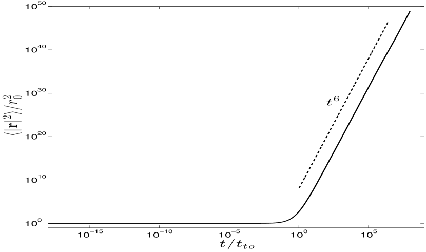
Refer to caption
Figure 1: Monte Carlo results for |𝐫(t)|2delimited-⟨⟩superscript𝐫𝑡2\langle|\mathbf{r}(t)|^{2}\rangle in the power-law diffusion model (157) with S=104𝑆superscript104S=10^{4} and CΔ=1subscript𝐶Δ1C_{\Delta}=1.

On the other, Fig. 2 is a semilog plot of the dispersion compensated by the analytical result (158). It shows that the prefactor is poorly calculated by our Monte Carlo, which gives g6MC26.10approaches-limitsuperscriptsubscript𝑔6𝑀𝐶26.10g_{6}^{MC}\doteq 26.10 and does not appear to converge to the analytical result g6PDsuperscriptsubscript𝑔6𝑃𝐷g_{6}^{PD} as CΔsubscript𝐶ΔC_{\Delta} is decreased.

Refer to caption
Figure 2: Monte Carlo results for |𝐫(t)|2delimited-⟨⟩superscript𝐫𝑡2\langle|\mathbf{r}(t)|^{2}\rangle in the power-law diffusion model (157) with S=104𝑆superscript104S=10^{4} and various CΔsubscript𝐶ΔC_{\Delta}, compensated by the analytical result (158).

Finally, Fig. 3 shows the logarithm of the PDF of pair separations r𝑟r plotted versus r1/3superscript𝑟13r^{1/3} at 141414 different times in the long t6superscript𝑡6t^{6}-range. Self-similarity is well-confirmed by collapse of rescaled curves for different times, but the analytical result (154) is not very accurately reproduced.
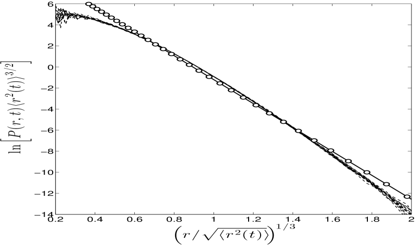
Refer to caption
Figure 3: Logarithm of the rescaled PDF of pair-separations at 141414 different times in the t6superscript𝑡6t^{6} range, for the power-law diffusion model (157). Monte Carlo results for S=105𝑆superscript105S=10^{5} and CΔ=1subscript𝐶Δ1C_{\Delta}=1. The straight line marked with circles (\circ) is the analytical result (154) for d=3𝑑3d=3 and γ=1/3𝛾13\gamma=1/3.

Our conclusion from these exercises is that the adaptive time-stepping scheme should be adequate for exponents of dispersion power-laws, but not for prefactors or PDFs. Since the primary issue in this work is the exponents, we shall employ the adaptive schemes when necessary to cover extensive ranges where constant time-steps are unfeasible. As additional checks on our numerical results for exponents from adaptive schemes, we test for convergence using constants CΔsubscript𝐶ΔC_{\Delta} ranging from 111 to 106.superscript10610^{-6}. We also compare our Monte Carlo results for the diffusion equation with a separate numerical solution of the mean-field equation (128), integrated with a Fortran 90 implementation of the Watt and Shampine RKF45 ODE solver Burkhardt (2012); Shampine et al. (1976). This standard ODE integration method is also adaptive, but with variable time-step determined by preselected error tolerances. We therefore can have confidence that the numerical results for the mean-field theory are well converged.

IV.2 The Inertial-Range Model

We consider first the model (121) obtained for Kolmogorov scaling exponents in the limit L1much-greater-than𝐿1L\gg 1 and thus physically applicable only for separations r𝑟r in the inertial range of scales. This diffusion model applies for both the frozen velocity case and the finite-time correlated case (since β=2/3<1𝛽231\beta=2/3<1). For the purpose of simplifying the numerical work, we opted not to use the exact scaling function J(x)𝐽𝑥J(x) given by integral (97), which in three dimensions yields a complicated expression in terms of generalized hypergeometric functions. Instead, we built a function with the same asymptotic behaviors (98) as the true J(x).𝐽𝑥J(x). We took

J(x)=Jerf(λx)𝐽𝑥subscript𝐽erf𝜆𝑥\displaystyle J(x)=J_{\infty}\mbox{erf}(\lambda x) =\displaystyle= {xx1Jx1cases𝑥much-less-than𝑥1subscript𝐽much-greater-than𝑥1\displaystyle\left\{\begin{array}[]{ll}x&\,\,\,\,\,\,x\ll 1\cr J_{\infty}&\,\,\,\,\,\,x\gg 1\cr\end{array}\right. (161)

with λ=π2J𝜆𝜋2subscript𝐽\lambda=\frac{\sqrt{\pi}}{2J_{\infty}} and J=π2D1(5/3)D1(2/3)0.6396subscript𝐽𝜋2superscriptsubscript𝐷153superscriptsubscript𝐷123approaches-limit0.6396J_{\infty}=\sqrt{\frac{\pi}{2}}\frac{D_{1}^{(5/3)}}{D_{1}^{(2/3)}}\doteq 0.6396. Our expectation was that only these general features should be sufficient to observe the scaling regimes predicted in the previous section. This idea was borne out by the numerical results. In Fig. 4 we plot |𝐫(t)𝐫0|2delimited-⟨⟩superscript𝐫𝑡subscript𝐫02\langle|\mathbf{r}(t)-\mathbf{r}_{0}|^{2}\rangle for the inertial-range diffusion model with r0=1020subscript𝑟0superscript1020r_{0}=10^{-20}. On the same graph we plot for comparison the numerical solution r2(t)r02superscript𝑟2𝑡superscriptsubscript𝑟02r^{2}(t)-r_{0}^{2} of the mean-field equation (128). The two agree very well, and clearly exhibit the four predicted regimes with power-laws t2,t1,t6proportional-toabsentsuperscript𝑡2superscript𝑡1superscript𝑡6\propto t^{2},t^{1},t^{6} and t3,superscript𝑡3t^{3}, successively. A convergence analysis of our adaptive scheme for these results is presented in Appendix A.
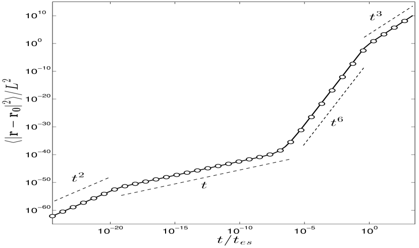
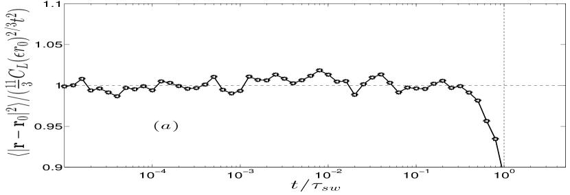
Refer to caption
Figure 4: Numerical results for |𝐫(t)𝐫0|2delimited-⟨⟩superscript𝐫𝑡subscript𝐫02\langle|{\bf r}(t)-{\bf r}_{0}|^{2}\rangle in the inertial-range model (121): Monte Carlo solution of the diffusion equation (\circ) with CΔ=1,S=104formulae-sequencesubscript𝐶Δ1𝑆superscript104C_{\Delta}=1,S=10^{4} and mean-field approximation ().
Refer to caption
Refer to caption
Refer to caption
Refer to caption
Figure 5: Monte Carlo results for |𝐫(t)𝐫0|2,delimited-⟨⟩superscript𝐫𝑡subscript𝐫02\langle|\mathbf{r}(t)-\mathbf{r}_{0}|^{2}\rangle, CΔ=1,subscript𝐶Δ1C_{\Delta}=1, S=104.𝑆superscript104S=10^{4}. Each panel shows the same curves with different scalings. (a) Batchelor regime. (b) Kraichnan regime. (c) t6superscript𝑡6t^{6} regime. (d) Richardson regime. The initial separations are r0/L=105()subscript𝑟0𝐿superscript105r_{0}/L=10^{-5}(\circ), 108()superscript10810^{-8}({\square}) , 1011()superscript101110^{-11}(\triangleright), 1014()superscript101410^{-14}(\triangledown), 1017()superscript101710^{-17}(\diamond), 1020().superscript102010^{-20}(\triangleleft).

To further test the theoretical predictions, we investigate the crossover times between the different regimes and the prefactors of the scaling laws. For example, in Fig. 5(a) we show for various values of r0/Lsubscript𝑟0𝐿r_{0}/L the quantity |𝐫(t)𝐫0|2delimited-⟨⟩superscript𝐫𝑡subscript𝐫02\langle|\mathbf{r}(t)-\mathbf{r}_{0}|^{2}\rangle compensated by the Batchelor-range prediction 113CL(ϵr0)2/3t2113subscript𝐶𝐿superscriptitalic-ϵsubscript𝑟023superscript𝑡2\frac{11}{3}C_{L}(\epsilon r_{0})^{2/3}t^{2} plotted versus the time t/τsw𝑡subscript𝜏𝑠𝑤t/\tau_{sw} rescaled with the sweeping time τsw=r0/v0.subscript𝜏𝑠𝑤subscript𝑟0subscript𝑣0\tau_{sw}=r_{0}/v_{0}. The Batchelor prediction fits the Monte Carlo data to within 0.13%percent0.130.13\% relative error and the end of this regime is very close to t/τsw=1.𝑡subscript𝜏𝑠𝑤1t/\tau_{sw}=1. We similarly show in Fig. 5(b) for the same choices of r0/Lsubscript𝑟0𝐿r_{0}/L the mean-square separation |𝐫(t)𝐫0|2delimited-⟨⟩superscript𝐫𝑡subscript𝐫02\langle|\mathbf{r}(t)-\mathbf{r}_{0}|^{2}\rangle compensated by the Kraichnan-like “diffusive-range” prediction 143CLϵ2/3r05/3t143superscriptsubscript𝐶𝐿superscriptitalic-ϵ23superscriptsubscript𝑟053𝑡\frac{14}{3}C_{L}^{\prime}\epsilon^{2/3}r_{0}^{5/3}t plotted versus t/tto𝑡subscript𝑡𝑡𝑜t/t_{to} with the “takeoff time” ttosubscript𝑡𝑡𝑜t_{to} given by equation (135). The diffusive-range prediction is verified with a 1.8%percent1.81.8\% error and the end of this regime quite convincing scales as 102ttosimilar-toabsentsuperscript102subscript𝑡𝑡𝑜\sim 10^{-2}t_{to}. In Fig. 5(c) we show the corresponding plot of mean-square separation compensated by ε4t6/v06superscript𝜀4superscript𝑡6superscriptsubscript𝑣06\varepsilon^{4}t^{6}/v_{0}^{6} versus t/tto.𝑡subscript𝑡𝑡𝑜t/t_{to}. We see that a t6superscript𝑡6t^{6} range begins at time 102ttosimilar-toabsentsuperscript102subscript𝑡𝑡𝑜\sim 10^{2}t_{to} and extends to the end-of-sweeping time tes=v02/εsubscript𝑡𝑒𝑠superscriptsubscript𝑣02𝜀t_{es}=v_{0}^{2}/\varepsilon with a prefactor g6MC22.96similar-to-or-equalssuperscriptsubscript𝑔6𝑀𝐶22.96g_{6}^{MC}\simeq 22.96 of the t6superscript𝑡6t^{6}-law. This Monte Carlo value lies between the mean-field prediction g6MF55.61approaches-limitsubscriptsuperscript𝑔𝑀𝐹655.61g^{MF}_{6}\doteq 55.61 and the exact power-law diffusion model prediction g6PD15.97,approaches-limitsuperscriptsubscript𝑔6𝑃𝐷15.97g_{6}^{PD}\doteq 15.97, but is quite close to the Monte Carlo result g6PMC26.10approaches-limitsuperscriptsubscript𝑔6𝑃𝑀𝐶26.10g_{6}^{PMC}\doteq 26.10 for the latter model. This suggests that the adaptive time-integration scheme underestimates the effects of diffusion, whereas the true value for the inertial-range model (121) is probably g615.97,approaches-limitsubscript𝑔615.97g_{6}\doteq 15.97, the same as the power-law model (157). It is interesting that the transition between the t1superscript𝑡1t^{1} and t6superscript𝑡6t^{6} scaling ranges is quite broad, covering about four decades. We show finally in Fig. 5(d) the mean-square separation compensated by the Richardson prediction εt3𝜀superscript𝑡3\varepsilon t^{3} plotted versus t/tes.𝑡subscript𝑡𝑒𝑠t/t_{es}. For t>tes𝑡subscript𝑡𝑒𝑠t>t_{es} there is a clear t3superscript𝑡3t^{3} regime with Richardson constant g3MC8.97similar-to-or-equalssuperscriptsubscript𝑔3𝑀𝐶8.97g_{3}^{MC}\simeq 8.97. This constant again lies between mean-field predictions and exact results for a self-similar solution and should not be regarded as accurate. Of course, as emphasized earlier, this entire regime of the inertial-range diffusion model is unphysical and will not be observed in KS model simulations.

IV.3 Comparison with KS Models

Our derivation of diffusion model approximations was sufficiently general that we can consider cases of more direct relevance for KS simulations, with any energy spectrum and without the approximation of large L.𝐿L. Using the formula (109), which is exact for frozen turbulence, one obtains by inverse Fourier transform in 3D that

Dij(𝐫,t)=π2C^ij(𝐤)v0kerf(v0kt2)ei𝐤𝐫d3k.subscript𝐷𝑖𝑗𝐫𝑡𝜋2subscript^𝐶𝑖𝑗𝐤subscript𝑣0𝑘erfsubscript𝑣0𝑘𝑡2superscript𝑒bold-⋅𝑖𝐤𝐫superscript𝑑3𝑘D_{ij}({\bf r},t)=\sqrt{\frac{\pi}{2}}\int\frac{\widehat{C}_{ij}({\bf k})}{v_{0}k}{\rm erf}\left(\frac{v_{0}kt}{\sqrt{2}}\right)e^{i{\bf k}\hbox{\boldmath$\cdot$}{\bf r}}\,d^{3}k. (162)

It is convenient to assume statistical isotropy, so that

C^ij(𝐤)=E(k)4πk2Pij(𝐤),subscript^𝐶𝑖𝑗𝐤𝐸𝑘4𝜋superscript𝑘2subscript𝑃𝑖𝑗𝐤\widehat{C}_{ij}(\mathbf{k})=\frac{E(k)}{4\pi k^{2}}P_{ij}(\mathbf{k}), (163)

where Pij(𝐤)subscript𝑃𝑖𝑗𝐤P_{ij}({\bf k}) is the projection operator onto the subspace orthogonal to 𝐤.𝐤{\bf k}. The trace of the diffusivity tensor becomes

DT(r,t)=2πv00dkkE(k)erf(v0kt2)sin(kr)krsubscript𝐷𝑇𝑟𝑡2𝜋subscript𝑣0superscriptsubscript0𝑑𝑘𝑘𝐸𝑘erfsubscript𝑣0𝑘𝑡2𝑘𝑟𝑘𝑟D_{T}(r,t)=\frac{\sqrt{2\pi}}{v_{0}}\int_{0}^{\infty}\frac{dk}{k}E(k){\rm erf}\left(\frac{v_{0}kt}{\sqrt{2}}\right)\frac{\sin(kr)}{kr} (164)

and DL(r,t)subscript𝐷𝐿𝑟𝑡D_{L}(r,t) can be recovered from

DL(r,t)=1rd0rDT(ρ,t)ρd1𝑑ρ.subscript𝐷𝐿𝑟𝑡1superscript𝑟𝑑superscriptsubscript0𝑟subscript𝐷𝑇𝜌𝑡superscript𝜌𝑑1differential-d𝜌D_{L}(r,t)=\frac{1}{r^{d}}\int_{0}^{r}D_{T}(\rho,t)\,\rho^{d-1}d\rho.

Finally, the diffusivity that appears in equation (90) is

KL(r,t)=2(DL(0,t)DL(r,t)).subscript𝐾𝐿𝑟𝑡2subscript𝐷𝐿0𝑡subscript𝐷𝐿𝑟𝑡K_{L}(r,t)=2(D_{L}(0,t)-D_{L}(r,t)).

To apply these results to the KS models Thomson and Devenish (2005); Osborne et al. (2006); Devenish and Thomson (2009); Nicolleau and Nowakowski (2011), let us recall that those models have a discrete set of wavenumbers distributed as

kn=k1(kNk1)n1N1,subscript𝑘𝑛subscript𝑘1superscriptsubscript𝑘𝑁subscript𝑘1𝑛1𝑁1k_{n}=k_{1}\left(\frac{k_{N}}{k_{1}}\right)^{\frac{n-1}{N-1}}, (165)

for n=1,,N𝑛1𝑁n=1,...,N where k1=2π/Lsubscript𝑘12𝜋𝐿k_{1}=2\pi/L, kN=2π/ηsubscript𝑘𝑁2𝜋𝜂k_{N}=2\pi/\eta and η𝜂\eta is the analogue of the Kolmogorov dissipation length. The energy spectrum generally adopted in these models is

E(k)=CKε2/3n=1Nkn5/3δ(kkn)Δkn𝐸𝑘subscript𝐶𝐾superscript𝜀23superscriptsubscript𝑛1𝑁superscriptsubscript𝑘𝑛53𝛿𝑘subscript𝑘𝑛Δsubscript𝑘𝑛E(k)=C_{K}\varepsilon^{2/3}\sum_{n=1}^{N}k_{n}^{-5/3}\delta(k-k_{n})\Delta k_{n} (166)

where Δkn=(kn+1kn1)/2Δsubscript𝑘𝑛subscript𝑘𝑛1subscript𝑘𝑛12\Delta k_{n}=(k_{n+1}-k_{n-1})/2 and CK=1.5subscript𝐶𝐾1.5C_{K}=1.5 is the Kolmogorov constant, so that CL1.973approaches-limitsubscript𝐶𝐿1.973C_{L}\doteq 1.973 555The standard formula CL=2π(3+α)Γ(2+α)sin(πα/2)CKsubscript𝐶𝐿2𝜋3𝛼Γ2𝛼𝜋𝛼2subscript𝐶𝐾C_{L}=\frac{2\pi}{(3+\alpha)\Gamma(2+\alpha)\sin(\pi\alpha/2)}C_{K} relates the constants CL,CKsubscript𝐶𝐿subscript𝐶𝐾C_{L},C_{K} for a k(1+α)superscript𝑘1𝛼k^{-(1+\alpha)} power-law spectrum; e.g. see Monin and Yaglom (1975), eq.(13.100). This leads to CL1.9727approaches-limitsubscript𝐶𝐿1.9727C_{L}\doteq 1.9727 and CL=CLJ1.262,superscriptsubscript𝐶𝐿subscript𝐶𝐿subscript𝐽approaches-limit1.262C_{L}^{\prime}=C_{L}J_{\infty}\doteq 1.262, the choice of the previous two subsections.. Here ε𝜀\varepsilon is a constant with dimensions of energy dissipation per mass chosen to prescribe values of the rms velocity:

v0=23k1kNE(k)𝑑k.subscript𝑣023superscriptsubscriptsubscript𝑘1subscript𝑘𝑁𝐸𝑘differential-d𝑘v_{0}=\sqrt{\frac{2}{3}\int_{k_{1}}^{k_{N}}E(k)dk}. (167)

The formula (164) with the KS spectrum (166) yields

DT(r,t)=CKϵ2/3v0r2πn=1Nerf(v0knt2)kn11/3sin(knr)Δknsubscript𝐷𝑇𝑟𝑡subscript𝐶𝐾superscriptitalic-ϵ23subscript𝑣0𝑟2𝜋superscriptsubscript𝑛1𝑁erfsubscript𝑣0subscript𝑘𝑛𝑡2superscriptsubscript𝑘𝑛113subscript𝑘𝑛𝑟Δsubscript𝑘𝑛D_{T}(r,t)=\frac{C_{K}\epsilon^{2/3}}{v_{0}r}\sqrt{2\pi}\sum_{n=1}^{N}\frac{\mbox{erf}\left(\frac{v_{0}k_{n}t}{\sqrt{2}}\right)}{k_{n}^{11/3}}\sin\left(k_{n}r\right)\Delta k_{n} (168)

The assumption of isotropy in this formula is only approximately valid for KS simulations. It would be possible to use the general result (162), without assuming isotropy, which would lead to a discrete sum over wavevectors rather than wavevector magnitudes. However, this would make numerical implementation a bit more difficult, without essentially different physics.

We now present simulation results for diffusion models based on Gaussian velocity fields with the spectra of KS models, or, to be brief, “KS diffusion models” . The same Monte Carlo method was employed as for the inertial-range model. In all of our numerical studies we take v0=L=1subscript𝑣0𝐿1v_{0}=L=1. We tried various values for the number of modes N𝑁N and we found that the numerical results on dispersion laws in log-log plots for N100greater-than-or-equivalent-to𝑁100N\gtrsim 100 are not significantly different (see Appendix B). All of our presented results are for N=500,𝑁500N=500, a comparable number to that in the KS studies Thomson and Devenish (2005); Osborne et al. (2006); Devenish and Thomson (2009); Nicolleau and Nowakowski (2011). We have also followed the practice in the KS literature of choosing the smallest length-scale η=r0/10,𝜂subscript𝑟010\eta=r_{0}/10, for initial separation r0.subscript𝑟0r_{0}.

Our first set of numerical experiments investigated whether these more realistic models would exhibit the power-law scaling ranges predicted in section III, with a kN/k1subscript𝑘𝑁subscript𝑘1k_{N}/k_{1} sufficiently large. In Fig. 6 we plot the numerical results for the mean-square separation |𝐫(t)𝐫0|2delimited-⟨⟩superscript𝐫𝑡subscript𝐫02\langle|{\bf r}(t)-{\bf r}_{0}|^{2}\rangle obtained from the KS diffusion model with r0=1020subscript𝑟0superscript1020r_{0}=10^{-20}. We observe very clearly the predicted ranges with power-laws t2,t1,t6superscript𝑡2superscript𝑡1superscript𝑡6t^{2},t^{1},t^{6} and, lastly, the diffusive t1superscript𝑡1t^{1} range at long times expected for a model with finite L.𝐿L. For comparison, we also plot numerical solutions of the mean-field equation (128) using the diffusivity (168). As before, the mean-field theory predictions are quite close to the full Monte Carlo solution of the diffusion model. Lastly, we plot the solution of the mean-field equation for the inertial-range large-L𝐿L diffusivity, with the same choice of constants L,v0𝐿subscript𝑣0L,v_{0} and ε.𝜀\varepsilon. As expected, the dispersion law from this approximation agrees quite well with that of the KS diffusion model for r<L,𝑟𝐿r<L, but predicts a spurious t3superscript𝑡3t^{3} power-law range for r>L.𝑟𝐿r>L. The good agreement justifies a posteriori our simplification of the scaling function J(x)𝐽𝑥J(x) in section IV.2. Our most important general conclusion from this set of experiments is that the KS diffusion models and, we believe, the KS models themselves should exhibit the above four scaling ranges with successive power-laws t2,t1,t6superscript𝑡2superscript𝑡1superscript𝑡6t^{2},t^{1},t^{6} and then t1superscript𝑡1t^{1} again, whenever the scale ratio kN/k1subscript𝑘𝑁subscript𝑘1k_{N}/k_{1} is sufficiently large.

Refer to caption
Figure 6: Numerical results for |𝐫(t)𝐫0|2delimited-⟨⟩superscript𝐫𝑡subscript𝐫02\langle|{\bf r}(t)-{\bf r}_{0}|^{2}\rangle in the KS diffusion model (168), kN/k1=1021subscript𝑘𝑁subscript𝑘1superscript1021k_{N}/k_{1}=10^{21}: Monte Carlo solution of the diffusion equation (\circ) with CΔ=1,S=104formulae-sequencesubscript𝐶Δ1𝑆superscript104C_{\Delta}=1,S=10^{4} and mean-field (). Also MC results (bold-⋯\cdots) for inertial-range model (121).
Refer to caption
Figure 7: Logarithm of the rescaled PDF of pair-separations at 232323 different times in the t6superscript𝑡6t^{6} range, for KS diffusion model with kN/k1=1021subscript𝑘𝑁subscript𝑘1superscript1021k_{N}/k_{1}=10^{21}. Monte Carlo results for S=106𝑆superscript106S=10^{6} and CΔ=1subscript𝐶Δ1C_{\Delta}=1. The straight line marked with circles (\circ) is the analytical result (154) for d=3𝑑3d=3 and γ=1/3𝛾13\gamma=1/3.

In order to discriminate between various alternative theories, it is useful to compare predictions not only for mean-square separations but also for the full probability density P(r,t).𝑃𝑟𝑡P(r,t). Although we do not expect our adaptive time-stepping algorithm to be sufficient to reproduce accurate PDFs, it is still useful to present a few numerical results for the KS diffusion model. In Fig. 7 we plot the Monte Carlo probability distribution calculated for 363636 different times spread within the t6superscript𝑡6t^{6} range. These are rescaled to test for self-similarity and collapse quite well. It should be emphasized that the overall evolution of our IR and KS diffusion models is not self-similar, globally in time. This can be seen most clearly in the existence of time ranges with distinct power-law growth laws, whereas a truly self-similar evolution should have just one power-law. In a sufficiently long t6superscript𝑡6t^{6} range, however, one should expect a self-similar evolution. For example, the inertial-range model (121) in the t6superscript𝑡6t^{6} range reduces to the time-independent diffusivity KL(r,)=CLε2/3r5/3/v0,subscript𝐾𝐿𝑟superscriptsubscript𝐶𝐿superscript𝜀23superscript𝑟53subscript𝑣0K_{L}(r,\infty)=C_{L}^{\prime}\varepsilon^{2/3}r^{5/3}/v_{0}, except for rv0t.much-greater-than𝑟subscript𝑣0𝑡r\gg v_{0}t. Since rv0tsimilar-to𝑟subscript𝑣0𝑡r\sim v_{0}t is nearly the maximum particle separation that can be achieved in the time t,𝑡t, only a very tiny large-r𝑟r tail will experience a different eddy-diffusivity than this. In Fig. 7 we also compare the Monte Carlo results for the KS diffusion model with the exact parameter-free predictions (155),(156) of the power-law diffusion model (152) for d=3𝑑3d=3 and ζ=5/3.𝜁53\zeta=5/3. The agreement is reasonably good. Furthermore, the Monte Carlo results for the KS diffusion model agree almost perfectly with the Monte Carlo results for the power-diffusion model presented in section IV.1. This suggests that if our Monte Carlo could be carried out with a small, constant time-step in a long t6superscript𝑡6t^{6}-range, then the PDF would approach the exact self-similar form of the power-law diffusion model.

We have conjectured that the growth laws of the KS models themselves, asymptotically for kN/k11much-greater-thansubscript𝑘𝑁subscript𝑘11k_{N}/k_{1}\gg 1, are the t2,t1,t6superscript𝑡2superscript𝑡1superscript𝑡6t^{2},t^{1},t^{6} and t1superscript𝑡1t^{1} powers that we have found in the KS diffusion models. How can this be reconciled with the t9/2superscript𝑡92t^{9/2} law predicted in Thomson and Devenish (2005) and verified to greater or lesser extent in subsequent KS simulations Thomson and Devenish (2005); Devenish and Thomson (2009); Nicolleau and Nowakowski (2011)? We argue that the observed t9/2superscript𝑡92t^{9/2} is an artefact of the modest kN/k1subscript𝑘𝑁subscript𝑘1k_{N}/k_{1} ratios achieved in these simulations, which tends to “blend” the distinct scaling ranges, in particular the early-time t1superscript𝑡1t^{1} and t6superscript𝑡6t^{6} ranges, between which lies a broad transition zone. In support of this argument, we have performed a sequence of Monte Carlo simulations of the KS diffusion model with scale ratios kN/k1=103,104,105,106subscript𝑘𝑁subscript𝑘1superscript103superscript104superscript105superscript106k_{N}/k_{1}=10^{3},10^{4},10^{5},10^{6}. The last ratio is chosen to correspond roughly to that employed in the previous KS simulations Thomson and Devenish (2005); Devenish and Thomson (2009); Nicolleau and Nowakowski (2011). Because the range of time-scales is not so great, we have been able to carry out the time-integration not only with the adaptive algorithm employed up until now, but also with a constant time step Δt=0.1ηv0Δ𝑡0.1𝜂subscript𝑣0\Delta t=0.1\frac{\eta}{v_{0}} which resolves the effects of even the smallest eddies, equivalent to that used in recent KS simulations Devenish and Thomson (2009); Nicolleau and Nowakowski (2011). The results of the two time-advancement schemes for the dispersion curves are identical when plotted in log-log. As illustrated in Fig. 8, a t9/2superscript𝑡92t^{9/2} regime seems to appear as we increase the ratio kN/k1.subscript𝑘𝑁subscript𝑘1k_{N}/k_{1}. This figure should be compared with Fig. 2 of Devenish and Thomson (2009) and Fig. 1 of Nicolleau and Nowakowski (2011), which it matches very closely. Although we see a similar “t9/2superscript𝑡92t^{9/2}-range” at the values of kN/k1subscript𝑘𝑁subscript𝑘1k_{N}/k_{1} used in previous KS simulations, covering 1-2 decades in time, it is clear from our results in Fig. 6 that this is only a transitional regime of the KS diffusion model. In fact, for the case kN/k1=106subscript𝑘𝑁subscript𝑘1superscript106k_{N}/k_{1}=10^{6} which shows the long “t9/2superscript𝑡92t^{9/2}-range” we find tto102approaches-limitsubscript𝑡𝑡𝑜superscript102t_{to}\doteq 10^{-2} and thus the broad transition zone between the t1superscript𝑡1t^{1} and t6superscript𝑡6t^{6} laws covers the interval from 104superscript10410^{-4} to 100.superscript10010^{0}. This includes all of the apparent “t9/2superscript𝑡92t^{9/2}-range”. If we go to kN/k1=108,subscript𝑘𝑁subscript𝑘1superscript108k_{N}/k_{1}=10^{8}, the power-law steepens into a t5superscript𝑡5t^{5}-law. At still larger values of kN/k1subscript𝑘𝑁subscript𝑘1k_{N}/k_{1} four asymptotic scaling ranges emerge, with distinct power-law scalings of t2,t1,t6superscript𝑡2superscript𝑡1superscript𝑡6t^{2},t^{1},t^{6} and t1.superscript𝑡1t^{1}. We expect that the same is true of the KS models themselves at sufficiently large kN/k1.subscript𝑘𝑁subscript𝑘1k_{N}/k_{1}.
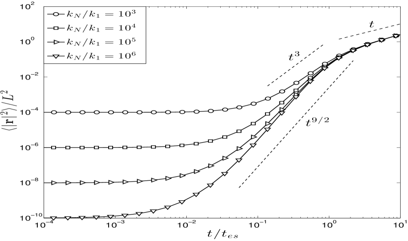
Refer to caption
Figure 8: Monte Carlo results for |𝐫(t)|2delimited-⟨⟩superscript𝐫𝑡2\langle|\mathbf{r}(t)|^{2}\rangle in KS diffusion model for various values of kN/k1subscript𝑘𝑁subscript𝑘1k_{N}/k_{1}, with Δt=0.1rv0Δ𝑡0.1𝑟subscript𝑣0\Delta t=0.1\frac{r}{v_{0}}, S=104𝑆superscript104S=10^{4}.

Finally, we note that for kN/k1<104,subscript𝑘𝑁subscript𝑘1superscript104k_{N}/k_{1}<10^{4}, the short range of superdiffusive growth of dispersion approximates a t3superscript𝑡3t^{3}-law. This agrees with the observations of Osborne et al. (2006); Nicolleau and Nowakowski (2011) for KS models. Note, however, that the physics is completely different from turbulent Richardson diffusion, which would allow t3superscript𝑡3t^{3} ranges of arbitrary extent. In fact, the narrow range of such a power-law in our KS diffusion model arises only because of the “merging” of many distinct ranges. In particular, the exponent of the apparent power-law must decrease with decreasing kN/k1subscript𝑘𝑁subscript𝑘1k_{N}/k_{1} to match the t1superscript𝑡1t^{1}-law starting at r=L,𝑟𝐿r=L, until finally the superdiffusive range disappears entirely when kN/k11.subscript𝑘𝑁subscript𝑘11k_{N}/k_{1}\approx 1.

V Conclusions

We have derived in this paper a diffusion equation for particle-pair dispersion in synthetic Eulerian turbulence modelled by Gaussian velocity ensembles. The main analytical result is the formula (84) for the 222-particle diffusivity and its special cases (96) for frozen velocities and (109) for finite time-correlated velocities. Although the description of pair-dispersion as a diffusion process is not exact (except in certain limiting cases), it arises from a well-motivated set of analytical approximations. Our results confirm the physical argument of Thomson & Devenish Thomson and Devenish (2005) that pair-dispersion in such models is fundamentally altered by sweeping decorrelation effects, not experienced by particle pairs in hydrodynamic turbulence. Thus, the t3superscript𝑡3t^{3}-law observed in previous simulations with synthetic turbulence Elliott, Jr. and Majda (1996); Fung and Vassilicos (1998); Malik and Vassilicos (1999); Dávila and Vassilicos (2003); Nicolleau and Yu (2004) is quite likely an artefact either of the numerical approximations employed or of the shortness of the inertial ranges. However, we argue as well for a similar origin of the t9/2superscript𝑡92t^{9/2}-law proposed by Thomson & Devenish Thomson and Devenish (2005) for synthetic turbulence ensembles with zero mean velocities. Solutions of our diffusion model for such ensembles at Reynolds numbers comparable to those employed in KS simulations that show a t9/2superscript𝑡92t^{9/2}-law range reproduce that finding, but our model yields instead distinct t2,t1,t6superscript𝑡2superscript𝑡1superscript𝑡6t^{2},t^{1},t^{6} and t1superscript𝑡1t^{1}-ranges at higher Reynolds numbers. We thus argue that the asymptotic high Reynolds-number behavior of particle dispersion in synthetic Eulerian turbulence with zero mean-velocities is the same as that predicted by Thomson & Devenish Thomson and Devenish (2005) for ensembles with large mean velocities.

Synthetic models of turbulence such as Kinematic Simulations have been used to investigate turbulent transport of passive objects (particles, lines, etc.) in such varied problems as environmental flow, aeroacoustics, kinematic magnetic dynamo, and superfluids Baggaleyetal09; Nicolleauetal11. However, such numerical studies must clearly be employed with utmost caution, especially to derive conclusions about turbulent transport at very high Reynolds numbers. The difference in sweeping effects in synthetic Eulerian turbulence and in real hydrodynamic turbulence imply not only quantitatively different scaling laws but also substantially different physics.

Acknowledgements.
The work of GE was partially supported by the NSF Grant CMMI-0941530 at Johns Hopkins University.

Appendix A Monte Carlo Time-Step

We tested the dependence of the log-log plots of dispersion on the value of CΔsubscript𝐶ΔC_{\Delta}. We plot in Fig. 9 the Monte Carlo results for values of CΔsubscript𝐶ΔC_{\Delta} ranging from 111 to 106superscript10610^{-6}. There is no observable change in the behavior.

Appendix B Number of Fourier Modes

We also tested the dependence of our dispersion results for the KS diffusion models on the number of Fourier modes N𝑁N. We show in Fig. 10 log-log plots of the dispersion curves for different values of N,𝑁N, obtained from Monte Carlo calculations with CΔ=1subscript𝐶Δ1C_{\Delta}=1 and S=104𝑆superscript104S=10^{4}. The results are nearly indistinguishable for N100greater-than-or-equivalent-to𝑁100N\gtrsim 100. All of our simulations in the text used N=500𝑁500N=500.

Refer to caption
Figure 9: Monte Carlo results for |𝐫(t)𝐫0|2delimited-⟨⟩superscript𝐫𝑡subscript𝐫02\langle|\mathbf{r}(t)-\mathbf{r}_{0}|^{2}\rangle in the inertial-range diffusion model calculated with S=102𝑆superscript102S=10^{2} samples and varying CΔ=1subscript𝐶Δ1C_{\Delta}=1 to CΔ=106.subscript𝐶Δsuperscript106C_{\Delta}=10^{-6}.
Refer to caption
Figure 10: Monte Carlo results for |𝐫(t)𝐫0|2delimited-⟨⟩superscript𝐫𝑡subscript𝐫02\langle|\mathbf{r}(t)-\mathbf{r}_{0}|^{2}\rangle in the KS diffusion model calculated with CΔ=1,subscript𝐶Δ1C_{\Delta}=1, S=104𝑆superscript104S=10^{4} samples, varying number of Fourier modes from N=10𝑁10N=10 to N=104.𝑁superscript104N=10^{4}.

References

  • Richardson (1926) L. F. Richardson, Proc. R. Soc. London, Ser. A 110, 709 (1926).
  • Elliott, Jr. and Majda (1996) F. W. Elliott, Jr. and A. J. Majda, Phys. Fluids 8, 1052 (1996).
  • Fung and Vassilicos (1998) J. C. H. Fung and J. C. Vassilicos, Phys. Rev. E 57, 1677 (1998).
  • Malik and Vassilicos (1999) N. A. Malik and J. C. Vassilicos, Phys. Fluids 11, 1572 (1999).
  • Dávila and Vassilicos (2003) J. Dávila and J. C. Vassilicos, Phys. Rev. Lett. 91, 144501 (2003).
  • Nicolleau and Yu (2004) F. Nicolleau and G. Yu, Phys. Fluids 16, 2309 (2004).
  • Chaves et al. (2003) M. Chaves, K. Gawȩdzki, P. Horvai, A. Kupiainen, and M. Vergassola, J. Stat. Phys. 113, 643 (2003).
  • Thomson and Devenish (2005) D. J. Thomson and B. J. Devenish, J. Fluid Mech. 526, 277 (2005).
  • Osborne et al. (2006) D. R. Osborne, J. C. Vassilicos, K. Sung, and J. D. Haigh, Phys. Rev. E 74, 036309 (2006).
  • Devenish and Thomson (2009) B. J. Devenish and D. J. Thomson, Phys. Rev. E 80, 048301 (2009).
  • Nicolleau and Nowakowski (2011) F. C. G. A. Nicolleau and A. F. Nowakowski, Phys. Rev. E 83, 056317 (2011).
  • Eyink and Xin (2000) G. L. Eyink and J. Xin, J. Stat.Phys. 100, 679 (2000).
  • Frisch (1995) U. Frisch, Turbulence. The Legacy of A. N. Kolmogorov (Cambridge University Press, 1995).
  • Kraichnan (1968) R. H. Kraichnan, Phys. Fluids 11, 945 (1968).
  • Falkovich et al. (2001) G. Falkovich, K. Gawȩdzki, and M. Vergassola, Rev. Mod. Phys. 73, 913 (2001).
  • Balk (2002) A. M. Balk, J. Fluid Mech. 467, 163 (2002).
  • Kraichnan (1966) R. H. Kraichnan, Phys. Fluids 9, 1937 (1966).
  • Lundgren (1981) T. S. Lundgren, J. Fluid Mech. 111, 27 (1981).
  • Eyink (2012) G. L. Eyink, The diffusion approximation in turbulent particle dispersion (2012), preprint.
  • Monin and Yaglom (1975) A. S. Monin and A. M. Yaglom, Statistical Fluid Mechanics, vol. II (MIT Press, 1975).
  • Bernard et al. (1998) D. Bernard, K. Gawȩdzki, and A. Kupiainen, J. Stat. Phys. 90, 519 (1998).
  • Batchelor (1950) G. K. Batchelor, Quarterly Journal of the Royal Meteorological Society 76, 133 (1950).
  • Batchelor (1952) G. K. Batchelor, Mathematical Proceedings of the Cambridge Philosophical Society 48, 345 (1952).
  • Eyink (2011) G. L. Eyink, Phys. Rev. E 83, 056405 (2011).
  • Chen and Kraichnan (1998) S. Chen and R. H. Kraichnan, Physics of Fluids 10, 2867 (1998).
  • Frisch and Wirth (1996) U. Frisch and A. Wirth, EPL (Europhysics Letters) 35, 683 (1996).
  • Taylor (1921) G. I. Taylor, Proceedings of the London Mathematical Society s2-20, 196 (1921).
  • Burkhardt (2012) J. Burkhardt (2012), Florida State University website, http://people.sc.fsu.edu/similar-to\simjburkardt/f_src/rkf45.
  • Shampine et al. (1976) L. Shampine, H. Watts, and S. Davenport, SIAM Review 18, 376 (1976).