Searching for gravitational waves from binary coalescence

Abstract

We describe the implementation of a search for gravitational waves from compact binary coalescences in LIGO and Virgo data. This all-sky, all-time, multi-detector search for binary coalescence has been used to search data taken in recent LIGO and Virgo runs. The search is built around a matched filter analysis of the data, augmented by numerous signal consistency tests designed to distinguish artifacts of non-Gaussian detector noise from potential detections. We demonstrate the search performance using Gaussian noise and data from the fifth LIGO science run and demonstrate that the signal consistency tests are capable of mitigating the effect of non-Gaussian noise and providing a sensitivity comparable to that achieved in Gaussian noise.

I Introduction

Coalescing binaries of compact objects such as neutron stars and stellar-mass black holes are promising gravitational-wave (GW) sources for ground-based, kilometer-scale interferometric detectors such as LIGO Abbott et al. (2009a), Virgo Accadia et al. (2012), and GEO600 Grote (2008), which are sensitive to waves of frequencies between tens and thousands of Hertz. Numerous searches for these signals were performed on data from the six LIGO and GEO science runs (S1–S6) and from the four Virgo science runs (VSR1–4) Abbott et al. (2004, 2005a, 2006a, 2005b, 2006b, 2008a, 2008b, 2009b, 2009c); Abadie et al. (2010a, 2012a).

Over time, the software developed to run these searches and evaluate the significance of results evolved into a sophisticated pipeline, known as ihope. An early version of the pipeline was described in Brown (2005). In this paper, we describe the ihope pipeline in detail and we characterize its detection performance by comparing the analysis of a month of real data with the analysis of an equivalent length of simulated data with Gaussian stationary noise.

Compact binary coalescences (CBCs) consist of three dynamical phases: a gradual inspiral, which is described accurately by the post-Newtonian approximation to the Einstein equations Blanchet (2002); a nonlinear merger, which can be modeled with numerical simulations (see Centrella et al. (2010); Hannam (2009); Sperhake et al. (2011) for recent reviews); and the final ringdown of the merged object to a quiescent state Berti et al. (2007). For the lighter NS–NS systems, only the inspiral lies within the band of detector sensitivity. Since Compact binary coalescence (CBC) waveforms are well modeled, it is natural to search for them by matched-filtering the data with banks of theoretical template waveforms Wainstein and Zubakov (1962).

The most general CBC waveform is described by seventeen parameters, which include the masses and intrinsic spins of the binary components, as well as the location, orientation, and orbital elements of the binary. It is not feasible to perform a search by placing templates across such a high-dimensional parameter space. However, it is astrophysically reasonable to neglect orbital eccentricity Cokelaer and Pathak (2009); Brown and Zimmerman (2010); furthermore, CBC waveforms that omit the effects of spins have been shown to have acceptable phase overlaps with spinning-binary waveforms, and are therefore suitable for the purpose of detecting CBCs, if not to estimate their parameters accurately Van Den Broeck et al. (2009).

Thus, CBC searches so far have relied on nonspinning waveforms that are parameterized only by the component masses, by the location and orientation of the binary, by the initial orbital phase, and by the time of coalescence. Among these parameters, the masses determine the intrinsic phasing of the waveforms, while the others affect only the relative amplitudes, phases, and timing observed at multiple detector sites Allen et al. (2012). It follows that templates need to be placed only across the two-dimensional parameter space spanned by the masses Allen et al. (2012). Even so, past CBC searches have required many thousands of templates to cover their target ranges of masses. (We note that ihope could be extended easily to nonprecessing binaries with aligned spins. However, more general precessing waveforms would prove more difficult, as discussed in Apostolatos et al. (1994); Apostolatos (1995); Buonanno et al. (2003); Pan et al. (2004).)

In the context of stationary Gaussian noise, matched-filtering would directly yield the most statistically significant detection candidates. In practice, environmental and instrumental disturbances cause non-Gaussian noise transients (glitches) in the data. Searches must distinguish between the candidates, or triggers, resulting from glitches and those resulting from true GWs. The techniques developed for this challenging task include coincidence (signals must be observed in two or more detectors with consistent mass parameters and times of arrival), signal-consistency tests (which quantify how much a signal’s amplitude and frequency evolution is consistent with theoretical waveforms Allen (2005)), and data quality vetoes (which identify time periods when the detector glitch rate is elevated). We describe these in detail later.

The statistical significance after the consistency tests have been applied is then quantified by computing the false alarm probability (FAP) or false alarm rate (FAR) of each candidate; we define both below. For this, the background of noise-induced candidates is estimated by performing time shifts, whereby the coincidence and consistency tests are run after imposing relative time offsets on the data from different detectors. Any consistent candidate found in this way must be due to noise; furthermore, if the noise of different detectors is uncorrelated, the resulting background rate is representative of the rate at zero shift.

The sensitivity of the search to CBC waves is estimated by adding simulated signals (injections) to the detector data, and verifying which are detected by the pipeline. With this diagnostic we can tune the search to a specific class of signals (e.g., a region in the mass plane), and we can give an astrophysical interpretation, such as an upper limit on CBC rates Brady and Fairhurst (2008), to completed searches.

As discussed below, commissioning a GW search with the ihope pipeline requires a number of parameter tunings, which include the handling of coincidences, the signal-consistency tests, and the final ranking of triggers. To avoid biasing the results, ihope permits a blind analysis: the results of the non-time-shifted analysis can be sequestered, and tuning performed using only the injections and time-shifted results. Later, with the parameter tunings frozen, the non-time-shifted results can be unblinded to reveal the candidate GW events.

This paper is organized as follows. In Sec. II we provide a brief overview of the ihope pipeline, and describe its first few stages (data conditioning, template placement, filtering, coincidence), which would be sufficient to implement a search in Gaussian noise but not, as we show, in real detector data. In Sec. III we describe the various techniques that have been developed to eliminate the majority of background triggers due to non-Gaussian noise. In Sec. IV we describe how the ihope results are used to make astrophysical statements about the presence or absence of signals in the data, and to put constraints on CBC event rates. Last, in Sec. V we discuss ways in which the analysis can be enhanced to improve sensitivity, reduce latency, and find use in the advanced-detector era.

Throughout this paper we show representative ihope output, taken from a search of one month of LIGO data from the S5 run (the third month in Abbott et al. (2009c)), when all three LIGO detectors (but not Virgo) were operational. The search focused on low-mass CBC signals with component masses $>1\,M_{\odot}$ and total mass $<25\,M_{\odot}$. For comparison, we also run the same search on Gaussian noise generated at the design sensitivity of the Laser Interferometer Gravitational-wave Observatory (LIGO) detectors (using the same data times as the real data). Where we perform GW-signal injections (see Sec. IV.3), we adopt a population of binary-neutron-star inspirals, uniformly distributed in distance, coalescence time, sky position and orientation angles.

II IHOPE, part 1: setting up a matched-filtering search with multiple-detector coincidence

The stages of the ihope pipeline are presented schematically in Fig. 1, and are described in detail in Secs. II–IV of this paper. First, the science data to be analyzed is identified and split into $2048\text{\,}\mathrm{s}$ blocks, and the power spectral density is estimated for each block (see Sec. II.1). Next, a template bank is constructed independently for each detector and each block (Sec. II.2). The data blocks are matched-filtered against each bank template, and the times when the signal-to-noise ratio (SNR) rises above a set threshold are recorded as triggers (Sec. II.3). The triggers from each detector are then compared to identify coincidences—that is, triggers that occur in two or more detectors with similar masses and compatible times (Sec. II.4).

Figure 1: Structure of the ihope pipeline.

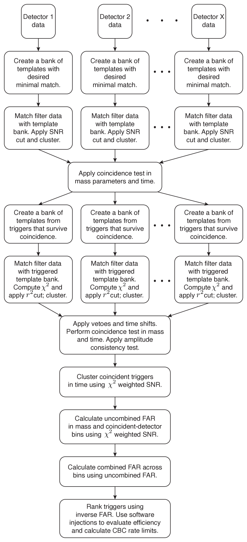
If detector noise was Gaussian and stationary, we could proceed directly to the statistical interpretation of the triggers. Unfortunately, non-Gaussian noise glitches generate both an increase in the number of low-SNR triggers as well as high-SNR triggers that form long tails in the distribution of SNRs. The increase in low-SNR triggers will cause an small, but inevitable, reduction in the sensitivity of the search. It is, however, vital to distinguish the high-SNR background triggers from those caused by real GW signals. To achieve this, the coincident triggers are used to generate a reduced template bank for a second round of matched-filtering in each detector (see the beginning of Sec. III). This time, signal-consistency tests are performed on each trigger to help differentiate background from true signals (Secs. III.1, III.2). These tests are computationally expensive, so we reserve them for this second pass. Single-detector triggers are again compared for coincidence, and the final list is clustered and ranked (Sec. III.5), taking into account signal consistency, amplitude consistency among detectors (Sec. III.3), as well as the times in which the detectors were not operating optimally (Sec. III.4). These steps leave coincident triggers that have a quasi-Gaussian distribution; they can now be evaluated for statistical significance, and used to derive event-rate upper limits in the absence of a detection.

To do this, the steps of the search that involve coincidence are repeated many times, artificially shifting the time stamps of triggers in different detectors, such that no true GW signal would actually be found in coincidence (Sec. IV.1). The resulting time-shift triggers are used to calculate the FAR of the in-time (zero-shift) triggers. Those with FAR lower than some threshold are the GW-signal candidates (Sec. IV.2). Simulated GW signals are then injected into the data, and by observing which injections are recovered as triggers with FAR lower than some threshold, we can characterize detection efficiency as a function of distance and other parameters (Sec. IV.3), providing an astrophysical interpretation for the search. Together with the FARs of the loudest triggers, the efficiency yields the upper limits (Sec. IV.4).

II.1 Data segmentation and conditioning, power-spectral-density generation

As a first step in the pipeline, ihope identifies the stretches of detector data that should be analyzed: for each detector, such science segments are those for which the detector was locked (i.e., interferometer laser light was resonant in Fabry–Perot cavities Abbott et al. (2009a)), no other experimental work was being performed, and the detector’s “science mode” was confirmed by a human “science monitor.” ihope builds a list of science-segment times by querying a network-accessible database that contains this information for all detectors.

The LIGO and Virgo GW-strain data are sampled at $16,384\text{\,}\mathrm{Hz}$ and $20,000\text{\,}\mathrm{Hz}$, respectively, but both are down-sampled to $4096\text{\,}\mathrm{Hz}$ prior to analysis Brown (2005), since at frequencies above $1\text{\,}\mathrm{kHz}$ to $2\text{\,}\mathrm{kHz}$ detector noise overwhelms any likely CBC signal. This sampling rate sets the Nyquist frequency at $2048\text{\,}\mathrm{Hz}$; to prevent aliasing, the data are preconditioned with a time-domain digital filter with low-pass cutoff at the Nyquist frequency Brown (2005). While CBC signals extend to arbitrarily low frequencies, detector sensitivity degrades rapidly, so very little GW power could be observed below $40\text{\,}\mathrm{Hz}$. Therefore, we usually suppress signals below $30\text{\,}\mathrm{Hz}$ with two rounds of 8th-order Butterworth high-pass filters, and analyze data only above $40\text{\,}\mathrm{Hz}$.

Both the low- and high-pass filters corrupt the data at the start and end of a science segment, so the first and last few seconds of data (typically $8\text{\,}\mathrm{s}$) are discarded after applying the filters. Furthermore, SNRs are computed by correlating templates with the (noise-weighted) data stream, which is only possible if a stretch of data of at least the same length as the template is available. Altogether, the data are split into $256\text{\,}\mathrm{s}$ segments, and the first and last $64\text{\,}\mathrm{s}$ of each segment are not used in the search. Neighboring segments are overlapped by $128\text{\,}\mathrm{s}$ to ensure that all available data are analyzed.

The strain power spectral density (PSD) is computed separately for every $2048\text{\,}\mathrm{s}$ block of data (consisting of 15 overlapping $256\text{\,}\mathrm{s}$ segments). The blocks themselves are overlapped by $128\text{\,}\mathrm{s}$. The block PSD is estimated by taking the median Brown (2004) (in each frequency bin) of the segment PSDs, ensuring robustness against noise transients and GW signals (whether real or simulated). The PSD is used in the computation of SNRs, and to set the spacing of templates in the banks. Science segments shorter than $2064\text{\,}\mathrm{s}$ ($2048\text{\,}\mathrm{s}$ block length and $16\text{\,}\mathrm{s}$ to account for the padding on either side) are not used in the analysis, since they cannot provide an accurate PSD estimate.

II.2 Template-bank generation

Template banks must be sufficiently dense in parameter space to ensure a minimal loss of matched-filtering SNR for any CBC signal within the mass range of interest; however, the computational cost of a search is proportional to the number of templates in a bank. The method used to place templates must balance these considerations. This problem is well explored for nonspinning CBC signals Cokelaer (2007); Babak et al. (2006); Owen and Sathyaprakash (1999); Owen (1996); Balasubramanian et al. (1996); Dhurandhar and Sathyaprakash (1994); Sathyaprakash and Dhurandhar (1991), for which templates need only be placed across the two-dimensional intrinsic-parameter space spanned by the two component masses. The other extrinsic parameters enter only as amplitude scalings or phase offsets, and the SNR can be maximized analytically over these parameters after filtering by each template.

Templates are placed in parameter space so that the match between any GW signal and the best-fitting template is better than a minimum match MM (typically 97%). The match between signals $h$ with parameter vectors $\boldsymbol{\xi}_{1}$ and $\boldsymbol{\xi}_{2}$ is defined as

$$\max_{t_{c},\phi_{c}}\frac{\bigl{(}h(\boldsymbol{\xi}_{1})\big{|}h(\boldsymbol{\xi}_{2})\bigr{)}}{\sqrt{\bigl{(}h(\boldsymbol{\xi}_{1})\big{|}h(\boldsymbol{\xi}_{1})\bigr{)}}\sqrt{\bigl{(}h(\boldsymbol{\xi}_{2})\big{|}h(\boldsymbol{\xi}_{2})\bigr{)}}}$$ (1)

where $t_{c}$ and $\phi_{c}$ are the time and phase of coalescence of the signal, $(\cdot|\cdot)$ is the standard noise-weighted inner product

$$(a|b)=4\,\mathrm{Re}\int_{f_{\mathrm{low}}}^{f_{\mathrm{high}}}\frac{\tilde{a}^{*}(f)\,\tilde{b}(f)}{S_{n}(f)}df,$$ (2)

with $S_{n}(f)$ the one-sided detector-noise PSD. The MM represents the worst-case reduction in matched-filtering SNR, and correspondingly the worst-case reduction in the maximum detection distance of a search. Thus, under the assumption of sources uniformly distributed in volume, the loss in sensitivity due to template-bank discreteness is bounded by $\mathrm{MM}^{3}$, or $\simeq 10\%$ for $\mathrm{MM}=97\%$.

It is computationally expensive to obtain template mismatches for pairs of templates using Eq. (2), so an approximation based on a parameter-space metric is used instead:

$$1-(h(\boldsymbol{\xi})|h(\boldsymbol{\xi}+\delta\boldsymbol{\xi}))\simeq\sum_{ij}g_{ij}(\boldsymbol{\xi})\,\delta\xi^{i}\,\delta\xi^{j},$$ (3)

where

$$g_{ij}(\boldsymbol{\xi})=-\frac{1}{2}\frac{\partial^{2}\left(h(\boldsymbol{\xi})|h(\boldsymbol{\xi})\right)}{\partial\xi^{i}\partial\xi^{j}}.$$ (4)

The approximation holds as long as the metric is roughly constant between bank templates, and is helped by choosing parameters (i.e., coordinates $\boldsymbol{\xi}$) that make the metric almost flat, such as the “chirp times” $\tau_{0}$, $\tau_{3}$ given by Sathyaprakash (1994)

$$\tau_{0} = \frac{5}{256\pi f_{\mathrm{low}}\eta}\left(\frac{\pi GMf_{\mathrm{low}}}{c^{3}}\right)^{-5/3},$$ (5)

$$\tau_{3} = \frac{5}{8f_{\mathrm{low}}\eta}\left(\frac{\pi GMf_{\mathrm{low}}}{c^{3}}\right)^{-2/3}.$$ (6)

Here $M$ is the total mass, $\eta$ is the symmetric mass ratio $\eta=m_{1}m_{2}/M^{2}$ and $f_{\mathrm{low}}$ is the lower frequency cutoff used in the template generation.

For the S5–S6 and VSR1–3 CBC searches, templates were placed on a regular hexagonal lattice in $\tau_{0}$–$\tau_{3}$ space Cokelaer (2007), sized so that MM would be 97% Abbott et al. (2009b, c); Abadie et al. (2012a). The metric was computed using inspiral waveforms at the second post-Newtonian (2PN) order in phase. Higher-order templates are now used in searches (some including merger and ringdown), but not for template placement; work is ongoing to implement that. Figure 2 shows a typical template bank in both $m_{1}$–$m_{2}$ and $\tau_{0}$–$\tau_{3}$ space for the low-mass CBC search. For a typical data block, the bank contains around 6000 templates (Virgo, which has a a flatter noise PSD, requires more).

Figure 2: A typical template bank for a low-mass CBC inspiral search, as plotted in $m_{1}$–$m_{2}$ space (top panel) and $\tau_{0}$–$\tau_{3}$ space (bottom panel). Templates are distributed more evenly over $\tau_{0}$ and $\tau_{3}$, since the parameter-space metric is approximately flat in those coordinates.

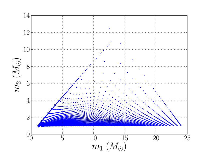
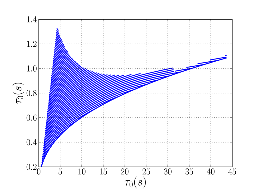
As Eqs. (4) and (2) imply, the metric depends on both the detector-noise PSD and the frequency limits $f_{\mathrm{low}}$ and $f_{\mathrm{high}}$. We set $f_{\mathrm{low}}$ to $40\text{\,}\mathrm{Hz}$, while $f_{\mathrm{high}}$ is chosen naturally as the frequency at which waveforms end ($200\text{\,}\mathrm{Hz}$ and $2\text{\,}\mathrm{kHz}$ for the highest- and lowest-mass signals, respectively). The PSD changes between data blocks, but usually only slightly, so template banks stay roughly constant over time in a data set.

II.3 Matched filtering

The central stage of the pipeline is the matched filtering of detector data with bank templates, resulting in a list of triggers that are further analyzed downstream. This stage was described in detail in Ref. Brown (2004); here we sketch its key features.

The waveform from a non-spinning CBC, as observed by a ground-based detector and neglecting higher-order amplitude corrections, can be written as

$$h(\tau)=h_{0}(\tau)\cos\Phi_{0}+h_{\pi/2}(\tau)\sin\Phi_{0},$$ (7)

with

$$\left(\begin{array}[]{c}h_{0}(\tau)\\ h_{\pi/2}(\tau)\end{array}\right)=Af(\tau)^{2/3}\left(\begin{array}[]{c}\cos\bigl{(}\Phi(\tau)\bigr{)}\\ -\sin\bigl{(}\Phi(\tau)\bigr{)}\end{array}\right).$$ (8)

Here, $\tau$ is a time variable relative to the coalescence time, $t_{c}$. The constant amplitude $A$ and phase $\Phi_{0}$, between them, depend on all the binary parameters: masses, sky location and distance, orientation, and (nominal) orbital phase at coalescence. By contrast, the time-dependent frequency $f(\tau)$ and phase $\Phi(\tau)$ depend only on the component masses and on the absolute time of coalescence.

The squared SNR $\rho^{2}$ for the data $s$ and template $h$, analytically maximized over $A$ and $\Phi_{0}$, is given by

$$\rho^{2}=\frac{(s|h_{0})^{2}+(s|h_{\pi/2})^{2}}{(h_{0}|h_{0})};$$ (9)

here we assume that $\tilde{h}_{\pi/2}(f)=i\tilde{h}_{0}(f)$, which is identically true for waveforms defined in the frequency domain with the stationary-phase approximation Droz et al. (1999), and approximately true for all slowly evolving CBC waveforms.

The maximized statistic $\rho^{2}$ of Eq. (9) is a function only of the component masses and the time of coalescence $t_{c}$. Now, a time shift can be folded in the computation of inner products by noting that $g(\tau)=h(\tau-\Delta t_{c})$ transforms to $\tilde{g}(f)=e^{i2\pi f\Delta t_{c}}\tilde{h}(f)$; therefore, the SNR can be computed as a function of $t_{c}$ by the inverse Fourier transform (a complex quantity)

$$(s|h)(\Delta t_{c})=4\int_{f_{\mathrm{low}}}^{f_{\mathrm{high}}}\frac{\tilde{s}(f)\tilde{h}^{*}(f)}{S_{n}(f)}e^{2\pi if\Delta t_{c}}df.$$ (10)

Furthermore, if $\tilde{h}_{\pi/2}(f)=i\tilde{h}_{0}(f)$ then Eq. (10), computed for $h=h_{0}$, yields $(s|h_{0})(\Delta t_{c})+i\,(s|h_{\pi/2})(\Delta t_{c})$.

The ihope matched-filtering engine implements the discrete analogs of Eqs. (9) and (10) Allen et al. (2012) using the efficient FFTW library FFT . The resulting SNRs are not stored for every template and every possible $t_{c}$; instead, we only retain triggers that exceed an empirically determined threshold (typically 5.5), and that corresponds to maxima of the SNR time series—that is, a trigger above the threshold is kept only if there are no triggers with higher SNR within a predefined time window, typically set to the length of the template (this is referred to as time clustering).

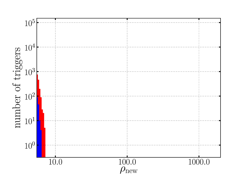
For a single template and time and for detector data consisting of Gaussian noise, $\rho^{2}$ follows a $\chi^{2}$ distribution with two degrees of freedom, which makes a threshold of 5.5 seem rather large: $p(\rho>5.5)=2.7\times 10^{-7}$. However, we must account for the fact that we consider a full template bank and maximize over time of coalescence: the bank makes for, conservatively, a thousand independent trials at any point in time, while trials separated by 0.1 seconds in time are essentially independent. Therefore, we expect to see a few triggers above this threshold already in a few hundred seconds of Gaussian noise, and a large number in a year of observing time. Furthermore, since the data contain many non-Gaussian noise transients, the trigger rate will be even higher. In Fig. 3 we show the distribution of triggers as a function of SNR in a month of simulated Gaussian noise (blue) and real data (red) from LIGO’s fifth science run (S5). The difference between the two is clearly noticeable, with a tail of high SNR triggers extending to SNRs well over 1000 in real data.

Figure 3: Distribution of single detector trigger SNRs in a month of simulated Gaussian noise (blue) and real S5 LIGO data (red) from the Hanford interferometer H1.

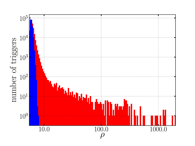
It is useful to not just cluster in time, but also across the template bank. When the SNR for a template is above threshold, it is probable that it will be above threshold also for many neighboring templates, which encode very similar waveforms. The ihope pipeline selects only one (or a few) triggers for each event (be it a GW or a noise transient), using one of two algorithms. In time-window clustering, the time series of triggers from all templates is split into windows of fixed duration; within each window, only the trigger with the largest SNR is kept. This method has the advantage of simplicity, and it guarantees an upper limit on the trigger rate. However, a glitch that creates triggers in one region of parameter space can mask a true signal that creates triggers elsewhere. This problem is remedied in TrigScan clustering Sengupta et al. (2006), whereby triggers are grouped by both time and recovered (template) masses, using the parameter-space metric to define their proximity (for a detailed description see Capano (2012)). However, when the data are particularly glitchy TrigScan can output a number of triggers that can overwhelm subsequent data processing such as coincident trigger finding.

II.4 Multi-detector coincidence

The next stage of the pipeline compares the triggers generated for each of the detectors, and retains only those that are seen in coincidence. Loosely speaking, triggers are considered coincident if they occurred at roughly the same time, with similar masses; see Ref. Robinson et al. (2008) for an exact definition of coincidence as used in recent CBC searches. To wit, the “distance” between triggers is measured with the parameter-space metric of Eq. (4), maximized over the signal phase $\Phi_{0}$. Since different detectors at different times have different noise PSDs and therefore metrics, we construct a constant-metric-radius ellipsoid in $\tau_{0}$–$\tau_{3}$–$t_{c}$ space, using the appropriate metric for every trigger in every detector, and we deem pairs of triggers to be coincident if their ellipsoids intersect. The radius of the ellipsoids is a tunable parameter. Computationally, the operation of finding all coincidences is vastly sped up by noticing that only triggers that are close in time could possibly have intersecting ellipsoids; therefore the triggers are first sorted by time, and only those that share a small time window are compared.

When the detectors are not co-located, the coincidence test must also take into account the light travel time between detectors. This is done by computing the metric distance while iteratively adding a small value, $\delta t_{c}$ to the end time of one of the detectors. $\delta t_{c}$ varies over the possible range of time delays due to light travel time between the two detectors. The lowest value of the metric distance is then used to determine if the triggers are coincident or not.

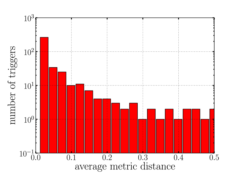
In Fig. 4 we show the distribution of metric distances (the minimum value for which the ellipsoids centred on the triggers overlap) for coincident triggers associated with simulated GW signals (see Sec IV.3). The number of coincidences falls off rapidly with increasing metric distances, whereas it would remain approximately constant for background coincident triggers generated by noise. However, it is the quieter triggers from farther GW sources (which are statistically more likely) that are recovered with the largest metric distances. Therefore larger coincidence ellipsoids can improve the overall sensitivity of a search.

Figure 4: Distribution of average parameter-space distance between coincident triggers associated with simulated GW signals in a month of representative S5 data, as recovered by the LIGO H1 and L1 detectors.

The result of the coincidence process is a list of all triggers that have SNR above threshold in two or more detectors and consistent parameters (masses and coalescence times) across detectors. When more than two detectors are operational, different combinations and higher-multiplicity coincidences are possible (e.g., three detectors yield triple coincidences and three types of double coincidences).

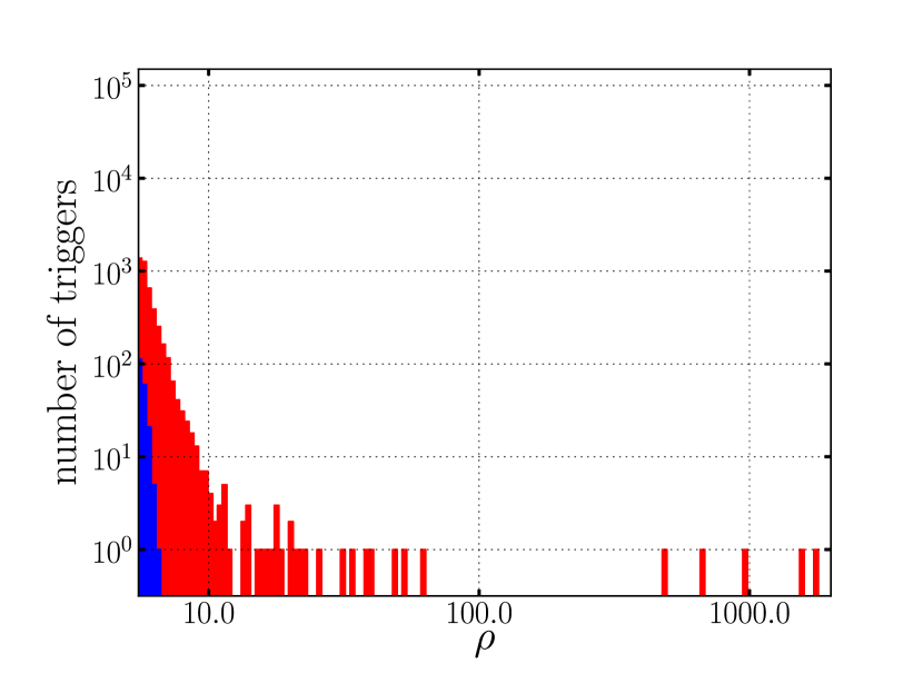
In Fig. 5 we show the distribution of coincident H1 triggers as a function of SNR in a month of simulated Gaussian noise (blue) and real S5 LIGO data (red). The largest single-detector SNRs for Gaussian noise are $\sim 7\mbox{--}8$, comparable (although somewhat larger) with early theoretical expectations Schutz (1989); Cutler et al. (1993). However, the distribution in real data is significantly worse, with SNRs of hundreds and even thousands. If we were to end our analysis here, a GW search in real data would be a hundred times less sensitive (in distance) than a search in Gaussian, stationary noise with the same PSD.

Figure 5: Distribution of single detector SNRs for H1 coincident triggers in a month of simulated Gaussian noise (blue) and representative S5 data (red). Coincidence was evaluated after time-shifting the SNR time series, so that only background coincidences caused by noise would be included. Comparison with Fig. 3 shows that the coincidence requirement reduces the high-SNR tail, but by no means eliminates it.

III IHOPE, part 2: mitigating the effects of non-Gaussian noise with signal-consistency tests, vetoes, and ranking statistics

To further reduce the tail of high-SNR triggers caused by the non-Gaussianity and nonstationarity of noise, the ihope pipeline includes a number of signal-consistency tests, which compare the properties of the data around the time of a trigger with those expected for a real GW signal. After removing duplicates, the coincident triggers in each $2048\text{\,}\mathrm{s}$ block are used to create a triggered template bank. Any template in a given detector that forms at least one coincident trigger in each $2048\text{\,}\mathrm{s}$ block will enter the triggered template bank for that detector and chunk. The new bank is again used to filter the data as described in Sec. II.3, but this time signal-consistency tests are also performed. These include the $\chi^{2}$ (Sec. III.1) and $r^{2}$ (Sec. III.2) tests. Coincident triggers are selected as described in Sec. II.4, and they are also tested for the consistency of relative signal amplitudes (Sec. III.3); at this stage, data-quality vetoes are applied (Sec. III.4) to sort triggers into categories according to the quality of data at their times.

The computational cost of the entire pipeline is reduced greatly by applying the expensive signal-consistency checks only in this second stage; the triggered template bank is, on average, a factor of $\sim 10$ smaller than the original template bank in the analysis described in Abbott et al. (2009c). However, the drawback is greater complexity of the analysis, and the fact that the coincident triggers found at the end of the two stages may not be identical.

III.1 The $\chi^{2}$ signal-consistency test

The basis of the $\chi^{2}$ test Allen (2005) is the consideration that although a detector glitch may generate triggers with the same SNR as a GW signal, the manner in which the SNR is accumulated over time and frequency is likely to be different. For example, a glitch that resembles a delta function corresponds to a burst of signal power concentrated in a small time-domain window, but smeared out across all frequencies. A CBC waveform, on the other hand, will accumulate SNR across the duration of the template, consistently with the chirp-like morphology of the waveform.

To test whether this is the case, the template is broken into $p$ orthogonal subtemplates with support in adjacent frequency intervals, in such a way that each subtemplate would generate the same SNR on average over Gaussian noise realizations. The actual SNR achieved by each subtemplate filtered against the data is compared to its expected value, and the squared residuals are summed. Thus, the $\chi^{2}$ test requires $p$ inverse Fourier transforms per template. For the low-mass CBC search, we found that setting $p=16$ provides a powerful discriminator without incurring an excessive computational cost Babak et al. (2005).

For a GW signal that matches the template waveform exactly, the sum of squared residuals follows the $\chi^{2}$ distribution with $2p-2$ degrees of freedom. For a glitch, or a signal that does not match the template, the expected value of the $\chi^{2}$-test is increased by a factor proportional to the total $\mathrm{SNR}^{2}$, with a proportionality constant that depends on the mismatch between the signal and the template. For signals, we may write the expected $\chi^{2}$ value as

$$\langle\chi^{2}\rangle=(2p-2)+\epsilon^{2}\rho^{2}\,,$$ (11)

where $\epsilon$ is a measure of signal–template mismatch. Even if CBC signals do not match template waveforms perfectly, due to template-bank discreteness, theoretical waveform inaccuracies Buonanno et al. (2009), spin effects Van Den Broeck et al. (2009), calibration uncertainties Abadie et al. (2010b), and so on, they will still yield significantly smaller $\chi^{2}$ than most glitches. It was found empirically that a good fraction of glitches are removed (with minimal effect on simulated signals) by imposing a SNR-dependent $\chi^{2}$ threshold of the form

$$\chi^{2}\leq\xi^{2}(p+\delta\rho^{2}),$$ (12)

with $\xi^{2}=10$ and $\delta=0.2$.

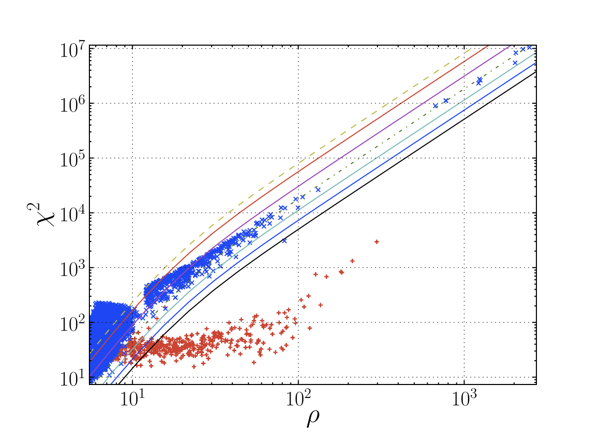
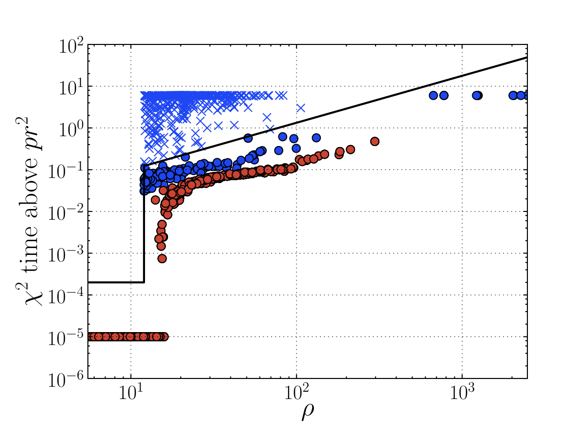
In Fig. 6 we show the distribution of $\chi^{2}$ as a function of SNR. A large number of triggers would have appeared in the upper left corner of the plot (large $\chi^{2}$ value relative to the measured SNR), but these have been removed by the cut. Even following the cut, a clear separation between noise background and simulated signals can easily be observed. This will be used later in formulating a detection statistic that combines the values of both $\rho$ and $\chi^{2}$.

Figure 6: The $\chi^{2}$ test plotted against SNR for triggers in a month of representative S5 data after the $\chi^{2}$ test has been applied, and the $r^{2}$ cut has been applied for triggers with $\rho<12$. The blue crosses mark time shifted background triggers, the red pluses mark simulated-GW triggers. The solid, colored lines on the plots indicate lines of constant effective SNR (top panel) and new SNR (bottom panel), which are described in section III.5. Larger values of effective/new SNR are at the bottom and right end of the plots. The clearly visible notch in the H1 and L1 plots is caused by the discontinuity in the $r^{2}$ cut at an SNR of 12 (Section III.2). Here background triggers are represented by blue crosses and injections by red pluses.

III.2 The $r^{2}$ signal-consistency test

We can also test the consistency of the data with a postulated signal by examining the time series of SNRs and $\chi^{2}$s. For a true GW signal, this would show a single sharp peak at the time of the signal, with the width of the falloff determined by the autocorrelation function of the template Hanna (2008); Harry and Fairhurst (2011). Thus, counting the number of time samples around a trigger for which the SNR is above a set threshold provides a useful consistency test Shawhan and Ochsner (2004). Examining the behavior of the $\chi^{2}$ time series provides a more powerful diagnostic Rodríguez (2007). To wit, the $r^{2}$ test sets an upper threshold on the amount of time $\Delta T$ (in a window $T$ prior to the trigger) for which

$$\chi^{2}\geq p\,r^{2},$$ (13)

where $p$ is the number of subtemplates used to compute the $\chi^{2}$. We found empirically that setting $T=6\text{\,}\mathrm{s}$ and $r^{2}=15$ produces a powerful test Rodríguez (2007). Figure 7 shows the characteristic shape of the $\chi^{2}$ time series for CBC signals: close to zero when the template is aligned with the signal, then increasing as the two are offset in time, before falling off again with larger time offsets.

Figure 7: Value of SNR and $\chi^{2}$ as a function of time, for a simulated CBC signal with SNR=300 in a stretch of S5 data from the H1 detector. The SNR shows a characteristic rise and fall around the signal. The $\chi^{2}$ value is small at the time of the signal, but increases steeply to either side as the template waveform is offset from the signal in the data.

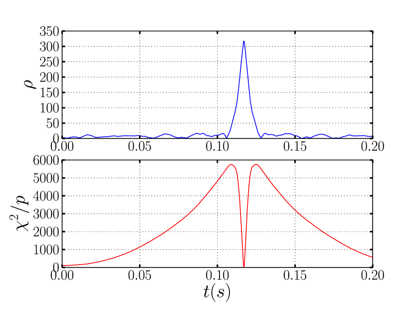
An effective $\Delta T$ threshold must be a function of SNR; the $\Delta T$ commonly used for ihope searches is

$$\Delta T<\left\{\begin{array}[]{ll}\displaystyle 2\times 10^{-4}\,\mathrm{s}&\text{for $\rho<12$},\\ \displaystyle\rho^{9/8}\times 7.5\times 10^{-3}\,\mathrm{s}&\text{for $\rho\geq 12$}.\end{array}\right.$$ (14)

The threshold for $\rho<12$ eliminates triggers for which any sample is above the threshold from equation (13).

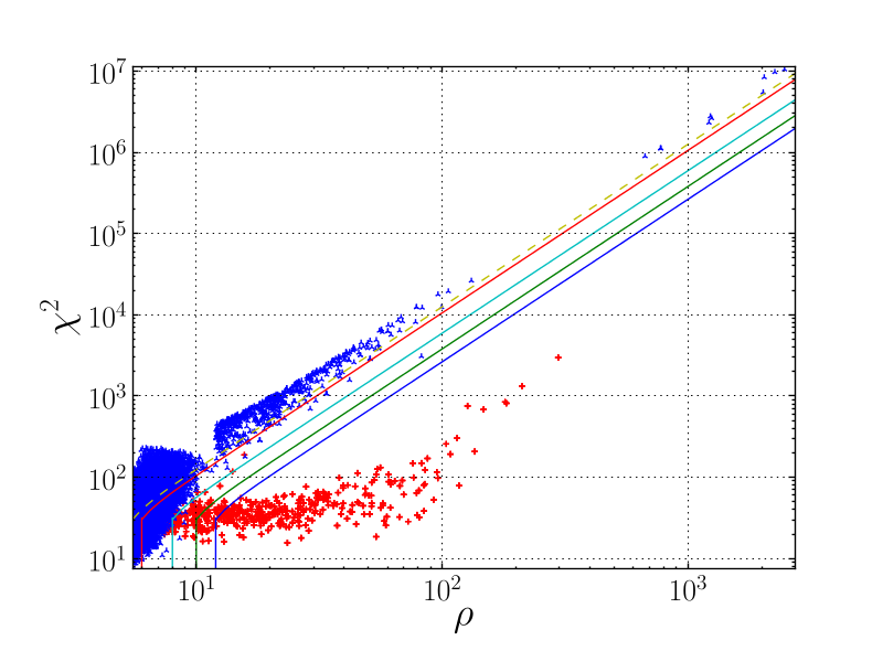
In Fig. 8 we show the effect of such an SNR test. For $\rho<12$, the value of $\Delta T$ is smaller than the sample rate, therefore triggers are discarded if there are any time samples in the $6\text{\,}\mathrm{s}$ prior to the trigger for which Eq. (13) is satisfied. (Since the $6\text{\,}\mathrm{s}$ window includes the trigger, for some SNRs this imposes a more stringent requirement than the $\chi^{2}$ test (12), explaining the notch at $\rho<12$ and relatively large $\chi^{2}$ values in Fig. 6.) For $\rho\geq 12$, the threshold is SNR dependent. The $r^{2}$ test is powerful at removing a large number of high-SNR background triggers (the blue crosses), without affecting the triggers produced by simulated GW signals (the red circles). The cut is chosen to be conservative to allow for any imperfect matching between CBC signals and template waveforms.

Figure 8: The $\chi^{2}$ time above $pr^{2}$ as a function of SNR, for all second-stage H1 triggers in a month of representative S5 data. The $r^{2}$ test has already been applied on triggers with $\rho<12$, and only those surviving the cut are shown. The blue crosses mark all background triggers (with $\rho>12$) that fail the cut; blue circles indicate background triggers that pass it. Red circles mark simulated-GW triggers, none of which are cut.

III.3 Amplitude-consistency tests

The two LIGO Hanford detectors H1 and H2 share the same vacuum tubes, and therefore expose the same sensitive axes to any incoming GW. Thus, the ratio of the H1 and H2 SNRs for true GW signals should equal the ratio of detector sensitivities. We can formulate a formal test of H1–H2 amplitude consistency in terms of a GW source’s effective distance $D_{\mathrm{eff},A}$—the distance at which an optimally located and oriented source would give the SNR observed with detector $A$. Namely, we require that

$$\kappa=2\frac{\left|D_{\mathrm{eff,H1}}-D_{\mathrm{eff,H2}}\right|}{D_{\mathrm{eff,H1}}+D_{\mathrm{eff,H2}}}\leq\kappa^{*};$$ (15)

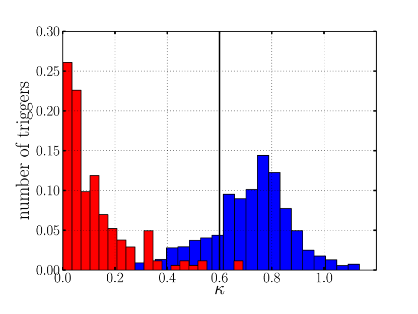
setting a threshold $\kappa^{*}$ provides discrimination against noise triggers while allowing for some measurement uncertainty. In Fig. 9 we show the distribution of $\kappa$ for simulated-GW triggers and background triggers in a month of representative S5 data. We found empirically that setting $\kappa^{*}=0.6$ produces a powerful test.

Figure 9: Distribution of $\kappa$ [Eq. (15)], the fractional difference in the effective distances measured by H1 and H2 for coincident triggers in those detectors in a month of representative S5 data. Background triggers (blue) tend to have larger $\kappa$ than simulated-GW triggers (red).

An amplitude-consistency test can be defined also for triggers that are seen in only one of H1 and H2. We do this by removing any triggers from H1 which are loud enough that we would have expected to observe a trigger in H2 (and vice-versa). We proceed by calculating $\sigma_{A}$, the distance at which an optimally located and oriented source yields an SNR of 1 in detector $A$, and noting that $D_{\mathrm{eff},A}=\sigma_{A}/\rho_{A}$. Then, by rearranging (15), we are led to require that a trigger that is seen only in H1 satisfy

$$\rho_{\mathrm{H1}}<\frac{\sigma_{\mathrm{H1}}}{\sigma_{\mathrm{H2}}}\left(\frac{2+\kappa^{*}}{2-\kappa^{*}}\right)\rho^{*}_{\mathrm{H2}},$$ (16)

where $\rho^{*}_{\mathrm{H2}}$ is the SNR threshold used for H2. The effective distance cut removes essentially all H2 triggers for which there is no H1 coincidence: since H2 typically had around half the distance sensitivity of H1, a value of $\kappa^{*}=0.6$ imposes $\rho_{\mathrm{H2}}<\rho_{\mathrm{H1}}^{*}$.

Neither test was used between any other pair of detectors because, in principle, any ratio of effective distances is possible for a real signal seen in two nonaligned detectors. However, large values of $\kappa$ are rather unlikely, especially for the Hanford and Livingston LIGO detectors, which are almost aligned. Therefore amplitude-consistency tests should still be applicable.

III.4 Data-quality vetoes

Environmental factors can cause periods of elevated detector glitch rate. In the very worst (but very rare) cases, this makes the data essentially unusable. More commonly, if these glitchy periods were analyzed together with periods of relatively clean data, they could produce a large number of high-SNR triggers, and possibly mask GW candidates in clean data. It is therefore necessary to remove or separate the glitchy periods.

This is accomplished using data quality (DQ) flags Slutsky et al. (2010); Christensen (2010) (for the LIGO Scientific Collaboration and the Virgo Collaboration); Aasi et al. (2012). All detectors are equipped with environmental and instrumental monitors; their output is recorded in the detector’s auxiliary channels. Periods of heightened activity in these channels (e.g., as caused by elevated seismic noise MacLeod et al. (2012)) are automatically marked with DQ flags Ito . DQ flags can also be added manually if the detector operators observe poor instrumental behavior.

If a DQ flag is found to be strongly correlated with CBC triggers, and if the flag is safe (i.e., not triggered by real GWs), then it can be used a DQ veto. Veto safety is assessed by comparing the fraction of hardware GW injections that are vetoed with the total fraction of data that is vetoed. During the S6 and VSR2-3 runs, a simplified form of ihope was run daily on the preceding 24 hours of data from each detector individually, specifically looking for non-Gaussian features that could be correlated with instrumental or environmental effects Pekowsky (2012); MacLeod et al. (2012). The results of these daily runs were used to help identify common glitch mechanisms and to mitigate the effects of non-Gaussian noise by suggesting data quality vetoes.

Vetoes are assigned to categories based on the severity of instrumental problems and on how well the couplings between the GW and auxiliary channels are understood Slutsky et al. (2010); Christensen (2010) (for the LIGO Scientific Collaboration and the Virgo Collaboration); Aasi et al. (2012). Correspondingly, CBC searches assign data to four DQ categories:

Category 1

Seriously compromised or missing data. The data are entirely unusable, to the extent that they would corrupt noise PSD estimates. These times are excluded from the analysis, as if the detector was not in science mode (introduced in Sec. II.1).

Category 2

Instrumental problems with known couplings to the GW channel. Although the data are compromised, these times can still be used for PSD estimation. Data flagged as category-2 are analyzed in the pipeline, but any triggers occurring during these times are discarded. This reduces the fragmentation of science segments, maximizing the amount of data that can be analyzed.

Category 3

Likely instrumental problems, casting doubt on triggers found during these times. Data flagged as category-3 are analyzed and triggers are processed. However, the excess noise in such times may obscure signals in clean data. Consequently, the analysis is also performed excluding time flagged as category-3, allowing weaker signals in clean data to be extracted. These data are excluded from the estimation of upper limits on GW-event rates.

Good data

Data without any active environmental or instrumental source of noise transients. These data are analyzed in full.

Poor quality data are effectively removed from the analysis, reducing the total amount of analyzed time. For instance, in the third month of the S5 analysis reported in Ref. Abbott et al. (2009c), removing category-1 times left $1.2\times 10^{6}\text{\,}\mathrm{s}$ of data when at least two detectors were operational; removing category-2 and -3 times left $1.0\times 10^{6}\text{\,}\mathrm{s}$, although the majority of lost time was category-3, and was therefore analyzed for loud signals.

III.5 Ranking statistics

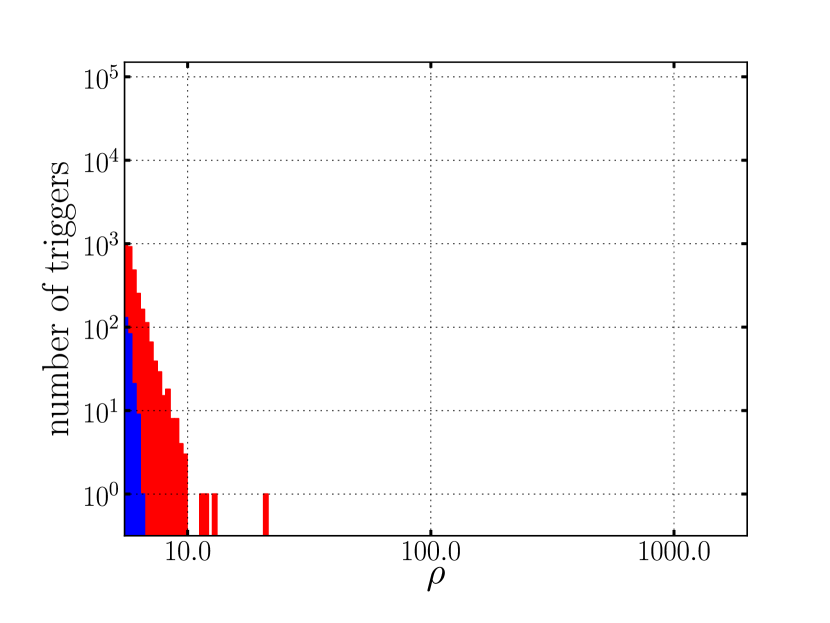
The application of signal-consistency and amplitude-consistency tests, as well as data-quality vetoes, is very effective in reducing the non-Gaussian tail of high-SNR triggers. In Fig. 10 we show the distribution of H1 triggers that are coincident with triggers in the L1 detector (in time shifts) and that pass all cuts. For consistency, identical cuts have been applied to the simulated, Gaussian data, including vetoing times of poor data quality in the real data. The majority of these have minimal impact, although the data quality vetoes will remove a (random) fraction of the triggers arising in the simulated data analysis.

Remarkably, in the real data, almost no triggers are left that have $\mathrm{SNR}>10$. Nevertheless, a small number of coincident noise triggers with large SNR remain. These triggers have passed all cuts, but they generally have significantly worse $\chi^{2}$ values than expected for true signals, as we showed in Fig. 6.

Figure 10: Distribution of single detector SNRs for H1 triggers found in coincidence with L1 triggers (in time shifts) in a month of simulated Gaussian noise (blue) and representative S5 data (red). These triggers have survived $\chi^{2}$, $r^{2}$, and H1–H2 amplitude-consistency tests, as well as DQ vetoes.

It is therefore useful to rank triggers using a combination of SNR and $\chi^{2}$, by introducing a re-weighted SNR. Over the course of the LIGO-Virgo analyses, several distinct re-weighted SNRs have been used. For the LIGO S5 run and Virgo’s first science run (VSR1), we adopted the effective SNR $\rho_{\mathrm{eff}}$, defined as Abbott et al. (2009b)

$$\rho^{2}_{\rm eff}=\frac{\rho^{2}}{\sqrt{\left(\frac{\chi^{2}}{n_{\mathrm{dof}}}\right)\left(1+\frac{\rho^{2}}{250}\right)}}\,,$$ (17)

where $n_{\mathrm{dof}}=2p-2$ is the number of $\chi^{2}$ degrees of freedom, and the factor $250$ was tuned empirically to provide separation between background triggers and simulated GW signals. The normalization of $\rho_{\mathrm{eff}}$ ensures that a “quiet” signal with $\rho\simeq 8$ and $\chi^{2}$ $\simeq n_{\mathrm{dof}}$ will have $\rho_{\mathrm{eff}}\simeq\rho$.

Figure 6 shows contours of constant $\rho_{\mathrm{eff}}$ in the $\rho$–$\chi^{2}$ plane. While $\rho_{\mathrm{eff}}$ successfully separates background triggers from simulated-GW triggers, it can artificially elevate the SNR of triggers with unusually small $\chi^{2}$. As discussed in Ref. Abadie et al. (2011), these can sometimes become the most significant triggers in a search. Thus, a different statistic was adopted for the LIGO S6 run and Virgo’s second and third science runs (VSR23). This new SNR $\rho_{\mathrm{new}}$ Abadie et al. (2012a) was defined as

$$\rho_{\mathrm{new}}=\left\{\begin{array}[]{cl}\rho&\text{for $\chi^{2}\leq n_{\mathrm{dof}}$},\\ \rho\left[\frac{1}{2}\left(1+\left(\frac{\chi^{2}}{n_{\mathrm{dof}}}\right)^{\!3}\right)\right]^{-1/6}&\text{for $\chi^{2}>n_{\mathrm{dof}}$}.\end{array}\right.$$ (18)

Figure 6 also shows contours of constant $\rho_{\mathrm{new}}$ in the $\rho$–$\chi^{2}$ plane. The new SNR was found to provide even better background–signal separation, especially for low-mass nonspinning inspirals Abadie et al. (2012a), and it has the desirable feature that $\rho_{\mathrm{new}}$ does not take larger values than $\rho$ when the $\chi^{2}$ is less than the expected value. Other ways of defining a detection statistic as a function of $\rho$ and $\chi^{2}$ can be defined and optimized for analyses covering different regions of parameter space and different data sets.

For coincident triggers, the re-weighted SNRs measured in the coincident detectors are added in quadrature to give a combined, re-weighted SNR, which is used to rank the triggers and evaluate their statistical significance. Using this ranking statistic, we find that the distribution of background triggers in real data is remarkably close to their distribution in simulated Gaussian noise. Thus, our consistency tests and DQ vetoes have successfully eliminated the vast majority of high SNR triggers due to non-Gaussian noise from the search. While this comes at the inevitable cost of missing potential detections at times of poor data quality, it significantly improves the detection capability of a search.

Figure 11: Distribution of single detector new SNR, $\rho_{\mathrm{new}}$, for H1 triggers found in coincidence with L1 triggers (in time shifts) in a month of simulated Gaussian noise (blue) and representative S5 data (red). The tail of high SNR triggers due to non-Gaussian noise has been virtually eliminated—a remarkable achievement given that the first stage of the pipeline generated single-detector triggers with $\mathrm{SNR}>1,000$.

IV Interpretation of the Results

At the end of the data processing described above, the ihope pipeline produces a set of coincident triggers ranked by their combined re-weighted SNR; these triggers have passed the various signal-consistency and data-quality tests outlined above. While at this stage the majority of loud background triggers identified in real data have been eliminated or downweighted, the distribution of triggers is still different from the case of Gaussian noise, and it depends on the quality of the detector data and the signal parameter space being searched over. Therefore it is not possible to derive an analytical mapping from combined re-weighted SNR to event significance, as characterized by the FAR. Instead, the FAR is evaluated empirically by performing numerous time-shift analyses, in which artificial time shifts are introduced between the data from different detectors. (These are discussed in Sec. IV.1.) Furthermore, the rate of triggers as a function of combined re-weighted SNR varies over parameter space; to improve the FAR accuracy, we divide triggers into groups with similar combined re-weighted SNR distributions (see Sec. IV.2). The sensitivity of a search is evaluated by measuring the rate of recovery of a large number of simulated signals, with parameters drawn from astrophysically motivated distributions (see Sec. IV.3). The sensitivity is then used to estimate the CBC event rates or upper limits as a function of signal parameters (see Sec. IV.4).

IV.1 Background event rate from time shifts

The rate of coincident triggers as a function of combined re-weighted SNR is estimated by performing numerous time-shift analyses: in each we artificially introduce different relative time shifts in the data from each detector Amaldi et al. (1989). The time shifts that are introduced must be large enough such that each time-shift analysis is statistically independent.

To perform the time-shift analysis in practice, we simply shift the triggers generated at the first matched-filtering stage of the analysis (II.3), and repeat all subsequent stages from multi-detector coincidence (II.4) onwards. Shifts are performed on a ring: for each time-coincidence period (i.e., data segment where a certain set of detectors is operational), triggers that are shifted past the end are re-inserted at the beginning. Since the time-coincidence periods are determined before applying Category-2 and -3 DQ flags, there is some variation in analyzed time among time-shift analyses. To ensure statistical independence, time shifts are performed in multiples of $5\text{\,}\mathrm{s}$; this ensures that they are significantly larger than the light travel time between the detectors, the autocorrelation time of the templates, and the duration of most non-transient glitches seen in the data. Therefore, any coincidences seen in the time shifts cannot be due to a single GW source, and are most likely due to noise-background triggers. It is possible, however, for a GW-induced trigger in one detector to arise in time-shift coincidence with noise in another detector. Indeed, this issue arose in Ref. Abadie et al. (2012a), where a “blind injection” was added to the data to test the analysis procedure.

The H1 and H2 detectors share the Hanford beam tubes and are affected by the same environmental disturbances; furthermore, noise transients in the two detectors have been observed to be correlated. Thus, time-shift analysis is ineffective at estimating the coincident background between these co-located detectors, and it is not used. Coincident triggers from H1 and H2 when no other detectors are operational are excluded from the analysis. When detectors at additional sites are operational, we do perform time shifts, keeping H1 and H2 “in time” but shifting both relative to the other detectors.

Our normal practice is to begin by performing 100 time-shift analyses to provide an estimate of the noise background. If any coincident in-time triggers are still more significant (i.e., have larger combined re-weighted SNR) than all the time-shifted triggers, additional time shifts are performed to provide an estimate of the FAR. A very significant candidate would have a very low FAR, and an accurate determination of its FAR requires a large number of time slides: in Ref. Abadie et al. (2012a) over a million were performed. However, there is a limit to the number of statistically independent time shifts that are possible to perform, as explored in Was et al. (2010). Additionally, as the number of time shifts grows, the computational savings of our two-stage search are diminished, because a greater fraction of the templates survive to the second filtering stage where the computationally costly signal-consistency tests are performed (see Sec. III.1). We are currently investigating whether it is computationally feasible to run ihope as a single-stage pipeline and compute $\chi^{2}$ and $r^{2}$ for every trigger.

IV.2 Calculation of false-alarm rates

The FAR for a coincident trigger is given by the rate at which background triggers with the same or greater SNR occur due to detector noise. This rate is computed from the time-shift analyses; for a fixed combined re-weighted SNR, it varies across the template mass space, and it depends on which detectors were operational and how glitchy they were. To accurately account for this, coincident triggers are split into categories, and FARs are calculated within each, relative to a background of comparable triggers. The triggers from each category are then re-combined into a single list and ranked by their FARs.

Figure 12: Fraction of time-shift coincident triggers between H1 and L1 in a month of representative S5 data that have combined new SNR greater than or equal to the x-axis value, for three chirp-mass bins. The distribution from a month of Gaussian noise is also shown for comparison. The tails of the distributions become more shallow for larger chirp masses $\mathcal{M}$, so triggers with higher $\mathcal{M}$ are more likely to have higher SNRs.

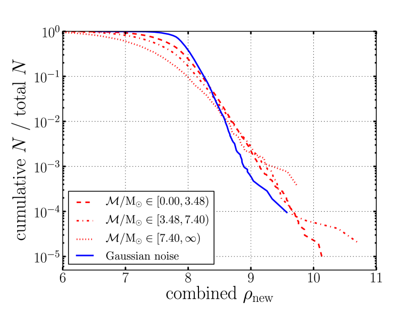
Typically, signal-consistency tests are more powerful for longer-duration templates than for shorter ones, so the non-Gaussian background is suppressed better for low-mass templates, while high-mass templates are more likely to result in triggers with larger combined re-weighted SNRs. In recent searches, triggers have been separated into three bins in chirp mass $\mathcal{M}$ Brown (2004): $\mathcal{M}\leq 3.48\,M_{\odot}$, $3.48\,M_{\odot}<\mathcal{M}\leq 7.4\,M_{\odot}$, and $\mathcal{M}>7.4\,M_{\odot}$. Figure 12 shows the distribution of coincident triggers between H1 and L1 as a function of combined $\rho_{\mathrm{new}}$ for the triggers in each of these mass bins. As expected, the high-$\mathcal{M}$ bin has a greater fraction of high-SNR triggers.

The combined re-weighted SNR is calculated as the quadrature sum of the SNRs in the individual detectors. However, different detectors can have different rates of non-stationary transients as well as different sensitivities, so the combined SNR is not necessarily the best measure of the significance of a trigger. Additionally, background triggers found in three-detector coincidence will have a different distribution of combined re-weighted SNRs than two-detector coincident triggers Abbott et al. (2009b). Therefore, we separate coincident triggers by their type, which is determined by the coincidence itself (e.g., H1H2, or H1H2L1) and by the availability of data from each detector, known as “coincident time.” Thus, the trigger types would include H1L1 coincidences in H1L1 double-coincident time; H1L1, H1V1, L1V1, and H1L1V1 coincidences in H1L1V1 triple-coincident time; and so on. When H1 and H2 are both operational, we have fewer coincidence types than might be expected as H1H2 triggers are excluded due to our inability to estimate their background distribution, and the effective distance cut removes H2L1 or H2V1 coincidences. The product of mass bins and trigger types yields all the trigger categories.

For simplicity, we treat times when different networks of detectors were operational as entirely separate experiments; this is straightforward to do, as there is no overlap in time between them. Furthermore, the data from a long science run is typically broken down into a number of distinct stretches, often based upon varying detector sensitivity or glitchiness, and each is handled independently.

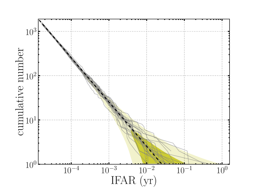
For each category of coincident triggers within an experiment, an additional clustering stage is applied. If there is another coincident trigger with a larger combined re-weighted SNR within $10\text{\,}\mathrm{s}$ of a given trigger’s end time, the trigger is removed. We then compute the FAR as a function of combined re-weighted SNR as the rate (number over the total coincident, time-shifted search time) of time-shift coincidences observed with higher combined re-weighted SNR within each category. These results must then be combined to estimate the overall significance of triggers: we calculate a combined FAR across categories by ranking all triggers by their FAR, counting the number of more significant time-shift triggers, and dividing by the total time-shift time. The resulting combined FAR is essentially the same as the uncombined FAR, multiplied by the number of categories that were combined. We often quote the inverse FAR (IFAR) as the ranking statistic, so that more significant triggers correspond to larger values. A loud GW may produce triggers in more than one mass bin, and consequently more than one candidate trigger might be due to a single event. This is resolved by reporting only the coincident trigger with the largest IFAR associated with a given event. Figure 13 shows the expected mean (the dashed line) and variation (the shaded areas) of the cumulative number of triggers as a function of IFAR for the analysis of three-detector H1H2L1 time in a representative month of S5 data. The variations among time shifts (the thin lines) match the expected distribution. The duration of the time-shift analysis is $\sim 10^{8}\text{\,}\mathrm{s}$, but taking into account the six categories of triggers (three mass bins and two coincidence types), this yields a minimum FAR of $\sim 1\text{\,}\invyear$.

Clearly a FAR of $\sim 1\text{\,}\invyear$ is insufficient to confidently identify GW events. The challenge of extending background estimation to the level where a loud trigger can become a detection candidate was met in the S6–VSR2/3 search Abadie et al. (2012a); Dent et al. . Remarkably, even for FARs of one in tens of thousands of years, no tail of triggers with large combined re-weighted SNRs was observed. Evidently, the cuts, tests, and thresholds discussed in Section III are effective at eliminating any evidence of a non-Gaussian background, at least for low chirp masses.

Figure 13: Cumulative histogram of triggers vs. IFAR for all time-shift triggers in H1H2L1 triple-coincident time from a representative month of S5 data. The black dashed line marks the expected cumulative number, while the shaded regions mark its 1- and 2-$\sigma$ variation. The thin grey lines show the cumulative number for 20 of the time shifts, providing an additional indication of the expected deviation from the mean.

In calculating the FAR, we treat all trigger categories identically, so we implicitly assign the same weight to each. However, this is not appropriate when the detectors have significantly different sensitivities, since a GW is more likely to be observed in the most sensitive detectors. In the search of LIGO S5 and Virgo VSR1 data Abadie et al. (2010a), this approach was refined by weighting the categories on the basis of the search sensitivity for each trigger type. However, if there were an accurate astrophysical model of CBC merger rates for different binary masses, the weighting could easily be extended to the mass bins.

IV.3 Evaluating search sensitivity

The sensitivity of a search is measured by adding simulated GW signals to the data and verifying their recovery by the pipeline, which also helps tune the pipeline’s performance against expected sources. The simulated signals can be added as hardware injections Brown (for the LIGO Scientific Collaboration); Abadie et al. (2012a), by actuating the end mirrors of the interferometers to reproduce the response of the interferometer to GWs; or as software injections, by modifying the data after it has been read into the pipeline. Hardware injections provide a better end-to-end test of the analysis, but only a limited number can be performed, since the data containing hardware injections cannot be used to search for real GW signals. Consequently, large-scale injection campaigns are performed in software.

Software injections are performed into all operational detectors coherently (i.e., with relative time delays, phases and amplitudes appropriate for the relative location and orientation of the source and the detectors). Simulated GW sources are generally placed uniformly over the celestial sphere, with uniformly distributed orientations. The mass and spin parameters are generally chosen to uniformly cover the search parameter space, since they are not well constrained by astrophysical observations, particularly so for binaries containing black holes Mandel and O’Shaughnessy (2010). Although sources are expected to be roughly uniform in volume, we do not follow that distribution for simulations, but instead attempt to place a greater fraction of injections at distances where they would be marginally detectable by the pipeline. The techniques used to reduce the dimensionality of parameter space, such as analytically maximizing the detection statistic, cannot be applied to the injections, which must cover the entire space. This necessitates large simulation campaigns.

The ihope pipeline is run on the data containing simulated signals using the same configuration as for the rest of the search. Injected signals are considered to be found if there is a coincident trigger within $1\text{\,}\mathrm{s}$ of their injection time. The loudest coincident trigger within the $1\text{\,}\mathrm{s}$ window is associated with the injection, and it may be louder than any trigger in the time-shift analyses (i.e., it may have a FAR of zero). Using a $1\text{\,}\mathrm{s}$ time window to associate triggers and injections and no requirement on mass consistency may lead to some of these being found spuriously, in coincidence with background triggers. However, this effect has negligible consequences on the estimated search sensitivity near the combined re-weighted SNR of the most significant trigger.

Figure 14: Found and missed injections in one month of S5 data plotted at their chirp mass $\mathcal{M}$ and decisive distance (see main text for definition). Red crosses are missed injections; colored circles are injections found with non-zero combined FAR, which can be read off the colormap on the right; black stars are injections found with FAR = 0 (i.e., associated with triggers louder than any in the background from 100 time shifts). Nearby injections that are missed or found with high FARs are followed up to check for problems in the pipeline, and to improve data quality.

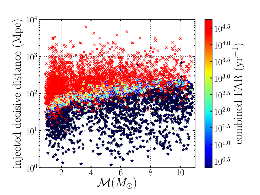
Figure 14 shows the results of a large number of software injections performed in one month of S5 data. For each injection, we indicate whether the signal was missed (red crosses) or found (circles, and stars for FAR = 0). The recovery of simulated signals can be compared with the theoretically expected sensitivity of the search, taking into account variations over parameter space: the expected SNR of a signal is proportional to $\mathcal{M}^{5/6}$ (for low-mass binaries), inversely proportional to effective distance (see Sec. III.3), and a function of the detectors’ noise PSD. An insightful way to display injections, used in Fig. 14, is to show their chirp mass $\mathcal{M}$ and decisive distance—the second largest effective distance for the detectors that were operating at the time of the injection (in a coincidence search, it is the second most sensitive detector that limits the overall sensitivity). Indeed, our empirical results are in good agreement with the stated sensitivity of the detectors Abadie et al. (2010c, 2012b). A small number of signals are missed at low distances: these are typically found to lie close to loud non-Gaussian glitches in the detector data.

IV.4 Bounding the binary coalescence rate

The results of a search can be used to estimate (if positive detections are reported) or bound the rate of binary coalescences. An upper limit on the merger rate is calculated by evaluating the sensitivity of the search at the loudest observed trigger Brady et al. (2004); Brady and Fairhurst (2008); Biswas et al. (2009); Keppel (2009). Heuristically, the 90% rate upper limit corresponds to a few (order 2–3) signals occurring over the search time within a small enough distance to generate a trigger with IFAR larger than the loudest observed trigger.

More specifically, we assume that CBC events occur randomly and independently, and that the event rate is proportional to the star-formation rate, which is itself assumed proportional to blue-light galaxy luminosity Phinney (1991). For searches sensitive out to tens or hundreds of megaparsecs, it is reasonable to approximate the blue-light luminosity as uniform in volume, and quote rates per unit volume and time Abadie et al. (2010d). We follow Biswas et al. (2009); Abbott et al. (2009b) and infer the probability density for the merger rate $R$, given that in an observation time $T$ no other trigger was seen with IFAR larger than its loudest-event value, $\alpha_{m}$:

$$p(R|\alpha_{m},T)\propto p(R)\,e^{-RV(\alpha_{m})T}\left(1+\Lambda(\alpha_{m})R\,T\,V(\alpha_{m})\right);$$ (19)

here $p(R)$ is the prior probability density for $R$, usually taken as the result of previous searches or as a uniform distribution for the first search of a kind; $V(\alpha)$ is the volume of space in which the search could have seen a signal with $\mathrm{IFAR}\geq\alpha$; and the quantity $\Lambda$ is the relative probability that the loudest trigger was due to a GWs rather than noise,

$$\Lambda=\frac{\lvert V^{\prime}(\alpha_{m})\rvert}{V(\alpha_{m})}\frac{P_{B}(\alpha_{m})}{P^{\prime}_{B}(\alpha_{m})},\quad\text{with}\quad P_{B}(\alpha)=e^{-T/\alpha},$$ (20)

with the prime denoting differentiation with respect to $\alpha$. For a chosen confidence level $\gamma$ (typically 0.9 = 90%), the upper limit $R_{\ast}$ on the rate is then given by

$$\gamma=\int^{R_{\ast}}_{0}p(R|\alpha_{m},T)\,dR.$$ (21)

Figure 15: Search efficiency for binary neutron star (BNS) injections in a month of representative S5 data (blue) and in Gaussian noise (red), for a false-alarm rate equal to the FAR of the loudest foreground trigger in each analysis.

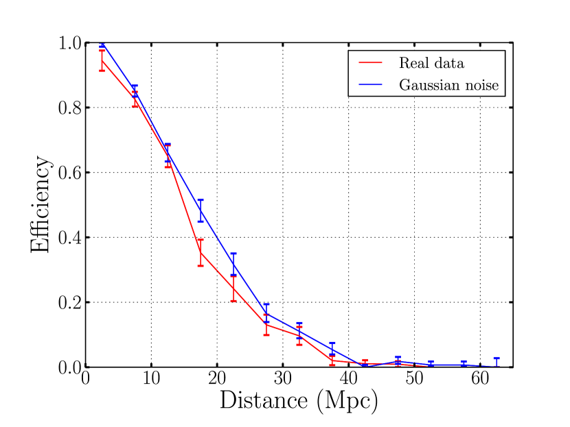
It is clear from Eq. (19) that the decay of $p(R|\alpha_{m},T)$ and the resulting $R_{\ast}$ depend critically on the sensitive volume $V(\alpha_{m})$. In previous sections we have shown how ihope is highly effective at filtering out triggers due to non-Gaussian noise, thus improving sensitivity, and in the context of computing upper limits, we can quantify the residual effects of non-Gaussian features on $V(\alpha_{m})$. In Fig. 15 we show the search efficiency for BNS signals, i.e. the fraction of BNS injections found with IFAR above a fiducial value, here set to the IFAR of the loudest in-time noise trigger as a function of distance, for one month of S5 data and for a month of Gaussian noise with the same PSDs. Despite the significant non-Gaussianity of real data, the distance at which efficiency is 50% is reduced by $\sim 10$% and the sensitive search volume by $\sim 30$%, compared to Gaussian-noise expectations.

V Discussion and future developments

In this paper we have given a detailed description of the ihope software pipeline, developed to search for GWs from CBC events in LIGO and Virgo data, and we have provided several examples of its performance on a sample stretch of data from the LIGO S5 run. The pipeline is based on a matched-filtering engine augmented by a substantial number of additional modules that implement coincidence, signal-consistency tests, data-quality cuts, tunable ranking statistics, background estimation by time shifts, and sensitivity evaluation by injections. Indeed, with the ihope pipeline we can run analyses that go all the way from detector strain data to event significance and upper limits on CBC rates.

The pipeline was developed over a number of years, from the early versions used in LIGO’s S2 BNS search to its mature incarnation used in the analysis of S6 and VSR3 data. One of the major successes of the ihope pipeline was the mitigation of spurious triggers from non-Gaussian noise transients, to such an extent that the overall volume sensitivity is reduced by less than 20% compared to what would be possible if noise was Gaussian. Nevertheless, there are still significant improvements that can and must be made to CBC searches if we are to meet the challenges posed by analyzing the data of advanced detectors. In the following paragraphs, we briefly discuss some of these improvements and challenges.

Coherent analysis.

As discussed above, the ihope pipeline comes close to the sensitivity that would be achieved if noise was Gaussian, with the same PSD. Therefore, while some improvement could be obtained by implementing more sophisticated signal-consistency tests and data-quality cuts, it will not be significant. If three or more detectors are active, sensitivity would be improved in a coherent Finn and Chernoff (1993); Pai et al. (2001); Harry and Fairhurst (2011) (rather than coincident) analysis that filters the data from all operating detectors simultaneously, requiring consistency between the times of arrival and relative amplitudes of GW signals, as observed in each data stream. Such a search is challenging to implement because the data from the detectors must be combined differently for each sky position, significantly increasing computational cost.

Coherent searches have already been run for unmodeled burst-like transients Abadie et al. (2010e), and for CBC signals in coincidence with gamma-ray-burst observations Briggs et al. (2012), but a full all-sky, all-time pipeline like ihope would require significantly more computation. A promising compromise may be a hierarchical search consisting of a first coincidence stage followed by the coherent analysis of candidates, although the estimation of background trigger rates would prove challenging as time shifts in a coherent analysis cannot be performed using only the recorded single detector triggers but require the full SNR time series.

Background estimation.

The first positive GW detection requires that we assign a very low false-alarm probability to a candidate trigger Abadie et al. (2012a). In the ihope pipeline, this would necessitate a large number of time shifts, thus negating the computational savings of splitting matched filtering between two stages, or a different method of background estimation Dent et al. ; Cannon et al. . Whichever the solution, it will need to be automated to identify signal candidates rapidly for possible astronomical follow up.

Event-rate estimation.

After the first detections, we will begin to quote event-rate estimates rather than upper limits. The loudest-event method can be used for this Biswas et al. (2009), provided that the data are broken up so that much less than one gravitational wave signal is expected in each analyzed stretch. There are however other approaches Messenger and Veitch that should be considered for implementation.

Template length.

The sensitive band of advanced detectors will extend to lower frequencies ($\sim 10\text{\,}\mathrm{Hz}$) than their first-generation counterparts, greatly increasing the length and number of templates required in a matched-filtering search. Increasing computational resources may not be sufficient, so we are investigating alternative approaches to filtering Marion et al. (2004); Cannon et al. (2010, 2011a, 2011b, 2012) and possibly the use of graphical processing units (GPUs).

Latency.

The latency of CBC searches (i.e., the “wall-clock” time necessary for search results to become available) has decreased over the course of successive science runs, but further progress is needed to perform prompt follow-up observations of GW candidate with conventional (electromagnetic) telescopes Abadie et al. (2012); Metzger and Berger (2012). The target should be posting candidate triggers within minutes to hours of data taking, which was in fact achieved in the S6–VSR3 analysis with the MBTA pipeline Marion et al. (2004).

Template accuracy.

While the templates currently used in ihope are very accurate approximations to BNS signals, they could still be improved for the purpose of neutron star–black hole (NSBH) and binary black hole (BBH) searches Buonanno et al. (2009). It is straightforward to extend ihope to include the effects of spin on the progress of inspiral (i.e., its phasing), but it is harder to include the orbital precession caused by spins and the resulting waveform modulations. The first extension would already improve sensitivity to BBH signals Ajith et al. (2011); Santamaria et al. (2010), but precessional effects are expected to be more significant for NSBH systems Pan et al. (2004); Ajith (2011).

Parameter estimation.

Last, while ihope effectively searches the entire template parameter space to identify candidate triggers, at the end of the pipeline the only information available about these are the estimated binary masses, arrival time, and effective distance. Dedicated follow-up analyses can provide much more detailed and reliable estimates of all parameters van der Sluys et al. (2008a, b); Veitch and Vecchio (2010); Feroz et al. (2009), but ihope itself could be modified to provide rough first-cut estimates.