Universal scaling of the order-parameter distribution in strongly disordered superconductors
Abstract
We investigate theoretically and experimentally the statistical properties of the inhomogeneous order-parameter distribution (OPD) at the verge of the superconductor-insulator transition (SIT). We find within two prototype fermionic and bosonic models for disordered superconductors that one can identify a universal rescaling of the OPD. By performing scanning-tunneling microscopy experiments in three samples of NbN with increasing disorder we show that such a rescaling describes also with an excellent accuracy the experimental data. These results can provide a breakthrough in our understanding of the SIT.
pacs:
74.20.Mn 71.30.+h 74.20.-z 71.55.JvI Introduction
The interplay between disorder and superconductivity represents a typical example of emerging complex behavior in the presence of competing mechanisms. Indeed, while the former leads to localization of the electrons, and to insulating-like transport, the latter favors the formation of a macroscopic coherent electronic state able to sustain a dissipationless current. While at moderate disorder level the pairing mechanism persists almost unchangedanderson , as disorder increases the superconducting (SC) critical temperature decreases and ultimately a full insulating state is reached. The most interesting case occurs when the superconductor-insulator transition (SIT) is somehow direct, ie without an intermediate bad-metallic state. Indeed, in this situation one can expect a persistence of SC correlations in the insulating state and conversely precursor effects of the insulating order on the SC sidegoldman98 ; gantmakher .
In the last few years considerable theoretical and experimental advances have been made to put such a scenario on solid grounds. In particular, new insights have been offered by experiments of scanning tunneling microscopysacepe09 ; mondal11 ; sacepe11 ; chand12 ; noat12 , that have access to the local density of states (DOS) of homogeneously strongly disordered superconductors. The most striking features are the emergence of an intrinsic mesoscopic inhomogeneity in the local SC properties, and the occurrence of a large scale spectral gap for the DOS suppression, that persists well above . These effects are understood qualitatively by using prototype models of disordered superconductorsfeigelman_review , that can be based either on a fermionicma_prb85 ; randeria01 ; feigelman07 ; dubi07 ; dubi08 ; randeria11 ; seibold12 or bosonicfisher90 ; ioffe_prl10 ; feigelman_prb10 description of the relevant degrees of freedom. In the former case it has been demonstrated that a large spectral gap survives across the SIT, where the transition is then controlled by the presence (or absence) of global phase coherence. Indeed, low-lying excitations living in the SC islands that emerge in the inhomogeneous SC landscape, lead to a finite excitation gap despite a general decrease of the SC order parameter. Phase fluctuations made possible by the fast suppression of the superfluid stiffness are then responsible for the SIT towards a non-SC state with a finite . In the case of bosonic models the focus has been put instead on a SIT driven mainly via the localization of preformed pairs, due to quantum fluctuations associated to the random local energies. Within this scenario, a glassy-like behavior of the SC state at the verge of the SIT has been predictedioffe_prl10 ; feigelman_prb10 . A typical manifestation of such a behavior is the emergence of a universal power-law decay of the probability distribution of the local order-parameter values. However, their results have been obtained by means of a cavity approach on the Caley tree, where the number of neighbors grows exponentially with the distance, making this lattice structure effectively infinite dimensional. One could then wonder what survives of the glassy-like physics in ordinary finite-dimensional lattices with a small number of neighbors.
Despite valuable attemptsranderia11 ; sacepe11 to establish a link between theoretical predictions and experiments, a characteristic signature of the SIT which allows for a convincing quantitative comparison between theory and experiments is still missing. The present work aims at filling this gap, and establishing at the same time a bridge between the two lines of theoretical investigations mentioned above. More specifically, in analogy with Refs. sacepe11 ; ioffe_prl10 ; feigelman_prb10 , we shall investigate the properties of the order-parameter distribution (OPD) with the focus on two-dimensional (2D) systems. By comparing the results of numerical simulations of both fermionic and bosonic models of disordered superconductors we demonstrate the emergence of universal scaling properties of the OPD at the verge of the SIT. We show that at strong disorder not only the typical order parameter (OP) vanishes, but also the OPD gets logarithmically large. This suggests a universal scaling of the OPD in the SC phase. Indeed, the OPD obtained for different disorder levels collapse on the same curve by introducing as scaling variable the logarithm of the OP, normalized to its variance. More remarkably, the same scaling is in excellent agreement with experimental data taken in three different samples of disordered NbN films. Such a universal OPD differs from the one obtained in Refs. ioffe_prl10 ; feigelman_prb10 by a mapping from the bosonic model into the directed-polymer (DP) model on the Cayley tree, an effectively infinite-dimensional lattice. Instead, the universal OPD we find appears to be related to the Tracy-Widom distribution, which emerges naturally in the insulating phase by a mapping into the DP in finite dimension monthus_jsm12 ; monthus_jpa12 . In this respect our results establish the crucial role of the lattice dimensionality both for the properties of the OPD and for the possible relevance of the mapping into the DP physics on the SC side of the SIT.
The paper is organized as follows. In section II, we articulate the theoretical and experimental strategies that we adopt to tackle the problem: first we introduce the theoretical models and how we address them numerically and then we give a description of the experimental setup. In section III we discuss the numerical results for the OPD of the theoretical models considered and their rescaling into an universal distribution, well fitted by the Tracy-Widom distribution. In section IV we report the experimental data for the OPDs of the three different samples of NbN films considered and show that they too can also be rescaled to a universal distribution which matches very well both the numerical data and the Tracy-Widom distribution. Our concluding remarks are reported in Sec. V.
II Methodology
II.1 Theory
II.1.1 Fermionic model
The first prototype fermionic model for a disordered superconductor that we will analyze is the Hubbard model with random on-site energies:randeria01 ; seibold12
| (1) |
Here () is the creation (destruction) operator for an electron with spin on a site of a square lattice with lattice spacing , is the nearest-neighbor hopping, is the pairing interaction, , and is the chemical potential. The on-site potentials are independent quenched random variables which are, unless specified, box distributed between and , with denoting the disorder amplitude.
We will investigate the model (1) by means of Bogoliubov-de Gennes (BdG) mean field theory degennes ; randeria01 ; seibold12 , allowing for spatial fluctuations of the pairing amplitude . Even though one cannot describe the SIT within the BdG mean-field approach, it captures already several features of strongly-disordered superconductorsranderia01 ; shepelyansky ; dubi07 , such as the emergence of spatial inhomogeneity of the OP and the survival of a large spectral gap due to the interplay between superconductivity and disorder. In addition, it has recently been shownseibold12 that at strong disorder the SC current follows a non-trivial percolative pattern, reminiscent of the glassy behavior suggested by the analysis of Refs. ioffe_prl10 ; feigelman_prb10 . It is then worth investigating if also the OPD shows any particular feature at strong disorder that can be reminiscent of the peculiar power-law decay obtained in Refs. ioffe_prl10 ; feigelman_prb10 when a non-self-averaging behavior emerges. As we shall see below, we do find indeed a universal behavior of the OPD, which differs however from the one obtained in Refs. ioffe_prl10 ; feigelman_prb10 on the Cayley tree.
We investigated the Hubbard model (1) in a wide range of parameters: averaged density , interaction strength , disorder amplitude up to ( in the following), and lattices of linear dimensions up to , with a large number of disorder configurations (up to ). We notice that in order to investigate the OPD one needs an average over a large number of samples of large linear size, a task that cannot be reached with more refined treatments beyond mean field such as Quantum Monte Carlo approachranderia11 .
II.1.2 Bosonic model
The propotype bosonic model for disordered superconductor has been introduced in a seminal paper by Ma and Lee,ma_prb85 who observed that even if single-particle states get localized by disorder superconductivity can survive if there are enough states localized in a range of energy of order . In this situation one can showma_prb85 that the fermionic problem can be mapped into an effective -like spin Hamiltonian
| (2) |
where are Pauli matrices, are the (random) energies of the localized states and are the hopping amplitude between the Cooper pairs, proportional to the overlap between the localized states labeled and and which becomes short-ranged as disorder increases randeria01 . In the language of Eq. (2) a state with corresponds to a site occupied or unoccupied by a Cooper pair, while the superconducting phase corresponds to the existence of a spontaneous magnetization in the plane. In the insulating phase, disorder suppresses the pair hopping and the spins are randomly aligned along the axis. In such a picture the main emphasis is then placed on the competition between local pairing and single-particle localization, and not on the role of phase fluctuations. These are anyway allowed in the model (2) which has the full symmetry of the SC problem. In this respect one can expectioffe_prl10 ; feigelman_prb10 that the main mechanism driving the SIT is also captured by a simplified Ising version of Eq. (2),
| (3) |
where we have taken for nearest neighbors and otherwise. Moreover, since the relevant quantity for the problem (2) is the ratio , in the following we will take the on-site energies as independent quenched random variables box distributed between and , and we will control the proximity to the SIT by decreasing .
In the present work we aim at making a quantitative comparison between the OPDs obtained within the fermionic model (1) and the bosonic model (3). In this respect, we will parametrize the results obtained for the Hubbard model (1) in terms of an effective disorder strength
| (4) |
This choice is justified by the fact that in the clean case a mapping between the model (1) and the bosonic model (2) can be derived at strong coupling near half filling,micnas_prb81 with an effective hopping between Cooper pairs given by the parameter defined in Eq. (4). Notice however that the BdG will depend in general both on and the density: thus, the effective coupling (4) must be seen as a different way to parametrize the results obtained for fixed and density as a function of increasing disorder. In addition, since the BdG approach neglects phase fluctuations, a direct comparison with the approximated Ising model (3), which also lacks symmetry, is more appropriate. In the following we will show that this approximation is enough to describe the anomalous effects of the OPD distribution at the verge of the SIT, since this physics is driven mainly by the competition between pair hopping and site localization. This does not exclude of course that at the SIT phase fluctuations will lead to additional remarkable effects, as discussed in Refs. dubi07 ; dubi08 ; randeria11 ; seibold12 and suggested experimentally by measurements of the penetration depth mondal11 ; Pratap13 .
The OPD for the random Ising model (3) has been investigated in Refs. ioffe_prl10 ; feigelman_prb10 ; dimitrova_jsm11 by means of a cavity mean-field approximation on a Caley tree. This corresponds to describe the spin by the local Hamiltonian
| (5) |
where is the magnetization at site due to the rest of the spins in absence of and is the coupling parameter considered in this context, with the branching number of the Cayley tree. By defining the cavity mean field , one gets from Eq. (5) at zero temperature that
| (6) |
As a consequence one can write a recursion relation for the cavity field
| (7) |
whose solution allows one to identify a SC state as the one where the probability distribution of the local admits finite values, otherwise one recovers the insulating state. We notice that in the CMF approach the natural quantity to investigate is the local field instead of the local order parameter given by Eq. (6), which plays the same role as in the fermionic model (1). Thus, in order to compare the results obtained in the two approaches, we will refer in what follows to the probability distribution of a variable which plays in both cases the role of a normalized local field. Thus, for the CMF one has
| (8) |
while for the BdG model is given by:
| (9) |
so that in both cases. Here the index runs over the nearest neighbors of site . Notice that even though corresponds in this case to a coarse-graining of the pairing amplitude over nearest neighbors, we checked that there is no qualitative difference between the probability distribution of the two quantities and in the regime of interest. Thus, in what follows the OPD will always refer to the probability distribution of .
In contrast to ordinary mean field (MF), the cavity approach allows one to include quantum fluctuations which lead to a SIT for a finite value of the coupling . Moreover, as we shall discuss below, a linearized version of Eq. (7) allows for some analytical treatment of the OPD near the SIT. The price to pay is however to work on a Cayley tree, a cycle-free network where each node is connected to neighbors. The presence of an exponentially large number of neighbors at large distance justifies in turn the use of a mean-field approximation in Eq. (5), that becomes exact in the large branching limit . On the other hand, it has also been found that in 1D the predictions of the CMF approach coincide with the exact known results for random Ising chainsdimitrova_jsm11 . One may then wonder how sensible the CMF results are to the lattice topology. To investigate this issue we have considered an extension of the cavity mean-field approach introduced in monthus_jsm12 for the 2D lattice (2D-CMF). It consists in propagating equation (7) along the diagonals only of a 2D square lattice, so that one sums up to in the above cavity equation. More specifically, one starts from a vector of boundary fields for and iterates the cavity recursion (7) along direction with periodic boundary conditions along the direction:
| (10) |
where are the two preceding neighbors of for a rotated square lattice, see Ref. monthus_jsm12 . One then studies the boundary fields where is the number of iterations of (10). It is worth noting that such uni-directional recursion approximation neglects backward paths, even though it includes quantum effects, so that also in this case the SIT occurs at a finite . Moreover, it has been shown in Ref. monthus_jsm12 to describe well at least the disordered phase : here indeed the problem can be mapped into the localized phase of the DP model, where directed forward paths emerge naturally, see discussion at the end of Sec. III below.
Finally, to make a more direct comparison with the MF BdG approach to the fermionic model (1), we also solved the Ising model (3) on the 2D square lattice by means of standard inhomogeneous MF approach. By using the relation (6) between the magnetization and the local field we can then write the self-consistent equation
| (11) |
where . Notice that in contrast to the cavity equation (7) the and fields above are not indepependent, so Eq. (11) cannot be solved recursively. The normalized field has always the definition (8) with replaced by .
The bosonic model (3) has been investigated in a wide range of parameters: On the Cayley tree, we have considered different branching numbers from to , different depths from to (we have verified that the distributions obtained in the superconducting regime did not depend on 111To remove the effects of surface in the CMF approach in the superconducting phase, we looked for a -step self-consistent solution of the recursion relation (7) where the fields at the edges all have the same distribution as the field at the root of the Cayley tree of depth . We then verified that the resulting distribution did not depend on .), and disorder configurations up to . In the 2D-CMF approach, we have considered transverse size and number of iterations as large as (we have checked that the distributions observed in the superconducting regime were stationary) and disorder configurations up to , while in the 2D-MF approach we have considered lattices of linear size up to and observed no finite-size effects on the OP distributions.
II.2 Experiments
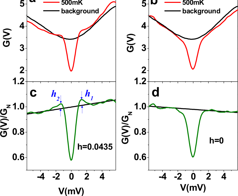
To compare the theoretical results with experiments, scanning tunneling spectroscopy (STS) measurements were performed at 500 mK on a set of three epitaxial NbN films grown on (100) oriented MgO substrates with different levels of disorder. NbN is an ideal system to investigate the SIT since disorder monotonically reduces mondal11 eventually giving rise to a non-superconducting state characterized by strong superconducting correlations chand12 . To avoid any surface contamination under exposure to air, these samples were grown in-situ in a chamber connected to the scanning tunneling microscope (STM). of the samples were measured from resistance vs. temperature measurement after completing the STS measurements. The samples investigated here had 1.65 K, 2.9 K and 6.4 K (defined as the temperature where dc resistance goes below our measurable limit) corresponding to an estimated 1.5, 1.8 and 2.7 respectively mondal11 ; chand12 . The thickness of all films was 50 nm which is much larger than the dirty limit coherence length mondal_jsnm of these films. Details of sample deposition and characterization have been reported in Refs. pratap_08 ; chand_09 ; chand12 .
STS measurements were performed using a home built scanning tunneling microscope operating down to 500 mK. The construction of the STM is similar to the one reported in ref. mondal11 , but is based on a 3He cryostat which allows us to go to lower temperatures. For each film tunneling conductance ( vs. ) was measured on 3232 grid over an area of 200200 nm. Two representative spectra on the sample with 1.65 K are shown in Figure 1 (a)-(b) (red lines). All the spectra show a prominent dip associated with the superconducting energy gap which adds to a broad temperature independent V-shaped background which extends up to high bias, arising from Altshuler-Aronov type electron-electron interactions mondal11 ; chand12 . At 8 K where superconducting correlations are destroyed the spectra only show the V-shaped background, which is spatially uniform within the noise level of our measurements (black lines in Fig. 1(a)-(b)). To isolate the feature associated with superconductivity from the background we divide the individual spectra obtained at low temperatures by the spatially average spectra obtained at 8K. The normalized spectra obtained in this way (Fig. 1(c)-(d)) do not show a significant variation in the magnitude of the superconducting energy gaps, but they show a large variation in the height of the coherence peaks. Since after correcting for background in most cases there is a small slope in the resulting spectrum, we fit a straight line passing through the high-bias region of the data to get the coherence peak height (Fig. 1(c)-(d)), and measure the peak heights with respect to this line for positive () and negative () bias. We define the average height of the coherence peaks at positive and negative bias over the normal state conductance, , as a measure of the local order parameter for our systemsacepe11 ; randeria11 . To make a quantitative comparison with the theoretical results we define for each sample the normalized local order parameter as
| (12) |
Thus, in analogy with the definitions (8)-(9), the quantity is always a real number between and .
III Numerical results
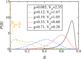
Let us start our analysis of the OPD with the results for the fermionic model (1). In Fig. 2 (a) we show the evolution of the OPD with the disorder amplitude . In agreement with previous workranderia01 , the generic behavior we observe, valid for all the parameters we considered, is an important broadening of the distribution which gets ultimately considerable weight near . As a consequence, the typical order parameter
| (13) |
and the average one , both marked by arrows in Fig. 2 (a), are very different, with . This means that the averaged quantity is governed by rare events and it is not representative of the typical behavior of the system. A similar behavior is found for the bosonic model studied by either CMF or 2D-CMF (see Fig. 2 (b) and (c)).
Note the presence of a cutoff at in the strongest disordered case: while at we observe a density bump, for the distribution falls down exponentially fast. This is due to the small probability of finding more than one neighboring site with large pairing amplitude at strong disorder. Therefore the order parameter , which is defined as an average of the 4 neighboring pairing amplitudes (9), can hardly have a value larger than (see also the discussion in Appendix after Eq. (20)). The same line of reasoning applies to the CMF and 2D-CMF with 4 replaced by , thus a cutoff at .
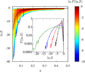
In Fig. 3 we show all our numerical results for the fermionic and bosonic models as a function of the coupling parameter . We plot to emphasize the structure of the OPD at low field value. The probability at each value for the given disorder strength is represented in a color plot, where the maximum of the distribution is located approximately at the typical value of the OP, . In 2D-CMF and CMF the SIT transition occurs at and , respectively, while in BdG the system remains superconducting right up to . As one can see in the insets of Fig. 3 (a) where is reported for some representative values, for CMF we recover the expected power-law decay with the universal (disorder-independent) exponent predicted in Refs. ioffe_prl10 ; feigelman_prb10 . However, such a power-law behavior is absent in the BdG and 2D-CMF results, where instead appears to be dominated by the low-field values, and to be strongly disorder-dependent. We notice that such a discrepancy between CMF and 2D results can hardly be attributed to the method itself: indeed, as we discuss in Appendix A, in 1D CMF and BdG give both with when which is in agreement with the exact critical behavior of the Ising model (3) dimitrova_jsm11 ; monthus_jpa12 .
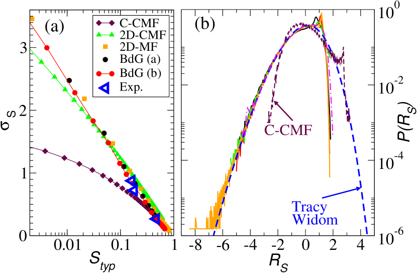
Such a distinction between CMF from one side and 2D results from the other can be made more quantitative by introducing as a scaling variable the logarithm of the OP, normalized to its variance . Indeed, as one can see in Fig. 4a, when disorder increases and scale in the same way in the 2D case, while within CMF tends to saturate at strong disorder. This result hints to a remarkable property of the OPD, that becomes evident when the above data are rescaled with the variable
| (14) |
As shown in Fig. 4b, provided that the coupling is small enough but still in the SC phase, all the data (except the ones for the CMF) collapse into one single curve (indeed, the left part of the rescaled distributions are hardly distinguishable). We verified that such scaling holds for smaller than the cutoff and in a wide range of parameters: as low as , different averaged densities, disorder strength and disorder distributions (box and gaussian distributions). It can also be noted that a value as low as is clearly not in the strong coupling regime where the fermionic Hubbard model (1) considered reduces essentially to hard-core bosons. Therefore, the universal collapse onto the bosonic result validates the bosonic scenario of Cooper pairing surviving the SIT. Another remark is that in all the cases represented, we have chosen the longitudinal size of the system sufficiently large to have converged to a size-independent distribution.
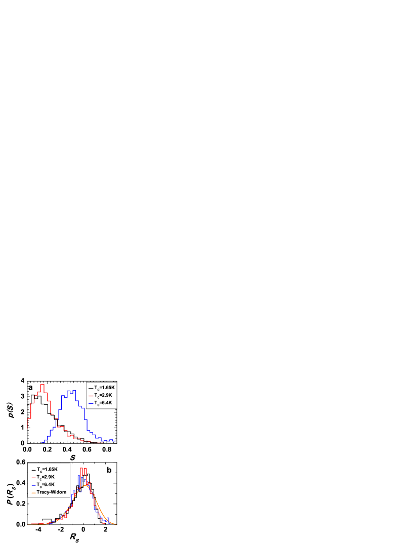
As it is shown in Fig. 4b the universal distribution followed by the rescaled data is well approximated by the Tracy-Widom distributionspohn with opposite asymmetry (ie TW where TW denotes the rescaled Tracy-Widom distribution). The relevance of the Tracy-Widom distribution in the insulating side of the SIT has been recently discussed in Refs. monthus_jsm12 ; monthus_jpa12 in connection with the physics of DP in finite dimensions. The connection between CMF on the Cayley tree and the DP physics had been already noticed in Refs. ioffe_prl10 ; feigelman_prb10 . It relies on a linearized form of the recursion equation (7), that one can expect to be approximately valid near the SIT where is small:
| (15) |
If one then studies the value at the root of the Cayley tree in response to infinitesimal fields at the boundary, one can write down as the sum over all the paths going from the root to the boundary. One then sees that is exactly the partition function of a directed polymer on a tree with edge energies at temperature . Such an analogy allows one to infer ioffe_prl10 ; feigelman_prb10 that at the system is always in the so-called localized phase of the DP problem, or equivalently in a phase with spontaneously broken replica symmetry (according to the language of Refs. ioffe_prl10 ; feigelman_prb10 ) where only a small number of paths contribute to the partition function. In finite dimension the equivalence between the cavity approximation and the DP is only approximate: nonetheless, as it has been discussed recently in Refs. monthus_jsm12 ; monthus_jpa12 , in the insulating phase the 2D-CMF approach described above is strictly connected to the DP problem. More specifically, in this regime the OP vanishes exponentially fast with the system size , but its fluctuations are tightly connected to the DP physics. Indeed, one finds that for a fixed scale :
| (16) |
where the variance scales like , being the droplet exponent of the DP in dimension, and a random variable of order following the GOE Tracy-Widom distribution. The droplet exponent decreases with increasing dimensionality and it vanishes identically on the Cayley tree, which then appears as an infinite-dimensional limit where the scaling (16) does not hold any more. When compared to our findings in Fig. 4b, one then finds that a similar scaling holds also in the SC phase, despite the fact that here the linearized recursion equation (15) used to map into the DP model is not well justified, since non-linear effects due to the finite order parameter are expected to be relevant. Thus, our finding that the OPD is related to the same Tracy-Widom distribution emerging in the DP problem is a completely unexpected result, which shows a posteriori that all the 2D methods and the DP problem seem to remain closely connected even in the SC side of the SIT transition 222The appearence of TW instead of TW is probably related to the non-linear effects which pose an upper bound to the distribution.
IV Universal scaling of the experimental order parameter distribution
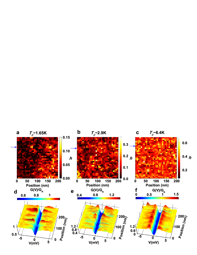
Figures 5(a)-(c) show the spatial variation of the OP over 200200 nm area in the form of intensity plot of for the three samples with different . We observe a smooth variation in over length scales of few tens of nanometers. This is further highlighted in figures 5(d)-(f) where we show a representative line scan of tunneling spectra for the three samples. To make a comparison with the theoretical results we plot in Fig. 6(a) the distribution of the normalized OP defined by Eq. (12). As disorder increases one observes a steady decrease in the maximum of the OPD along with a widening of the OPD, similar to the one reported in Ref. sacepe11 for InOx samples. This can be further quantified by computing as a function of the variance , which is found to follow the same trend as the theoretical 2D results (see Fig.4(a)). However, the most striking is that by introducing the scaling variable (14), all the three experimental OPD collapse into a single universal curve, despite their apparent difference when plotted in linear scale. In addition, the agreement with the universal Tracy-Widom distribution found in finite dimensions is very good as well. We can finally note that we do not observe a sharp cutoff on the experimental distributions as we observed in the numerical model data. On the other hand the experimental curves, although showing scaling among them, deviate from the Tracy-Widom distribution for high values of the order parameter. This can be due to a soft cutoff effect which breaks universality at large values of the order parameter. Alternatively it remains the possibility that experiments do scale to an universal curve but the Tracy-Widom distribution does not capture the behavior for large . More experimental and theoretical work would be needed to clarify this issue.
V Conclusion
In summary we have shown both theoretically and experimentally that the SC state at the verge of the SIT transition is characterized by a universal behavior of the OPD. The relevant scaling variable is the logarithm of the OP normalized to its variance. The latter diverges as the SIT is approached, unless the problem is studied on an infinite-dimensional lattice as the Caley tree, explaining the lack of such universality within the CMFioffe_prl10 ; feigelman_prb10 . The universal OPD shares a pronounced similarity with the Tracy-Widom distribution, whose role in the disordered phase of the random Ising model has been recently discussed within the mapping into the directed-polymer model in finite dimensionsmonthus_jsm12 ; monthus_jpa12 . Within such a mapping additional predictions have been made, as e.g. the divergence of the dynamical critical exponent as the SIT is approachedmonthus_jpa12 . This could be tested experimentally by the critical scaling of the superconducting fluctuations at , as done recently in other systemsarmitage . While the critical properties of real systems at the SIT should ultimately belong to the universality class, at intermediate disorder further experimental and theoretical investigation of these predictions will further clarify the relevance of the directed-polymer physics on the SIT.
VI acknowledgments
We would like to thank John Jesudasan and Vivas Bagwe for helping with the experiments and Subash Pai from Excel Instruments, Mumbai for continuous technical support. L.B. acknowledges partial financial support by MIUR under FIRB2012(RBFR1236VV). G.L. is supported by the EU through a Marie Curie Fellowship, FP7-PEOPLE-2010-IEF (project number 272268).
Appendix A Numerical and analytical results in 1D
In the present appendix we will show that the differences in the OPD between the CMF and the 2D results presented in the paper are not due to the underlying approximations but can be ascribed to the different lattice structures. Indeed, in one dimension, where the Cayley-tree lattice reduces to the usual 1D chain, both BdG and CMF approaches lead to the same behavior of the OPD.
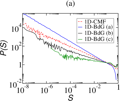
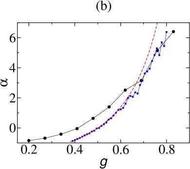
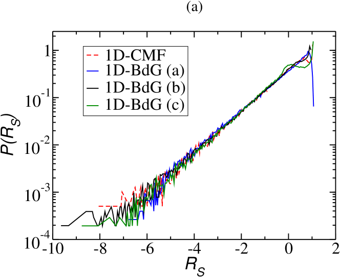
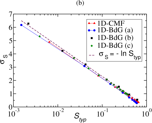
In Fig. 7 we report our results for the OPD within the Hubbard model and CMF in 1D. As one can see, has an universal power-law shape for low values of with of the order of the effective coupling : , with an exponent which depends on and goes from some positive value at large (ie for small disorder amplitude ) to when with BdG, or within CMF. By universal we mean that changing the parameters of the Hubbard model (averaged density , interaction strength and disorder strength ) does not affect the power law character but only the exponent . On the contrary, for large values of , the shape of the distribution is parameter dependent. In this respect the present 1D results demonstrate the equivalence between the BdG approach and the CMF when the lattice structure is the same. Moreover, such a behavior differs from the universal power-law behavior that would be expected by extending the result of Ref. ioffe_prl10 ; feigelman_prb10 up to .
Once established the equivalence between the BdG and CMF results, let us resort to the latter approach to understand analytically the power-law evolution near the SIT. Let us start from the recursive CMF equation in 1D, that is simply given by:
| (17) |
From Eq. (17) one can derive the following recursive relation for the OPD at zero temperature ( since in 1D):
| (18) |
Since the variable is independent of due to the recursive character of the approach, one can integrate it explicitly. Then one should distinguish whether . For small values of , one can approximate (18) by . Looking for a solution as a power law: , one obtains the condition:
| (19) |
whose non-trivial solution reproduces very well the numerical data of the CMF equation in 1D (see figure 7 (b)). For large , one finds
| (20) |
Note the singularity of the distribution at the cutoff . For this singularity translates into a density bump for at .
As we already discussed for the 2D case in Sec. III, also in 1D all the curves can be rescaled to an universal OPD by introducing the variable , where as before and , see Fig. 8. Also this result can be understood analytically by assuming that the form for the distribution of the order parameter holds at all values. Indeed in this case it is trivial to compute
| (21) |
which demonstrates that also in 1D both and increase as the SIT is approached. Within the same assumption we can also derive explicitly the distribution of the variable , given by:
| (22) | |||||
On the basis of the above relation (21) we have that and so that
| (23) |
References
- (1) P.W.Anderson, J. Phys. Chem. Solids 11, 26-30 (1959).
- (2) A.M.Goldman and N.Marković, Phys. Today 51, 39 (1998).
- (3) V. F. Gantmakher, Theory of Quantum Transport in Metallic and Hybrid Nanostructures, edited by A. Glatz et al. (Springer, New York, 2006), p. 83.
- (4) B. Sacépé, C. Chapelier, T. I. Baturina, V. M. Vinokur, M. R. Baklanov, M. Sanquer, Nature Communications 1, 140 (2010).
- (5) M. Mondal, A. Kamlapure, M. Chand, G. Saraswat, S. Kumar, J. Jesudasan, L. Benfatto, V. Tripathi, and P. Raychaudhuri, Phys. Rev. Lett. 106 047001 (2011).
- (6) B. Sacépé, C. Chapelier, T. I. Baturina, V. M. Vinokur, M. R. Baklanov, M. Sanquer, Nature Communications 1, 140 (2010).
- (7) M. Chand, G. Saraswat, A. Kamlapure, M. Mondal, S. Kumar, J. Jesudasan, V. Bagwe, L. Benfatto, V. Tripathi, P. Raychaudhuri, Phys. Rev. B85, 014508 (2012).
- (8) Y. Noat, T. Cren, C. Brun, F. Debontridder, V. Cherkez, K. Ilin, M. Siegel, A. Semenov, H.-W. Hübers, D. Roditchev, arXiv:1205.3408.
- (9) For a recent review see e.g. M. V. Feigel’man, L. B. Ioffe, V. E. Kravtsov, and E.Cuevas, Annals of Physics 325, 1368 (2010) and references therein.
- (10) M. Ma and P. A. Lee, Phys. Rev. B 32, 5658 (1985).
- (11) A. Ghosal, M. Randeria and N. Trivedi, Phys. Rev. B65, 014501 (2001).
- (12) M. V. Feigel’man, L. B. Ioffe, V. E. Kravtsov, and E. A. Yuzbashyan Phys. Rev. Lett. 98, 027001 (2007).
- (13) K. A. Matveev and A. I. Larkin, Phys. Rev. Lett. 78, 3749 (1997).
- (14) Y Dubi, Y. Meir and Y. Avishai, Nature 449, 876 (2007).
- (15) Y Dubi, Y. Meir and Y. Avishai, Phys. Rev. B78, 024502 (2008).
- (16) K. Bouadim, Y. L. Loh, M. Randeria and N. Trivedi, Nature Physics 7, 884 (2011).
- (17) G. Seibold, L. Benfatto, C. Castellani and J. Lorenzana, Phys. Rev. Lett. 108, 207004 (2012).
- (18) M. P. A. Fisher, G. Grinstein and S. M. Girvin, Phys. Rev. Lett. 64, 587 (1990).
- (19) L. B. Ioffe and M. Mézard Phys. Rev. Lett. 105, 037001 (2010).
- (20) M. V. Feigel’man, L. B. Ioffe, and M. Mézard Phys. Rev. B82, 184534 (2010).
- (21) O. Dimitrova, M. Mézard, J. Stat. Mech. (2011) P01020.
- (22) C. Monthus and T. Garel, J. Stat. Mech. (2012) P01008
- (23) C. Monthus and T. Garel, J. Phys. A: Math. Theor. 45, 095002 (2012)
- (24) P.G. de Gennes, Superconductivity in Metals and Alloys (Benjamin, New York, 1966).
- (25) B. Srinivasan, G. Benenti and D. L. Shepelyansky, Phys. Rev. B66, 172506 (2002)
- (26) M. Mondal, A. Kamlapure, S. C. Ganguli, J. Jesudasan, V. Bagwe, L. Benfatto and P. Raychaudhuri, Scientific Reports 3, 1357 (2013).
- (27) S. Robaszkiewicz, R. Micnas, and K. A. Chao, Phys. Rev. B23, 1447 (1981)
- (28) M. Prähofer and H. Spohn, Phys. Rev. Lett. 84, 4882 (2000)
- (29) B. Derrida and H. Spohn, J. Stat. Phys. 51, 817 (1988)
- (30) The 3He refrigerator based STM used in the present work, is similar in design to the one reported earlier in Ref. mondal11 .
- (31) M. Mondal, M. Chand, A. Kamlapure, John Jesudasan, V.C. Bagwe, S. Kumar, G. Saraswat, V. Tripathi and P. Raychaudhuri, J. Supercond Nov Magn 24, 341 (2011).
- (32) S. P. Chockalingam, M. Chand, J. Jesudasan, V. Tripathi and P. Raychaudhuri, Phys. Rev. B 77, 214503 (2008).
- (33) M. Chand, A. Mishra, Y. M. Xiong, A. Kamlapure, S. P. Chockalingam, J. Jesudasan, V. Bagwe, M. Mondal, P. W. Adams, Vikram Tripathi, and P. Raychaudhuri, Phys. Rev. B 80, 134514 (2009).
- (34) S. P. Chockalingam, M. Chand, A. Kamlapure, J. Jesudasan, A. Mishra, V. Tripathi and P. Raychaudhuri Phys. Rev. B 79, 094509 (2009).
- (35) The background also displays an asymmetry between posive and negative bias(not accounted for in Altshuler-Aronov theory) which was also observed in NbN/insulator/Ag planar tunnel junctionspratap09 . This asymmetry does not appear in Ref. mondal11 ; chand12 because the background slope was removed while aquiring the data.
- (36) The superconducting energy gap is estimated from the position of the coherence peaks for the first kind of spectra, and from the onset voltage of the sharp decrease in tunneling conductance in the second kind of spectra.
- (37) L.S.Bilbro et al. Nature Phys. 7, 298 (2011).
- (38) D. S. Fisher and D. A. Huse, Phys. Rev. B 43, 10728 (1991).
- (39) M. Mézard, J. Phys. I. (France) 51, 1831 (1990).
- (40) M. Sales and H. Yoshino, Phys. Rev. E 65, 066131 (2002).
- (41) E. Brunet and B. Derrida, Phys. Rev. E 61, 6789 (2000).