Common Patterns of Energy Flow and Biomass Distribution on Weighted Food Webs

Abstract

Weights of edges and nodes on food webs which are available from the empirical data hide much information about energy flows and biomass distributions in ecosystem. We define a set of variables related to weights for each species $i$, including the throughflow $T_{i}$, the total biomass $X_{i}$, and the dissipated flow $D_{i}$ (output to the environment) to uncover the following common patterns in 19 empirical weighted food webs: (1) DGBD distributions (Discrete version of a Generalized Beta Distribution), a kind of deformed Zipf’s law, of energy flow and storage biomass; (2) The allometric scaling law $T_{i}\propto X_{i}^{\alpha}$, which can be viewed as the counterpart of the Kleiber’s $3/4$ law at the population level; (3) The dissipation law $D_{i}\propto T_{i}^{\beta}$; and (4) The gravity law, including univariate version $f_{ij}\propto(T_{i}T_{j})^{\gamma}$ and bivariate approvement $f_{ij}\propto T_{i}^{\gamma_{1}}T_{j}^{\gamma_{2}}$. These patterns are very common and significant in all collected webs, as a result, some remarkable regularities are hidden in weights.

1 Introduction

Complex network is a useful tool to study interactions and relationships between components of a complex system(Watts and Strogatz, 1998; Albert and Barabasi, 2002). In ecology, complex network models are used in many ways, including representing trophic interactions in food webs(Montoya and Sole, 2002; Dunne et al., 2002; Williams et al., 2002; Berlow et al., 2004; Emmerson and Raffaelli, 2004) and energy-matter flux in ecosystems(Odum, 1988; Finn, 1976; Szyrmer and Ulanowicz, 1987; Higashi, 1986; Higashi et al., 1993; Baird and Ulanowicz, 1989; Fath and Patten, 1999). Some common patterns, such as the “two degrees separation”(Williams et al., 2002) and skewed or power law degree distributions(Dunne et al., 2002), are found on binary food webs. However, these studies never considered weights, which may hide important information of energy flux transferred between different species(Zhang and Guo, 2010).

Weights on edges and nodes stand for energy-matter flux between two compartments and biomass on each unit respectively(Higashi et al., 1993). Interestingly, Lindeman (1942) and Odum (1988)’s seminal works on food webs are all based on weighted networks. Patten (1985) et al. further developed a systematic method called environ analysis to uncover some hidden information in energy flows on networks. Besides the common phenomena found in earlier literatures including the hierarchical trophic structure and pyramid of biomass distribution(Odum, 1983; Odum et al., 2004), some quantitative and ubiquitous patterns such as dominant indirect effects(Higashi et al., 1993), network amplification(Patten et al., 1990), network homogenization(Patten et al., 1990), pathway proliferation(Patten, 1985; Borrett et al., 2007) and network synergism(Patten, 1992) are found by environ analysis in various food webs(Fath and Patten, 1999).

Metabolic theory is one of the greatest progresses in ecology in recent years which can be incorporated into food web studies(Brown, 2004). Several universal patterns or laws related to body size are discovered in the last two decades(Brown and West, 2000; West and Brown, 2005). For example, the three quarters power law relationship between metabolism and body mass (Kleiber’s law) is one of the most fundamental laws in metabolic theory(Kleiber, 1932). Some ecologists also tried to link these patterns to trophic structures(Nee et al., 1991; Loeuille and Loreau, 2006; Jennings and Mackinson, 2003; Damuth, 1981; Allen et al., 2002), including the energetic equivalence rule(Allen et al., 2002; Loeuille and Loreau, 2006); the trivariate relationship among body mass, trophic level and energy flows(Cohen et al., 2003). Nevertheless, some simple but important relations, say, biomass v.s. throughflow of each species, throughflow v.s. input flow and output flow are seldom addressed by these previous studies.

In parallel with these studies in ecology, the complex network community also started to pay attention to weight information of networks in recent years(Barrat et al., 2004; Almaas et al., 2004; Serrano et al., 2009; Tumminello et al., 2005). By incorporating the statistical mechanics method and random graph theory, weighted network analysis also revealed a series of universal patterns in various weighted networks, e.g. air traffic networks(Barrat et al., 2004; Guimera et al., 2005), metabolism networks(Almaas et al., 2004), world trade web(Bhattacharya et al., 2007) and stock-sharing networks of companies(Vitali et al., 2011), etc. The new found common patterns include: long tailed distribution of node intensity (total weights of each node), the power law relationship between degree and intensity(Barrat et al., 2004), the so called gravity law(Anderson, 2011; Erlander and Stewart, 1990; Krings et al., 2009), and so forth. Energy flow networks in ecosystem no doubt are also weighted networks though the weight here has the special meaning, i.e. the energy flux transferred by different species(Zhang and Guo, 2010). Therefore, it is reasonable to conjecture that the patterns found in other weighted networks should be also suitable for the weighted food webs. This paper tries to apply the approaches developed by complex weighted network studies to the energy flow networks in ecology.

This paper is organized as follows: in Section 2, we introduce some basic variables including the weights of edges and nodes. And also, the so called DGBD (Discrete version of a Generalized Beta Distribution)(Martínez-Mekler et al., 2009) curve which can fit the weights distributions better than the traditional curves is introduced. After that, the results of biomass and energy flow distributions and several universal relationships including the allometric law at the population level, the dissipation law and the gravity law on 19 weighted food webs are shown in Section 3. After that, several interesting problem around these common patterns are discussed. We found an interesting negative linear relationship between exponents of fitted DGBD distributions in energy flow, biomass and degree distributions (see Section 4.1). And the mathematical relations among the scaling exponents are derived. Finally, the connection with the abundance-body mass relationship is discussed in Section 4.

2 Materials and Methods

2.1 Data source

We have investigated 19 food webs in different ecological environments. The food web information includes node (species or non-living compartment), node weight (biomass of a node), edge (energy flow relationship but not feeding relationship), and edge weight (the amount of energy flow from node $i$ to $j$). The energy flow between two nodes was measured as the unit volume flow of the carbon element into or out of the node (the unit is gC/$m^{2}$/year)). The biomass stands for the total mass of living biological organisms of a species in a certain period of time and per unit volume. Customarily it was also measured by carbon content (the unit is gC/$m^{2}$) (Baird and Ulanowicz, 1989). These food webs’ information is obtained from the online database, which is based on the published papers(Baird et al., 1998; Baird and Ulanowicz, 1989; Ulanowicz, 1986; Almunia et al., 1999; Monaco and Ulanowicz, 1997; Hagy, 2002). In Table 1, we list the name and the number of nodes $N$ and edges $E$ of each web.

Table 1: Empirical food webs and their topological properties

($N$ stands for the number of vertices of the network and $E$ is the number of edges. The webs are sorted by $E$.) Food web Abbre. $N$ $E$ Crystal River Creek (Delta Temp) CrystalD 23 60 Crystal River Creek (Control) CrystalC 23 81 Chesapeake Bay Mesohaline Net Chesapeake 38 122 Lower Chesapeake Bay in Summer ChesLower 36 115 Middle Chesapeake Bay in Summer ChesMiddle 36 149 Upper Chesapeake Bay in Summer ChesUpper 36 158 Narragansett Bay Narragan 34 158 Lake Michigan Michigan 38 172 St. Marks River (Florida) StMarks 53 270 Mondego Estuary - Zostrea site Mondego 45 348 Cypress, Wet Season CypWet 70 545 Cypress, Dry Season CypDry 70 554 Everglades Graminoids, Dry Season GramDry 68 793 Everglades Graminoids, Wet Season GramWet 68 793 Mangrove Estuary, Dry Season MangDry 96 1339 Mangrove Estuary, Wet Season MangWet 96 1440 Florida Bay, Wet Season BayWet 127 1938 Florida Bay, Dry Season BayDry 127 1969 Florida Bay Florida 127 1938

2.2 Basic variables

Our work is based on the flux matrix of a weighted food web. An ecological energy flow network is a weighted directed graph that represents relationships of ecological energy transfer between species. This graph can be represented by a flux matrix:

$$F_{(N+2)\times(N+2)}\;=\{f_{ij}\}_{(N+2)\times(N+2)},\;\;\;\forall i,j\in[0,N+1]$$ (1)

where $f_{ij}$ is the energy flow from species $i$ to $j$. Two special nodes representing environment (node $0$ and node $N+1$) are added to the web. Node $0$ denotes the source of energy flow, whereas node $N+1$ represents the sink. The dissipative and exported energy flow to the node $N+1$. Therefore, there are totaly $(N+2)\times(N+2)$ entries. The flux matrix $f_{(N+2)\times(N+2)}$ can be read from the original weighted food webs(Baird et al., 1998; Baird and Ulanowicz, 1989; Ulanowicz, 1986; Almunia et al., 1999; Monaco and Ulanowicz, 1997; Hagy, 2002).

We can calculate the total through flow of any given node $i$ according to the flux matrix $F_{(N+2)\times(N+2)}$ (see figure 1). This value is also called node strength in complex weighted network studies (Almaas et al., 2004). Because the network is always balanced, we need only to calculate the efflux of each node as $T_{i}$,

$$T_{i}\;=\sum_{j=1}^{N+1}f_{ij}=\sum_{j=0}^{N}f_{ji},\;\;\;\forall i\in[1,N].$$ (2)

Figure 1: An Illustration of variables

In addition, we define another variable to represent the weight of a node $X_{i}$, indicating the biomass of $i$. This information is also available from the original weighted food webs.

$D_{i}$ is the dissipated flow to the environment (node $N+1$) from species $i$: $f_{i,N+1}$ (see figure 1). The dissipation flow includes the flows of output and respiration.

$k_{i}^{in}$ and $k_{i}^{out}$ are in-degree and out-degree, i.e., the number of inward edges (excluding edges from the source) and outward edges (excluding the edges to the sink) of $i$ respectively. In the example network in figure 1, $k_{i}^{in}=3$ and $k_{i}^{out}=1$.

2.3 Distributions and DGBD curves

We will study the distributions of $T_{i}$, $X_{i}$, $k_{i}^{in}$ and $k_{i}^{out}$ in any empirical food web. Instead of giving the empirical density or distribution function (Zhang and Guo, 2010), we use the rank-ordered curve to show the distributions of these variables. For example, if we have a small food web with 5 species, and their biomass values are $\{100,19,200,5,1\}$ gC/$m^{2}$. A sequence of biomass values in a decreasing order can be obtained: $\{200,100,19,5,1\}$. Then we plot this sequence on a coordinate with the horizontal axis as the rank value, namely $\{1,2,3,4,5\}$ and the vertical axis as the biomass values. So the final curve on this coordinate is the rank-ordered curve. The main advantage of adopting this curve is its simplicity for the calculation, as well as it contains the same information as the distribution function (Newman, 2005).

Then, we use the DGBD (Discrete version of a Generalized Beta Distribution) function to fit the rank-ordered curve:

$$Y(r_{i})=A\frac{(N+1-r_{i})^{a}}{r_{i}^{b}},\hskip 28.45274pta,b\geqslant 0$$ (3)

where, $Y(r_{i})$ is the value of the concerned variable ($T_{i}$ or $X_{i}$) of the node $i$, and $r_{i}$ is the decreasing order of $i$ ranked by $Y(r_{i})$ values. $N$ is the total number of nodes in the food web. $A,a,b\geq 0$ are parameters to be estimated. $A$ stands for the magnitude of flow or biomass in this food web which is dependent on the measurement units. $a$ and $b$ are exponents of power laws in the tail and head part of the curves respectively. If we set $a=0$, then formula (4) becomes $Y(r_{i})=A/{r_{i}^{b}}$, which is the famous Zipf’s law (Newman, 2005). However, the classic Zipf’s law is not always the best choice for fitting empirical data due to the large deviations in the tail part of the rank-ordered curves (Martínez-Mekler et al., 2009). This disadvantage can be mended by introducing a new exponent $a$ in the DGBD fitting. Previous study shows that formula (4) can fit lots of empirical data very well (Martínez-Mekler et al., 2009).

Notice that, if we set $a=0$ in equation 4, then the rank-ordered curve of a variable $Y$ follows Zipf’s law with the exponent $b$. Therefore, the density function of the random variable $Y$ is a power law with the exponent $1/b+1$ due to the one-one correspondence between the rank-ordered function and probability density function(Newman, 2005). So, DGBD curve is capable to not only fit those data with power law tails (note that the tail part of the density function is just the head part of the rank-ordered curve) but also the data with an obvious deviation from power laws by tuning the extra exponent $a$ (figure 2).

Figure 2: Different shapes of rank-ordered curves with different $a$ and $b$ under the same $A=1$ and $N=100$. (a) Rank-ordered curves on a linear-log plot; (b) The same rank-ordered curves on a log-log plot; (3) The probability density curves of the same four groups of data on a log-log plot

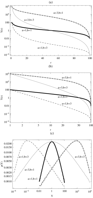
As shown in figure 2, different combinations of $a$ and $b$ correspond different shapes of the distribution curve. Exponent $b$ is the slope of the head part of the rank-ordered curve in figure 2 (b) as well as the tail part of the probability density curve in figure 2 (c). Therefore, we say $b$ indicates the heterogeneity of $Y$ distributing for the large species. On the other hand, $a$ indicates the unevenness of the tail part of the rank-ordered curve (figure 2 (a) and (b)) as well as the head part of the probability density curve (figure 2 (c)). As $a$ increases, the tail of the rank-ordered curve drops very fast so that the $Y$ sharing heterogeneity in the small species is very large.

We mainly adopt OLS (Ordinary Linear Square regression) method to fit DGBD curves and other power law relationships. We can take logarithmic on equation 4 to derive:

$$\log(Y(r_{i}))=\log(A)+a\log(N+1-r_{i})-b\log(r_{i}).$$ (4)

Thus, $\log(Y(r_{i}))$ depends on two variables $\log(N+1-r_{i})$ and $\log(r_{i})$ so that the bivariate linear regression method can be used to derive the coefficients $\log(A),a$ and $b$.

3 Results

3.1 The DGBD distributions

We obtain the distribution of $T_{i},X_{i},k_{i}^{in}$ and $k_{i}^{out}$ for each of the 19 empirical food webs, and fit them by DGBD curves. One selected food web as an example is plotted in figure 3.

From figure 3, we know the curves can be divided into three parts by two inflexion points, and each part obeys independent logarithmic decreasing behavior. Obviously, the head and tail parts of the curve have much steeper slopes than the middle part. The local slope of the curves indicates the heterogeneities of the throughflow distribution. In other words, the larger the absolute value of slope is, the higher the degree of heterogeneity of a vertex correspondingly is. Therefore, we can conclude that the nodes in the heads and tails are more heterogeneous than the ones in the middle.

Figure 3: Rank-ordered distributions and DGBD fittings of $T_{i},X_{i},k_{i}^{out}$ and $k_{i}^{in}$ for Mangwet food web. The indications of 1st, 2nd and 3th level species in the legend represent the first, second and third trophic level species in the food web.

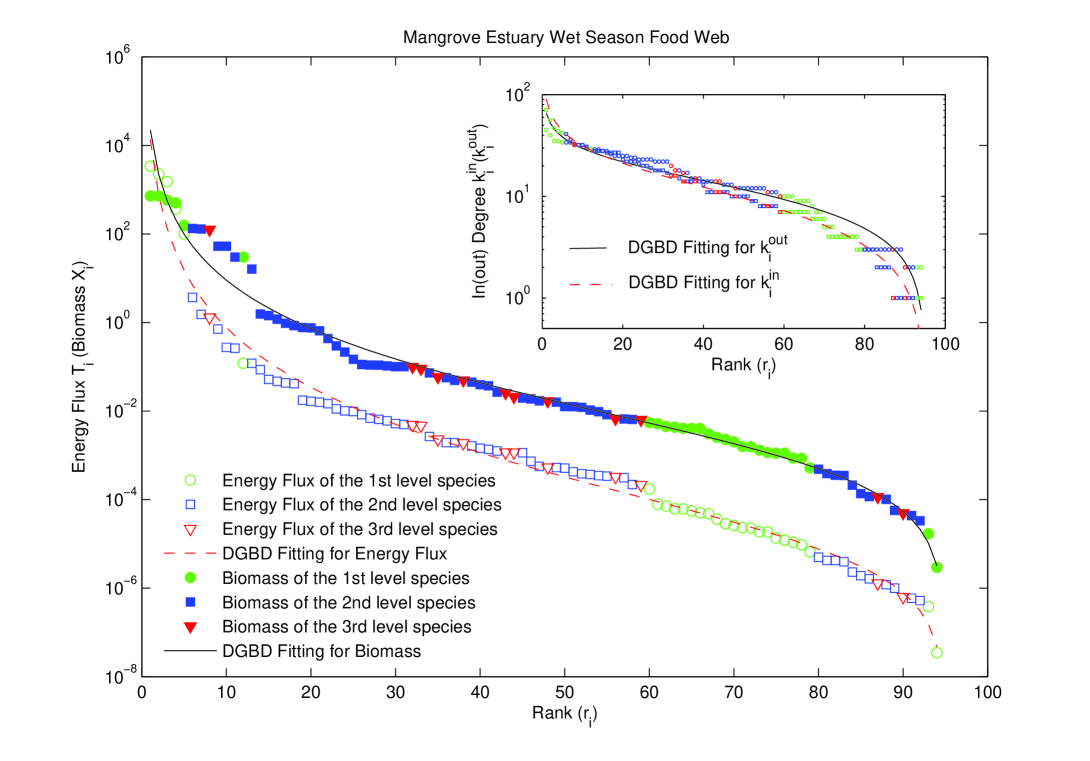
In figure 3, we distinguish nodes by their trophic levels. Green circles, blue squares, and red triangles represent the first, second and third trophic level species respectively. It is observed that nodes of first trophic level locate both at the head and tail parts, while most of the second level species locate at the middle part, and most third trophic level species are in the middle or tail parts of the curve. This distribution pattern of species on different trophic levels is similar for all large food webs (the food webs below Michigan web in table 1). We may conclude that the distribution of throughflow on the second trophic level is much more even than the first and third trophic levels. The inset figure of figure 3 plots the rank-ordered distributions of in-degree and out-degree of all edges. These two curves have the similar shape with the energy flow and biomass distributions.

Table 2: DGBD fitting parameters for different variables

(The webs are sorted by their number of edges.) Web $a_{T_{i}}$ $b_{T_{i}}$ $R_{T_{i}}^{2}$ $a_{X_{i}}$ $b_{X_{i}}$ $R_{X_{i}}^{2}$ $a_{k_{i}^{out}}$ $b_{k_{i}^{out}}$ $a_{k_{i}^{in}}$ $b_{k_{i}^{in}}$ CrystalD $0.45$ $3.96$ $0.96$ $0.00$ $4.21$ $0.97$ $0.00$ $0.69$ $0.00$ $0.98$ CrystalC $0.76$ $3.41$ $0.97$ $0.24$ $3.89$ $0.95$ $0.20$ $0.56$ $0.35$ $0.71$ Chesapeake $2.93$ $1.54$ $0.94$ $1.70$ $2.17$ $0.99$ $0.23$ $0.50$ $0.19$ $0.73$ ChesLower $10.02$ $0.00$ $0.80$ $5.53$ $0.75$ $0.85$ $0.68$ $0.17$ $0.15$ $0.88$ ChesMiddle $6.88$ $0.00$ $0.83$ $3.42$ $0.77$ $0.87$ $0.55$ $0.25$ $0.40$ $0.63$ ChesUpper $4.77$ $0.00$ $0.72$ $3.42$ $0.86$ $0.88$ $0.61$ $0.16$ $0.37$ $0.70$ Narragan $0.80$ $2.54$ $0.93$ $0.16$ $1.88$ $0.93$ $0.21$ $0.47$ $0.41$ $0.56$ Michigan $6.59$ $0.81$ $0.95$ $4.80$ $0.18$ $0.89$ $0.51$ $0.47$ $0.45$ $0.45$ StMarks $1.25$ $1.33$ $0.99$ $0.94$ $2.14$ $0.98$ $0.59$ $0.38$ $0.54$ $0.40$ Mondego $3.36$ $1.70$ $0.97$ $1.41$ $2.43$ $0.99$ $0.57$ $0.26$ $0.48$ $0.94$ Cypwet $2.74$ $2.63$ $0.97$ $3.03$ $4.23$ $0.98$ $0.41$ $0.56$ $0.62$ $0.66$ Cypdry $2.34$ $2.36$ $0.95$ $2.51$ $3.99$ $0.98$ $0.43$ $0.52$ $0.63$ $0.66$ Gramdry $2.08$ $3.18$ $0.97$ $2.75$ $2.75$ $0.97$ $0.34$ $0.43$ $0.67$ $0.54$ Gramwet $3.03$ $2.94$ $0.97$ $3.74$ $2.40$ $0.97$ $0.34$ $0.43$ $0.67$ $0.54$ Mangdry $1.51$ $3.22$ $0.97$ $1.41$ $4.08$ $0.98$ $0.66$ $0.32$ $0.79$ $0.42$ Mangwet $1.67$ $3.32$ $0.98$ $1.63$ $4.18$ $0.99$ $0.66$ $0.32$ $0.79$ $0.43$ Baywet $1.65$ $2.80$ $0.97$ $2.26$ $2.40$ $0.99$ $0.74$ $0.40$ $0.97$ $0.25$ Baydry $1.62$ $2.63$ $0.98$ $2.24$ $2.28$ $0.98$ $0.75$ $0.39$ $0.97$ $0.25$ Florida $1.65$ $2.80$ $0.97$ $2.26$ $2.40$ $0.99$ $0.74$ $0.40$ $0.97$ $0.25$

In Table 2, we list all the fitted parameters and $R^{2}$s of DGBD for the 19 webs. Only the exponents of $a$ and $b$ are shown in the table because $A$ representing the magnitude of throughflow or biomass is relatively unimportant. By comparing different rows, we know that the food webs with more edges can be better fitted by DGBD curves because their $R^{2}$s are larger. Notice that there are three food webs (ChesLower, ChesMiddle and ChesUp) having exponents $b_{X_{i}}=0$ and one web (CrystalD) having exponents $a_{X_{i}},a_{k_{i}^{in}},a_{k_{i}^{in}}=0$. That means these webs are anomalous and reach the extremal cases of DGBD curves. However the $R^{2}$’s of the the fitting curves are also very high.

The last four columns show the DGBD fittings of in and out degrees. An obvious trend is the exponent $a_{k_{i}}$ increases, however $b_{k_{i}}$ decreases with the size of the food web. That indicates the number of connected species distributes on different nodes more evenly in small food webs and the average degrees increase with the size of the web.

3.2 Allometric scaling laws at the population level

According to the similarity between the distribution curves of $T_{i}$ and $X_{i}$ in figure 3, we guess there may exist a connection between variables $X_{i}$ and $T_{i}$. The log-log plot of these two variables shows that the relationship between $X_{i}$ and $T_{i}$ is actually a power law:

$$T_{i}\propto X_{i}^{\alpha},$$ (5)

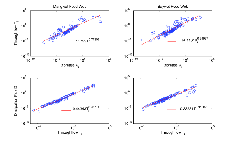
where exponent $\alpha$ is a parameter to be estimated for each food web. As shown in upper row in figure 4, the sample points aggregate around their fitted lines very well. This relationship is ubiquitous for all 19 food webs as shown in Table 3. We use the ordinary linear regression method to find the best fitting lines (Table 3). And most $R^{2}$’s are larger than $0.8$. The $R^{2}$’s and exponents decrease with the scale of the network because the statistical significance increases with the number of samples.

Figure 4: Power law relationships of $T_{i}$ v.s. $X_{i}$ and $D_{i}$ v.s. $X_{i}$. The original data points as well as the OLS fittings are shown on the log-log coordinate

Table 3: Fitting exponents and goodness of power law relationships

( The webs are sorted by their number of edges.) Web $\alpha$ $R_{allo}^{2}$ $c$ $\beta$ $R_{diss}^{2}$ $\gamma$ $R_{gra}^{2}$ $\gamma_{1}$ $\gamma_{2}$ $R_{bi}^{2}$ $\eta$ CrystalD $0.98$ $0.90$ $0.67$ $0.96$ $1.00$ $0.63$ $0.70$ $0.57$ $0.75$ $0.74$ 11.5 CrystalC $0.92$ $0.88$ $0.68$ $0.96$ $0.99$ $0.53$ $0.65$ $0.50$ $0.57$ $0.65$ 2.125 Chesapeake $1.03$ $0.75$ $0.50$ $0.99$ $0.98$ $0.68$ $0.84$ $0.62$ $0.77$ $0.85$ -9.33 ChesLower $1.75$ $0.91$ $0.49$ $0.95$ $0.99$ $0.70$ $0.75$ $0.61$ $0.84$ $0.76$ -1.33 ChesMiddle $1.58$ $0.82$ $0.47$ $0.88$ $0.85$ $0.67$ $0.77$ $0.60$ $0.78$ $0.78$ -1.43 ChesUpper $1.21$ $0.64$ $0.58$ $0.95$ $0.99$ $0.64$ $0.64$ $0.62$ $0.67$ $0.64$ -2.19 Narragan $1.17$ $0.55$ $2.05$ $0.81$ $0.94$ $0.54$ $0.81$ $0.49$ $0.60$ $0.81$ -2.47 Michigan $1.20$ $0.94$ $0.67$ $0.99$ $1.00$ $0.62$ $0.86$ $0.57$ $0.72$ $0.87$ -2.25 StMarks $0.69$ $0.70$ $0.43$ $0.99$ $0.95$ $0.68$ $0.74$ $0.76$ $0.56$ $0.75$ -0.19 Mondego $1.24$ $0.87$ $0.53$ $0.98$ $1.00$ $0.79$ $0.85$ $0.83$ $0.70$ $0.86$ -2.04 Cypwet $0.66$ $0.78$ $0.46$ $0.97$ $0.99$ $0.70$ $0.84$ $0.85$ $0.55$ $0.87$ -0.26 Cypdry $0.63$ $0.76$ $0.41$ $0.96$ $0.95$ $0.68$ $0.81$ $0.81$ $0.57$ $0.83$ -0.32 Gramdry $0.90$ $0.90$ $0.58$ $0.97$ $1.00$ $0.66$ $0.76$ $0.61$ $0.73$ $0.77$ 1.5 Gramwet $0.93$ $0.92$ $0.59$ $0.98$ $1.00$ $0.71$ $0.81$ $0.66$ $0.79$ $0.81$ 2.57 Mangdry $0.77$ $0.82$ $0.45$ $0.98$ $0.98$ $0.58$ $0.77$ $0.60$ $0.56$ $0.77$ 0.09 Mangwet $0.78$ $0.83$ $0.44$ $0.98$ $0.98$ $0.59$ $0.77$ $0.60$ $0.57$ $0.77$ 0.13 Baywet $0.87$ $0.81$ $0.33$ $0.92$ $0.95$ $0.62$ $0.79$ $0.67$ $0.54$ $0.80$ 0.92 Baydry $0.85$ $0.81$ $0.32$ $0.91$ $0.95$ $0.61$ $0.78$ $0.68$ $0.52$ $0.78$ 0.67 Florida $0.87$ $0.81$ $0.33$ $0.92$ $0.95$ $0.62$ $0.79$ $0.67$ $0.54$ $0.80$ 0.92

This specific scaling relationship reminds us the famous allometric scaling law (Brown, 2004; West and Brown, 2005; Banavar et al., 1999). Kleiber (1932) found that the metabolism and body size of an organism usually follows a ubiquitous power law relationship with an exponent around $3/4$. If we treat the whole population of a species as an integrated organism, then $T_{i}$ is its metabolism and $X_{i}$ is its body mass. Therefore, equation 5 can be viewed as the allometric scaling law at the population level. Nevertheless, unlike the universal Kleiber’s law for species, the allometric scaling exponents of population on food webs are not universal but fluctuate in between $[0.63,1.75]$.

3.3 Dissipation law

As pointed by the earlier ecological studies(Odum, 1983; Lindeman, 1942), a large fraction of energy flows dissipates to the environment in the whole ecosystem. The dissipated energy flow can be captured by the variable $D_{i}$ which is also available from the original data. Empirically, $D_{i}$ scales with throughflow $T_{i}$ in the following way:

$$D_{i}=cT_{i}^{\beta}.$$ (6)

Equation 6 is called dissipation law in this paper, where $c$ and $\beta$ are parameters to be estimated. We observe that the estimated exponents $\beta$ are all slightly smaller than 1 (see the 2nd row of figure 4 and the 4th 6th columns of table 3), therefore the dissipation rate (dissipation per throughflow) decreases with the throughflow of the species slightly. If $\beta=1$, $c$ is the average energy dissipation rate of the whole food web. Since the empirical exponents in table 3 are approaching to 1, the coefficient $c$’s are almost the dissipation rate of the specific food web. From table 3, we can read $c$’s are fractional numbers that are smaller than one except the food web Narragan whose exponent $\beta$ deviates 1 significantly.

3.4 Gravity Law

Although we have studied the ways of energy flows correlate with the biomass and dissipation, we still don’t know how the energy flows distribute among different pairs of species. Actually, the large throughflow nodes can exchange large energy flows. This effect is reflected by the so called gravity law, namely, the energy flow between $i$ and $j$ scales with the product of the total throughflows of $i$ and $j$, i.e.,

$$f_{ij}\propto(T_{i}T_{j})^{\gamma}.$$ (7)

This scaling relation is known as the gravity law in other complex systems. Researchers found the flows, say traffic flow or trade flow between cities or countries scales with $(m_{1}m_{2})^{\gamma}/d^{\tau}$, where $m_{i}$ is the size of the system (population of a city or GDP of a country) and $d$ is the distance between the two systems, $\gamma$ and $\tau$ are fitting exponents. In our case, the throughflow of each node $T_{i}$ is treated as the size of a node comparable to the population of a city. However, the distance $d$ has no correspondence because spatial information is not included in our food webs.

Figure 5: Univariate and bivariate gravity law of Mangwet food web. (a) The univariate scaling relationship $f_{ij}\propto(T_{i}T_{j})^{0.587}$; (b) The bivariate scaling relationship $f_{ij}\propto T_{i}^{0.6}T_{j}^{0.57}$. The original data points as well as the OLS fittings are shown on the log-log coordinate

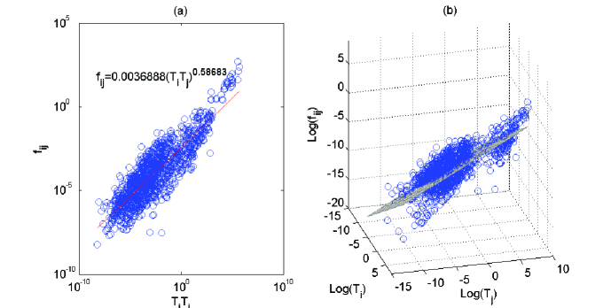
Figure 5(a) shows this phenomenon and the parameters are listed in the last two columns of table 3. This pattern is not as significant as the previous two patterns because the $R^{2}$’s are always smaller than $0.85$. From figure 5 (a), we could observe that there are several straight bands in the clusters of data points which indicates that the energy flow between two nodes $f_{ij}$ may be predicted by other variables rather than the product of $T_{i}$ and $T_{j}$.

As the studies in gravity laws, we suggest that the following bivariate scaling relation holds,

$$f_{ij}\propto T_{i}^{\gamma_{1}}T_{j}^{\gamma_{2}}.$$ (8)

Where, $\gamma_{1}$ and $\gamma_{2}$ are two estimated parameters. Figure 5 (b) shows this bivariate gravity law. All the estimated exponents $\gamma_{1}$, $\gamma_{2}$ and the corresponding $R^{2}$ are shown in the last 2nd, 3rd and 4th columns in table 3. The bivariate gravity law equation 8 can fit the original data better than equation 7 since the corresponding $R_{bi}^{2}$’s are slight higher than $R_{gra}^{2}$’s. Another interesting phenomenon observed from table 3 is that the exponent $\gamma_{2}$ is larger than $\gamma_{1}$ for small food webs but smaller than it for large food webs except Gramdry and Gramwet. We can conclude that the large energy flows prefer to link nodes with large throughflow in all food webs. The dependence of energy flow on the donator (prey) and receptor (predator) is asymmetric. As the energy flow along each edge increases, the energy throughflows of receptors increases faster than donators in small food webs. The speed of increasing of throughflows for donator is higher than receptors in large food webs.

All of these observed patterns of energy flows exhibit statistical significance and universality for all 19 empirical food webs.

4 Discussions

4.1 Relationships of exponents

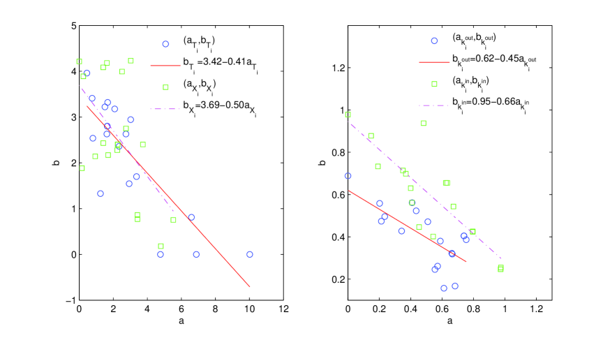
In section 3.1 and table 2, we have obtained a set of fitting exponents of DGBD curves. These exponents also have some patterns. It is observed from table 2 that exponents $a$ and $b$ have a negative correlation. The relationship is very clear once we plot the pairs of $(a,b)$ in one coordinate (see figure 6). We separate the $a,b$ exponents of $T_{i},X_{i}$ and the ones of $k_{i}^{out},k_{i}^{in}$ because the former has a wider range. However all these pairs of $(a,b)$ show the nearly linear relationship with similar negative slopes (the mean slope is $-0.5$) and statistical significance (the $R^{2}$’s of these relationships are all larger than $0.5$ except $k_{i}^{in}$).

We suppose this pattern reflects a kind of particular regularity of food webs since the similar phenomenon is never reported in previous studies(Martínez-Mekler et al., 2009). The negative correlation between exponents $a$ and $b$ implies a kind of complementarity between the heterogeneities of energy flow or biomass resources distributions at the head and tail part species on rank curves. As the heterogeneity of the small species increases, the unevenness of energy distribution in large species decreases.

Figure 6: The linear relationships of DGBD fitted exponents $a$ and $b$ in four distributions ($T_{i},X_{i},k_{i}^{out},k_{i}^{in}$). The $R^{2}$’s of the best fitting lines are $R_{T_{i}}^{2}=0.51,R_{X_{i}}^{2}=0.72,R_{k_{i}^{out}}^{2}=0.67,R_{k_{i}^{in}}^{2}=0.35$

Figure 7: The real relationship between $a_{T_{i}}(b_{T_{i}})$ and $a_{X_{i}}\alpha(b_{X_{i}}\alpha)$, and the predicted one (the 45 degree diagonal straight line).

Besides this pattern, other two interesting relationships between the exponents of distributions and power law relationships can be derived . We can write down the DGBD distributions of $T_{i}$ and $X_{i}$ in the following forms:

$$T_{i}\;=A_{T_{i}}\frac{(N+1-r_{i})^{a_{T_{i}}}}{r_{i}^{b_{T_{i}}}}.$$ (9)

and

$$X_{i}\;=A_{X_{i}}\frac{(N+1-r_{i})^{a_{X_{i}}}}{r_{i}^{b_{X_{i}}}}.$$ (10)

for each node $i$. As we have shown in section 3.2, $T_{i}$ and $X_{i}$ follow a power law relationship: equation (5). If we insert equation (9) and (10) into equation (5), we can easily derive the following equation:

$$\frac{(N+1-r_{i})^{a_{T_{i}}}}{r_{i}^{b_{T_{i}}}}\propto(\frac{(N+1-r_{i})^{a_{X_{i}}}}{r_{i}^{b_{X_{i}}}})^{\alpha}.$$ (11)

This should be satisfied for any $r_{i}$. So comparing the coefficients of the terms $(N+1-r_{i})$ and $r_{i}$, we can derive the following relationships.

$$a_{T_{i}}={a_{X_{i}}}{\alpha},$$ (12)

and

$$b_{T_{i}}={b_{X_{i}}}{\alpha}.$$ (13)

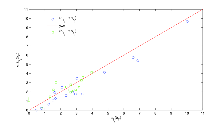
If these two relations hold for all food webs, the pairs of $(a_{T_{i}},\alpha a_{X_{i}})$ or $(b_{T_{i}},\alpha b_{X_{i}})$ in the empirical food webs should form a straight line with a 45 degree slope.

From Figure 7, the pairs of $(a_{T_{i}},\alpha a_{X_{i}})$ or $(b_{T_{i}},\alpha b_{X_{i}})$ concentrate around the predicted relationship with small deviations. That means the predicted relationships (equations 12 and 13) are almost correct for the empirical food webs. However, a systemic deviation from the predicted line exists for $(a_{T_{i}},\alpha a_{X_{i}})$ since all the data points are lower than the theoretical line. Therefore, we may underestimate the values of $a_{X_{i}}$ or overestimate $a_{T_{i}}$. The errors can not come from the estimation of $\alpha$ because the similar systemic deviation of $\alpha b_{X_{i}}$ is not observed. However the reasons for these errors are still mysteries for us.

4.2 Other possible patterns

Besides the common patterns shown in the previous texts, we have also investigated other possible patterns exhaustively. However they are either unclear or trivial.

For example, there is a power law relationship between node degree and strength in other weighted complex networks as shown in previous studies (Barrat et al., 2004). Although a positive correlation between the degree and strength can be observed in our food webs, this power law relation is not significant($R^{2}=0.22$).

The energy flow distributions for each node also obey DGBD curves, but this content is abandoned in the main text because it can not provide us more insights.

Another trivial scaling relationship is between the energy flow $f_{ij}$ and the product of biomass of the two species $X_{j}X_{j}$ because it is an obvious result from the scaling relationship in equation 7 and equation 5.

Finally, one may guess that a power law relationship between $k_{in}$ and $k_{out}$ must exist because of the similarity of the distribution curves in the inset of figure 2. However, their relations are not significant once we draw the pairs of $k_{in},k_{out}$ in one coordinate. Therefore, all the patterns we have selected are significant and nontrivial.

4.3 Abundance and Body Size

Body size is treated as a very fundamental observable in ecology because it determines other important variables of organisms including the trophic structure(Cohen et al., 2003; Brown, 2004; Brown and Gillooly, 2003). Cohen et al. (2003), Brown and Gillooly (2003) discussed the scaling relationship between abundance and body mass in food web. We may derive a relationship between abundance and body size from the scaling relation between throughflow and biomass of each node. Suppose the numeric abundance of species $i$ is $N_{i}$, the average body mass of $i$ is $M_{i}$, and its average energy metabolism is $F_{i}$. Then, according to the definitions,

$$X_{i}=N_{i}M_{i},$$ (14)

and

$$T_{i}=N_{i}F_{i}.$$ (15)

The Kleiber’s law links $M_{i}$ and $F_{i}$ as follows for any species $i$,

$$F_{i}\propto M_{i}^{3/4}.$$ (16)

So, insert these relations into equation 5, we have,

$$N_{i}\propto M_{i}^{\frac{3/4-\alpha}{\alpha-1}}.$$ (17)

Therefore, the scaling exponent between abundance and body size $\eta$ is:

$$\eta=\frac{3/4-\alpha}{\alpha-1}.$$ (18)

This exponent can be estimated according to the exponent $\alpha$ for any empirical food webs. The $\eta$ values are derived in the last column of Table 3. We can see that the exponent $\alpha$ may be either positive or negative which means the abundance may increase or decrease with body mass. This conclusion contradicts with our observations and the exponent deviates from the previous studies (Cohen et al., 2003; Brown and Gillooly, 2003). We guess the problem is the nodes in our webs do not always stand for living species but other non-living compartments, therefore equation 17 may not hold for all nodes in the whole network. As a result, the abundance-body size scaling exponent can not be determined by $\alpha$ solely. More discussions on linking trophic structure, energetics and metabolic theory are deserved for the future studies.

5 Concluding Remarks

The weighted food webs have several common patterns that have never been found in previous binary food web studies. First, the energy flow, biomass and degree resources distribute on different species far from evenness. This heterogeneity can be characterized by a common rank-ordered curve called DGBD. Second, there are a set of scaling relationships in weighted food webs. The power law relationship between $T_{i}$ and $X_{i}$ can be regarded as a counterpart of Kleiber’s law in population level. The scaling relation between the dissipation and throughflow characterize the dissipative nature of energy flows in ecosystems. And another interesting common pattern is the so called “gravity law” which is also discovered in other complex systems. Finally, we find two interesting regularities in the fitted exponents including the negative correlation between $a$ and $b$ and the predicted relationship between the distribution exponents and the power law relation exponent.

This paper only exhibits these common patterns in the empirical weighted food webs, however the underlying mechanisms that can reproduce these patterns are left for the future works.

Acknowledgements

Thanks for the support of National Natural Science Foundation of China (No. 61004107). We acknowledge the Pajek web site to provide food web data online.

References

- Albert and Barabasi (2002) Albert, R., Barabasi, A. L., 2002. Statistical mechanics of complex networks. Rev. Mod. Phy. 74, 47–97.
- Allen et al. (2002) Allen, A., Brown, J., Gillooly, J., 2002. Global biodiversity, biochemical kinetics, and the Energetic-Equivalence rule. Science 297, 1545–1548.
- Almaas et al. (2004) Almaas, E., Kovacs, B., Vicsek, T., Oltvai, Z. N., Barabasi, A. L., 2004. Global organization of metabolic fluxes in the bacterium escherichia coli. Nature 427, 839–843.
- Almunia et al. (1999) Almunia, J., Basterretxea, G., Aristegui, J., Ulanowicz, R., 1999. Benthic-Pelagic switching in a coastal subtropical lagoon. Estuar. Coast. Shelf S. 49 (3), 363–384.
- Anderson (2011) Anderson, J. E., 2011. The gravity model. Annu. Rev. Econ. 3, 133–160.
- Baird et al. (1998) Baird, D., Luczkovich, J., Christian, R., 1998. Assessment of spatial and temporal variability in ecosystem attributes of the st marks national wildlife refuge, apalachee bay, florida. Estuar. Coast. Shelf S. 47 (3), 329–349.
- Baird and Ulanowicz (1989) Baird, D., Ulanowicz, R. E., 1989. The seasonal dynamics of Chesapeake bay ecosystem. Ecol. Monogr. 59, 329–364.
- Banavar et al. (1999) Banavar, J., Maritan, A., Rinaldo, A., 1999. Size and form in efficient transportation networks. Nature 399, 130–132.
- Barrat et al. (2004) Barrat, A., Barthelemy, M., Pastor-Satorras, R., Vespignani, A., 2004. The architecture of complex weighted networks. Proc. Natl. Acad. Sci. U. S. A. 101, 3747–3752.
- Berlow et al. (2004) Berlow, E. L., Neutel, A., Cohen, J. E., De Ruiter, P. C., Ebenman, B., Emmerson, M., Fox, J. W., Jansen, V. A., Jones, J. I., Kokkoris, G. D., Logofect, D. O., Mckane, A. J., Montoya, J. M., Petchey, O., 2004. Interaction strengths in food webs: issues and opportunities. J. Anim. Ecol. 73, 585–598.
- Bhattacharya et al. (2007) Bhattacharya, K., Mukherjee, G., Saramaki, J., Kaski, K., Manna, S. S., Jul. 2007. The international trade network: weighted network analysis and modelling. J. Stat. Mech. (2008) P02002.
- Borrett et al. (2007) Borrett, S. R., Fath, B. D., Patten, B. C., 2007. Functional integration of ecological networks through pathway proliferation. J. Theor. Biol. 245 (1), 98–111.
- Brown (2004) Brown, J., 2004. Toward a metabolic theory of ecology. Ecology 85 (7), 1771–1789.
- Brown and Gillooly (2003) Brown, J., Gillooly, J., 2003. Ecological food webs: High-quality data facilitate theoretical unification. Proc. Natl. Acad. Sci. U. S. A. 100 (4), 1467–1468.
- Brown and West (2000) Brown, J., West, G., 2000. Scaling in Biology. Oxford University Press.
- Cohen et al. (2003) Cohen, J., Jonsson, T., Carpenter, S., 2003. Ecological community description using the food web, species abundance, and body size. Proc. Natl. Acad. Sci. U. S. A. 100 (4), 1781–1786.
- Damuth (1981) Damuth, J., 1981. Population density and body size in mammals. Nature 290, 699–700.
- Dunne et al. (2002) Dunne, J. A., Williams, R. J., Martinez, N. D., 2002. Food-web structure and network theory: The role of connectance and size. Proc. Natl. Acad. Sci. U. S. A. 99 (20), 12917–12922.
- Emmerson and Raffaelli (2004) Emmerson, M., Raffaelli, D., 2004. Predator-prey body size, interaction strength and the stability of a real food web. J. Anim. Ecol. 73, 399–409.
- Erlander and Stewart (1990) Erlander, S., Stewart, N. F., 1990. The gravity model in transportation analysis: theory and extensions. VSP.
- Fath and Patten (1999) Fath, B. D., Patten, B. C., 1999. Review of the foundations of network environ analysis. Ecosystems 2, 167–179.
- Finn (1976) Finn, J. T., 1976. Measures of ecosystem structure and function derived from analysis of flows. J. Theor. Biol. 56, 363–380.
- Guimera et al. (2005) Guimera, R., Mossa, S., Turtschi, A., Amaral, L. A. N., May 2005. The worldwide air transportation network: Anomalous centrality, community structure, and cities’ global roles. Proc. Natl. Acad. Sci. U. S. A. 102 (22), 7794–7799.
- Hagy (2002) Hagy, J., 2002. Eutrophication, hypoxia and trophic transfer effiency in hesapeake bay. Ph.D. thesis, University of Maryland at College Park, College Park, Maryland.
- Higashi (1986) Higashi, M., 1986. Extended input-output flow analysis of ecosystems. Ecol. Model. 32, 137–147.
- Higashi et al. (1993) Higashi, M., Patten, B. C., Burns, T. P., 1993. Network trophic dynamics: the modes of energy utilization in ecosystems. Ecol. Model. 66, 1–42.
- Jennings and Mackinson (2003) Jennings, S., Mackinson, S., 2003. Abundance - body mass relationships in size-structured food webs. Ecol. Lett. 6, 971–974.
- Kleiber (1932) Kleiber, M., 1932. Body size and metabolism. Hilgardia 6, 315–353.
- Krings et al. (2009) Krings, G., Calabrese, F., Ratti, C., Blondel, V. D., Jul. 2009. Urban gravity: a model for inter-city telecommunication flows. J. Stat. Mech. 2009 (07), L07003.
- Lindeman (1942) Lindeman, R. L., 1942. The Trophic-Dynamic aspect of ecology. Ecology 23, 399–418.
- Loeuille and Loreau (2006) Loeuille, N., Loreau, M., 2006. Evolution of body size in food webs: does the energetic equivalence rule hold? Ecol. Lett. 9, 171–178.
- Martínez-Mekler et al. (2009) Martínez-Mekler, G., Alvarez Martínez, R., Beltrán del Río, M., Mansilla, R., Miramontes, P., Cocho, G., 2009. Universality of rank-ordering distributions in the arts and sciences. PloS One 4 (3), e4791
- Monaco and Ulanowicz (1997) Monaco, M. E., Ulanowicz, R. E., Dec. 1997. Comparative ecosystem trophic structure of three U.S. mid-Atlantic estuaries. Mar. Ecol. Prog. Ser. 161, 239–254.
- Montoya and Sole (2002) Montoya, J. M., Sole, R. V., 2002. Small world patterns in food webs. J. Theor. Biol. 214, 405–412.
- Nee et al. (1991) Nee, S., Read, A., Harvey, P., 1991. The relationship between abundance and body size in british birds. Nature 351, 312–313.
- Newman (2005) Newman, M. E. J., 2005. Power laws, Pareto distributions and Zipf’s law. Contemporary Physics 46, 323–351.
- Odum et al. (2004) Odum, E., Brewe, R., Barrett, G., 2004. Fundamentals of Ecology(5 edition). Brooks Cole.
- Odum (1983) Odum, H., 1983. System Ecology. John Wiley & Sons Inc.
- Odum (1988) Odum, H. T., 1988. Self-Organization, transformity, and information. Science 242, 1132–1139.
- Patten (1985) Patten, B. C., 1985. Energy cycling in the ecosystem. Ecol. Model. 28, 1–71.
- Patten (1992) Patten, B. C., 1992. Energy, emergy and environs. Ecol. Model. 62, 29–69.
- Patten et al. (1990) Patten, B. C., Higashi, M., Burns, T. P., 1990. Trophic dynamics in ecosystem networks: significance of cycles and storages. Ecol. Model. 51, 1–28.
- Serrano et al. (2009) Serrano, M. A., Boguna, M., Vespignani, A., 2009. Extracting the multiscale backbone of complex weighted networks. Proc. Natl. Acad. Sci. U. S. A. 106 (16), 6483 –6488.
- Szyrmer and Ulanowicz (1987) Szyrmer, J., Ulanowicz, R. E., 1987. Total flows in ecosystems. Ecol. Model. 35, 123–136.
- Tumminello et al. (2005) Tumminello, M., Aste, T., Di Matteo, T., Mantegna, R. N., 2005. A tool for filtering information in complex systems. Proc. Natl. Acad. Sci. U. S. A. 102 (30), 10421 –10426.
- Ulanowicz (1986) Ulanowicz, R. E., 1986. Growth and Development, Ecosystems Phemomenology. Springer-Verlag, New York.
- Vitali et al. (2011) Vitali, S., Glattfelder, J. B., Battiston, S., 2011. The network of global corporate control. PLoS ONE 6, e25995.
- Watts and Strogatz (1998) Watts, D. J., Strogatz, S. H., 1998. Collective dynamics of ’small-world’ networks. Nature 393, 409–410.
- West and Brown (2005) West, G. B., Brown, J. H., 2005. Review the origin of allometric scaling laws in biology from genomes to ecosystems:towards a quantitative unifying theory of biological structure and organization. J. Exp. Biol. 208, 1575–1592.
- Williams et al. (2002) Williams, R. J., Berlow, E. L., Dunne, J. A., Barabasi, A., Martinez, N. D., 2002. Two degrees of separation in complex food webs. Proc. Natl. Acad. Sci. U. S. A. 99 (20), 12913–12916.
- Zhang and Guo (2010) Zhang, J., Guo, L., Jun. 2010. Scaling behaviors of weighted food webs as energy transportation networks. J. Theor. Biol. 264 (3), 760–770