One Permutation Hashing for Efficient Search and Learning

Ping Li
Dept. of Statistical Science
Cornell University
Ithaca, NY 14853
pingli@cornell.edu
   Art Owen
Dept. of Statistics
Stanford University
Stanford, CA 94305
owen@stanford.edu
   Cun-Hui Zhang
Dept. of Statistics
Rutgers University
New Brunswick, NJ 08901
czhang@stat.rutgers.edu
Abstract

Minwise hashing is a standard procedure in the context of search, for efficiently estimating set similarities in massive binary data such as text. Recently, the method of b𝑏b-bit minwise hashing has been applied to large-scale linear learning (e.g., linear SVM or logistic regression) and sublinear time near-neighbor search. The major drawback of minwise hashing is the expensive preprocessing cost, as the method requires applying (e.g.,) k=200𝑘200k=200 to 500 permutations on the data. The testing time can also be expensive if a new data point (e.g., a new document or image) has not been processed, which might be a significant issue in user-facing applications. While it is true that the preprocessing step can be parallelized, it comes at the cost of additional hardware & implementation and is not an energy-efficient solution.

We develop a very simple solution based on one permutation hashing. Conceptually, given a massive binary data matrix, we permute the columns only once and divide the permuted columns evenly into k𝑘k bins; and we simply store, for each data vector, the smallest nonzero location in each bin. The interesting probability analysis (which is validated by experiments) reveals that our one permutation scheme should perform very similarly to the original (k𝑘k-permutation) minwise hashing. In fact, the one permutation scheme can be even slightly more accurate, due to the “sample-without-replacement” effect.

Our experiments with training linear SVM and logistic regression on the webspam dataset demonstrate that this one permutation hashing scheme can achieve the same (or even slightly better) accuracies compared to the original k𝑘k-permutation scheme. To test the robustness of our method, we also experiment with the small news20 dataset which is very sparse and has merely on average 500 nonzeros in each data vector. Interestingly, our one permutation scheme noticeably outperforms the k𝑘k-permutation scheme when k𝑘k is not too small on the news20 dataset. In summary, our method can achieve at least the same accuracy as the original k𝑘k-permutation scheme, at merely 1/k1𝑘1/k of the original preprocessing cost.

1 Introduction

Minwise hashing [4, 3] is a standard technique for efficiently computing set similarities, especially in the context of search. Recently, b𝑏b-bit minwise hashing [17], which stores only the lowest b𝑏b bits of each hashed value, has been applied to sublinear time near neighbor search [21] and linear learning (linear SVM and logistic regression) [18], on large-scale high-dimensional binary data (e.g., text), which are common in practice. The major drawback of minwise hashing and b𝑏b-bit minwise hashing is that they require an expensive preprocessing step, by conducting k𝑘k (e.g., 200 to 500) permutations on the entire dataset.

1.1 Massive High-Dimensional Binary Data

In the context of search, text data are often processed to be binary in extremely high dimensions. A standard procedure is to represent documents (e.g., Web pages) using w𝑤w-shingles (i.e., w𝑤w contiguous words), where w5𝑤5w\geq 5 in several studies [4, 8]. This means the size of the dictionary needs to be substantially increased, from (e.g.,) 105superscript10510^{5} common English words to 105wsuperscript105𝑤10^{5w} “super-words”. In current practice, it seems sufficient to set the total dimensionality to be D=264𝐷superscript264D=2^{64}, for convenience. Text data generated by w𝑤w-shingles are often treated as binary. In fact, for w3𝑤3w\geq 3, it is expected that most of the w𝑤w-shingles will occur at most one time in a document. Also, note that the idea of shingling can be naturally extended to images in Computer Vision, either at the pixel level (for simple aligned images) or at the Vision feature level [22].

In machine learning practice, the use of extremely high-dimensional data has become common. For example, [23] discusses training datasets with (on average) n=1011𝑛superscript1011n=10^{11} items and D=109𝐷superscript109D=10^{9} distinct features. [24] experimented with a dataset of potentially D=16𝐷16D=16 trillion (1.6×10131.6superscript10131.6\times 10^{13}) unique features.

1.2 Minwise Hashing

Minwise hashing is mainly designed for binary data. A binary (0/1) data vector can be equivalently viewed as a set (locations of the nonzeros). Consider sets SiΩ={0,1,2,,D1}subscript𝑆𝑖Ω012𝐷1S_{i}\subseteq\Omega=\{0,1,2,...,D-1\}, where D𝐷D, the size of the space, is often set to be D=264𝐷superscript264D=2^{64} in industrial applications. The similarity between two sets S1subscript𝑆1S_{1} and S2subscript𝑆2S_{2} is commonly measured by the resemblance, which is a normalized version of the inner product:

R=|S1S2||S1S2|=af1+f2a,where f1=|S1|,f2=|S2|,a=|S1S2|formulae-sequence𝑅subscript𝑆1subscript𝑆2subscript𝑆1subscript𝑆2𝑎subscript𝑓1subscript𝑓2𝑎formulae-sequencewhere subscript𝑓1subscript𝑆1formulae-sequencesubscript𝑓2subscript𝑆2𝑎subscript𝑆1subscript𝑆2\displaystyle R=\frac{|S_{1}\cap S_{2}|}{|S_{1}\cup S_{2}|}=\frac{a}{f_{1}+f_{2}-a},\hskip 14.45377pt\text{where }f_{1}=|S_{1}|,\ f_{2}=|S_{2}|,\ a=|S_{1}\cap S_{2}| (1)

For large-scale applications, the cost of computing resemblances exactly can be prohibitive in time, space, and energy-consumption. The minwise hashing method was proposed for efficient computing resemblances. The method requires applying k𝑘k independent random permutations on the data.

Denote π𝜋\pi a random permutation: π:ΩΩ:𝜋ΩΩ\pi:\Omega\rightarrow\Omega. The hashed values are the two minimums of the sets after applying the permutation π𝜋\pi on S1subscript𝑆1S_{1} and S2subscript𝑆2S_{2}. The probability at which the two hashed values are equal is

𝐏𝐫(min(π(S1))=min(π(S2)))=|S1S2||S1S2|=R𝐏𝐫𝜋subscript𝑆1𝜋subscript𝑆2subscript𝑆1subscript𝑆2subscript𝑆1subscript𝑆2𝑅\displaystyle\mathbf{Pr}\left(\min(\pi(S_{1}))=\min(\pi(S_{2}))\right)=\frac{|S_{1}\cap S_{2}|}{|S_{1}\cup S_{2}|}=R (2)

One can then estimate R𝑅R from k𝑘k independent permutations, π1subscript𝜋1\pi_{1}, …, πksubscript𝜋𝑘\pi_{k}:

R^M=1kj=1k1{min(πj(S1))=min(πj(S2))},Var(R^M)=1kR(1R)formulae-sequencesubscript^𝑅𝑀1𝑘superscriptsubscript𝑗1𝑘1subscript𝜋𝑗subscript𝑆1subscript𝜋𝑗subscript𝑆2Varsubscript^𝑅𝑀1𝑘𝑅1𝑅\displaystyle\hat{R}_{M}=\frac{1}{k}\sum_{j=1}^{k}1\{{\min}({\pi_{j}}(S_{1}))={\min}({\pi_{j}}(S_{2}))\},\hskip 21.68121pt\text{Var}\left(\hat{R}_{M}\right)=\frac{1}{k}R(1-R) (3)

Because the indicator function 1{min(πj(S1))=min(πj(S2))}1subscript𝜋𝑗subscript𝑆1subscript𝜋𝑗subscript𝑆21\{{\min}({\pi_{j}}(S_{1}))={\min}({\pi_{j}}(S_{2}))\} can be written as an inner product between two binary vectors (each having only one 1) in D𝐷D dimensions [18]:

1{min(πj(S1))=min(πj(S2))}=i=0D11{min(πj(S1))=i}×1{min(πj(S2))=i}1subscript𝜋𝑗subscript𝑆1subscript𝜋𝑗subscript𝑆2superscriptsubscript𝑖0𝐷11subscript𝜋𝑗subscript𝑆1𝑖1subscript𝜋𝑗subscript𝑆2𝑖\displaystyle 1\{{\min}({\pi_{j}}(S_{1}))={\min}({\pi_{j}}(S_{2}))\}=\sum_{i=0}^{D-1}1\{{\min}({\pi_{j}}(S_{1}))=i\}\times 1\{{\min}({\pi_{j}}(S_{2}))=i\} (4)

we know that minwise hashing can be potentially used for training linear SVM and logistic regression on high-dimensional binary data by converting the permuted data into a new data matrix in D×k𝐷𝑘D\times k dimensions. This of course would not be realistic if D=264𝐷superscript264D=2^{64}.

The method of b𝑏b-bit minwise hashing [17] provides a simple solution by storing only the lowest b𝑏b bits of each hashed data. This way, the dimensionality of the expanded data matrix from the hashed data would be only 2b×ksuperscript2𝑏𝑘2^{b}\times k as opposed to 264×ksuperscript264𝑘2^{64}\times k. [18] applied this idea to large-scale learning on the webspam dataset (with about 16 million features) and demonstrated that using b=8𝑏8b=8 and k=200𝑘200k=200 to 500 could achieve very similar accuracies as using the original data. More recently, [21] directly used the bits generated by b𝑏b-bit minwise hashing for building hash tables to achieve sublinear time near neighbor search. We will briefly review these two important applications in Sec. 2. Note that both applications require the hashed data to be “aligned” in that only the hashed data generated by the same permutation are interacted. For example, when computing the inner products, we simply concatenate the results from k𝑘k permutations.

1.3 The Cost of Preprocessing and Testing

Clearly, the preprocessing step of minwise hashing can be very costly. For example, in our experiments, loading the webspam dataset (350,000 samples, about 16 million features, and about 24GB in Libsvm/svmlight format) used in [18] took about 100010001000 seconds when the data are stored in Libsvm/svmlight (text) format, and took about 150150150 seconds after we converted the data into binary. In contrast, the preprocessing cost for k=500𝑘500k=500 was about 6000 seconds (which is 150much-greater-thanabsent150\gg 150). Note that, compared to industrial applications [23], the webspam dataset is very small. For larger datasets, the preprocessing step will be much more expensive.

In the testing phrase (in search or learning), if a new data point (e.g., a new document or a new image) has not processed, then the cost will be expensive if it includes the preprocessing cost. This may raise significant issues in user-facing applications where the testing efficiency is crucial.

Intuitively, the standard practice of minwise hashing ought to be very “wasteful” in that all the nonzero elements in one set are scanned (permuted) but only the smallest one will be used.

1.4 Our Proposal: One Permutation Hashing

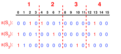
As illustrated in Figure 1, the idea of one permutation hashing is very simple. We view sets as 0/1 vectors in D𝐷D dimensions so that we can treat a collection of sets as a binary data matrix in D𝐷D dimensions. After we permute the columns (features) of the data matrix, we divide the columns evenly into k𝑘k parts (bins) and we simply take, for each data vector, the smallest nonzero element in each bin.
Refer to caption
Figure 1: Fixed-length hashing scheme. Consider S1,S2,S3Ω={0,1,,15}subscript𝑆1subscript𝑆2subscript𝑆3Ω0115S_{1},S_{2},S_{3}\subseteq\Omega=\{0,1,...,15\} (i.e., D=16𝐷16D=16). We apply one permutation π𝜋\pi on the three sets and present π(S1)𝜋subscript𝑆1\pi(S_{1}), π(S2)𝜋subscript𝑆2\pi(S_{2}), and π(S3)𝜋subscript𝑆3\pi(S_{3}) as binary (0/1) vectors, where π(S1)={2,4,7,13}𝜋subscript𝑆124713\pi(S_{1})=\{2,4,7,13\}, π(S2)={0,6,13}𝜋subscript𝑆20613\pi(S_{2})=\{0,6,13\}, and π(S3)={0,1,10,12}𝜋subscript𝑆3011012\pi(S_{3})=\{0,1,10,12\}. We divide the space ΩΩ\Omega evenly into k=4𝑘4k=4 bins, select the smallest nonzero in each bin, and re-index the selected elements as three samples: [2, 0,, 1]2 01[2,\ 0,\ *,\ 1], [0, 2,, 1]021[0,\ 2,\ *,\ 1], and [0,, 2, 0]02 0[0,\ *,\ 2,\ 0]. For now, we use ‘*’ for empty bins, which occur rarely unless the number of nonzeros is small compared to k𝑘k.

In the example in Figure 1 (which concerns 3 sets), the sample selected from π(S1)𝜋subscript𝑆1\pi(S_{1}) is [2,4,,13]2413[2,4,*,13], where we use ’*’ to denote an empty bin, for the time being. Since only want to compare elements with the same bin number (so that we can obtain an inner product), we can actually re-index the elements of each bin to use the smallest possible representations. For example, for π(S1)𝜋subscript𝑆1\pi(S_{1}), after re-indexing, the sample [2,4,,13]2413[2,4,*,13] becomes [24×0,44×1,,134×3]=[2,0,,1]2404411343201[2-4\times 0,4-4\times 1,*,13-4\times 3]=[2,0,*,1]. Similarly, for π(S2)𝜋subscript𝑆2\pi(S_{2}), the original sample [0,6,,13]0613[0,6,*,13] becomes [0,64×1,,134×3]=[0,2,,1]06411343021[0,6-4\times 1,*,13-4\times 3]=[0,2,*,1], etc.

Note that, when there are no empty bins, similarity estimation is equivalent to computing an inner product, which is crucial for taking advantage of the modern linear learning algorithms [13, 19, 7, 11]. We will show that empty bins occur rarely unless the total number of nonzeros for some set is small compared to k𝑘k, and we will present strategies on how to deal with empty bins should they occur.

1.5 Summary of the Advantages of One Permutation Hashing

  • Reducing k𝑘k (e.g., 500) permutations to just one permutation (or a few) is much more computationally efficient. From the perspective of energy consumption, this scheme is highly desirable, especially considering that minwise hashing is deployed in the search industry.

  • While it is true that the preprocessing can be parallelized, it comes at the cost of additional hardware and software implementation.

  • In the testing phase, if a new data point (e.g., a new document or a new image) has to be first processed with k𝑘k permutations, then the testing performance may not meet the demand in for example user-facing applications such as search or interactive visual analytics.

  • It should be much easier to implement the one permutation hashing than the original k𝑘k-permutation scheme, from the perspective of random number generation. For example, if a dataset has one billion features (D=109𝐷superscript109D=10^{9}), we can simply generate a “permutation vector” of length D=109𝐷superscript109D=10^{9}, the memory cost of which (i.e., 4GB) is not significant. On the other hand, it would not be realistic to store a “permutation matrix” of size D×k𝐷𝑘D\times k if D=109𝐷superscript109D=10^{9} and k=500𝑘500k=500; instead, one usually has to resort to approximations such as using universal hashing [5] to approximate permutations. Universal hashing often works well in practice although theoretically there are always worst cases. Of course, when D=264𝐷superscript264D=2^{64}, we have to use universal hashing, but it is always much easier to generate just one permutation.

  • One permutation hashing is a better matrix sparsification scheme than the original k𝑘k-permutation. In terms of the original binary data matrix, the one permutation scheme simply makes many nonzero entries be zero, without further “damaging” the original data matrix. With the original k𝑘k-permutation scheme, we store, for each permutation and each row, only the first nonzero and make all the other nonzero entries be zero; and then we have to concatenate k𝑘k such data matrices. This will significantly change the structure of the original data matrix. As a consequence, we expect that our one permutation scheme will produce at least the same or even more accurate results, as later verified by experiments.

1.6 Related Work

One of the authors worked on another “one permutation” scheme named Conditional Random Sampling (CRS) [14, 15] since 2005. Basically, CRS works by continuously taking the first k𝑘k nonzeros after applying one permutation on the data, then it uses a simple “trick” to construct a random sample for each pair with the effective sample size determined at the estimation stage. By taking the nonzeros continuously, however, the samples are no longer “aligned” and hence we can not write the estimator as an inner product in a unified fashion. In comparison, our new one permutation scheme works by first breaking the columns evenly into k𝑘k bins and then taking the first nonzero in each bin, so that the hashed data can be nicely aligned.

Interestingly, in the original “minwise hashing” paper [4] (we use quotes because the scheme was not called “minwise hashing” at that time), only one permutation was used and a sample was the first k𝑘k nonzeros after the permutation. After the authors of [4] realized that the estimators could not be written as an inner product and hence the scheme was not suitable for many applications such as sublinear time near neighbor search using hash tables, they quickly moved to the k𝑘k-permutation minwise hashing scheme [3]. In the context of large-scale linear learning, the importance of having estimators which are inner products should become more obvious after [18] introduced the idea of using (b𝑏b-bit) minwise hashing for linear learning.

We are also inspired by the work on “very sparse random projections” [16]. The regular random projection method also has the expensive preprocessing cost as it needs k𝑘k projections. The work of [16] showed that one can substantially reduce the preprocessing cost by using an extremely sparse projection matrix. The preprocessing cost of “very sparse random projections” can be as small as merely doing one projection.111See http://www.stanford.edu/group/mmds/slides2012/s-pli.pdf for the experimental results on clustering/classification/regression using very sparse random projections [16].

Figure 1 presents the “fixed-length” scheme, while in Sec. 7 we will also develop a “variable-length” scheme. Two schemes are more or less equivalent, although we believe the fixed-length scheme is more convenient to implement (and it is slightly more accurate). The variable-length hashing scheme is to some extent related to the Count-Min (CM) sketch [6] and the Vowpal Wabbit (VW) [20, 24] hashing algorithms.

2 Applications of Minwise Hashing on Efficient Search and Learning

In this section, we will briefly review two important applications of the original (k𝑘k-permutation) minwise hashing: (i) sublinear time near neighbor search [21], and (ii) large-scale linear learning [18].

2.1 Sublinear Time Near Neighbor Search

The task of near neighbor search is to identify a set of data points which are “most similar” to a query data point. Efficient algorithms for near neighbor search have numerous applications in the context of search, databases, machine learning, recommending systems, computer vision, etc. It has been an active research topic since the early days of modern computing (e.g, [9]).

In current practice, methods for approximate near neighbor search often fall into the general framework of Locality Sensitive Hashing (LSH) [12, 1]. The performance of LSH solely depends on its underlying implementation. The idea in [21] is to directly use the bits generated by (b𝑏b-bit) minwise hashing to construct hash tables, which allow us to search near neighbors in sublinear time (i.e., no need to scan all data points).

Specifically, we hash the data points using k𝑘k random permutations and store each hash value using b𝑏b bits (e.g., b4𝑏4b\leq 4). For each data point, we concatenate the resultant B=b×k𝐵𝑏𝑘B=b\times k bits as a signature. The size of the space is 2B=2b×ksuperscript2𝐵superscript2𝑏𝑘2^{B}=2^{b\times k}, which is not too large for small b𝑏b and k𝑘k (e.g., bk=16𝑏𝑘16bk=16). This way, we create a table of 2Bsuperscript2𝐵2^{B} buckets, numbered from 0 to 2B1superscript2𝐵12^{B}-1; and each bucket stores the pointers of the data points whose signatures match the bucket number. In the testing phrase, we apply the same k𝑘k permutations to a query data point to generate a bk𝑏𝑘bk-bit signature and only search data points in the corresponding bucket. Since using only one hash table will likely miss many true near neighbors, as a remedy, we generate (using independent random permutations) L𝐿L hash tables. The query result is the union of the data points retrieved in L𝐿L tables.

Refer to caption      Refer to caption

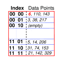
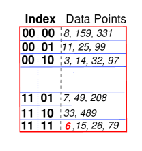
Figure 2: An example of hash tables, with b=2𝑏2b=2, k=2𝑘2k=2, and L=2𝐿2L=2.

Figure 2 provides an example with b=2𝑏2b=2 bits, k=2𝑘2k=2 permutations, and L=2𝐿2L=2 tables. The size of each hash table is 24superscript242^{4}. Given n𝑛n data points, we apply k=2𝑘2k=2 permutations and store b=2𝑏2b=2 bits of each hashed value to generate n𝑛n (4-bit) signatures L𝐿L times. Consider data point 6. For Table 1 (left panel of Figure 2), the lowest b𝑏b-bits of its two hashed values are 00 and 00 and thus its signature is 0000 in binary; hence we place a pointer to data point 6 in bucket number 0. For Table 2 (right panel of Figure 2), we apply another k=2𝑘2k=2 permutations. This time, the signature of data point 6 becomes 1111 in binary and hence we place it in the last bucket. Suppose in the testing phrase, the two (4-bit) signatures of a new data point are 0000 and 1111, respectively. We then only search for the near neighbors in the set {6,15,26,79,110,143}6152679110143\{6,15,26,79,110,143\}, which is much smaller than the set of n𝑛n data points.

The experiments in [21] confirmed that this very simple strategy performed well.

2.2 Large-Scale Linear Learning

The recent development of highly efficient linear learning algorithms (such as linear SVM and logistic regression) is a major breakthrough in machine learning. Popular software packages include SVMperfperf{}^{\text{perf}} [13], Pegasos [19], Bottou’s SGD SVM [2], and LIBLINEAR [7].

Given a dataset {(𝐱i,yi)}i=1nsuperscriptsubscriptsubscript𝐱𝑖subscript𝑦𝑖𝑖1𝑛\{(\mathbf{x}_{i},y_{i})\}_{i=1}^{n}, 𝐱iDsubscript𝐱𝑖superscript𝐷\mathbf{x}_{i}\in\mathbb{R}^{D}, yi{1,1}subscript𝑦𝑖11y_{i}\in\{-1,1\}, the L2subscript𝐿2L_{2}-regularized logistic regression solves the following optimization problem:

min𝐰12𝐰𝐓𝐰+Ci=1nlog(1+eyi𝐰𝐓𝐱𝐢),subscript𝐰12superscript𝐰𝐓𝐰𝐶superscriptsubscript𝑖1𝑛1superscript𝑒subscript𝑦𝑖superscript𝐰𝐓subscript𝐱𝐢\displaystyle\min_{\mathbf{w}}\ \ \frac{1}{2}\mathbf{w^{T}w}+C\sum_{i=1}^{n}\log\left(1+e^{-y_{i}\mathbf{w^{T}x_{i}}}\right), (5)

where C>0𝐶0C>0 is the regularization parameter. The L2subscript𝐿2L_{2}-regularized linear SVM solves a similar problem:

min𝐰12𝐰𝐓𝐰+Ci=1nmax{1yi𝐰𝐓𝐱𝐢, 0},subscript𝐰12superscript𝐰𝐓𝐰𝐶superscriptsubscript𝑖1𝑛1subscript𝑦𝑖superscript𝐰𝐓subscript𝐱𝐢 0\displaystyle\min_{\mathbf{w}}\ \ \frac{1}{2}\mathbf{w^{T}w}+C\sum_{i=1}^{n}\max\left\{1-y_{i}\mathbf{w^{T}x_{i}},\ 0\right\}, (6)

In their approach [18], they apply k𝑘k random permutations on each (binary) feature vector 𝐱isubscript𝐱𝑖\mathbf{x}_{i} and store the lowest b𝑏b bits of each hashed value, to obtain a new dataset which can be stored using merely nbk𝑛𝑏𝑘nbk bits. At run-time, each new data point has to be expanded into a 2b×ksuperscript2𝑏𝑘2^{b}\times k-length vector with exactly k𝑘k 1’s.

To illustrate this simple procedure, [18] provided a toy example with k=3𝑘3k=3 permutations. Suppose for one data vector, the hashed values are {12013, 25964, 20191}120132596420191\{12013,\ 25964,\ 20191\}, whose binary digits are respectively
{010111011101101, 110010101101100,100111011011111}010111011101101110010101101100100111011011111\{010111011101101,\ 110010101101100,100111011011111\}. Using b=2𝑏2b=2 bits, the binary digits are stored as {01,00,11}010011\{01,00,11\} (which corresponds to {1,0,3}103\{1,0,3\} in decimals). At run-time, the (b𝑏b-bit) hashed data are expanded into a vector of length 2bk=12superscript2𝑏𝑘122^{b}k=12, to be {0,0,1,0, 0,0,0,1, 1,0,0,0}0010 00011000\{0,0,1,0,\ \ 0,0,0,1,\ \ 1,0,0,0\}, which will be the new feature vector fed to a solver such as LIBLINEAR. The procedure for this feature vector is summarized as follows:

Original hashed values (k=3):120132596420191Original binary representations:010111011101101110010101101100100111011011111Lowest b=2 binary digits:010011Expanded 2b=4 binary digits :001000011000New feature vector fed to a solver:[0,0,1,0,0,0,0,1,1,0,0,0]×1k:Original hashed values 𝑘3absent120132596420191:Original binary representationsabsent010111011101101110010101101100100111011011111:Lowest b=2 binary digitsabsent010011:Expanded 2b=4 binary digits absent001000011000:New feature vector fed to a solverabsentmissing-subexpression0010000110001𝑘missing-subexpression\displaystyle\begin{array}[]{lrrr}\text{Original hashed values }(k=3):&12013&25964&20191\\ \text{Original binary representations}:&010111011101101&110010101101100&100111011011111\\ \text{Lowest $b=2$ binary digits}:&01&00&11\\ \text{Expanded $2^{b}=4$ binary digits }:&0010&0001&1000\\ \text{New feature vector fed to a solver}:&&[0,0,1,0,0,0,0,1,1,0,0,0]\times\frac{1}{\sqrt{k}}\end{array} (12)

The same procedure (with the same k=3𝑘3k=3 permutations) is then applied to all n𝑛n feature vectors. Very interestingly, we notice that the all-zero vector (0000 in this example) is never used when expanding the data. In our one permutation hashing scheme, we will actually take advantage of the all-zero vector to conveniently encode empty bins, a strategy which we will later refer to as the “zero coding” strategy.

The experiments in [18] confirmed that this simple procedure performed well.

Clearly, in both applications (near neighbor search and linear learning), the hashed data have to be “aligned” in that only the hashed data generated from the same permutation are compared with each other. With our one permutation scheme as presented in Figure 1, the hashed data are indeed aligned according to the bin numbers. The only caveat is that we need a practical strategy to deal with empty bins, although they occur rarely unless the number of nonzeros in one data vector is small compared to k𝑘k, the number of bins.

3 Theoretical Analysis of the Fixed-Length One Permutation Scheme

While the one permutation hashing scheme, as demonstrated in Figure 1, is intuitive, we present in this section some interesting probability analysis to provide a rigorous theoretical foundation for this method. Without loss of generality, we consider two sets S1subscript𝑆1S_{1} and S2subscript𝑆2S_{2}. We first introduce two definitions, for the number of “jointly empty bins” and the number of “matched bins,” respectively:

Nemp=j=1kIemp,j,Nmat=j=1kImat,jformulae-sequencesubscript𝑁𝑒𝑚𝑝superscriptsubscript𝑗1𝑘subscript𝐼𝑒𝑚𝑝𝑗subscript𝑁𝑚𝑎𝑡superscriptsubscript𝑗1𝑘subscript𝐼𝑚𝑎𝑡𝑗\displaystyle N_{emp}=\sum_{j=1}^{k}I_{emp,j},\hskip 43.36243ptN_{mat}=\sum_{j=1}^{k}I_{mat,j} (13)

where Iemp,jsubscript𝐼𝑒𝑚𝑝𝑗I_{emp,j} and Imat,jsubscript𝐼𝑚𝑎𝑡𝑗I_{mat,j} are defined for the j𝑗j-th bin, as

Iemp,j={1if both π(S1) and π(S2) are empty in the j-th bin0otherwisesubscript𝐼𝑒𝑚𝑝𝑗cases1if both 𝜋subscript𝑆1 and 𝜋subscript𝑆2 are empty in the 𝑗-th bin0otherwise\displaystyle I_{emp,j}=\left\{\begin{array}[]{ll}1&\text{if both }\pi(S_{1})\text{ and }\pi(S_{2})\text{ are empty in the }j\text{-th bin}\\ 0&\text{otherwise}\end{array}\right. (16)
Imat,j={1if both π(S1) and π(S1) are not empty and the smallest element of π(S1) matches the smallest element of π(S2),in the j-th bin0otherwisesubscript𝐼𝑚𝑎𝑡𝑗cases1if both 𝜋subscript𝑆1 and 𝜋subscript𝑆1 are not empty and the smallest element of 𝜋subscript𝑆1missing-subexpression matches the smallest element of 𝜋subscript𝑆2in the 𝑗-th bin0otherwise\displaystyle I_{mat,j}=\left\{\begin{array}[]{ll}1&\text{if both }\pi(S_{1})\text{ and }\pi(S_{1})\text{ are not empty and the smallest element of }\pi(S_{1})\\ &\text{ matches the smallest element of }\pi(S_{2}),\hskip 3.61371pt\text{in the }j\text{-th bin}\\ 0&\text{otherwise}\end{array}\right. (20)

Later we will also use Iemp,j(1)superscriptsubscript𝐼𝑒𝑚𝑝𝑗1I_{emp,j}^{(1)} (or Iemp,j(2)superscriptsubscript𝐼𝑒𝑚𝑝𝑗2I_{emp,j}^{(2)}) to indicate whether π(S1)𝜋subscript𝑆1\pi(S_{1}) (or π(S2)𝜋subscript𝑆2\pi(S_{2})) is empty in the j𝑗j-th bin.

3.1 Expectation, Variance, and Distribution of the Number of Jointly Empty Bins

Recall the notation: f1=|S1|,f2=|S2|,a=|S1S2|formulae-sequencesubscript𝑓1subscript𝑆1formulae-sequencesubscript𝑓2subscript𝑆2𝑎subscript𝑆1subscript𝑆2f_{1}=|S_{1}|,\ f_{2}=|S_{2}|,\ a=|S_{1}\cap S_{2}|. We also use f=|S1S2|=f1+f2a𝑓subscript𝑆1subscript𝑆2subscript𝑓1subscript𝑓2𝑎f=|S_{1}\cup S_{2}|=f_{1}+f_{2}-a.

Lemma 1

Assume D(11k)f=f1+f2a𝐷11𝑘𝑓subscript𝑓1subscript𝑓2𝑎D\left(1-\frac{1}{k}\right)\geq f=f_{1}+f_{2}-a,

E(Nemp)k=𝐸subscript𝑁𝑒𝑚𝑝𝑘absent\displaystyle\frac{E\left(N_{emp}\right)}{k}= j=0f1D(11k)jDj(11k)fsuperscriptsubscriptproduct𝑗0𝑓1𝐷11𝑘𝑗𝐷𝑗superscript11𝑘𝑓\displaystyle\prod_{j=0}^{f-1}\frac{D\left(1-\frac{1}{k}\right)-j}{D-j}\leq\left(1-\frac{1}{k}\right)^{f} (21)

Assume D(12k)f=f1+f2a𝐷12𝑘𝑓subscript𝑓1subscript𝑓2𝑎D\left(1-\frac{2}{k}\right)\geq f=f_{1}+f_{2}-a,

Var(Nemp)k2=𝑉𝑎𝑟subscript𝑁𝑒𝑚𝑝superscript𝑘2absent\displaystyle\frac{Var\left(N_{emp}\right)}{k^{2}}= 1k(E(Nemp)k)(1E(Nemp)k)1𝑘𝐸subscript𝑁𝑒𝑚𝑝𝑘1𝐸subscript𝑁𝑒𝑚𝑝𝑘\displaystyle\frac{1}{k}\left(\frac{E(N_{emp})}{k}\right)\left(1-\frac{E(N_{emp})}{k}\right) (22)
(11k)((j=0f1D(11k)jDj)2j=0f1D(12k)jDj)11𝑘superscriptsuperscriptsubscriptproduct𝑗0𝑓1𝐷11𝑘𝑗𝐷𝑗2superscriptsubscriptproduct𝑗0𝑓1𝐷12𝑘𝑗𝐷𝑗\displaystyle-\left(1-\frac{1}{k}\right)\left(\left(\prod_{j=0}^{f-1}\frac{D\left(1-\frac{1}{k}\right)-j}{D-j}\right)^{2}-\prod_{j=0}^{f-1}\frac{D\left(1-\frac{2}{k}\right)-j}{D-j}\right)
<\displaystyle< 1k(E(Nemp)k)(1E(Nemp)k)1𝑘𝐸subscript𝑁𝑒𝑚𝑝𝑘1𝐸subscript𝑁𝑒𝑚𝑝𝑘\displaystyle\frac{1}{k}\left(\frac{E(N_{emp})}{k}\right)\left(1-\frac{E(N_{emp})}{k}\right) (23)

Proof: See Appendix A. \Box

The inequality (23) says that the variance of Nempksubscript𝑁𝑒𝑚𝑝𝑘\frac{N_{emp}}{k} is smaller than its “binomial analog.”

In practical scenarios, the data are often sparse, i.e., f=f1+f2aD𝑓subscript𝑓1subscript𝑓2𝑎much-less-than𝐷f=f_{1}+f_{2}-a\ll D. In this case, Lemma 2 illustrates that in (21) the upper bound (11k)fsuperscript11𝑘𝑓\left(1-\frac{1}{k}\right)^{f} is a good approximation to the true value of E(Nemp)k𝐸subscript𝑁𝑒𝑚𝑝𝑘\frac{E\left(N_{emp}\right)}{k}. Since (11k)fef/ksuperscript11𝑘𝑓superscript𝑒𝑓𝑘\left(1-\frac{1}{k}\right)^{f}\approx e^{-f/k}, we know that the chance of empty bins is small when fkmuch-greater-than𝑓𝑘f\gg k. For example, if f/k=5𝑓𝑘5f/k=5 then (11k)f0.0067superscript11𝑘𝑓0.0067\left(1-\frac{1}{k}\right)^{f}\approx 0.0067; if f/k=1𝑓𝑘1f/k=1, then (11k)f0.3679superscript11𝑘𝑓0.3679\left(1-\frac{1}{k}\right)^{f}\approx 0.3679. For practical applications, we would expect that fkmuch-greater-than𝑓𝑘f\gg k (for most data pairs), otherwise hashing probably would not be too useful anyway. This is why we do not expect empty bins will significantly impact (if at all) the performance in practical settings.

Lemma 2

Assume D(11k)f=f1+f2a𝐷11𝑘𝑓subscript𝑓1subscript𝑓2𝑎D\left(1-\frac{1}{k}\right)\geq f=f_{1}+f_{2}-a.

E(Nemp)k=𝐸subscript𝑁𝑒𝑚𝑝𝑘absent\displaystyle\frac{E\left(N_{emp}\right)}{k}= (11k)fexp(DlogD+1Df+1+f(112(Df+1))k1+)superscript11𝑘𝑓𝐷𝐷1𝐷𝑓1𝑓112𝐷𝑓1𝑘1\displaystyle\left(1-\frac{1}{k}\right)^{f}\exp\left(\frac{-D\log\frac{D+1}{D-f+1}+f\left(1-\frac{1}{2(D-f+1)}\right)}{k-1}+...\right) (24)

Under the reasonable assumption that the data are sparse, i.e., f1+f2a=fDsubscript𝑓1subscript𝑓2𝑎𝑓much-less-than𝐷f_{1}+f_{2}-a=f\ll D, we obtain

E(Nemp)k=𝐸subscript𝑁𝑒𝑚𝑝𝑘absent\displaystyle\frac{E\left(N_{emp}\right)}{k}= (11k)f(1O(f2kD))superscript11𝑘𝑓1𝑂superscript𝑓2𝑘𝐷\displaystyle\left(1-\frac{1}{k}\right)^{f}\left(1-O\left(\frac{f^{2}}{kD}\right)\right) (25)
Var(Nemp)k2=𝑉𝑎𝑟subscript𝑁𝑒𝑚𝑝superscript𝑘2absent\displaystyle\frac{Var\left(N_{emp}\right)}{k^{2}}= 1k(11k)f(1(11k)f)1𝑘superscript11𝑘𝑓1superscript11𝑘𝑓\displaystyle\frac{1}{k}\left(1-\frac{1}{k}\right)^{f}\left(1-\left(1-\frac{1}{k}\right)^{f}\right) (26)
(11k)f+1((11k)f(11k1)f)+O(f2kD)superscript11𝑘𝑓1superscript11𝑘𝑓superscript11𝑘1𝑓𝑂superscript𝑓2𝑘𝐷\displaystyle-\left(1-\frac{1}{k}\right)^{f+1}\left(\left(1-\frac{1}{k}\right)^{f}-\left(1-\frac{1}{k-1}\right)^{f}\right)+O\left(\frac{f^{2}}{kD}\right)

Proof: See Appendix B. \Box

In addition to its mean and variance, we can also write down the distribution of Nempsubscript𝑁𝑒𝑚𝑝N_{emp}.

Lemma 3
𝐏𝐫(Nemp=j)=s=0kj(1)sk!j!s!(kjs)!t=0f1D(1j+sk)tDt𝐏𝐫subscript𝑁𝑒𝑚𝑝𝑗superscriptsubscript𝑠0𝑘𝑗superscript1𝑠𝑘𝑗𝑠𝑘𝑗𝑠superscriptsubscriptproduct𝑡0𝑓1𝐷1𝑗𝑠𝑘𝑡𝐷𝑡\displaystyle\mathbf{Pr}\left(N_{emp}=j\right)=\sum_{s=0}^{k-j}(-1)^{s}\frac{k!}{j!s!(k-j-s)!}\prod_{t=0}^{f-1}\frac{D\left(1-\frac{j+s}{k}\right)-t}{D-t} (27)

Proof: See Appendix C. \Box

Because E(Nemp)=j=0k1j𝐏𝐫(Nemp=j)𝐸subscript𝑁𝑒𝑚𝑝superscriptsubscript𝑗0𝑘1𝑗𝐏𝐫subscript𝑁𝑒𝑚𝑝𝑗E\left(N_{emp}\right)=\sum_{j=0}^{k-1}j\mathbf{Pr}\left(N_{emp}=j\right), this yields an interesting combinatorial identity:

kj=0f1D(11k)jDj=j=0k1js=0kj(1)sk!j!s!(kjs)!t=0f1D(1j+sk)tDt𝑘superscriptsubscriptproduct𝑗0𝑓1𝐷11𝑘𝑗𝐷𝑗superscriptsubscript𝑗0𝑘1𝑗superscriptsubscript𝑠0𝑘𝑗superscript1𝑠𝑘𝑗𝑠𝑘𝑗𝑠superscriptsubscriptproduct𝑡0𝑓1𝐷1𝑗𝑠𝑘𝑡𝐷𝑡\displaystyle k\prod_{j=0}^{f-1}\frac{D\left(1-\frac{1}{k}\right)-j}{D-j}=\sum_{j=0}^{k-1}j\sum_{s=0}^{k-j}(-1)^{s}\frac{k!}{j!s!(k-j-s)!}\prod_{t=0}^{f-1}\frac{D\left(1-\frac{j+s}{k}\right)-t}{D-t} (28)

3.2 Expectation and Variance of the Number of Matched Bins

Lemma 4

Assume D(11k)f=f1+f2a𝐷11𝑘𝑓subscript𝑓1subscript𝑓2𝑎D\left(1-\frac{1}{k}\right)\geq f=f_{1}+f_{2}-a.

E(Nmat)k=R(1E(Nemp)k)=R(1j=0f1D(11k)jDj)𝐸subscript𝑁𝑚𝑎𝑡𝑘𝑅1𝐸subscript𝑁𝑒𝑚𝑝𝑘𝑅1superscriptsubscriptproduct𝑗0𝑓1𝐷11𝑘𝑗𝐷𝑗\displaystyle\frac{E\left(N_{mat}\right)}{k}=R\left(1-\frac{E\left(N_{emp}\right)}{k}\right)=R\left(1-\prod_{j=0}^{f-1}\frac{D\left(1-\frac{1}{k}\right)-j}{D-j}\right) (29)

Assume D(12k)f=f1+f2a𝐷12𝑘𝑓subscript𝑓1subscript𝑓2𝑎D\left(1-\frac{2}{k}\right)\geq f=f_{1}+f_{2}-a.

Var(Nmat)k2=𝑉𝑎𝑟subscript𝑁𝑚𝑎𝑡superscript𝑘2absent\displaystyle\frac{Var(N_{mat})}{k^{2}}= 1k(E(Nmat)k)(1E(Nmat)k)1𝑘𝐸subscript𝑁𝑚𝑎𝑡𝑘1𝐸subscript𝑁𝑚𝑎𝑡𝑘\displaystyle\frac{1}{k}\left(\frac{E(N_{mat})}{k}\right)\left(1-\frac{E(N_{mat})}{k}\right) (30)
+(11k)Ra1f1(12j=0f1D(11k)jDj+j=0f1D(12k)jDj)11𝑘𝑅𝑎1𝑓112superscriptsubscriptproduct𝑗0𝑓1𝐷11𝑘𝑗𝐷𝑗superscriptsubscriptproduct𝑗0𝑓1𝐷12𝑘𝑗𝐷𝑗\displaystyle+\left(1-\frac{1}{k}\right)R\frac{a-1}{f-1}\left(1-2\prod_{j=0}^{f-1}\frac{D\left(1-\frac{1}{k}\right)-j}{D-j}+\prod_{j=0}^{f-1}\frac{D\left(1-\frac{2}{k}\right)-j}{D-j}\right)
(11k)R2(1j=0f1D(11k)jDj)211𝑘superscript𝑅2superscript1superscriptsubscriptproduct𝑗0𝑓1𝐷11𝑘𝑗𝐷𝑗2\displaystyle-\left(1-\frac{1}{k}\right)R^{2}\left(1-\prod_{j=0}^{f-1}\frac{D\left(1-\frac{1}{k}\right)-j}{D-j}\right)^{2}
<\displaystyle< 1k(E(Nmat)k)(1E(Nmat)k)1𝑘𝐸subscript𝑁𝑚𝑎𝑡𝑘1𝐸subscript𝑁𝑚𝑎𝑡𝑘\displaystyle\frac{1}{k}\left(\frac{E(N_{mat})}{k}\right)\left(1-\frac{E(N_{mat})}{k}\right) (31)

Proof: See Appendix D. \Box

3.3 Covariance of Nmatsubscript𝑁𝑚𝑎𝑡N_{mat} and Nempsubscript𝑁𝑒𝑚𝑝N_{emp}

Intuitively, Nmatsubscript𝑁𝑚𝑎𝑡N_{mat} and Nempsubscript𝑁𝑒𝑚𝑝N_{emp} should be negatively correlated, as confirmed by the following Lemma:

Lemma 5

Assume D(12k)f=f1+f2a𝐷12𝑘𝑓subscript𝑓1subscript𝑓2𝑎D\left(1-\frac{2}{k}\right)\geq f=f_{1}+f_{2}-a.

Cov(Nmat,Nemp)k2=𝐶𝑜𝑣subscript𝑁𝑚𝑎𝑡subscript𝑁𝑒𝑚𝑝superscript𝑘2absent\displaystyle\frac{Cov\left(N_{mat},\ N_{emp}\right)}{k^{2}}= R(j=0f1D(11k)jDj)(j=0f1D(11k)jDjj=0f1D(12k)jD(11k)j)𝑅superscriptsubscriptproduct𝑗0𝑓1𝐷11𝑘𝑗𝐷𝑗superscriptsubscriptproduct𝑗0𝑓1𝐷11𝑘𝑗𝐷𝑗superscriptsubscriptproduct𝑗0𝑓1𝐷12𝑘𝑗𝐷11𝑘𝑗\displaystyle R\left(\prod_{j=0}^{f-1}\frac{D\left(1-\frac{1}{k}\right)-j}{D-j}\right)\left(\prod_{j=0}^{f-1}\frac{D\left(1-\frac{1}{k}\right)-j}{D-j}-\prod_{j=0}^{f-1}\frac{D\left(1-\frac{2}{k}\right)-j}{D\left(1-\frac{1}{k}\right)-j}\right)
1kR(1j=0f1D(12k)jD(11k)j)(j=0f1D(11k)jDj)1𝑘𝑅1superscriptsubscriptproduct𝑗0𝑓1𝐷12𝑘𝑗𝐷11𝑘𝑗superscriptsubscriptproduct𝑗0𝑓1𝐷11𝑘𝑗𝐷𝑗\displaystyle-\frac{1}{k}R\left(1-\prod_{j=0}^{f-1}\frac{D\left(1-\frac{2}{k}\right)-j}{D\left(1-\frac{1}{k}\right)-j}\right)\left(\prod_{j=0}^{f-1}\frac{D\left(1-\frac{1}{k}\right)-j}{D-j}\right) (32)

and

Cov(Nmat,Nemp)0𝐶𝑜𝑣subscript𝑁𝑚𝑎𝑡subscript𝑁𝑒𝑚𝑝0\displaystyle Cov\left(N_{mat},\ N_{emp}\right)\leq 0 (33)

Proof: See Appendix E. \Box

3.4 An Unbiased Estimator of R𝑅R and the Variance

Lemma 6 shows the following estimator R^matsubscript^𝑅𝑚𝑎𝑡\hat{R}_{mat} of the resemblance is unbiased:

Lemma 6
R^mat=NmatkNemp,E(R^mat)=Rformulae-sequencesubscript^𝑅𝑚𝑎𝑡subscript𝑁𝑚𝑎𝑡𝑘subscript𝑁𝑒𝑚𝑝𝐸subscript^𝑅𝑚𝑎𝑡𝑅\displaystyle\hat{R}_{mat}=\frac{N_{mat}}{k-N_{emp}},\hskip 14.45377ptE\left(\hat{R}_{mat}\right)=R (34)
Var(R^mat)=R(1R)(E(1kNemp)(1+1f1)1f1)𝑉𝑎𝑟subscript^𝑅𝑚𝑎𝑡𝑅1𝑅𝐸1𝑘subscript𝑁𝑒𝑚𝑝11𝑓11𝑓1\displaystyle Var\left(\hat{R}_{mat}\right)=R(1-R)\left(E\left(\frac{1}{k-N_{emp}}\right)\left(1+\frac{1}{f-1}\right)-\frac{1}{f-1}\right) (35)
E(1kNemp)=j=0k1𝐏𝐫(Nemp=j)kj1kE(Nemp)𝐸1𝑘subscript𝑁𝑒𝑚𝑝superscriptsubscript𝑗0𝑘1𝐏𝐫subscript𝑁𝑒𝑚𝑝𝑗𝑘𝑗1𝑘𝐸subscript𝑁𝑒𝑚𝑝\displaystyle E\left(\frac{1}{k-N_{emp}}\right)=\sum_{j=0}^{k-1}\frac{\mathbf{Pr}\left(N_{emp}=j\right)}{k-j}\geq\frac{1}{k-E(N_{emp})} (36)

Proof: See Appendix F. The right-hand side of the inequality (36) is actually a very good approximation (see Figure 8). The exact expression for 𝐏𝐫(Nemp=j)𝐏𝐫subscriptNempj\mathbf{Pr}\left(N_{emp}=j\right) is already derived in Lemma 3. \Box

The fact that E(R^mat)=R𝐸subscript^𝑅𝑚𝑎𝑡𝑅E\left(\hat{R}_{mat}\right)=R may seem surprising as in general ratio estimators are not unbiased. Note that kNemp>0𝑘subscript𝑁𝑒𝑚𝑝0k-N_{emp}>0 always because we assume the original data vectors are not completely empty (all-zero).

As expected, when kf=f1+f2amuch-less-than𝑘𝑓subscript𝑓1subscript𝑓2𝑎k\ll f=f_{1}+f_{2}-a, Nempsubscript𝑁𝑒𝑚𝑝N_{emp} is essentially zero and hence Var(R^mat)R(1R)k𝑉𝑎𝑟subscript^𝑅𝑚𝑎𝑡𝑅1𝑅𝑘Var\left(\hat{R}_{mat}\right)\approx\frac{R(1-R)}{k}. In fact, Var(R^mat)𝑉𝑎𝑟subscript^𝑅𝑚𝑎𝑡Var\left(\hat{R}_{mat}\right) is somewhat smaller than R(1R)k𝑅1𝑅𝑘\frac{R(1-R)}{k}, which can be seen from the approximation:

Var(R^mat)R(1R)/kg(f;k)=11(11k)f(1+1f1)kf1𝑉𝑎𝑟subscript^𝑅𝑚𝑎𝑡𝑅1𝑅𝑘𝑔𝑓𝑘11superscript11𝑘𝑓11𝑓1𝑘𝑓1\displaystyle\frac{Var\left(\hat{R}_{mat}\right)}{R(1-R)/k}\approx g(f;k)=\frac{1}{1-\left(1-\frac{1}{k}\right)^{f}}\left(1+\frac{1}{f-1}\right)-\frac{k}{f-1} (37)
Lemma 7
g(f;k)1𝑔𝑓𝑘1\displaystyle\vspace{-0.2in}g(f;k)\leq 1 (38)

Proof: See Appendix G. \Box

It is probably not surprising that our one permutation scheme may (slightly) outperform the original k𝑘k-permutation scheme (at merely 1/k1𝑘1/k of its preprocessing cost), because one permutation hashing can be viewed as a “sample-without-replacement” scheme.

3.5 Experiments for Validating the Theoretical Results

This set of experiments is for validating the theoretical results. The Web crawl dataset (in Table 1) consists of 15 (essentially randomly selected) pairs of word vectors (in D=216𝐷superscript216D=2^{16} dimensions) of a range of similarities and sparsities. For each word vector, the j𝑗j-th element is whether the word appeared in the j𝑗j-th Web page.

Table 1: 15 pairs of English words. For example, “RIGHTS” and “RESERVED” correspond to the two sets of document IDs which contained word “RIGHTS” and word “RESERVED” respectively.
Word 1 Word 2 f1subscript𝑓1f_{1} f2subscript𝑓2f_{2} f=f1+f2a𝑓subscript𝑓1subscript𝑓2𝑎f=f_{1}+f_{2}-a R𝑅R
RIGHTS RESERVED 12234 11272 12526 0.877
OF AND 37339 36289 41572 0.771
THIS HAVE 27695 17522 31647 0.429
ALL MORE 26668 17909 31638 0.409
CONTACT INFORMATION 16836 16339 24974 0.328
MAY ONLY 12067 11006 17953 0.285
CREDIT CARD 2999 2697 4433 0.285
SEARCH WEB 1402 12718 21770 0.229
RESEARCH UNIVERSITY 4353 4241 7017 0.225
FREE USE 12406 11744 19782 0.221
TOP BUSINESS 9151 8284 14992 0.163
BOOK TRAVEL 5153 4608 8542 0.143
TIME JOB 12386 3263 13874 0.128
REVIEW PAPER 3197 1944 4769 0.078
A TEST 39063 2278 2060 0.052

We vary k𝑘k from 23superscript232^{3} to 215superscript2152^{15}. Although k=215𝑘superscript215k=2^{15} is probably way too large in practice, we use it for the purpose of thorough validations. Figures 3 to 8 present the empirical results based on 105superscript10510^{5} repetitions.

3.5.1 E(Nemp)𝐸subscript𝑁𝑒𝑚𝑝E(N_{emp}) and Var(Nemp)𝑉𝑎𝑟subscript𝑁𝑒𝑚𝑝Var(N_{emp})

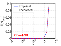
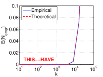
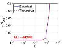
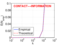
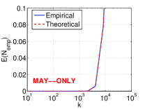
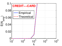
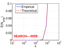
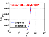
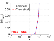
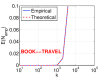
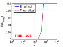
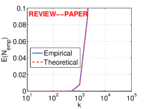
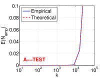
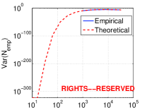
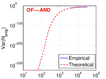
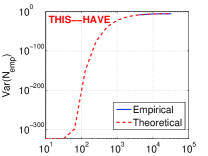
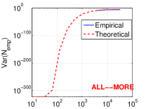
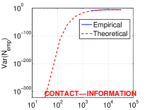
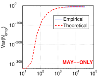
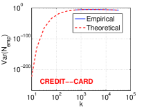
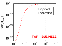
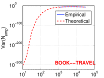
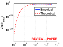
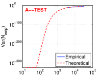
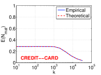
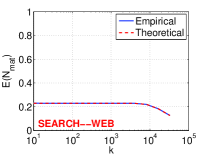
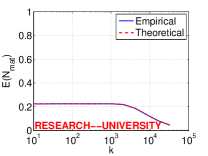
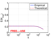
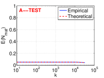
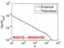
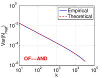
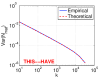
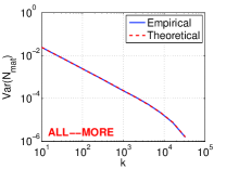
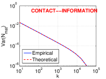
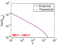
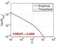
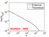
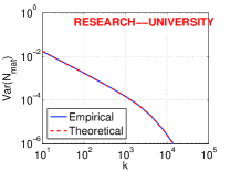
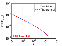
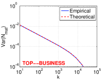
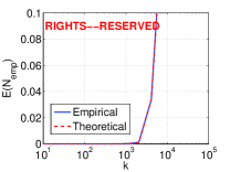
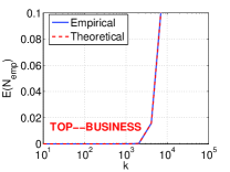
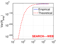
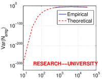
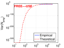
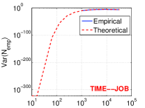
Figure 3 and Figure 4 respectively verify E(Nemp)𝐸subscript𝑁𝑒𝑚𝑝E(N_{emp}) and Var(Nemp)𝑉𝑎𝑟subscript𝑁𝑒𝑚𝑝Var(N_{emp}) as derived in Lemma 1. Clearly, the theoretical curves overlap the empirical curves.

Note that Nempsubscript𝑁𝑒𝑚𝑝N_{emp} is essentially 0 when k𝑘k is not large. Roughly when k/f>1/5𝑘𝑓15k/f>1/5, the number of empty bins becomes noticeable, which is expected because E(Nemp)/k(11k)fef/k𝐸subscript𝑁𝑒𝑚𝑝𝑘superscript11𝑘𝑓superscript𝑒𝑓𝑘E(N_{emp})/k\approx\left(1-\frac{1}{k}\right)^{f}\approx e^{-f/k} and e5=0.0067superscript𝑒50.0067e^{-5}=0.0067. Practically speaking, as we often use minwise hashing to substantially reduce the number of nonzeros in massive datasets, we would expect that usually fkmuch-greater-than𝑓𝑘f\gg k anyway. See Sec. 4 for more discussion about strategies for dealing with empty bins.
Refer to caption Refer to caption Refer to caption Refer to caption Refer to caption Refer to caption Refer to caption Refer to caption Refer to caption Refer to caption Refer to caption Refer to caption Refer to caption Refer to caption Refer to caption

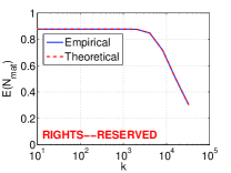
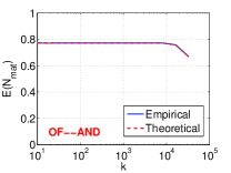
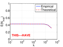
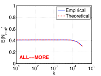
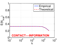
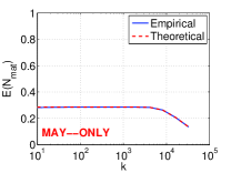
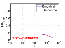
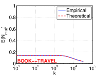
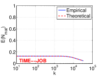
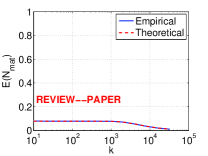
Figure 3: E(Nemp)/k𝐸subscript𝑁𝑒𝑚𝑝𝑘E(N_{emp})/k. The empirical curves essentially overlap the theoretical curves as derived in Lemma 1, i.e., (21). The occurrences of empty bins become noticeable only at relatively large sample size k𝑘k.

Refer to caption Refer to caption Refer to caption Refer to caption Refer to caption Refer to caption Refer to caption Refer to caption Refer to caption Refer to caption Refer to caption Refer to caption Refer to caption Refer to caption Refer to caption

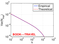
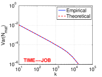
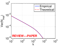
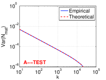
Figure 4: Var(Nemp)/k2𝑉𝑎𝑟subscript𝑁𝑒𝑚𝑝superscript𝑘2Var(N_{emp})/k^{2}. The empirical curves essentially overlap the theoretical curves as derived in Lemma 1, i.e., (22).

3.5.2 E(Nmat)𝐸subscript𝑁𝑚𝑎𝑡E(N_{mat}) and Var(Nmat)𝑉𝑎𝑟subscript𝑁𝑚𝑎𝑡Var(N_{mat})

Figure 5 and Figure 6 respectively verify E(Nmat)𝐸subscript𝑁𝑚𝑎𝑡E(N_{mat}) and Var(Nmat)𝑉𝑎𝑟subscript𝑁𝑚𝑎𝑡Var(N_{mat}) as derived in Lemma 4. Again, the theoretical curves match the empirical ones and the curves start to change shapes at the point where the occurrences of empty bins are more noticeable.

Refer to caption Refer to caption Refer to caption Refer to caption Refer to caption Refer to caption Refer to caption Refer to caption Refer to caption Refer to caption Refer to caption Refer to caption Refer to caption Refer to caption Refer to caption

Figure 5: E(Nmat)/k𝐸subscript𝑁𝑚𝑎𝑡𝑘E(N_{mat})/k. The empirical curves essentially overlap the theoretical curves as derived in Lemma 4, i.e., (29).

Refer to caption Refer to caption Refer to caption Refer to caption Refer to caption Refer to caption Refer to caption Refer to caption Refer to caption Refer to caption Refer to caption Refer to caption Refer to caption Refer to caption Refer to caption

Figure 6: Var(Nmat)/k2𝑉𝑎𝑟subscript𝑁𝑚𝑎𝑡superscript𝑘2Var(N_{mat})/k^{2}. The empirical curves essentially overlap the theoretical curves as derived in Lemma 4, i.e., (30).

3.5.3 Cov(Nemp,Nmat)𝐶𝑜𝑣subscript𝑁𝑒𝑚𝑝subscript𝑁𝑚𝑎𝑡Cov(N_{emp},N_{mat})

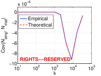
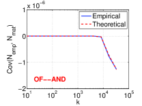
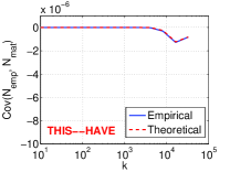
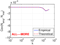
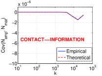
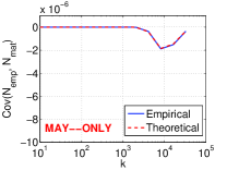
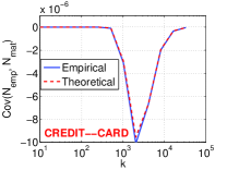
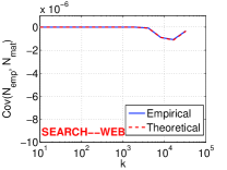
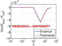
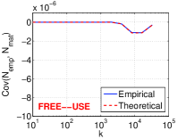
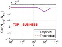
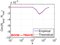
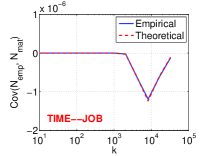
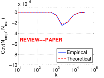
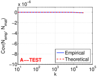
To verify Lemma 5, Figure 7 presents the theoretical and empirical covariances of Nempsubscript𝑁𝑒𝑚𝑝N_{emp} and Nmatsubscript𝑁𝑚𝑎𝑡N_{mat}. Note that Cov(Nemp,Nmat)0𝐶𝑜𝑣subscript𝑁𝑒𝑚𝑝subscript𝑁𝑚𝑎𝑡0Cov\left(N_{emp},\ N_{mat}\right)\leq 0 as shown in Lemma 5.

Refer to caption Refer to caption Refer to caption Refer to caption Refer to caption Refer to caption Refer to caption Refer to caption Refer to caption Refer to caption Refer to caption Refer to caption Refer to caption Refer to caption Refer to caption

Figure 7: Cov(Nemp,Nmat)/k2𝐶𝑜𝑣subscript𝑁𝑒𝑚𝑝subscript𝑁𝑚𝑎𝑡superscript𝑘2Cov(N_{emp},N_{mat})/k^{2}. The empirical curves essentially overlap the theoretical curves as derived in Lemma 5, i.e., (32). The experimental results also confirm that the covariance is non-positive as theoretically shown in Lemma 5.

3.5.4 E(R^mat)𝐸subscript^𝑅𝑚𝑎𝑡E(\hat{R}_{mat}) and Var(R^mat)𝑉𝑎𝑟subscript^𝑅𝑚𝑎𝑡Var(\hat{R}_{mat})

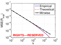
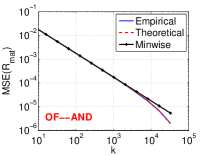
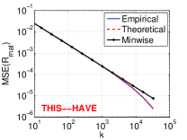
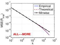
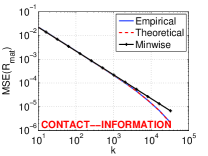
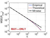
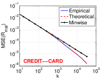
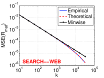
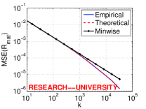
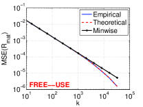
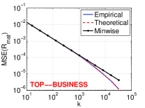
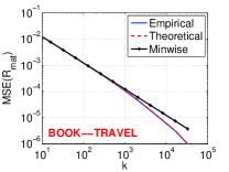
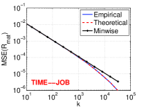
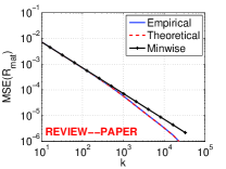
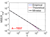
Finally, Figure 8 plots the empirical MSEs (MSE = bias2 + variance) and the theoretical variances (35), where the term E(1kNemp)𝐸1𝑘subscript𝑁𝑒𝑚𝑝E\left(\frac{1}{k-N_{emp}}\right) is approximated by 1kE(Nemp)1𝑘𝐸subscript𝑁𝑒𝑚𝑝\frac{1}{k-E(N_{emp})} as in (36).

The experimental results confirm Lemma 6: (i) the estimator R^matsubscript^𝑅𝑚𝑎𝑡\hat{R}_{mat} is unbiased; (ii) the variance formula (35) and the approximation (36) are accurate; (iii) the variance of R^matsubscript^𝑅𝑚𝑎𝑡\hat{R}_{mat} is somewhat smaller than R(1R)/k𝑅1𝑅𝑘R(1-R)/k, which is the variance of the original k𝑘k-permutation minwise hashing, due to the “sample-without-replacement” effect.

Refer to caption Refer to caption Refer to caption Refer to caption Refer to caption Refer to caption Refer to caption Refer to caption Refer to caption Refer to caption Refer to caption Refer to caption Refer to caption Refer to caption Refer to caption

Figure 8: MSE(R^mat)𝑀𝑆𝐸subscript^𝑅𝑚𝑎𝑡MSE(\hat{R}_{mat}), to verify the theoretical results of Lemma 6. Note that the theoretical variance curves use the approximation (36), for convenience. The experimental results confirm that: (i) the estimator R^matsubscript^𝑅𝑚𝑎𝑡\hat{R}_{mat} is unbiased, (ii) the variance formula (35) and the approximation (36) are accurate; (iii) the variance of R^matsubscript^𝑅𝑚𝑎𝑡\hat{R}_{mat} is somewhat smaller than R(1R)/k𝑅1𝑅𝑘R(1-R)/k, the variance of the original k𝑘k-permutation minwise hashing.

Remark: The empirical results presented in Figures 3 to 8 have clearly validated the theoretical results for our one permutation hashing scheme. Note that we did not add the empirical results of the original k𝑘k-permutation minwise hashing scheme because they would simply overlap the theoretical curves. The fact that the original k𝑘k-permutation scheme provides the unbiased estimate of R𝑅R with variance R(1R)k𝑅1𝑅𝑘\frac{R(1-R)}{k} has been well-validated in prior literature, for example [17].

4 Strategies for Dealing with Empty Bins

In general, we expect that empty bins should not occur often because E(Nemp)/kef/k𝐸subscript𝑁𝑒𝑚𝑝𝑘superscript𝑒𝑓𝑘E(N_{emp})/k\approx e^{-f/k}, which is very close to zero if f/k>5𝑓𝑘5f/k>5. (Recall f=|S1S2|𝑓subscript𝑆1subscript𝑆2f=|S_{1}\cup S_{2}|.) If the goal of using minwise hashing is for data reduction, i.e., reducing the number of nonzeros, then we would expect that fkmuch-greater-than𝑓𝑘f\gg k anyway.

Nevertheless, in applications where we need the estimators to be inner products, we need strategies to deal with empty bins in case they occur. Fortunately, we realize a (in retrospect) simple strategy which can be very nicely integrated with linear learning algorithms and performs very well.

Refer to caption
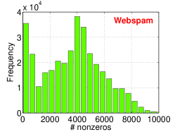
Figure 9: Histogram of the numbers of nonzeros in the webspam dataset (350,000 samples).

Figure 9 plots the histogram of the numbers of nonzeros in the webspam dataset, which has 350,000 samples. The average number of nonzeros is about 4000 which should be much larger than the k𝑘k (e.g., 200 to 500) for the hashing procedure. On the other hand, about 10%percent1010\% (or 2.8%percent2.82.8\%) of the samples have <500absent500<500 (or <200absent200<200) nonzeros. Thus, we must deal with empty bins if we do not want to exclude those data points. For example, if f=k=500𝑓𝑘500f=k=500, then Nempef/k=0.3679subscript𝑁𝑒𝑚𝑝superscript𝑒𝑓𝑘0.3679N_{emp}\approx e^{-f/k}=0.3679, which is not small.

The first (obvious) idea is random coding. That is, we simply replace an empty bin (i.e., “*” as in Figure 1) with a random number. In terms of the original unbiased estimator R^mat=NmatkNempsubscript^𝑅𝑚𝑎𝑡subscript𝑁𝑚𝑎𝑡𝑘subscript𝑁𝑒𝑚𝑝\hat{R}_{mat}=\frac{N_{mat}}{k-N_{emp}}, the random coding scheme will almost not change the numerator Nmatsubscript𝑁𝑚𝑎𝑡N_{mat}. The drawback of random coding is that the denominator will effectively become k𝑘k. Of course, in most practical scenarios, we expect Nemp0subscript𝑁𝑒𝑚𝑝0N_{emp}\approx 0 anyway.

The strategy we recommend for linear learning is zero coding, which is tightly coupled with the strategy of hashed data expansion [18] as reviewed in Sec. 2.2. More details will be elaborated in Sec. 4.2. Basically, we can encode “*” as “zero” in the expanded space, which means Nmatsubscript𝑁𝑚𝑎𝑡N_{mat} will remain the same (after taking the inner product in the expanded space). A very nice property of this strategy is that it is sparsity-preserving. This strategy essentially corresponds to the following modified estimator:

R^mat(0)=NmatkNemp(1)kNemp(2)superscriptsubscript^𝑅𝑚𝑎𝑡0subscript𝑁𝑚𝑎𝑡𝑘superscriptsubscript𝑁𝑒𝑚𝑝1𝑘superscriptsubscript𝑁𝑒𝑚𝑝2\displaystyle\hat{R}_{mat}^{(0)}=\frac{N_{mat}}{\sqrt{k-N_{emp}^{(1)}}\sqrt{k-N_{emp}^{(2)}}} (39)

where Nemp(1)=j=1kIemp,j(1)superscriptsubscript𝑁𝑒𝑚𝑝1superscriptsubscript𝑗1𝑘superscriptsubscript𝐼𝑒𝑚𝑝𝑗1N_{emp}^{(1)}=\sum_{j=1}^{k}I_{emp,j}^{(1)} and Nemp(2)=j=1kIemp,j(2)superscriptsubscript𝑁𝑒𝑚𝑝2superscriptsubscript𝑗1𝑘superscriptsubscript𝐼𝑒𝑚𝑝𝑗2N_{emp}^{(2)}=\sum_{j=1}^{k}I_{emp,j}^{(2)} are the numbers of empty bins in π(S1)𝜋subscript𝑆1\pi(S_{1}) and π(S2)𝜋subscript𝑆2\pi(S_{2}), respectively. This modified estimator actually makes a lot of sense, after some careful thinking.

Basically, since each data vector is processed and coded separately, we actually do not know Nempsubscript𝑁𝑒𝑚𝑝N_{emp} (the number of jointly empty bins) until we see both π(S1)𝜋subscript𝑆1\pi(S_{1}) and π(S2)𝜋subscript𝑆2\pi(S_{2}). In other words, we can not really compute Nempsubscript𝑁𝑒𝑚𝑝N_{emp} if we want to use linear estimators. On the other hand, Nemp(1)superscriptsubscript𝑁𝑒𝑚𝑝1N_{emp}^{(1)} and Nemp(2)superscriptsubscript𝑁𝑒𝑚𝑝2N_{emp}^{(2)} are always available. In fact, the use of kNemp(1)kNemp(2)𝑘superscriptsubscript𝑁𝑒𝑚𝑝1𝑘superscriptsubscript𝑁𝑒𝑚𝑝2\sqrt{k-N_{emp}^{(1)}}\sqrt{k-N_{emp}^{(2)}} in the denominator corresponds to the normalizing step which is usually needed before feeding the data to a solver. This point will probably become more clear in Sec. 4.2.

When Nemp(1)=Nemp(2)=Nempsuperscriptsubscript𝑁𝑒𝑚𝑝1superscriptsubscript𝑁𝑒𝑚𝑝2subscript𝑁𝑒𝑚𝑝N_{emp}^{(1)}=N_{emp}^{(2)}=N_{emp}, (39) is equivalent to the original R^matsubscript^𝑅𝑚𝑎𝑡\hat{R}_{mat}. When two original vectors are very similar (e.g., large R𝑅R), Nemp(1)superscriptsubscript𝑁𝑒𝑚𝑝1N_{emp}^{(1)} and Nemp(2)superscriptsubscript𝑁𝑒𝑚𝑝2N_{emp}^{(2)} will be close to Nempsubscript𝑁𝑒𝑚𝑝N_{emp}. When two sets are highly unbalanced, using (39) will likely overestimate R𝑅R; however, in this case, Nmatsubscript𝑁𝑚𝑎𝑡N_{mat} will be so small that the absolute error will not be large. In any case, we do not expect the existence of empty bins will significantly affect the performance in practical settings.

4.1 The m𝑚m-Permutation Scheme with 1<mk1𝑚much-less-than𝑘1<m\ll k

In case some readers would like to further (significantly) reduce the chance of the occurrences of empty bins, here we shall mention that one does not really have to strictly follow “one permutation,” since one can always conduct m𝑚m permutations with k=k/msuperscript𝑘𝑘𝑚k^{\prime}=k/m and concatenate the hashed data. Once the preprocessing is no longer the bottleneck, it matters less whether we use 1 permutation or (e.g.,) m=3𝑚3m=3 permutations. The chance of having empty bins decreases exponentially with increasing m𝑚m.

4.2 An Example of The “Zero Coding” Strategy for Linear Learning

Sec. 2.2 has already reviewed the data-expansion strategy used by [18] for integrating (b𝑏b-bit) minwise hashing with linear learning. We will adopt a similar strategy with modifications for considering empty bins.

We use a similar example as in Sec. 2.2. Suppose we apply our one permutation hashing scheme and use k=4𝑘4k=4 bins. For the first data vector, the hashed values are [12013, 25964, 20191,]120132596420191[12013,\ 25964,\ 20191,\ *] (i.e., the 4-th bin is empty). Suppose again we use b=2𝑏2b=2 bits. With the “zero coding” strategy, our procedure is summarized as follows:

Original hashed values (k=4):120132596420191Original binary representations:010111011101101110010101101100100111011011111Lowest b=2 binary digits:010011Expanded 2b=4 binary digits :0010000110000000:Original hashed values 𝑘4absent120132596420191:Original binary representationsabsent010111011101101110010101101100100111011011111:Lowest b=2 binary digitsabsent010011:Expanded 2b=4 binary digits absent0010000110000000\displaystyle\begin{array}[]{lrrrr}\text{Original hashed values }(k=4):&12013&25964&20191&*\\ \text{Original binary representations}:&010111011101101&110010101101100&100111011011111&*\\ \text{Lowest $b=2$ binary digits}:&01&00&11&*\\ \text{Expanded $2^{b}=4$ binary digits }:&0010&0001&1000&{\color[rgb]{1,0,0}0000}\\ \end{array} (44)
New feature vector fed to a solver:141×[0,0,1,0,0,0,0,1,1,0,0,0,0,0,0,0]:New feature vector fed to a solver1410010000110000000\displaystyle\text{New feature vector fed to a solver}:\frac{1}{\sqrt{\color[rgb]{1,0,0}4-1}}\times[0,0,1,0,0,0,0,1,1,0,0,0,0,0,0,0]

We apply the same procedure to all feature vectors in the data matrix to generate a new data matrix. The normalization factor 1kNemp(i)1𝑘superscriptsubscript𝑁𝑒𝑚𝑝𝑖\frac{1}{\sqrt{k-N_{emp}^{(i)}}} varies, depending on the number of empty bins in the i𝑖i-th feature vector.

We believe zero coding is an ideal strategy for dealing with empty bins in the context of linear learning as it is very convenient and produces accurate results (as we will show by experiments). If we use the “random coding” strategy (i.e., replacing a “*” by a random number in [0, 2b1]0superscript2𝑏1[0,\ 2^{b}-1]), we need to add artificial nonzeros (in the expanded space) and the normalizing factor is always 1k1𝑘\frac{1}{\sqrt{k}} (i.e., no longer “sparsity-preserving”).

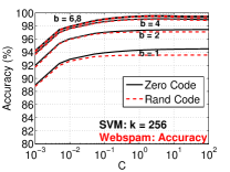
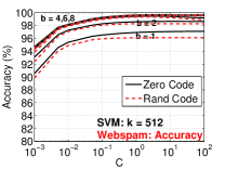
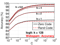
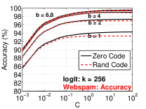
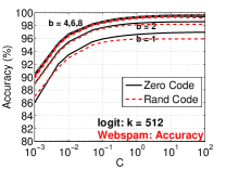
We apply both the zero coding and random coding strategies on the webspam dataset, as presented in Sec. 5 Basically, both strategies produce similar results even when k=512𝑘512k=512, although the zero coding strategy is slightly better. We also compare the results with the original k𝑘k-permutation scheme. On the webspam dataset, our one permutation scheme achieves similar (or even slightly better) accuracies compared to the k𝑘k-permutation scheme.

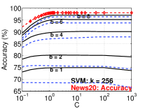
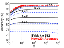
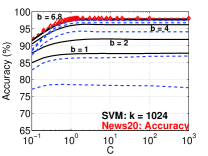
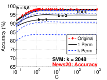
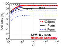
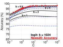
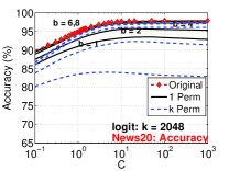
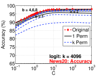
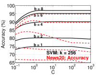
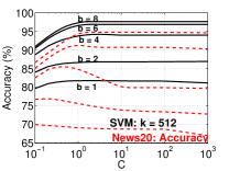
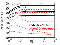
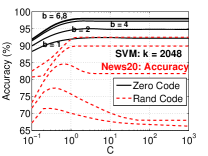
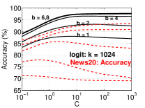
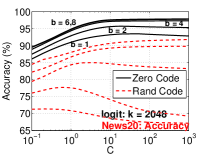
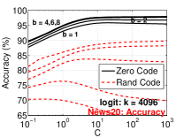
To test the robustness of one permutation hashing, we also experiment with the news20 dataset, which has only 20,000 samples and 1,355,191 features, with merely about 500 nonzeros per feature vector on average. We purposely let k𝑘k be as large as 409640964096. Interestingly, the experimental results show that the zero coding strategy can perform extremely well. The test accuracies consistently improve as k𝑘k increases. In comparisons, the random coding strategy performs badly unless k𝑘k is small (e.g., k256𝑘256k\leq 256).

On the news20 dataset, our one permutation scheme actually outperforms the original k𝑘k-permutation scheme, quite noticeably when k𝑘k is large. This should be due to the benefits from the “sample-without-replacement” effect. One permutation hashing provides a good matrix sparsification scheme without “damaging” the original data matrix too much.

5 Experimental Results on the Webspam Dataset

The webspam dataset has 350,000 samples and 16,609,143 features. Each feature vector has on average about 4000 nonzeros; see Figure 9. Following [18], we use 80%percent8080\% of samples for training and the remaining 20%percent2020\% for testing. We conduct extensive experiments on linear SVM and logistic regression, using our proposed one permutation hashing scheme with k{25,26,27,28,29}𝑘superscript25superscript26superscript27superscript28superscript29k\in\{2^{5},2^{6},2^{7},2^{8},2^{9}\} and b{1,2,4,6,8}𝑏12468b\in\{1,2,4,6,8\}. For convenience, we use D=224𝐷superscript224D=2^{24}, which is divisible by k𝑘k and is slightly larger than 16,609,143.

There is one regularization parameter C𝐶C in linear SVM and logistic regression. Since our purpose is to demonstrate the effectiveness of our proposed hashing scheme, we simply provide the results for a wide range of C𝐶C values and assume that the best performance is achievable if we conduct cross-validations. This way, interested readers may be able to easily reproduce our experiments.

5.1 One Permutation v.s. k-Permutation

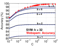
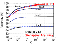
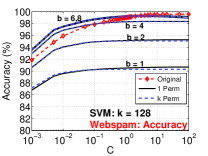
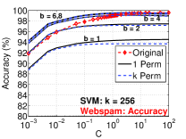
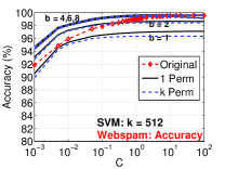
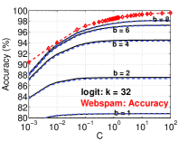
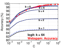
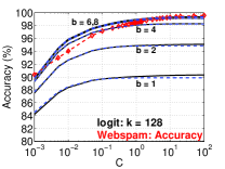
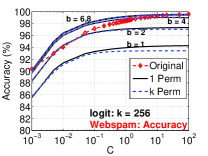
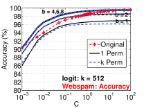
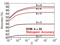
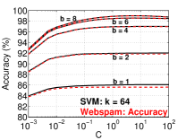
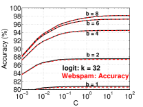
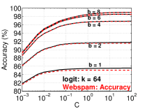
Figure 10 presents the test accuracies for both linear SVM (upper panels) and logistic regression (bottom panels). Clearly, when k=512𝑘512k=512 (or even 256) and b=8𝑏8b=8, b𝑏b-bit one permutation hashing achieves similar test accuracies as using the original data. Also, compared to the original k𝑘k-permutation scheme as in [18], our one permutation scheme achieves similar (or even very slightly better) accuracies.

Refer to caption Refer to caption Refer to caption Refer to caption Refer to caption

Refer to caption Refer to caption Refer to caption Refer to caption Refer to caption

Figure 10: Test accuracies of SVM (upper panels) and logistic regression (bottom panels), averaged over 50 repetitions. The accuracies of using the original data are plotted as dashed (red, if color is available) curves with “diamond” markers. C𝐶C is the regularization parameter. Compared with the original k𝑘k-permutation minwise hashing scheme (dashed and blue if color is available), the proposed one permutation hashing scheme achieves very similar accuracies, or even slightly better accuracies when k𝑘k is large.

5.2 Preprocessing Time and Training Time

The preprocessing cost for processing the data using k=512𝑘512k=512 independent permutations is about 6,000 seconds. In contrast, the processing cost for the proposed one permutation scheme is only 1/k1𝑘1/k of the original cost, i.e., about 10 seconds. Note that webspam is merely a small dataset compared to industrial applications. We expect the (absolute) improvement will be even more substantial in much larger datasets.

The prior work [18] already presented the training time using the k𝑘k-permutation hashing scheme. With one permutation hashing, the training time remains essentially the same (for the same k𝑘k and b𝑏b) on the webspam dataset. Note that, with the zero coding strategy, the new data matrix generated by one permutation hashing has potentially less nonzeros than the original minwise hashing scheme, due to the occurrences of empty bins. This phenomenon in theory may bring additional advantages such as slightly reducing the training time. Nevertheless, the most significant advantage of one permutation hashing lies in the dramatic reduction of the preprocessing cost, which is what we focus on in this study.

5.3 Zero Coding v.s. Random Coding for Empty Bins

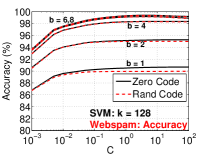
The experimental results as shown in Figure 10 are based on the “zero coding” strategy for dealing with empty bins. Figure 11 plots the results for comparing zero coding with the random coding. When k𝑘k is large, zero coding is superior to random coding, although the differences remain small in this dataset. This is not surprising, of course. Random coding adds artificial nonzeros to the new (expanded) data matrix, which would not be desirable for learning algorithms.
Refer to caption Refer to caption Refer to caption Refer to caption Refer to caption

Refer to caption Refer to caption Refer to caption Refer to caption Refer to caption

Figure 11: Test accuracies of SVM (upper panels) and logistic regression (bottom panels), averaged over 50 repetitions, for comparing the (recommended) zero coding strategy with the random coding strategy to deal with empty bins. We can see that the differences only become noticeable at k=512𝑘512k=512.
Remark: The empirical results on the webspam datasets are highly encouraging because they verify that our proposed one permutation hashing scheme works as well as (or even slightly better than) the original k𝑘k-permutation scheme, at merely 1/k1𝑘1/k of the original preprocessing cost. On the other hand, it would be more interesting, from the perspective of testing the robustness of our algorithm, to conduct experiments on a dataset where the empty bins will occur much more frequently.

6 Experimental Results on the News20 Dataset

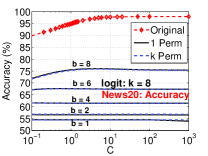
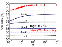
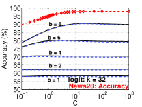
The news20 dataset (with 20,000 samples and 1,355,191 features) is a very small dataset in not-too-high dimensions. The average number of nonzeros per feature vector is about 500, which is also small. Therefore, this is more like a contrived example and we use it just to verify that our one permutation scheme (with the zero coding strategy) still works very well even when we let k𝑘k be as large as 4096 (i.e., most of the bins are empty). In fact, the one permutation schemes achieves noticeably better accuracies than the original k𝑘k-permutation scheme. We believe this is because the one permutation scheme is “sample-without-replacement” and provides a much better matrix sparsification strategy without “contaminating” the original data matrix too much.

6.1 One Permutation v.s. k-Permutation

We experiment with k{23,24,25,26,27,28,29,210,211,212}𝑘superscript23superscript24superscript25superscript26superscript27superscript28superscript29superscript210superscript211superscript212k\in\{2^{3},2^{4},2^{5},2^{6},2^{7},2^{8},2^{9},2^{10},2^{11},2^{12}\} and b{1,2,4,6,8}𝑏12468b\in\{1,2,4,6,8\}, for both one permutation scheme and k𝑘k-permutation scheme. We use 10,000 samples for training and the other 10,000 samples for testing. For convenience, we let D=221𝐷superscript221D=2^{21} (which is larger than 1,355,191).

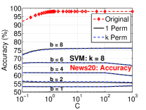
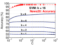
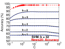
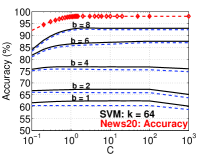
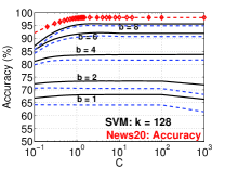
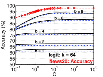
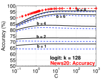
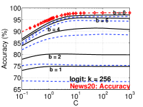
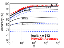
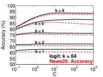
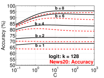
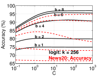
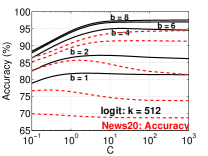
Figure 12 and Figure 13 present the test accuracies for linear SVM and logistic regression, respectively. When k𝑘k is small (e.g., k64𝑘64k\leq 64) both the one permutation scheme and the original k𝑘k-permutation scheme perform similarly. For larger k𝑘k values (especially as k256𝑘256k\geq 256), however, our one permutation scheme noticeably outperforms the k𝑘k-permutation scheme. Using the original data, the test accuracies are about 98%percent9898\%. Our one permutation scheme with k512𝑘512k\geq 512 and b=8𝑏8b=8 essentially achieves the original test accuracies, while the k𝑘k-permutation scheme could only reach about 97.5%percent97.597.5\% even with k=4096𝑘4096k=4096.

Refer to caption Refer to caption Refer to caption Refer to caption Refer to caption

Refer to caption Refer to caption Refer to caption Refer to caption Refer to caption

Figure 12: Test accuracies of linear SVM averaged over 100 repetitions. The proposed one permutation scheme noticeably outperforms the original k𝑘k-permutation scheme especially when k𝑘k is not small.

Refer to caption Refer to caption Refer to caption Refer to caption Refer to caption

Refer to caption Refer to caption Refer to caption Refer to caption Refer to caption

Figure 13: Test accuracies of logistic regression averaged over 100 repetitions. The proposed one permutation scheme noticeably outperforms the original k𝑘k-permutation scheme especially when k𝑘k is not small.

6.2 Zero Coding v.s. Random Coding for Empty Bins

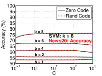
Figure 14 and Figure 15 plot the results for comparing two coding strategies to deal with empty bins, respectively for linear SVM and logistic regression. Again, when k𝑘k is small (e.g., k64𝑘64k\leq 64), both strategies perform similarly. However, when k𝑘k is large, using the random coding scheme may be disastrous, which is of course also expected. When k=4096𝑘4096k=4096, most of the nonzero entries in the new expanded data matrix fed to the solver are artificial, since the original news20 dataset has merely about 500500500 nonzero on average.

Refer to caption Refer to caption Refer to caption Refer to caption Refer to caption

Refer to caption Refer to caption Refer to caption Refer to caption Refer to caption

Figure 14: Test accuracies of linear SVM averaged over 100 repetitions, for comparing the (recommended) zero coding strategy with the random coding strategy to deal with empty bins. On this dataset, the performance of the random coding strategy can be bad.
Refer to caption Refer to caption Refer to caption Refer to caption Refer to caption

Refer to caption Refer to caption Refer to caption Refer to caption Refer to caption

Figure 15: Test accuracies of logistic regression averaged over 100 repetitions, for comparing the zero coding strategy (recommended) with the random coding strategy to deal with empty bins. On this dataset, the performance of the random coding strategy can be bad.
Remark: We should re-iterate that the news20 dataset is more like a contrived example, merely for testing the robustness of the one permutation scheme with the zero coding strategy. In more realistic industrial applications, we expect that numbers of nonzeros in many datasets should be significantly higher, and hence the performance differences between the one permutation scheme and the k𝑘k-permutation scheme and the differences between the two strategies for empty bins should be small.

7 The Variable Length One Permutation Hashing Scheme

While the fixed-length one permutation scheme we have presented and analyzed should be simple to implement and easy to understand, we would like to present a variable-length scheme which may more obviously connect with other known hashing methods such as the Count-Min (CM) sketch [6].

As in the fixed-length scheme, we first conduct a permutation π:ΩΩ:𝜋ΩΩ\pi:\Omega\rightarrow\Omega. Instead of dividing the space evenly, we vary the bin lengths according to a multinomial distribution mult(D,1k,1k,,1k)𝑚𝑢𝑙𝑡𝐷1𝑘1𝑘1𝑘mult\left(D,\frac{1}{k},\frac{1}{k},...,\frac{1}{k}\right).

This variable-length scheme is equivalent to first uniformly grouping the original data entries into k𝑘k bins and then applying permutations independently within each bin. The latter explanation connects our method with the Count-Min (CM) sketch [6] (but without the “count-min” step), which also hashes the elements uniformly to k𝑘k bins and the final (stored) hashed value in each bin is the sum of all the elements in the bin. The bias of the CM estimate can be removed by subtracting a term. [20] adopted the CM sketch for linear learning. Later, [24] proposed a novel idea (named “VW”) to remove the bias, by pre-multiplying (element-wise) the original data vectors with a random vector whose entries are sampled i.i.d. from the two-point distribution in {1,1}11\{-1,1\} with equal probabilities. In a recent paper, [18] showed that the variance of the CM sketch and variants are equivalent to the variance of random projections [16], which is substantially larger than the variance of the minwise hashing when the data are binary.

Since [18] has already conducted (theoretical and empirical) comparisons with CM and VW methods, we do not include more comparisons in this paper. Instead, we have simply showed that with one permutation only, we are able to achieve essentially the same accuracy as using k𝑘k permutations.

We believe the fixed-length scheme is more convenient to implement. Nevertheless, we would like to present some theoretical results for the variable-length scheme, for better understanding the differences. The major difference is the distribution of Nempsubscript𝑁𝑒𝑚𝑝N_{emp}, the number of jointly empty bins.
Lemma 8

Under the variable-length scheme,

E(Nemp)k=𝐸subscript𝑁𝑒𝑚𝑝𝑘absent\displaystyle\frac{E\left(N_{emp}\right)}{k}= (11k)f1+f2asuperscript11𝑘subscript𝑓1subscript𝑓2𝑎\displaystyle\left(1-\frac{1}{k}\right)^{f_{1}+f_{2}-a} (45)
Var(Nemp)k2=𝑉𝑎𝑟subscript𝑁𝑒𝑚𝑝superscript𝑘2absent\displaystyle\frac{Var\left(N_{emp}\right)}{k^{2}}= 1k(E(Nemp)k)(1E(Nemp)k)1𝑘𝐸subscript𝑁𝑒𝑚𝑝𝑘1𝐸subscript𝑁𝑒𝑚𝑝𝑘\displaystyle\frac{1}{k}\left(\frac{E(N_{emp})}{k}\right)\left(1-\frac{E(N_{emp})}{k}\right) (46)
(11k)((11k)2(f1+f2a)(12k)f1+f2a)11𝑘superscript11𝑘2subscript𝑓1subscript𝑓2𝑎superscript12𝑘subscript𝑓1subscript𝑓2𝑎\displaystyle-\left(1-\frac{1}{k}\right)\left(\left(1-\frac{1}{k}\right)^{2(f_{1}+f_{2}-a)}-\left(1-\frac{2}{k}\right)^{f_{1}+f_{2}-a}\right)
<\displaystyle< 1k(E(Nemp)k)(1E(Nemp)k)1𝑘𝐸subscript𝑁𝑒𝑚𝑝𝑘1𝐸subscript𝑁𝑒𝑚𝑝𝑘\displaystyle\frac{1}{k}\left(\frac{E(N_{emp})}{k}\right)\left(1-\frac{E(N_{emp})}{k}\right) (47)

Proof: See Appendix H. \Box

The other theoretical results for the fixed-length scheme which are expressed in terms Nempsubscript𝑁𝑒𝑚𝑝N_{emp} essentially hold for the variable-length scheme. For example, NmatkNempsubscript𝑁𝑚𝑎𝑡𝑘subscript𝑁𝑒𝑚𝑝\frac{N_{mat}}{k-N_{emp}} is still an unbiased estimator of R𝑅R and its variance is in the same form as (35) in terms of Nempsubscript𝑁𝑒𝑚𝑝N_{emp}.

Remark:     The number of empty bins for the variable-length scheme as presented in (45) is actually an upper bound of the number of empty bins for the fixed length scheme as shown in (21). The difference between j=0f1D(11k)jDjsuperscriptsubscriptproduct𝑗0𝑓1𝐷11𝑘𝑗𝐷𝑗\prod_{j=0}^{f-1}\frac{D\left(1-\frac{1}{k}\right)-j}{D-j} and (11k)fsuperscript11𝑘𝑓\left(1-\frac{1}{k}\right)^{f} (recall f=f1+f2a𝑓subscript𝑓1subscript𝑓2𝑎f=f_{1}+f_{2}-a) is small when the data are sparse, as shown in Lemma 2, although it is possible that j=0f1D(11k)jDj(11k)fmuch-less-thansuperscriptsubscriptproduct𝑗0𝑓1𝐷11𝑘𝑗𝐷𝑗superscript11𝑘𝑓\prod_{j=0}^{f-1}\frac{D\left(1-\frac{1}{k}\right)-j}{D-j}\ll\left(1-\frac{1}{k}\right)^{f} in corner cases. Because smaller Nempsubscript𝑁𝑒𝑚𝑝N_{emp} implies potentially better performance, we conclude that the fixed-length scheme should be sufficient and there are perhaps no practical needs to use the variable-length scheme.

8 Conclusion

A new hashing algorithm is developed for large-scale search and learning in massive binary data. Compared with the original k𝑘k-permutation (e.g., k=500𝑘500k=500) minwise hashing algorithm (which is the standard procedure in the context of search), our method requires only one permutation and can achieve similar or even better accuracies at merely 1/k1𝑘1/k of the original preprocessing cost. We expect that our proposed algorithm (or its variant) will be adopted in practice.

References

  • [1] Alexandr Andoni and Piotr Indyk. Near-optimal hashing algorithms for approximate nearest neighbor in high dimensions. In Commun. ACM, volume 51, pages 117–122, 2008.
  • [2] Leon Bottou. http://leon.bottou.org/projects/sgd.
  • [3] Andrei Z. Broder, Moses Charikar, Alan M. Frieze, and Michael Mitzenmacher. Min-wise independent permutations (extended abstract). In STOC, pages 327–336, Dallas, TX, 1998.
  • [4] Andrei Z. Broder, Steven C. Glassman, Mark S. Manasse, and Geoffrey Zweig. Syntactic clustering of the web. In WWW, pages 1157 – 1166, Santa Clara, CA, 1997.
  • [5] J. Lawrence Carter and Mark N. Wegman. Universal classes of hash functions (extended abstract). In STOC, pages 106–112, 1977.
  • [6] Graham Cormode and S. Muthukrishnan. An improved data stream summary: the count-min sketch and its applications. Journal of Algorithm, 55(1):58–75, 2005.
  • [7] Rong-En Fan, Kai-Wei Chang, Cho-Jui Hsieh, Xiang-Rui Wang, and Chih-Jen Lin. Liblinear: A library for large linear classification. Journal of Machine Learning Research, 9:1871–1874, 2008.
  • [8] Dennis Fetterly, Mark Manasse, Marc Najork, and Janet L. Wiener. A large-scale study of the evolution of web pages. In WWW, pages 669–678, Budapest, Hungary, 2003.
  • [9] Jerome H. Friedman, F. Baskett, and L. Shustek. An algorithm for finding nearest neighbors. IEEE Transactions on Computers, 24:1000–1006, 1975.
  • [10] Izrail S. Gradshteyn and Iosif M. Ryzhik. Table of Integrals, Series, and Products. Academic Press, New York, sixth edition, 2000.
  • [11] Cho-Jui Hsieh, Kai-Wei Chang, Chih-Jen Lin, S. Sathiya Keerthi, and S. Sundararajan. A dual coordinate descent method for large-scale linear svm. In Proceedings of the 25th international conference on Machine learning, ICML, pages 408–415, 2008.
  • [12] Piotr Indyk and Rajeev Motwani. Approximate nearest neighbors: Towards removing the curse of dimensionality. In STOC, pages 604–613, Dallas, TX, 1998.
  • [13] Thorsten Joachims. Training linear svms in linear time. In KDD, pages 217–226, Pittsburgh, PA, 2006.
  • [14] Ping Li and Kenneth W. Church. Using sketches to estimate associations. In HLT/EMNLP, pages 708–715, Vancouver, BC, Canada, 2005 (The full paper appeared in Commputational Linguistics in 2007).
  • [15] Ping Li, Kenneth W. Church, and Trevor J. Hastie. One sketch for all: Theory and applications of conditional random sampling. In NIPS (Preliminary results appeared in NIPS 2006), Vancouver, BC, Canada, 2008.
  • [16] Ping Li, Trevor J. Hastie, and Kenneth W. Church. Very sparse random projections. In KDD, pages 287–296, Philadelphia, PA, 2006.
  • [17] Ping Li and Arnd Christian König. Theory and applications b-bit minwise hashing. Commun. ACM, 2011.
  • [18] Ping Li, Anshumali Shrivastava, Joshua Moore, and Arnd Christian König. Hashing algorithms for large-scale learning. In NIPS, Granada, Spain, 2011.
  • [19] Shai Shalev-Shwartz, Yoram Singer, and Nathan Srebro. Pegasos: Primal estimated sub-gradient solver for svm. In ICML, pages 807–814, Corvalis, Oregon, 2007.
  • [20] Qinfeng Shi, James Petterson, Gideon Dror, John Langford, Alex Smola, and S.V.N. Vishwanathan. Hash kernels for structured data. Journal of Machine Learning Research, 10:2615–2637, 2009.
  • [21] Anshumali Shrivastava and Ping Li. Fast near neighbor search in high-dimensional binary data. In ECML, 2012.
  • [22] Josef Sivic and Andrew Zisserman. Video google: a text retrieval approach to object matching in videos. In ICCV, 2003.
  • [23] Simon Tong. Lessons learned developing a practical large scale machine learning system. http://googleresearch.blogspot.com/2010/04/lessons-learned-developing-practical.html, 2008.
  • [24] Kilian Weinberger, Anirban Dasgupta, John Langford, Alex Smola, and Josh Attenberg. Feature hashing for large scale multitask learning. In ICML, pages 1113–1120, 2009.

Appendix A Proof of Lemma 1

Recall Nemp=j=1kIemp,jsubscript𝑁𝑒𝑚𝑝superscriptsubscript𝑗1𝑘subscript𝐼𝑒𝑚𝑝𝑗N_{emp}=\sum_{j=1}^{k}I_{emp,j}, where Iemp,j=1subscript𝐼𝑒𝑚𝑝𝑗1I_{emp,j}=1 if, in the j𝑗j-th bin, both π(S1)𝜋subscript𝑆1\pi(S_{1}) and π(S2)𝜋subscript𝑆2\pi(S_{2}) are empty, and Iemp,j=0subscript𝐼𝑒𝑚𝑝𝑗0I_{emp,j}=0 otherwise. Also recall D=|Ω|𝐷ΩD=|\Omega|, f1=|S1|subscript𝑓1subscript𝑆1f_{1}=|S_{1}|, f2=|S2|subscript𝑓2subscript𝑆2f_{2}=|S_{2}|, a=|S1S2|𝑎subscript𝑆1subscript𝑆2a=|S_{1}\cap S_{2}|. Obviously, if D(11k)<f1+f2a𝐷11𝑘subscript𝑓1subscript𝑓2𝑎D\left(1-\frac{1}{k}\right)<f_{1}+f_{2}-a, then none of the bins will be jointly empty, i.e., E(Nemp)=Var(Nemp)=0𝐸subscript𝑁𝑒𝑚𝑝𝑉𝑎𝑟subscript𝑁𝑒𝑚𝑝0E(N_{emp})=Var(N_{emp})=0. Next, assume D(11k)f1+f2a𝐷11𝑘subscript𝑓1subscript𝑓2𝑎D\left(1-\frac{1}{k}\right)\geq f_{1}+f_{2}-a, then by the linearity of expectation,

E(Nemp)=j=1k𝐏𝐫(Iemp,j=1)=k𝐏𝐫(Iemp,1=1)=k(D(11k)f1+f2a)(Df1+f2a)=kj=0f1+f2a1D(11k)jDj𝐸subscript𝑁𝑒𝑚𝑝superscriptsubscript𝑗1𝑘𝐏𝐫subscript𝐼𝑒𝑚𝑝𝑗1𝑘𝐏𝐫subscript𝐼𝑒𝑚𝑝11𝑘binomial𝐷11𝑘subscript𝑓1subscript𝑓2𝑎binomial𝐷subscript𝑓1subscript𝑓2𝑎𝑘superscriptsubscriptproduct𝑗0subscript𝑓1subscript𝑓2𝑎1𝐷11𝑘𝑗𝐷𝑗\displaystyle E\left(N_{emp}\right)=\sum_{j=1}^{k}\mathbf{Pr}\left(I_{emp,j}=1\right)=k\mathbf{Pr}\left(I_{emp,1}=1\right)=k\frac{\binom{D\left(1-\frac{1}{k}\right)}{f_{1}+f_{2}-a}}{\binom{D}{f_{1}+f_{2}-a}}=k\prod_{j=0}^{f_{1}+f_{2}-a-1}\frac{D\left(1-\frac{1}{k}\right)-j}{D-j}

To derive the variance, we first assume D(12k)f1+f2a𝐷12𝑘subscript𝑓1subscript𝑓2𝑎D\left(1-\frac{2}{k}\right)\geq f_{1}+f_{2}-a. Then

Var(Nemp)=𝑉𝑎𝑟subscript𝑁𝑒𝑚𝑝absent\displaystyle Var\left(N_{emp}\right)= E(Nemp2)E2(Nemp)𝐸superscriptsubscript𝑁𝑒𝑚𝑝2superscript𝐸2subscript𝑁𝑒𝑚𝑝\displaystyle E\left(N_{emp}^{2}\right)-E^{2}\left(N_{emp}\right)
=\displaystyle= E(j=1kIemp,j2+ijIemp,iIemp,j)E2(Nemp)𝐸superscriptsubscript𝑗1𝑘superscriptsubscript𝐼𝑒𝑚𝑝𝑗2subscript𝑖𝑗subscript𝐼𝑒𝑚𝑝𝑖subscript𝐼𝑒𝑚𝑝𝑗superscript𝐸2subscript𝑁𝑒𝑚𝑝\displaystyle E\left(\sum_{j=1}^{k}I_{emp,j}^{2}+\sum_{i\neq j}I_{emp,i}I_{emp,j}\right)-E^{2}\left(N_{emp}\right)
=\displaystyle= k(k1)𝐏𝐫(Iemp,1=1,Iemp,2=1)+E(Nemp)E2(Nemp)𝑘𝑘1𝐏𝐫formulae-sequencesubscript𝐼𝑒𝑚𝑝11subscript𝐼𝑒𝑚𝑝21𝐸subscript𝑁𝑒𝑚𝑝superscript𝐸2subscript𝑁𝑒𝑚𝑝\displaystyle k(k-1)\mathbf{Pr}\left(I_{emp,1}=1,I_{emp,2}=1\right)+E\left(N_{emp}\right)-E^{2}\left(N_{emp}\right)
=\displaystyle= k(k1)×j=0f1+f2a1D(12k)jDj𝑘𝑘1superscriptsubscriptproduct𝑗0subscript𝑓1subscript𝑓2𝑎1𝐷12𝑘𝑗𝐷𝑗\displaystyle k(k-1)\times\prod_{j=0}^{f_{1}+f_{2}-a-1}\frac{D\left(1-\frac{2}{k}\right)-j}{D-j}
+k×j=0f1+f2a1D(11k)jDj(k×j=0f1+f2a1D(11k)jDj)2𝑘superscriptsubscriptproduct𝑗0subscript𝑓1subscript𝑓2𝑎1𝐷11𝑘𝑗𝐷𝑗superscript𝑘superscriptsubscriptproduct𝑗0subscript𝑓1subscript𝑓2𝑎1𝐷11𝑘𝑗𝐷𝑗2\displaystyle+k\times\prod_{j=0}^{f_{1}+f_{2}-a-1}\frac{D\left(1-\frac{1}{k}\right)-j}{D-j}-\left(k\times\prod_{j=0}^{f_{1}+f_{2}-a-1}\frac{D\left(1-\frac{1}{k}\right)-j}{D-j}\right)^{2}

If D(12k)<f1+f2aD(11k)𝐷12𝑘subscript𝑓1subscript𝑓2𝑎𝐷11𝑘D\left(1-\frac{2}{k}\right)<f_{1}+f_{2}-a\leq D\left(1-\frac{1}{k}\right), then 𝐏𝐫(Iemp,1=1,Iemp,2=1)=0𝐏𝐫formulae-sequencesubscript𝐼𝑒𝑚𝑝11subscript𝐼𝑒𝑚𝑝210\mathbf{Pr}\left(I_{emp,1}=1,I_{emp,2}=1\right)=0 and hence

Var(Nemp)=E(Nemp)E2(Nemp)=k×j=0f1+f2a1D(11k)jDj(k×j=0f1+f2a1D(11k)jDj)2𝑉𝑎𝑟subscript𝑁𝑒𝑚𝑝𝐸subscript𝑁𝑒𝑚𝑝superscript𝐸2subscript𝑁𝑒𝑚𝑝𝑘superscriptsubscriptproduct𝑗0subscript𝑓1subscript𝑓2𝑎1𝐷11𝑘𝑗𝐷𝑗superscript𝑘superscriptsubscriptproduct𝑗0subscript𝑓1subscript𝑓2𝑎1𝐷11𝑘𝑗𝐷𝑗2\displaystyle Var\left(N_{emp}\right)=E\left(N_{emp}\right)-E^{2}\left(N_{emp}\right)=k\times\prod_{j=0}^{f_{1}+f_{2}-a-1}\frac{D\left(1-\frac{1}{k}\right)-j}{D-j}-\left(k\times\prod_{j=0}^{f_{1}+f_{2}-a-1}\frac{D\left(1-\frac{1}{k}\right)-j}{D-j}\right)^{2}

Assuming D(12k)f1+f2a𝐷12𝑘subscript𝑓1subscript𝑓2𝑎D\left(1-\frac{2}{k}\right)\geq f_{1}+f_{2}-a, we obtain

Var(Nemp)k2=𝑉𝑎𝑟subscript𝑁𝑒𝑚𝑝superscript𝑘2absent\displaystyle\frac{Var\left(N_{emp}\right)}{k^{2}}= 1k(j=0f1+f2a1D(11k)jDj)(1j=0f1+f2a1D(11k)jDj)1𝑘superscriptsubscriptproduct𝑗0subscript𝑓1subscript𝑓2𝑎1𝐷11𝑘𝑗𝐷𝑗1superscriptsubscriptproduct𝑗0subscript𝑓1subscript𝑓2𝑎1𝐷11𝑘𝑗𝐷𝑗\displaystyle\frac{1}{k}\left(\prod_{j=0}^{f_{1}+f_{2}-a-1}\frac{D\left(1-\frac{1}{k}\right)-j}{D-j}\right)\left(1-\prod_{j=0}^{f_{1}+f_{2}-a-1}\frac{D\left(1-\frac{1}{k}\right)-j}{D-j}\right)
(11k)((j=0f1+f2a1D(11k)jDj)2j=0f1+f2a1D(12k)jDj)11𝑘superscriptsuperscriptsubscriptproduct𝑗0subscript𝑓1subscript𝑓2𝑎1𝐷11𝑘𝑗𝐷𝑗2superscriptsubscriptproduct𝑗0subscript𝑓1subscript𝑓2𝑎1𝐷12𝑘𝑗𝐷𝑗\displaystyle-\left(1-\frac{1}{k}\right)\left(\left(\prod_{j=0}^{f_{1}+f_{2}-a-1}\frac{D\left(1-\frac{1}{k}\right)-j}{D-j}\right)^{2}-\prod_{j=0}^{f_{1}+f_{2}-a-1}\frac{D\left(1-\frac{2}{k}\right)-j}{D-j}\right)
=\displaystyle= 1k(E(Nemp)k)(1E(Nemp)k)1𝑘𝐸subscript𝑁𝑒𝑚𝑝𝑘1𝐸subscript𝑁𝑒𝑚𝑝𝑘\displaystyle\frac{1}{k}\left(\frac{E(N_{emp})}{k}\right)\left(1-\frac{E(N_{emp})}{k}\right)
(11k)((j=0f1+f2a1D(11k)jDj)2j=0f1+f2a1D(12k)jDj)11𝑘superscriptsuperscriptsubscriptproduct𝑗0subscript𝑓1subscript𝑓2𝑎1𝐷11𝑘𝑗𝐷𝑗2superscriptsubscriptproduct𝑗0subscript𝑓1subscript𝑓2𝑎1𝐷12𝑘𝑗𝐷𝑗\displaystyle-\left(1-\frac{1}{k}\right)\left(\left(\prod_{j=0}^{f_{1}+f_{2}-a-1}\frac{D\left(1-\frac{1}{k}\right)-j}{D-j}\right)^{2}-\prod_{j=0}^{f_{1}+f_{2}-a-1}\frac{D\left(1-\frac{2}{k}\right)-j}{D-j}\right)
<\displaystyle< 1k(E(Nemp)k)(1E(Nemp)k)1𝑘𝐸subscript𝑁𝑒𝑚𝑝𝑘1𝐸subscript𝑁𝑒𝑚𝑝𝑘\displaystyle\frac{1}{k}\left(\frac{E(N_{emp})}{k}\right)\left(1-\frac{E(N_{emp})}{k}\right)

because

(D(11k)jDj)2D(12k)jDj>0superscript𝐷11𝑘𝑗𝐷𝑗2𝐷12𝑘𝑗𝐷𝑗0\displaystyle\left(\frac{D\left(1-\frac{1}{k}\right)-j}{D-j}\right)^{2}-\frac{D\left(1-\frac{2}{k}\right)-j}{D-j}>0
\displaystyle\Longleftrightarrow (D(11k)j)2>(Dj)(D(12k)j)superscript𝐷11𝑘𝑗2𝐷𝑗𝐷12𝑘𝑗\displaystyle\left(D\left(1-\frac{1}{k}\right)-j\right)^{2}>(D-j)\left(D\left(1-\frac{2}{k}\right)-j\right)
\displaystyle\Longleftrightarrow (11k)2=12k+1k2>12ksuperscript11𝑘212𝑘1superscript𝑘212𝑘\displaystyle\left(1-\frac{1}{k}\right)^{2}=1-\frac{2}{k}+\frac{1}{k^{2}}>1-\frac{2}{k}

This completes the proof.

Appendix B Proof of Lemma 2

The following expansions will be useful

j=1n11j=logn+0.57721612n112n2+([10, 8.367.13])superscriptsubscript𝑗1𝑛11𝑗𝑛0.57721612𝑛112superscript𝑛2[10, 8.367.13]\displaystyle\sum_{j=1}^{n-1}\frac{1}{j}=\log n+0.577216-\frac{1}{2n}-\frac{1}{12n^{2}}+...\hskip 36.135pt(\text{\cite[cite]{[\@@bibref{}{Book:Gradshteyn_00}{}{}, 8.367.13]}}) (48)
log(1x)=xx22x33(|x|<1)1𝑥𝑥superscript𝑥22superscript𝑥33𝑥1\displaystyle\log(1-x)=-x-\frac{x^{2}}{2}-\frac{x^{3}}{3}-...\hskip 36.135pt(|x|<1) (49)

Assume D(11k)f1+f2a𝐷11𝑘subscript𝑓1subscript𝑓2𝑎D\left(1-\frac{1}{k}\right)\geq f_{1}+f_{2}-a. We can write

E(Nemp)k=𝐸subscript𝑁𝑒𝑚𝑝𝑘absent\displaystyle\frac{E\left(N_{emp}\right)}{k}= j=0f1+f2a1D(11k)jDj=(11k)f1+f2a×j=0f1+f2a1(1j(k1)(Dj))superscriptsubscriptproduct𝑗0subscript𝑓1subscript𝑓2𝑎1𝐷11𝑘𝑗𝐷𝑗superscript11𝑘subscript𝑓1subscript𝑓2𝑎superscriptsubscriptproduct𝑗0subscript𝑓1subscript𝑓2𝑎11𝑗𝑘1𝐷𝑗\displaystyle\prod_{j=0}^{f_{1}+f_{2}-a-1}\frac{D\left(1-\frac{1}{k}\right)-j}{D-j}=\left(1-\frac{1}{k}\right)^{f_{1}+f_{2}-a}\times\prod_{j=0}^{f_{1}+f_{2}-a-1}\left(1-\frac{j}{(k-1)(D-j)}\right)

Hence it suffices to study the error term

j=0f1+f2a1(1j(k1)(Dj)).superscriptsubscriptproduct𝑗0subscript𝑓1subscript𝑓2𝑎11𝑗𝑘1𝐷𝑗\displaystyle\prod_{j=0}^{f_{1}+f_{2}-a-1}\left(1-\frac{j}{(k-1)(D-j)}\right).
logj=0f1+f2a1(1j(k1)(Dj))=j=0f1+f2a1log(1j(k1)(Dj))superscriptsubscriptproduct𝑗0subscript𝑓1subscript𝑓2𝑎11𝑗𝑘1𝐷𝑗superscriptsubscript𝑗0subscript𝑓1subscript𝑓2𝑎11𝑗𝑘1𝐷𝑗\displaystyle\log\prod_{j=0}^{f_{1}+f_{2}-a-1}\left(1-\frac{j}{(k-1)(D-j)}\right)=\sum_{j=0}^{f_{1}+f_{2}-a-1}\log\left(1-\frac{j}{(k-1)(D-j)}\right)
=\displaystyle= j=0f1+f2a1{j(k1)(Dj)12(j(k1)(Dj))213(j(k1)(Dj))3+}superscriptsubscript𝑗0subscript𝑓1subscript𝑓2𝑎1𝑗𝑘1𝐷𝑗12superscript𝑗𝑘1𝐷𝑗213superscript𝑗𝑘1𝐷𝑗3\displaystyle\sum_{j=0}^{f_{1}+f_{2}-a-1}\left\{-\frac{j}{(k-1)(D-j)}-\frac{1}{2}\left(\frac{j}{(k-1)(D-j)}\right)^{2}-\frac{1}{3}\left(\frac{j}{(k-1)(D-j)}\right)^{3}+...\right\}

Take the first term,

j=0f1+f2a1j(k1)(Dj)=1k1j=0f1+f2a1DjDjDDjsuperscriptsubscript𝑗0subscript𝑓1subscript𝑓2𝑎1𝑗𝑘1𝐷𝑗1𝑘1superscriptsubscript𝑗0subscript𝑓1subscript𝑓2𝑎1𝐷𝑗𝐷𝑗𝐷𝐷𝑗\displaystyle\sum_{j=0}^{f_{1}+f_{2}-a-1}-\frac{j}{(k-1)(D-j)}=\frac{1}{k-1}\sum_{j=0}^{f_{1}+f_{2}-a-1}\frac{D-j}{D-j}-\frac{D}{D-j}
=\displaystyle= 1k1(f1+f2aDj=0f1+f2a11Dj)1𝑘1subscript𝑓1subscript𝑓2𝑎𝐷superscriptsubscript𝑗0subscript𝑓1subscript𝑓2𝑎11𝐷𝑗\displaystyle\frac{1}{k-1}\left(f_{1}+f_{2}-a-D\sum_{j=0}^{f_{1}+f_{2}-a-1}\frac{1}{D-j}\right)
=\displaystyle= 1k1(f1+f2aD(j=1D1jj=1Df1f2+a1j))1𝑘1subscript𝑓1subscript𝑓2𝑎𝐷superscriptsubscript𝑗1𝐷1𝑗superscriptsubscript𝑗1𝐷subscript𝑓1subscript𝑓2𝑎1𝑗\displaystyle\frac{1}{k-1}\left(f_{1}+f_{2}-a-D\left(\sum_{j=1}^{D}\frac{1}{j}-\sum_{j=1}^{D-f_{1}-f_{2}+a}\frac{1}{j}\right)\right)
=\displaystyle= 1k1(f1+f2aD(log(D+1)12(D+1)log(Df1f2+a+1)+12(Df1f2+a+1))+)1𝑘1subscript𝑓1subscript𝑓2𝑎𝐷𝐷112𝐷1𝐷subscript𝑓1subscript𝑓2𝑎112𝐷subscript𝑓1subscript𝑓2𝑎1\displaystyle\frac{1}{k-1}\left(f_{1}+f_{2}-a-D\left(\log(D+1)-\frac{1}{2(D+1)}-\log(D-f_{1}-f_{2}+a+1)+\frac{1}{2(D-f_{1}-f_{2}+a+1)}\right)+...\right)

Thus, we obtain (by ignoring a term DD+1𝐷𝐷1\frac{D}{D+1})

j=0f1+f2a1(1j(k1)(Dj))=exp(DlogD+1Df1f2+a+1+(f1+f2a)(112(Df1f2+a+1))k1+)superscriptsubscriptproduct𝑗0subscript𝑓1subscript𝑓2𝑎11𝑗𝑘1𝐷𝑗𝐷𝐷1𝐷subscript𝑓1subscript𝑓2𝑎1subscript𝑓1subscript𝑓2𝑎112𝐷subscript𝑓1subscript𝑓2𝑎1𝑘1\displaystyle\prod_{j=0}^{f_{1}+f_{2}-a-1}\left(1-\frac{j}{(k-1)(D-j)}\right)=\exp\left(\frac{-D\log\frac{D+1}{D-f_{1}-f_{2}+a+1}+(f_{1}+f_{2}-a)\left(1-\frac{1}{2(D-f_{1}-f_{2}+a+1)}\right)}{k-1}+...\right)

Assuming f1+f2aDmuch-less-thansubscript𝑓1subscript𝑓2𝑎𝐷f_{1}+f_{2}-a\ll D, we can further expand logD+1Df1f2+a+1𝐷1𝐷subscript𝑓1subscript𝑓2𝑎1\log\frac{D+1}{D-f_{1}-f_{2}+a+1} and obtain a more simplified approximation:

E(Nemp)k=𝐸subscript𝑁𝑒𝑚𝑝𝑘absent\displaystyle\frac{E\left(N_{emp}\right)}{k}= (11k)f1+f2a(1O((f1+f2a)2kD))superscript11𝑘subscript𝑓1subscript𝑓2𝑎1𝑂superscriptsubscript𝑓1subscript𝑓2𝑎2𝑘𝐷\displaystyle\left(1-\frac{1}{k}\right)^{f_{1}+f_{2}-a}\left(1-O\left(\frac{(f_{1}+f_{2}-a)^{2}}{kD}\right)\right)

Next, we analyze the approximation of the variance by assuming f1+f2aDmuch-less-thansubscript𝑓1subscript𝑓2𝑎𝐷f_{1}+f_{2}-a\ll D. A similar analysis can show that

j=0f1+f2a1D(12k)jDj=(12k)f1+f2a(1O((f1+f2a)2kD))superscriptsubscriptproduct𝑗0subscript𝑓1subscript𝑓2𝑎1𝐷12𝑘𝑗𝐷𝑗superscript12𝑘subscript𝑓1subscript𝑓2𝑎1𝑂superscriptsubscript𝑓1subscript𝑓2𝑎2𝑘𝐷\displaystyle\prod_{j=0}^{f_{1}+f_{2}-a-1}\frac{D\left(1-\frac{2}{k}\right)-j}{D-j}=\left(1-\frac{2}{k}\right)^{f_{1}+f_{2}-a}\left(1-O\left(\frac{(f_{1}+f_{2}-a)^{2}}{kD}\right)\right)

and hence we obtain, by using 12k=(11k)(11k1)12𝑘11𝑘11𝑘11-\frac{2}{k}=\left(1-\frac{1}{k}\right)\left(1-\frac{1}{k-1}\right),

Var(Nemp)k2𝑉𝑎𝑟subscript𝑁𝑒𝑚𝑝superscript𝑘2\displaystyle\frac{Var\left(N_{emp}\right)}{k^{2}}
=\displaystyle= (12k)f1+f2a(11k)2(f1+f2a)+1k((11k)f1+f2a(12k)f1+f2a)+O((f1+f2a)2kD)superscript12𝑘subscript𝑓1subscript𝑓2𝑎superscript11𝑘2subscript𝑓1subscript𝑓2𝑎1𝑘superscript11𝑘subscript𝑓1subscript𝑓2𝑎superscript12𝑘subscript𝑓1subscript𝑓2𝑎𝑂superscriptsubscript𝑓1subscript𝑓2𝑎2𝑘𝐷\displaystyle\left(1-\frac{2}{k}\right)^{f_{1}+f_{2}-a}-\left(1-\frac{1}{k}\right)^{2(f_{1}+f_{2}-a)}+\frac{1}{k}\left(\left(1-\frac{1}{k}\right)^{f_{1}+f_{2}-a}-\left(1-\frac{2}{k}\right)^{f_{1}+f_{2}-a}\right)+O\left(\frac{(f_{1}+f_{2}-a)^{2}}{kD}\right)
=\displaystyle= 1k(11k)f1+f2a(1(11k)f1+f2a)1𝑘superscript11𝑘subscript𝑓1subscript𝑓2𝑎1superscript11𝑘subscript𝑓1subscript𝑓2𝑎\displaystyle\frac{1}{k}\left(1-\frac{1}{k}\right)^{f_{1}+f_{2}-a}\left(1-\left(1-\frac{1}{k}\right)^{f_{1}+f_{2}-a}\right)
(11k)f1+f2a+1((11k)f1+f2a(11k1)f1+f2a)+O((f1+f2a)2kD)superscript11𝑘subscript𝑓1subscript𝑓2𝑎1superscript11𝑘subscript𝑓1subscript𝑓2𝑎superscript11𝑘1subscript𝑓1subscript𝑓2𝑎𝑂superscriptsubscript𝑓1subscript𝑓2𝑎2𝑘𝐷\displaystyle-\left(1-\frac{1}{k}\right)^{f_{1}+f_{2}-a+1}\left(\left(1-\frac{1}{k}\right)^{f_{1}+f_{2}-a}-\left(1-\frac{1}{k-1}\right)^{f_{1}+f_{2}-a}\right)+O\left(\frac{(f_{1}+f_{2}-a)^{2}}{kD}\right)

Appendix C Proof of Lemma 3

Let q(D,k,f)=𝐏𝐫(Nemp=0)𝑞𝐷𝑘𝑓𝐏𝐫subscript𝑁𝑒𝑚𝑝0q(D,k,f)=\mathbf{Pr}\left(N_{emp}=0\right) and Djk=D(1j/k)subscript𝐷𝑗𝑘𝐷1𝑗𝑘D_{jk}=D(1-j/k). Then,

𝐏𝐫(Nemp=j)=𝐏𝐫subscript𝑁𝑒𝑚𝑝𝑗absent\displaystyle\mathbf{Pr}\left(N_{emp}=j\right)= (kj)P{Iemp,1==Iemp,j=1,Iemp,j+1==Iemp,k=0}\displaystyle{k\choose j}P\{I_{emp,1}=\cdots=I_{emp,j}=1,I_{emp,j+1}=\cdots=I_{emp,k}=0\}
=\displaystyle= (kj)PfDjkPfDq(Djk,kj,f).binomial𝑘𝑗subscriptsuperscript𝑃subscript𝐷𝑗𝑘𝑓subscriptsuperscript𝑃𝐷𝑓𝑞subscript𝐷𝑗𝑘𝑘𝑗𝑓\displaystyle{k\choose j}\frac{P^{D_{jk}}_{f}}{P^{D}_{f}}q(D_{jk},k-j,f).

where PfDsuperscriptsubscript𝑃𝑓𝐷P_{f}^{D} is the “permutation” operator: PfD=D(D1)(D2)(Df+1)superscriptsubscript𝑃𝑓𝐷𝐷𝐷1𝐷2𝐷𝑓1P_{f}^{D}=D(D-1)(D-2)...(D-f+1).

Thus, to derive 𝐏𝐫(Nemp=j)𝐏𝐫subscript𝑁𝑒𝑚𝑝𝑗\mathbf{Pr}\left(N_{emp}=j\right), we just need to find q(D,k,f)𝑞𝐷𝑘𝑓q(D,k,f). By the union-intersection formula,

1q(D,k,f)=j=1k(1)j1(kj)Ei=1jIemp,i.1𝑞𝐷𝑘𝑓superscriptsubscript𝑗1𝑘superscript1𝑗1binomial𝑘𝑗𝐸superscriptsubscriptproduct𝑖1𝑗subscript𝐼𝑒𝑚𝑝𝑖\displaystyle 1-q(D,k,f)=\sum_{j=1}^{k}(-1)^{j-1}{k\choose j}E\prod_{i=1}^{j}I_{emp,i}.

From Lemma 1, we can infer Ei=1jIemp,i=PfDjk/PfD=t=0f1D(1jk)tDt𝐸superscriptsubscriptproduct𝑖1𝑗subscript𝐼𝑒𝑚𝑝𝑖subscriptsuperscript𝑃subscript𝐷𝑗𝑘𝑓subscriptsuperscript𝑃𝐷𝑓superscriptsubscriptproduct𝑡0𝑓1𝐷1𝑗𝑘𝑡𝐷𝑡E\prod_{i=1}^{j}I_{emp,i}=P^{D_{jk}}_{f}/P^{D}_{f}=\prod_{t=0}^{f-1}\frac{D\left(1-\frac{j}{k}\right)-t}{D-t}. Thus we find

q(D,k,f)=1+j=1k(1)j(kj)PfDjkPfD=j=0k(1)j(kj)PfDjkPfD.𝑞𝐷𝑘𝑓1superscriptsubscript𝑗1𝑘superscript1𝑗binomial𝑘𝑗subscriptsuperscript𝑃subscript𝐷𝑗𝑘𝑓subscriptsuperscript𝑃𝐷𝑓superscriptsubscript𝑗0𝑘superscript1𝑗binomial𝑘𝑗subscriptsuperscript𝑃subscript𝐷𝑗𝑘𝑓subscriptsuperscript𝑃𝐷𝑓\displaystyle q(D,k,f)=1+\sum_{j=1}^{k}(-1)^{j}{k\choose j}\frac{P^{D_{jk}}_{f}}{P^{D}_{f}}=\sum_{j=0}^{k}(-1)^{j}{k\choose j}\frac{P^{D_{jk}}_{f}}{P^{D}_{f}}.

It follows that

𝐏𝐫(Nemp=j)=𝐏𝐫subscript𝑁𝑒𝑚𝑝𝑗absent\displaystyle\mathbf{Pr}\left(N_{emp}=j\right)= (kj)s=0kj(1)s(kjs)PfD(1j/ks/k)PfDbinomial𝑘𝑗superscriptsubscript𝑠0𝑘𝑗superscript1𝑠binomial𝑘𝑗𝑠subscriptsuperscript𝑃𝐷1𝑗𝑘𝑠𝑘𝑓subscriptsuperscript𝑃𝐷𝑓\displaystyle{k\choose j}\sum_{s=0}^{k-j}(-1)^{s}{k-j\choose s}\frac{P^{D(1-j/k-s/k)}_{f}}{P^{D}_{f}}
=\displaystyle= s=0kj(1)sk!j!s!(kjs)!t=0f1D(1j+sk)tDtsuperscriptsubscript𝑠0𝑘𝑗superscript1𝑠𝑘𝑗𝑠𝑘𝑗𝑠superscriptsubscriptproduct𝑡0𝑓1𝐷1𝑗𝑠𝑘𝑡𝐷𝑡\displaystyle\sum_{s=0}^{k-j}(-1)^{s}\frac{k!}{j!s!(k-j-s)!}\prod_{t=0}^{f-1}\frac{D\left(1-\frac{j+s}{k}\right)-t}{D-t}

Appendix D Proof of Lemma 4

Define

S1S2={j1,j2,,jf1+f2a}subscript𝑆1subscript𝑆2subscript𝑗1subscript𝑗2subscript𝑗subscript𝑓1subscript𝑓2𝑎\displaystyle S_{1}\cup S_{2}=\{j_{1},j_{2},...,j_{f_{1}+f_{2}-a}\}
J=minπ(S1S2)=min1if1+f2aπ(ji)𝐽𝜋subscript𝑆1subscript𝑆21𝑖subscript𝑓1subscript𝑓2𝑎𝜋subscript𝑗𝑖\displaystyle J=\min\pi(S_{1}\cup S_{2})=\underset{1\leq i\leq f_{1}+f_{2}-a}{\min}\pi(j_{i})
T=argmin𝑖π(ji), i.e., π(jT)=Jformulae-sequence𝑇𝑖𝑎𝑟𝑔𝑚𝑖𝑛𝜋subscript𝑗𝑖 i.e., 𝜋subscript𝑗𝑇𝐽\displaystyle T=\underset{i}{argmin}\ \ \pi(j_{i}),\text{ i.e., }\pi(j_{T})=J

Because π𝜋\pi is a random permutation, we know

𝐏𝐫(T=i)=𝐏𝐫(jT=ji)=𝐏𝐫(π(jT)=π(ji))=1f1+f2a, 1if1+f2aformulae-sequence𝐏𝐫𝑇𝑖𝐏𝐫subscript𝑗𝑇subscript𝑗𝑖𝐏𝐫𝜋subscript𝑗𝑇𝜋subscript𝑗𝑖1subscript𝑓1subscript𝑓2𝑎1𝑖subscript𝑓1subscript𝑓2𝑎\displaystyle\mathbf{Pr}\left(T=i\right)=\mathbf{Pr}\left(j_{T}=j_{i}\right)=\mathbf{Pr}\left(\pi(j_{T})=\pi(j_{i})\right)=\frac{1}{f_{1}+f_{2}-a},\ \ 1\leq i\leq f_{1}+f_{2}-a

Due to symmetry,

𝐏𝐫(T=i|J=t)=𝐏𝐫(π(ji)=t|min1lf1+f2aπ(jl)=t)=1f1+f2a𝐏𝐫𝑇conditional𝑖𝐽𝑡𝐏𝐫𝜋subscript𝑗𝑖conditional𝑡1𝑙subscript𝑓1subscript𝑓2𝑎𝜋subscript𝑗𝑙𝑡1subscript𝑓1subscript𝑓2𝑎\displaystyle\mathbf{Pr}(T=i|J=t)=\mathbf{Pr}(\pi(j_{i})=t|\underset{1\leq l\leq f_{1}+f_{2}-a}{\min}\pi(j_{l})=t)=\frac{1}{f_{1}+f_{2}-a}

and hence we know that J𝐽J and T𝑇T are independent. Therefore,

E(Nmat)=𝐸subscript𝑁𝑚𝑎𝑡absent\displaystyle E(N_{mat})= j=1k𝐏𝐫(Imat,j=1)=k𝐏𝐫(Imat,1=1)superscriptsubscript𝑗1𝑘𝐏𝐫subscript𝐼𝑚𝑎𝑡𝑗1𝑘𝐏𝐫subscript𝐼𝑚𝑎𝑡11\displaystyle\sum_{j=1}^{k}\mathbf{Pr}(I_{mat,j}=1)=k\mathbf{Pr}(I_{mat,1}=1)
=\displaystyle= k𝐏𝐫(jTS1S2,0JD/k1)𝑘𝐏𝐫formulae-sequencesubscript𝑗𝑇subscript𝑆1subscript𝑆20𝐽𝐷𝑘1\displaystyle k\mathbf{Pr}\left(j_{T}\in S_{1}\cap S_{2},0\leq J\leq D/k-1\right)
=\displaystyle= k𝐏𝐫(jTS1S2)𝐏𝐫(0JD/k1)𝑘𝐏𝐫subscript𝑗𝑇subscript𝑆1subscript𝑆2𝐏𝐫0𝐽𝐷𝑘1\displaystyle k\mathbf{Pr}\left(j_{T}\in S_{1}\cap S_{2}\right)\mathbf{Pr}\left(0\leq J\leq D/k-1\right)
=\displaystyle= kR𝐏𝐫(Iemp,1=0)𝑘𝑅𝐏𝐫subscript𝐼𝑒𝑚𝑝10\displaystyle kR\mathbf{Pr}\left(I_{emp,1}=0\right)
=\displaystyle= kR(1E(Nemp)k)𝑘𝑅1𝐸subscript𝑁𝑒𝑚𝑝𝑘\displaystyle kR\left(1-\frac{E\left(N_{emp}\right)}{k}\right)
E(Nmat2)=𝐸superscriptsubscript𝑁𝑚𝑎𝑡2absent\displaystyle E(N_{mat}^{2})= E((j=1kImat,j)2)=E(j=1kImat,j+ijkImat,iImat,j)𝐸superscriptsuperscriptsubscript𝑗1𝑘subscript𝐼𝑚𝑎𝑡𝑗2𝐸superscriptsubscript𝑗1𝑘subscript𝐼𝑚𝑎𝑡𝑗superscriptsubscript𝑖𝑗𝑘subscript𝐼𝑚𝑎𝑡𝑖subscript𝐼𝑚𝑎𝑡𝑗\displaystyle E\left(\left(\sum_{j=1}^{k}I_{mat,j}\right)^{2}\right)=E\left(\sum_{j=1}^{k}I_{mat,j}+\sum_{i\neq j}^{k}I_{mat,i}I_{mat,j}\right)
=\displaystyle= E(Nmat)+k(k1)E(Imat,1Imat,2)𝐸subscript𝑁𝑚𝑎𝑡𝑘𝑘1𝐸subscript𝐼𝑚𝑎𝑡1subscript𝐼𝑚𝑎𝑡2\displaystyle E(N_{mat})+k(k-1)E(I_{mat,1}I_{mat,2})
E(Imat,1Imat,2)=𝐏𝐫(Imat,1=1,Imat,2=1)𝐸subscript𝐼𝑚𝑎𝑡1subscript𝐼𝑚𝑎𝑡2𝐏𝐫formulae-sequencesubscript𝐼𝑚𝑎𝑡11subscript𝐼𝑚𝑎𝑡21\displaystyle E(I_{mat,1}I_{mat,2})=\mathbf{Pr}\left(I_{mat,1}=1,I_{mat,2}=1\right)
=\displaystyle= t=0D/k1𝐏𝐫(Imat,1=1,Imat,2=1|J=t)𝐏𝐫(J=t)superscriptsubscript𝑡0𝐷𝑘1𝐏𝐫formulae-sequencesubscript𝐼𝑚𝑎𝑡11subscript𝐼𝑚𝑎𝑡2conditional1𝐽𝑡𝐏𝐫𝐽𝑡\displaystyle\sum_{t=0}^{D/k-1}\mathbf{Pr}\left(I_{mat,1}=1,I_{mat,2}=1|J=t\right)\mathbf{Pr}\left(J=t\right)
=\displaystyle= t=0D/k1𝐏𝐫(jTS1S2,Imat,2=1|J=t)𝐏𝐫(J=t)superscriptsubscript𝑡0𝐷𝑘1𝐏𝐫formulae-sequencesubscript𝑗𝑇subscript𝑆1subscript𝑆2subscript𝐼𝑚𝑎𝑡2conditional1𝐽𝑡𝐏𝐫𝐽𝑡\displaystyle\sum_{t=0}^{D/k-1}\mathbf{Pr}\left(j_{T}\in S_{1}\cap S_{2},I_{mat,2}=1|J=t\right)\mathbf{Pr}\left(J=t\right)
=\displaystyle= t=0D/k1𝐏𝐫(Imat,2=1|J=t,jTS1S2)𝐏𝐫(jTS1S2)𝐏𝐫(J=t)\displaystyle\sum_{t=0}^{D/k-1}\mathbf{Pr}\left(I_{mat,2}=1|J=t,j_{T}\in S_{1}\cap S_{2}\right)\mathbf{Pr}\left(j_{T}\in S_{1}\cap S_{2}\right)\mathbf{Pr}\left(J=t\right)
=\displaystyle= Rt=0D/k1𝐏𝐫(Imat,2=1|J=t,jTS1S2)𝐏𝐫(J=t)\displaystyle R\sum_{t=0}^{D/k-1}\mathbf{Pr}\left(I_{mat,2}=1|J=t,j_{T}\in S_{1}\cap S_{2}\right)\mathbf{Pr}\left(J=t\right)

Note that, conditioning on {J=t,jTS1S2}formulae-sequence𝐽𝑡subscript𝑗𝑇subscript𝑆1subscript𝑆2\{J=t,j_{T}\in S_{1}\cap S_{2}\}, the problem (i.e., the event {Imat,2=1}subscript𝐼𝑚𝑎𝑡21\{I_{mat,2}=1\}) is actually the same as our original problem with f1+f2a1subscript𝑓1subscript𝑓2𝑎1f_{1}+f_{2}-a-1 elements whose locations are uniformly random on {t+1,t+2,,D1}𝑡1𝑡2𝐷1\{t+1,t+2,...,D-1\}. Therefore,

E(Imat,1Imat,2)𝐸subscript𝐼𝑚𝑎𝑡1subscript𝐼𝑚𝑎𝑡2\displaystyle E(I_{mat,1}I_{mat,2})
=\displaystyle= Rt=0D/k1a1f1+f2a1(1j=0f1+f2a2D(11k)t1jDt1j)𝐏𝐫(J=t)𝑅superscriptsubscript𝑡0𝐷𝑘1𝑎1subscript𝑓1subscript𝑓2𝑎11superscriptsubscriptproduct𝑗0subscript𝑓1subscript𝑓2𝑎2𝐷11𝑘𝑡1𝑗𝐷𝑡1𝑗𝐏𝐫𝐽𝑡\displaystyle R\sum_{t=0}^{D/k-1}\frac{a-1}{f_{1}+f_{2}-a-1}\left(1-\prod_{j=0}^{f_{1}+f_{2}-a-2}\frac{D\left(1-\frac{1}{k}\right)-t-1-j}{D-t-1-j}\right)\mathbf{Pr}\left(J=t\right)
=\displaystyle= Ra1f1+f2a1t=0D/k1𝐏𝐫(J=t)(1j=0f1+f2a2D(11k)t1jDt1j)𝑅𝑎1subscript𝑓1subscript𝑓2𝑎1superscriptsubscript𝑡0𝐷𝑘1𝐏𝐫𝐽𝑡1superscriptsubscriptproduct𝑗0subscript𝑓1subscript𝑓2𝑎2𝐷11𝑘𝑡1𝑗𝐷𝑡1𝑗\displaystyle R\frac{a-1}{f_{1}+f_{2}-a-1}\sum_{t=0}^{D/k-1}\mathbf{Pr}\left(J=t\right)\left(1-\prod_{j=0}^{f_{1}+f_{2}-a-2}\frac{D\left(1-\frac{1}{k}\right)-t-1-j}{D-t-1-j}\right)
=\displaystyle= Ra1f1+f2a1(t=0D/k1𝐏𝐫(J=t)t=0D/k1𝐏𝐫(J=t)j=0f1+f2a2D(11k)t1jDt1j)𝑅𝑎1subscript𝑓1subscript𝑓2𝑎1superscriptsubscript𝑡0𝐷𝑘1𝐏𝐫𝐽𝑡superscriptsubscript𝑡0𝐷𝑘1𝐏𝐫𝐽𝑡superscriptsubscriptproduct𝑗0subscript𝑓1subscript𝑓2𝑎2𝐷11𝑘𝑡1𝑗𝐷𝑡1𝑗\displaystyle R\frac{a-1}{f_{1}+f_{2}-a-1}\left(\sum_{t=0}^{D/k-1}\mathbf{Pr}\left(J=t\right)-\sum_{t=0}^{D/k-1}\mathbf{Pr}\left(J=t\right)\prod_{j=0}^{f_{1}+f_{2}-a-2}\frac{D\left(1-\frac{1}{k}\right)-t-1-j}{D-t-1-j}\right)

By observing that

𝐏𝐫(J=t)=(Dt1f1+f2a1)(Df1+f2a)=f1+f2aDj=0t1Df1f2+ajD1j=f1+f2aDj=1f1+f2a1DtjDj𝐏𝐫𝐽𝑡binomial𝐷𝑡1subscript𝑓1subscript𝑓2𝑎1binomial𝐷subscript𝑓1subscript𝑓2𝑎subscript𝑓1subscript𝑓2𝑎𝐷superscriptsubscriptproduct𝑗0𝑡1𝐷subscript𝑓1subscript𝑓2𝑎𝑗𝐷1𝑗subscript𝑓1subscript𝑓2𝑎𝐷superscriptsubscriptproduct𝑗1subscript𝑓1subscript𝑓2𝑎1𝐷𝑡𝑗𝐷𝑗\displaystyle\mathbf{Pr}(J=t)=\frac{\binom{D-t-1}{f_{1}+f_{2}-a-1}}{\binom{D}{f_{1}+f_{2}-a}}=\frac{f_{1}+f_{2}-a}{D}\prod_{j=0}^{t-1}\frac{D-f_{1}-f_{2}+a-j}{D-1-j}=\frac{f_{1}+f_{2}-a}{D}\prod_{j=1}^{f_{1}+f_{2}-a-1}\frac{D-t-j}{D-j}
t=0D/k1𝐏𝐫(J=t)=1𝐏𝐫(Iemp,1=1)=1E(Nemp)k=1j=0f1+f2a1D(11k)jDjsuperscriptsubscript𝑡0𝐷𝑘1𝐏𝐫𝐽𝑡1𝐏𝐫subscript𝐼𝑒𝑚𝑝111𝐸subscript𝑁𝑒𝑚𝑝𝑘1superscriptsubscriptproduct𝑗0subscript𝑓1subscript𝑓2𝑎1𝐷11𝑘𝑗𝐷𝑗\displaystyle\sum_{t=0}^{D/k-1}\mathbf{Pr}(J=t)=1-\mathbf{Pr}\left(I_{emp,1}=1\right)=1-\frac{E\left(N_{emp}\right)}{k}=1-\prod_{j=0}^{f_{1}+f_{2}-a-1}\frac{D\left(1-\frac{1}{k}\right)-j}{D-j}

we obtain two interesting (combinatorial) identities

f1+f2aDt=0D/k1j=0t1Df1f2+ajD1j=1j=0f1+f2a1D(11k)jDjsubscript𝑓1subscript𝑓2𝑎𝐷superscriptsubscript𝑡0𝐷𝑘1superscriptsubscriptproduct𝑗0𝑡1𝐷subscript𝑓1subscript𝑓2𝑎𝑗𝐷1𝑗1superscriptsubscriptproduct𝑗0subscript𝑓1subscript𝑓2𝑎1𝐷11𝑘𝑗𝐷𝑗\displaystyle\frac{f_{1}+f_{2}-a}{D}\sum_{t=0}^{D/k-1}\prod_{j=0}^{t-1}\frac{D-f_{1}-f_{2}+a-j}{D-1-j}=1-\prod_{j=0}^{f_{1}+f_{2}-a-1}\frac{D\left(1-\frac{1}{k}\right)-j}{D-j}
f1+f2aDt=0D/k1j=1f1+f2a1DtjDj=1j=0f1+f2a1D(11k)jDjsubscript𝑓1subscript𝑓2𝑎𝐷superscriptsubscript𝑡0𝐷𝑘1superscriptsubscriptproduct𝑗1subscript𝑓1subscript𝑓2𝑎1𝐷𝑡𝑗𝐷𝑗1superscriptsubscriptproduct𝑗0subscript𝑓1subscript𝑓2𝑎1𝐷11𝑘𝑗𝐷𝑗\displaystyle\frac{f_{1}+f_{2}-a}{D}\sum_{t=0}^{D/k-1}\prod_{j=1}^{f_{1}+f_{2}-a-1}\frac{D-t-j}{D-j}=1-\prod_{j=0}^{f_{1}+f_{2}-a-1}\frac{D\left(1-\frac{1}{k}\right)-j}{D-j}

which helps us simplify the expression:

t=0D/k1𝐏𝐫(J=t)j=0f1+f2a2D(11k)t1jDt1jsuperscriptsubscript𝑡0𝐷𝑘1𝐏𝐫𝐽𝑡superscriptsubscriptproduct𝑗0subscript𝑓1subscript𝑓2𝑎2𝐷11𝑘𝑡1𝑗𝐷𝑡1𝑗\displaystyle\sum_{t=0}^{D/k-1}\mathbf{Pr}\left(J=t\right)\prod_{j=0}^{f_{1}+f_{2}-a-2}\frac{D\left(1-\frac{1}{k}\right)-t-1-j}{D-t-1-j}
=\displaystyle= t=0D/k1f1+f2aDj=1f1+f2a1DtjDjj=0f1+f2a2D(11k)t1jDt1jsuperscriptsubscript𝑡0𝐷𝑘1subscript𝑓1subscript𝑓2𝑎𝐷superscriptsubscriptproduct𝑗1subscript𝑓1subscript𝑓2𝑎1𝐷𝑡𝑗𝐷𝑗superscriptsubscriptproduct𝑗0subscript𝑓1subscript𝑓2𝑎2𝐷11𝑘𝑡1𝑗𝐷𝑡1𝑗\displaystyle\sum_{t=0}^{D/k-1}\frac{f_{1}+f_{2}-a}{D}\prod_{j=1}^{f_{1}+f_{2}-a-1}\frac{D-t-j}{D-j}\prod_{j=0}^{f_{1}+f_{2}-a-2}\frac{D\left(1-\frac{1}{k}\right)-t-1-j}{D-t-1-j}
=\displaystyle= t=0D/k1f1+f2aDj=1f1+f2a1D(11k)tjDjsuperscriptsubscript𝑡0𝐷𝑘1subscript𝑓1subscript𝑓2𝑎𝐷superscriptsubscriptproduct𝑗1subscript𝑓1subscript𝑓2𝑎1𝐷11𝑘𝑡𝑗𝐷𝑗\displaystyle\sum_{t=0}^{D/k-1}\frac{f_{1}+f_{2}-a}{D}\prod_{j=1}^{f_{1}+f_{2}-a-1}\frac{D\left(1-\frac{1}{k}\right)-t-j}{D-j}
=\displaystyle= t=02D/k1f1+f2aDj=1f1+f2a1DtjDjt=0D/k1f1+f2aDj=1f1+f2a1DtjDjsuperscriptsubscript𝑡02𝐷𝑘1subscript𝑓1subscript𝑓2𝑎𝐷superscriptsubscriptproduct𝑗1subscript𝑓1subscript𝑓2𝑎1𝐷𝑡𝑗𝐷𝑗superscriptsubscript𝑡0𝐷𝑘1subscript𝑓1subscript𝑓2𝑎𝐷superscriptsubscriptproduct𝑗1subscript𝑓1subscript𝑓2𝑎1𝐷𝑡𝑗𝐷𝑗\displaystyle\sum_{t=0}^{2D/k-1}\frac{f_{1}+f_{2}-a}{D}\prod_{j=1}^{f_{1}+f_{2}-a-1}\frac{D-t-j}{D-j}-\sum_{t=0}^{D/k-1}\frac{f_{1}+f_{2}-a}{D}\prod_{j=1}^{f_{1}+f_{2}-a-1}\frac{D-t-j}{D-j}
=\displaystyle= (1j=0f1+f2a1D(12k)jDj)(1j=0f1+f2a1D(11k)jDj)1superscriptsubscriptproduct𝑗0subscript𝑓1subscript𝑓2𝑎1𝐷12𝑘𝑗𝐷𝑗1superscriptsubscriptproduct𝑗0subscript𝑓1subscript𝑓2𝑎1𝐷11𝑘𝑗𝐷𝑗\displaystyle\left(1-\prod_{j=0}^{f_{1}+f_{2}-a-1}\frac{D\left(1-\frac{2}{k}\right)-j}{D-j}\right)-\left(1-\prod_{j=0}^{f_{1}+f_{2}-a-1}\frac{D\left(1-\frac{1}{k}\right)-j}{D-j}\right)
=\displaystyle= j=0f1+f2a1D(12k)jDj+j=0f1+f2a1D(11k)jDjsuperscriptsubscriptproduct𝑗0subscript𝑓1subscript𝑓2𝑎1𝐷12𝑘𝑗𝐷𝑗superscriptsubscriptproduct𝑗0subscript𝑓1subscript𝑓2𝑎1𝐷11𝑘𝑗𝐷𝑗\displaystyle-\prod_{j=0}^{f_{1}+f_{2}-a-1}\frac{D\left(1-\frac{2}{k}\right)-j}{D-j}+\prod_{j=0}^{f_{1}+f_{2}-a-1}\frac{D\left(1-\frac{1}{k}\right)-j}{D-j}

Combining the results, we obtain

E(Imat,1Imat,2)𝐸subscript𝐼𝑚𝑎𝑡1subscript𝐼𝑚𝑎𝑡2\displaystyle E(I_{mat,1}I_{mat,2})
=\displaystyle= Ra1f1+f2a1(1j=0f1+f2a1D(11k)jDj+j=0f1+f2a1D(12k)jDjj=0f1+f2a1D(11k)jDj)𝑅𝑎1subscript𝑓1subscript𝑓2𝑎11superscriptsubscriptproduct𝑗0subscript𝑓1subscript𝑓2𝑎1𝐷11𝑘𝑗𝐷𝑗superscriptsubscriptproduct𝑗0subscript𝑓1subscript𝑓2𝑎1𝐷12𝑘𝑗𝐷𝑗superscriptsubscriptproduct𝑗0subscript𝑓1subscript𝑓2𝑎1𝐷11𝑘𝑗𝐷𝑗\displaystyle R\frac{a-1}{f_{1}+f_{2}-a-1}\left(1-\prod_{j=0}^{f_{1}+f_{2}-a-1}\frac{D\left(1-\frac{1}{k}\right)-j}{D-j}+\prod_{j=0}^{f_{1}+f_{2}-a-1}\frac{D\left(1-\frac{2}{k}\right)-j}{D-j}-\prod_{j=0}^{f_{1}+f_{2}-a-1}\frac{D\left(1-\frac{1}{k}\right)-j}{D-j}\right)
=\displaystyle= Ra1f1+f2a1(12j=0f1+f2a1D(11k)jDj+j=0f1+f2a1D(12k)jDj)𝑅𝑎1subscript𝑓1subscript𝑓2𝑎112superscriptsubscriptproduct𝑗0subscript𝑓1subscript𝑓2𝑎1𝐷11𝑘𝑗𝐷𝑗superscriptsubscriptproduct𝑗0subscript𝑓1subscript𝑓2𝑎1𝐷12𝑘𝑗𝐷𝑗\displaystyle R\frac{a-1}{f_{1}+f_{2}-a-1}\left(1-2\prod_{j=0}^{f_{1}+f_{2}-a-1}\frac{D\left(1-\frac{1}{k}\right)-j}{D-j}+\prod_{j=0}^{f_{1}+f_{2}-a-1}\frac{D\left(1-\frac{2}{k}\right)-j}{D-j}\right)

And hence

Var(Nmat)=k(k1)E(Imat,1Imat,2)+E(Nmat)E2(Nmat)𝑉𝑎𝑟subscript𝑁𝑚𝑎𝑡𝑘𝑘1𝐸subscript𝐼𝑚𝑎𝑡1subscript𝐼𝑚𝑎𝑡2𝐸subscript𝑁𝑚𝑎𝑡superscript𝐸2subscript𝑁𝑚𝑎𝑡\displaystyle Var(N_{mat})=k(k-1)E(I_{mat,1}I_{mat,2})+E(N_{mat})-E^{2}(N_{mat})
=\displaystyle= k(k1)Ra1f1+f2a1(12j=0f1+f2a1D(11k)jDj+j=0f1+f2a1D(12k)jDj)𝑘𝑘1𝑅𝑎1subscript𝑓1subscript𝑓2𝑎112superscriptsubscriptproduct𝑗0subscript𝑓1subscript𝑓2𝑎1𝐷11𝑘𝑗𝐷𝑗superscriptsubscriptproduct𝑗0subscript𝑓1subscript𝑓2𝑎1𝐷12𝑘𝑗𝐷𝑗\displaystyle k(k-1)R\frac{a-1}{f_{1}+f_{2}-a-1}\left(1-2\prod_{j=0}^{f_{1}+f_{2}-a-1}\frac{D\left(1-\frac{1}{k}\right)-j}{D-j}+\prod_{j=0}^{f_{1}+f_{2}-a-1}\frac{D\left(1-\frac{2}{k}\right)-j}{D-j}\right)
+kR(1j=0f1+f2a1D(11k)jDj)k2R2(1j=0f1+f2a1D(11k)jDj)2𝑘𝑅1superscriptsubscriptproduct𝑗0subscript𝑓1subscript𝑓2𝑎1𝐷11𝑘𝑗𝐷𝑗superscript𝑘2superscript𝑅2superscript1superscriptsubscriptproduct𝑗0subscript𝑓1subscript𝑓2𝑎1𝐷11𝑘𝑗𝐷𝑗2\displaystyle+kR\left(1-\prod_{j=0}^{f_{1}+f_{2}-a-1}\frac{D\left(1-\frac{1}{k}\right)-j}{D-j}\right)-k^{2}R^{2}\left(1-\prod_{j=0}^{f_{1}+f_{2}-a-1}\frac{D\left(1-\frac{1}{k}\right)-j}{D-j}\right)^{2}
Var(Nmat)k2𝑉𝑎𝑟subscript𝑁𝑚𝑎𝑡superscript𝑘2\displaystyle\frac{Var(N_{mat})}{k^{2}}
=\displaystyle= 1k(E(Nmat)k)(1E(Nmat)k)1𝑘𝐸subscript𝑁𝑚𝑎𝑡𝑘1𝐸subscript𝑁𝑚𝑎𝑡𝑘\displaystyle\frac{1}{k}\left(\frac{E(N_{mat})}{k}\right)\left(1-\frac{E(N_{mat})}{k}\right)
+(11k)Ra1f1+f2a1(12j=0f1+f2a1D(11k)jDj+j=0f1+f2a1D(12k)jDj)11𝑘𝑅𝑎1subscript𝑓1subscript𝑓2𝑎112superscriptsubscriptproduct𝑗0subscript𝑓1subscript𝑓2𝑎1𝐷11𝑘𝑗𝐷𝑗superscriptsubscriptproduct𝑗0subscript𝑓1subscript𝑓2𝑎1𝐷12𝑘𝑗𝐷𝑗\displaystyle+\left(1-\frac{1}{k}\right)R\frac{a-1}{f_{1}+f_{2}-a-1}\left(1-2\prod_{j=0}^{f_{1}+f_{2}-a-1}\frac{D\left(1-\frac{1}{k}\right)-j}{D-j}+\prod_{j=0}^{f_{1}+f_{2}-a-1}\frac{D\left(1-\frac{2}{k}\right)-j}{D-j}\right)
(11k)R2(1j=0f1+f2a1D(11k)jDj)211𝑘superscript𝑅2superscript1superscriptsubscriptproduct𝑗0subscript𝑓1subscript𝑓2𝑎1𝐷11𝑘𝑗𝐷𝑗2\displaystyle-\left(1-\frac{1}{k}\right)R^{2}\left(1-\prod_{j=0}^{f_{1}+f_{2}-a-1}\frac{D\left(1-\frac{1}{k}\right)-j}{D-j}\right)^{2}
<\displaystyle< 1k(E(Nmat)k)(1E(Nmat)k)1𝑘𝐸subscript𝑁𝑚𝑎𝑡𝑘1𝐸subscript𝑁𝑚𝑎𝑡𝑘\displaystyle\frac{1}{k}\left(\frac{E(N_{mat})}{k}\right)\left(1-\frac{E(N_{mat})}{k}\right)
+(11k)R2(12j=0f1+f2a1D(11k)jDj+(j=0f1+f2a1D(11k)jDj)2)11𝑘superscript𝑅212superscriptsubscriptproduct𝑗0subscript𝑓1subscript𝑓2𝑎1𝐷11𝑘𝑗𝐷𝑗superscriptsuperscriptsubscriptproduct𝑗0subscript𝑓1subscript𝑓2𝑎1𝐷11𝑘𝑗𝐷𝑗2\displaystyle+\left(1-\frac{1}{k}\right)R^{2}\left(1-2\prod_{j=0}^{f_{1}+f_{2}-a-1}\frac{D\left(1-\frac{1}{k}\right)-j}{D-j}+\left(\prod_{j=0}^{f_{1}+f_{2}-a-1}\frac{D\left(1-\frac{1}{k}\right)-j}{D-j}\right)^{2}\right)
(11k)R2(1j=0f1+f2a1D(11k)jDj)211𝑘superscript𝑅2superscript1superscriptsubscriptproduct𝑗0subscript𝑓1subscript𝑓2𝑎1𝐷11𝑘𝑗𝐷𝑗2\displaystyle-\left(1-\frac{1}{k}\right)R^{2}\left(1-\prod_{j=0}^{f_{1}+f_{2}-a-1}\frac{D\left(1-\frac{1}{k}\right)-j}{D-j}\right)^{2}
=\displaystyle= 1k(E(Nmat)k)(1E(Nmat)k)1𝑘𝐸subscript𝑁𝑚𝑎𝑡𝑘1𝐸subscript𝑁𝑚𝑎𝑡𝑘\displaystyle\frac{1}{k}\left(\frac{E(N_{mat})}{k}\right)\left(1-\frac{E(N_{mat})}{k}\right)

To see the inequality, note that a1f1+f2a1<R=af1+f2a𝑎1subscript𝑓1subscript𝑓2𝑎1𝑅𝑎subscript𝑓1subscript𝑓2𝑎\frac{a-1}{f_{1}+f_{2}-a-1}<R=\frac{a}{f_{1}+f_{2}-a}, and D(12k)jDj<(D(11k)jDj)2𝐷12𝑘𝑗𝐷𝑗superscript𝐷11𝑘𝑗𝐷𝑗2\frac{D\left(1-\frac{2}{k}\right)-j}{D-j}<\left(\frac{D\left(1-\frac{1}{k}\right)-j}{D-j}\right)^{2} as proved towards the end of Appendix A. This completes the proof.

Appendix E Proof of Lemma 5

E(NmatNemp)=𝐸subscript𝑁𝑚𝑎𝑡subscript𝑁𝑒𝑚𝑝absent\displaystyle E\left(N_{mat}N_{emp}\right)= E(j=1kImat,jj=1kIemp,j)=j=1kE(Imat,jIemp,j)+ijE(Imat,iIemp,j)𝐸superscriptsubscript𝑗1𝑘subscript𝐼𝑚𝑎𝑡𝑗superscriptsubscript𝑗1𝑘subscript𝐼𝑒𝑚𝑝𝑗superscriptsubscript𝑗1𝑘𝐸subscript𝐼𝑚𝑎𝑡𝑗subscript𝐼𝑒𝑚𝑝𝑗subscript𝑖𝑗𝐸subscript𝐼𝑚𝑎𝑡𝑖subscript𝐼𝑒𝑚𝑝𝑗\displaystyle E\left(\sum_{j=1}^{k}I_{mat,j}\sum_{j=1}^{k}I_{emp,j}\right)=\sum_{j=1}^{k}E\left(I_{mat,j}I_{emp,j}\right)+\sum_{i\neq j}E\left(I_{mat,i}I_{emp,j}\right)
=\displaystyle= 0+ijE(Imat,iIemp,j)=k(k1)E(Iemp,1Imat,2)0subscript𝑖𝑗𝐸subscript𝐼𝑚𝑎𝑡𝑖subscript𝐼𝑒𝑚𝑝𝑗𝑘𝑘1𝐸subscript𝐼𝑒𝑚𝑝1subscript𝐼𝑚𝑎𝑡2\displaystyle 0+\sum_{i\neq j}E\left(I_{mat,i}I_{emp,j}\right)=k(k-1)E\left(I_{emp,1}I_{mat,2}\right)
E(Iemp,1Imat,2)=𝐸subscript𝐼𝑒𝑚𝑝1subscript𝐼𝑚𝑎𝑡2absent\displaystyle E\left(I_{emp,1}I_{mat,2}\right)= 𝐏𝐫(Iemp,1=1,Imat,2=1)=𝐏𝐫(Imat,2=1|Iemp,1=1)𝐏𝐫(Iemp,1=1)𝐏𝐫formulae-sequencesubscript𝐼𝑒𝑚𝑝11subscript𝐼𝑚𝑎𝑡21𝐏𝐫subscript𝐼𝑚𝑎𝑡2conditional1subscript𝐼𝑒𝑚𝑝11𝐏𝐫subscript𝐼𝑒𝑚𝑝11\displaystyle\mathbf{Pr}\left(I_{emp,1}=1,I_{mat,2}=1\right)=\mathbf{Pr}\left(I_{mat,2}=1|I_{emp,1}=1\right)\mathbf{Pr}\left(I_{emp,1}=1\right)
=\displaystyle= R(1j=0f1+f2a1D(12k)jD(11k)j)j=0f1+f2a1D(11k)jDj𝑅1superscriptsubscriptproduct𝑗0subscript𝑓1subscript𝑓2𝑎1𝐷12𝑘𝑗𝐷11𝑘𝑗superscriptsubscriptproduct𝑗0subscript𝑓1subscript𝑓2𝑎1𝐷11𝑘𝑗𝐷𝑗\displaystyle R\left(1-\prod_{j=0}^{f_{1}+f_{2}-a-1}\frac{D\left(1-\frac{2}{k}\right)-j}{D\left(1-\frac{1}{k}\right)-j}\right)\prod_{j=0}^{f_{1}+f_{2}-a-1}\frac{D\left(1-\frac{1}{k}\right)-j}{D-j}
Cov(Nmat,Nemp)=E(NmatNemp)E(Nmat)E(Nemp)𝐶𝑜𝑣subscript𝑁𝑚𝑎𝑡subscript𝑁𝑒𝑚𝑝𝐸subscript𝑁𝑚𝑎𝑡subscript𝑁𝑒𝑚𝑝𝐸subscript𝑁𝑚𝑎𝑡𝐸subscript𝑁𝑒𝑚𝑝\displaystyle Cov\left(N_{mat},\ N_{emp}\right)=E\left(N_{mat}N_{emp}\right)-E\left(N_{mat}\right)E\left(N_{emp}\right)
=\displaystyle= k(k1)R(1j=0f1+f2a1D(12k)jD(11k)j)(j=0f1+f2a1D(11k)jDj)𝑘𝑘1𝑅1superscriptsubscriptproduct𝑗0subscript𝑓1subscript𝑓2𝑎1𝐷12𝑘𝑗𝐷11𝑘𝑗superscriptsubscriptproduct𝑗0subscript𝑓1subscript𝑓2𝑎1𝐷11𝑘𝑗𝐷𝑗\displaystyle k(k-1)R\left(1-\prod_{j=0}^{f_{1}+f_{2}-a-1}\frac{D\left(1-\frac{2}{k}\right)-j}{D\left(1-\frac{1}{k}\right)-j}\right)\left(\prod_{j=0}^{f_{1}+f_{2}-a-1}\frac{D\left(1-\frac{1}{k}\right)-j}{D-j}\right)
kR(1j=0f1+f2a1D(11k)jDj)k(j=0f1+f2a1D(11k)jDj)𝑘𝑅1superscriptsubscriptproduct𝑗0subscript𝑓1subscript𝑓2𝑎1𝐷11𝑘𝑗𝐷𝑗𝑘superscriptsubscriptproduct𝑗0subscript𝑓1subscript𝑓2𝑎1𝐷11𝑘𝑗𝐷𝑗\displaystyle-kR\left(1-\prod_{j=0}^{f_{1}+f_{2}-a-1}\frac{D\left(1-\frac{1}{k}\right)-j}{D-j}\right)k\left(\prod_{j=0}^{f_{1}+f_{2}-a-1}\frac{D\left(1-\frac{1}{k}\right)-j}{D-j}\right)
=\displaystyle= k2R(j=0f1+f2a1D(11k)jDj)(j=0f1+f2a1D(11k)jDjj=0f1+f2a1D(12k)jD(11k)j)superscript𝑘2𝑅superscriptsubscriptproduct𝑗0subscript𝑓1subscript𝑓2𝑎1𝐷11𝑘𝑗𝐷𝑗superscriptsubscriptproduct𝑗0subscript𝑓1subscript𝑓2𝑎1𝐷11𝑘𝑗𝐷𝑗superscriptsubscriptproduct𝑗0subscript𝑓1subscript𝑓2𝑎1𝐷12𝑘𝑗𝐷11𝑘𝑗\displaystyle k^{2}R\left(\prod_{j=0}^{f_{1}+f_{2}-a-1}\frac{D\left(1-\frac{1}{k}\right)-j}{D-j}\right)\left(\prod_{j=0}^{f_{1}+f_{2}-a-1}\frac{D\left(1-\frac{1}{k}\right)-j}{D-j}-\prod_{j=0}^{f_{1}+f_{2}-a-1}\frac{D\left(1-\frac{2}{k}\right)-j}{D\left(1-\frac{1}{k}\right)-j}\right)
kR(1j=0f1+f2a1D(12k)jD(11k)j)(j=0f1+f2a1D(11k)jDj)0𝑘𝑅1superscriptsubscriptproduct𝑗0subscript𝑓1subscript𝑓2𝑎1𝐷12𝑘𝑗𝐷11𝑘𝑗superscriptsubscriptproduct𝑗0subscript𝑓1subscript𝑓2𝑎1𝐷11𝑘𝑗𝐷𝑗0\displaystyle-kR\left(1-\prod_{j=0}^{f_{1}+f_{2}-a-1}\frac{D\left(1-\frac{2}{k}\right)-j}{D\left(1-\frac{1}{k}\right)-j}\right)\left(\prod_{j=0}^{f_{1}+f_{2}-a-1}\frac{D\left(1-\frac{1}{k}\right)-j}{D-j}\right)\leq 0

To see the inequality, it suffices to show that g(k)<0𝑔𝑘0g(k)<0, where

g(k)=𝑔𝑘absent\displaystyle g(k)= k(j=0f1+f2a1D(11k)jDjj=0f1+f2a1D(12k)jD(11k)j)(1j=0f1+f2a1D(12k)jD(11k)j)𝑘superscriptsubscriptproduct𝑗0subscript𝑓1subscript𝑓2𝑎1𝐷11𝑘𝑗𝐷𝑗superscriptsubscriptproduct𝑗0subscript𝑓1subscript𝑓2𝑎1𝐷12𝑘𝑗𝐷11𝑘𝑗1superscriptsubscriptproduct𝑗0subscript𝑓1subscript𝑓2𝑎1𝐷12𝑘𝑗𝐷11𝑘𝑗\displaystyle k\left(\prod_{j=0}^{f_{1}+f_{2}-a-1}\frac{D\left(1-\frac{1}{k}\right)-j}{D-j}-\prod_{j=0}^{f_{1}+f_{2}-a-1}\frac{D\left(1-\frac{2}{k}\right)-j}{D\left(1-\frac{1}{k}\right)-j}\right)-\left(1-\prod_{j=0}^{f_{1}+f_{2}-a-1}\frac{D\left(1-\frac{2}{k}\right)-j}{D\left(1-\frac{1}{k}\right)-j}\right)
=\displaystyle= k(j=0f1+f2a1D(11k)jDj)1(k1)(j=0f1+f2a1D(12k)jD(11k)j)𝑘superscriptsubscriptproduct𝑗0subscript𝑓1subscript𝑓2𝑎1𝐷11𝑘𝑗𝐷𝑗1𝑘1superscriptsubscriptproduct𝑗0subscript𝑓1subscript𝑓2𝑎1𝐷12𝑘𝑗𝐷11𝑘𝑗\displaystyle k\left(\prod_{j=0}^{f_{1}+f_{2}-a-1}\frac{D\left(1-\frac{1}{k}\right)-j}{D-j}\right)-1-(k-1)\left(\prod_{j=0}^{f_{1}+f_{2}-a-1}\frac{D\left(1-\frac{2}{k}\right)-j}{D\left(1-\frac{1}{k}\right)-j}\right)

Because g(k=)=0𝑔𝑘0g(k=\infty)=0, it suffices to show that g(k)𝑔𝑘g(k) is increasing in k𝑘k.

g(f;k)=𝑔𝑓𝑘absent\displaystyle g(f;k)= k(j=0f1D(11k)jDj)1(k1)(j=0f1D(12k)jD(11k)j)𝑘superscriptsubscriptproduct𝑗0𝑓1𝐷11𝑘𝑗𝐷𝑗1𝑘1superscriptsubscriptproduct𝑗0𝑓1𝐷12𝑘𝑗𝐷11𝑘𝑗\displaystyle k\left(\prod_{j=0}^{f-1}\frac{D\left(1-\frac{1}{k}\right)-j}{D-j}\right)-1-(k-1)\left(\prod_{j=0}^{f-1}\frac{D\left(1-\frac{2}{k}\right)-j}{D\left(1-\frac{1}{k}\right)-j}\right)
g(f+1;k)=𝑔𝑓1𝑘absent\displaystyle g(f+1;k)= k(j=0f1D(11k)jDj)(D(11k)fDf)1(k1)(j=0f1D(12k)jD(11k)j)(D(12k)fD(11k)f)𝑘superscriptsubscriptproduct𝑗0𝑓1𝐷11𝑘𝑗𝐷𝑗𝐷11𝑘𝑓𝐷𝑓1𝑘1superscriptsubscriptproduct𝑗0𝑓1𝐷12𝑘𝑗𝐷11𝑘𝑗𝐷12𝑘𝑓𝐷11𝑘𝑓\displaystyle k\left(\prod_{j=0}^{f-1}\frac{D\left(1-\frac{1}{k}\right)-j}{D-j}\right)\left(\frac{D\left(1-\frac{1}{k}\right)-f}{D-f}\right)-1-(k-1)\left(\prod_{j=0}^{f-1}\frac{D\left(1-\frac{2}{k}\right)-j}{D\left(1-\frac{1}{k}\right)-j}\right)\left(\frac{D\left(1-\frac{2}{k}\right)-f}{D\left(1-\frac{1}{k}\right)-f}\right)
=\displaystyle= g(f;k)(j=0f1D(11k)jDj)(DDf)+(j=0f1D(12k)jD(11k)j)(D(11k)D(11k)f)𝑔𝑓𝑘superscriptsubscriptproduct𝑗0𝑓1𝐷11𝑘𝑗𝐷𝑗𝐷𝐷𝑓superscriptsubscriptproduct𝑗0𝑓1𝐷12𝑘𝑗𝐷11𝑘𝑗𝐷11𝑘𝐷11𝑘𝑓\displaystyle g(f;k)-\left(\prod_{j=0}^{f-1}\frac{D\left(1-\frac{1}{k}\right)-j}{D-j}\right)\left(\frac{D}{D-f}\right)+\left(\prod_{j=0}^{f-1}\frac{D\left(1-\frac{2}{k}\right)-j}{D\left(1-\frac{1}{k}\right)-j}\right)\left(\frac{D\left(1-\frac{1}{k}\right)}{D\left(1-\frac{1}{k}\right)-f}\right)

Thus, it suffices to show

(j=0f1D(11k)jDj)(DDf)+(j=0f1D(12k)jD(11k)j)(D(11k)D(11k)f)0superscriptsubscriptproduct𝑗0𝑓1𝐷11𝑘𝑗𝐷𝑗𝐷𝐷𝑓superscriptsubscriptproduct𝑗0𝑓1𝐷12𝑘𝑗𝐷11𝑘𝑗𝐷11𝑘𝐷11𝑘𝑓0\displaystyle-\left(\prod_{j=0}^{f-1}\frac{D\left(1-\frac{1}{k}\right)-j}{D-j}\right)\left(\frac{D}{D-f}\right)+\left(\prod_{j=0}^{f-1}\frac{D\left(1-\frac{2}{k}\right)-j}{D\left(1-\frac{1}{k}\right)-j}\right)\left(\frac{D\left(1-\frac{1}{k}\right)}{D\left(1-\frac{1}{k}\right)-f}\right)\leq 0
\displaystyle\Longleftrightarrow h(f;k)=(j=0f1(D(12k)j)(Dj)(D(11k)j)2)((11k)(Df)D(11k)f)1𝑓𝑘superscriptsubscriptproduct𝑗0𝑓1𝐷12𝑘𝑗𝐷𝑗superscript𝐷11𝑘𝑗211𝑘𝐷𝑓𝐷11𝑘𝑓1\displaystyle h(f;k)=\left(\prod_{j=0}^{f-1}\frac{\left(D\left(1-\frac{2}{k}\right)-j\right)\left(D-j\right)}{\left(D\left(1-\frac{1}{k}\right)-j\right)^{2}}\right)\left(\frac{\left(1-\frac{1}{k}\right)(D-f)}{D\left(1-\frac{1}{k}\right)-f}\right)\leq 1

h(f;k)1𝑓𝑘1h(f;k)\leq 1 holds because one can check that h(1;k)11𝑘1h(1;k)\leq 1 and (D(12k)j)(Dj)(D(11k)j)2<1𝐷12𝑘𝑗𝐷𝑗superscript𝐷11𝑘𝑗21\frac{\left(D\left(1-\frac{2}{k}\right)-j\right)\left(D-j\right)}{\left(D\left(1-\frac{1}{k}\right)-j\right)^{2}}<1.

This completes the proof.

Appendix F Proof of Lemma 6

We first prove that R^mat=NmatkNempsubscript^𝑅𝑚𝑎𝑡subscript𝑁𝑚𝑎𝑡𝑘subscript𝑁𝑒𝑚𝑝\hat{R}_{mat}=\frac{N_{mat}}{k-N_{emp}} is unbiased,

Iemp,j=1Imat,j=0subscript𝐼𝑒𝑚𝑝𝑗1subscript𝐼𝑚𝑎𝑡𝑗0\displaystyle I_{emp,j}=1\Rightarrow I_{mat,j}=0
E(Imat,j|Iemp,j=0)=R𝐸conditionalsubscript𝐼𝑚𝑎𝑡𝑗subscript𝐼𝑒𝑚𝑝𝑗0𝑅\displaystyle E\Big{(}I_{mat,j}\Big{|}I_{emp,j}=0\Big{)}=R
E(Imat,j|kNemp=m)=(m/k)R,m>0formulae-sequence𝐸conditionalsubscript𝐼𝑚𝑎𝑡𝑗𝑘subscript𝑁𝑒𝑚𝑝𝑚𝑚𝑘𝑅𝑚0\displaystyle E\Big{(}I_{mat,j}\Big{|}k-N_{emp}=m\Big{)}=(m/k)R,\ m>0
P{kNemp>0}=1𝑃𝑘subscript𝑁𝑒𝑚𝑝01\displaystyle P\{k-N_{emp}>0\}=1
E(Nmat|kNemp)=R(kNemp)𝐸conditionalsubscript𝑁𝑚𝑎𝑡𝑘subscript𝑁𝑒𝑚𝑝𝑅𝑘subscript𝑁𝑒𝑚𝑝\displaystyle E\Big{(}N_{mat}\Big{|}k-N_{emp}\Big{)}=R(k-N_{emp})
E(Nmat/(kNemp)|kNemp)=Rindependent of Nemp𝐸conditionalsubscript𝑁𝑚𝑎𝑡𝑘subscript𝑁𝑒𝑚𝑝𝑘subscript𝑁𝑒𝑚𝑝𝑅independent of subscript𝑁𝑒𝑚𝑝\displaystyle E\Big{(}N_{mat}/(k-N_{emp})\Big{|}k-N_{emp}\Big{)}=R\hskip 36.135pt\text{independent of }N_{emp}
E(R^mat)=R𝐸subscript^𝑅𝑚𝑎𝑡𝑅\displaystyle E\left(\hat{R}_{mat}\right)=R

Next, we compute the variance. To simplify the notation, denote f=f1+f2a𝑓subscript𝑓1subscript𝑓2𝑎f=f_{1}+f_{2}-a and R~=a1f1~𝑅𝑎1𝑓1\tilde{R}=\frac{a-1}{f-1}. Note that

E(Imat,1Imat,2|Iemp,1=Iemp,2=0)=R(a1)/(f1)=RR~𝐸conditionalsubscript𝐼𝑚𝑎𝑡1subscript𝐼𝑚𝑎𝑡2subscript𝐼𝑒𝑚𝑝1subscript𝐼𝑒𝑚𝑝20𝑅𝑎1𝑓1𝑅~𝑅\displaystyle E\Big{(}I_{mat,1}I_{mat,2}\Big{|}I_{emp,1}=I_{emp,2}=0\Big{)}=R(a-1)/(f-1)=R\tilde{R}
R2RR~=R{a(f1)f(a1)}/{f(f1)}=R(1R)/(f1)superscript𝑅2𝑅~𝑅𝑅𝑎𝑓1𝑓𝑎1𝑓𝑓1𝑅1𝑅𝑓1\displaystyle R^{2}-R\tilde{R}=R\{a(f-1)-f(a-1)\}/\{f(f-1)\}=R(1-R)/(f-1)
E(Imat,1Imat,2|Iemp,1+Iemp,2>0)=0𝐸subscript𝐼𝑚𝑎𝑡1subscript𝐼𝑚𝑎𝑡2ketsubscript𝐼𝑒𝑚𝑝1subscript𝐼𝑒𝑚𝑝200\displaystyle E\Big{(}I_{mat,1}I_{mat,2}\Big{|}I_{emp,1}+I_{emp,2}>0\Big{)}=0

By conditioning on kNemp𝑘subscript𝑁𝑒𝑚𝑝k-N_{emp}, we obtain

E(Nmat2|kNemp=m)𝐸conditionalsuperscriptsubscript𝑁𝑚𝑎𝑡2𝑘subscript𝑁𝑒𝑚𝑝𝑚\displaystyle E\Big{(}N_{mat}^{2}\Big{|}k-N_{emp}=m\Big{)}
=kE(Imat,1|kNemp=m)+k(k1)E(Imat,1Imat,2|kNemp=m)absent𝑘𝐸conditionalsubscript𝐼𝑚𝑎𝑡1𝑘subscript𝑁𝑒𝑚𝑝𝑚𝑘𝑘1𝐸conditionalsubscript𝐼𝑚𝑎𝑡1subscript𝐼𝑚𝑎𝑡2𝑘subscript𝑁𝑒𝑚𝑝𝑚\displaystyle=kE\Big{(}I_{mat,1}\Big{|}k-N_{emp}=m\Big{)}+k(k-1)E\Big{(}I_{mat,1}I_{mat,2}\Big{|}k-N_{emp}=m\Big{)}
=Rm+k(k1)RR~𝐏𝐫(Iemp,1=Iemp,2=0|kNemp=m)absent𝑅𝑚𝑘𝑘1𝑅~𝑅𝐏𝐫subscript𝐼𝑒𝑚𝑝1subscript𝐼𝑒𝑚𝑝2conditional0𝑘subscript𝑁𝑒𝑚𝑝𝑚\displaystyle=Rm+k(k-1)R\tilde{R}\mathbf{Pr}\Big{(}I_{emp,1}=I_{emp,2}=0\Big{|}k-N_{emp}=m\Big{)}
=Rm+k(k1)RR~(m2)/(k2)absent𝑅𝑚𝑘𝑘1𝑅~𝑅binomial𝑚2binomial𝑘2\displaystyle=Rm+k(k-1)R\tilde{R}{m\choose 2}\Big{/}{k\choose 2}
=Rm+m(m1)RR~absent𝑅𝑚𝑚𝑚1𝑅~𝑅\displaystyle=Rm+m(m-1)R\tilde{R}

and

E(R^mat2|kNemp=m)=RR~+(RRR~)/m𝐸conditionalsuperscriptsubscript^𝑅𝑚𝑎𝑡2𝑘subscript𝑁𝑒𝑚𝑝𝑚𝑅~𝑅𝑅𝑅~𝑅𝑚\displaystyle E\Big{(}{\hat{R}_{mat}}^{2}\Big{|}k-N_{emp}=m\Big{)}=R\tilde{R}+(R-R\tilde{R})/m
ER^mat2=RR~+(RRR~)E(kNemp)1𝐸superscriptsubscript^𝑅𝑚𝑎𝑡2𝑅~𝑅𝑅𝑅~𝑅𝐸superscript𝑘subscript𝑁𝑒𝑚𝑝1\displaystyle E{\hat{R}_{mat}}^{2}=R\tilde{R}+(R-R\tilde{R})E(k-N_{emp})^{-1}

Combining the above results, we obtain

Var(R^mat)=𝑉𝑎𝑟subscript^𝑅𝑚𝑎𝑡absent\displaystyle Var\Big{(}{\hat{R}_{mat}}\Big{)}= RR~R2+(RRR~)E(kNemp)1𝑅~𝑅superscript𝑅2𝑅𝑅~𝑅𝐸superscript𝑘subscript𝑁𝑒𝑚𝑝1\displaystyle R\tilde{R}-R^{2}+(R-R\tilde{R})E(k-N_{emp})^{-1}
=\displaystyle= R(1R)E(kNemp)1(R2RR~)(1E(kNemp)1)𝑅1𝑅𝐸superscript𝑘subscript𝑁𝑒𝑚𝑝1superscript𝑅2𝑅~𝑅1𝐸superscript𝑘subscript𝑁𝑒𝑚𝑝1\displaystyle R(1-R)E(k-N_{emp})^{-1}-(R^{2}-R\tilde{R})(1-E(k-N_{emp})^{-1})
=\displaystyle= R(1R)E(kNemp)1R(1R)(f1)1(1E(kNemp)1)𝑅1𝑅𝐸superscript𝑘subscript𝑁𝑒𝑚𝑝1𝑅1𝑅superscript𝑓111𝐸superscript𝑘subscript𝑁𝑒𝑚𝑝1\displaystyle R(1-R)E(k-N_{emp})^{-1}-R(1-R)(f-1)^{-1}(1-E(k-N_{emp})^{-1})
=\displaystyle= R(1R){E(kNemp)1(f1)1+(f1)1E(kNemp)1)}\displaystyle R(1-R)\left\{E(k-N_{emp})^{-1}-(f-1)^{-1}+(f-1)^{-1}E(k-N_{emp})^{-1})\right\}

Appendix G Proof of Lemma 7

g(f;k)=11(11k)f(1+1f1)kf1𝑔𝑓𝑘11superscript11𝑘𝑓11𝑓1𝑘𝑓1\displaystyle g(f;k)=\frac{1}{1-\left(1-\frac{1}{k}\right)^{f}}\left(1+\frac{1}{f-1}\right)-\frac{k}{f-1}

To show g(f;,k)1g(f;,k)\leq 1, it suffices to show

h(f;k)=(f+k1)(1(11k)f)f0(note that h(1;k)=0,h(2;k)>0)\displaystyle h(f;k)=(f+k-1)\left(1-\left(1-\frac{1}{k}\right)^{f}\right)-f\geq 0\hskip 36.135pt\text{(note that }h(1;k)=0,\ h(2;k)>0)

for which it suffices to show

h(f;k)f=(1(11k)f)+(f+k1)((11k)flog(11k))10𝑓𝑘𝑓1superscript11𝑘𝑓𝑓𝑘1superscript11𝑘𝑓11𝑘10\displaystyle\frac{\partial h(f;k)}{\partial f}=\left(1-\left(1-\frac{1}{k}\right)^{f}\right)+(f+k-1)\left(-\left(1-\frac{1}{k}\right)^{f}\log\left(1-\frac{1}{k}\right)\right)-1\geq 0

and hence it suffices to show 1(f+k1)log(11k)01𝑓𝑘111𝑘0-1-(f+k-1)\log\left(1-\frac{1}{k}\right)\geq 0, which is true because log(11k)<1k11𝑘1𝑘\log\left(1-\frac{1}{k}\right)<-\frac{1}{k}. This completes the proof.

Appendix H Proof of Lemma 8

Recall we first divide the D𝐷D elements into k𝑘k bins whose lengths are multinomial distributed with equal probability 1k1𝑘\frac{1}{k}. We denote their lengths by Ljsubscript𝐿𝑗L_{j}, j=1𝑗1j=1 to k𝑘k. In other words,

(L1,L2,,Lk)multinomial(D,1k,1k,,1k)similar-tosubscript𝐿1subscript𝐿2subscript𝐿𝑘𝑚𝑢𝑙𝑡𝑖𝑛𝑜𝑚𝑖𝑎𝑙𝐷1𝑘1𝑘1𝑘\displaystyle(L_{1},L_{2},...,L_{k})\sim multinomial\left(D,\frac{1}{k},\frac{1}{k},...,\frac{1}{k}\right)

and we know

E(Lj)=Dk,Var(Lj)=D1k(11k),Cov(Li,Lj)=Dk2formulae-sequence𝐸subscript𝐿𝑗𝐷𝑘formulae-sequence𝑉𝑎𝑟subscript𝐿𝑗𝐷1𝑘11𝑘𝐶𝑜𝑣subscript𝐿𝑖subscript𝐿𝑗𝐷superscript𝑘2\displaystyle E(L_{j})=\frac{D}{k},\hskip 14.45377ptVar(L_{j})=D\frac{1}{k}\left(1-\frac{1}{k}\right),\hskip 14.45377ptCov(L_{i},\ L_{j})=-\frac{D}{k^{2}}

Define

Ii,j={1 if the i-th element is hashed to the j-th bin0otherwisesubscript𝐼𝑖𝑗cases1 if the 𝑖-th element is hashed to the 𝑗-th bin0otherwise\displaystyle I_{i,j}=\left\{\begin{array}[]{cc}1&\text{ if the }i\text{-th element is hashed to the }j\text{-th bin}\\ 0&\text{otherwise}\end{array}\right. (52)

We know

E(Ii,j)=1k,E(Ii,j2)=1k,E(Ii,jIi,j)=0,E(Ii,jIi,j)=1k2,formulae-sequence𝐸subscript𝐼𝑖𝑗1𝑘formulae-sequence𝐸superscriptsubscript𝐼𝑖𝑗21𝑘formulae-sequence𝐸subscript𝐼𝑖𝑗subscript𝐼𝑖superscript𝑗0𝐸subscript𝐼𝑖𝑗subscript𝐼superscript𝑖𝑗1superscript𝑘2\displaystyle E(I_{i,j})=\frac{1}{k},\hskip 14.45377ptE(I_{i,j}^{2})=\frac{1}{k},\hskip 14.45377ptE(I_{i,j}I_{i,j^{\prime}})=0,\hskip 14.45377ptE(I_{i,j}I_{i^{\prime},j})=\frac{1}{k^{2}},
E(1Ii,j)=11k,E(1Ii,j)2=11k,E(1Ii,j)(1Ii,j)=12kformulae-sequence𝐸1subscript𝐼𝑖𝑗11𝑘formulae-sequence𝐸superscript1subscript𝐼𝑖𝑗211𝑘𝐸1subscript𝐼𝑖𝑗1subscript𝐼𝑖superscript𝑗12𝑘\displaystyle E(1-I_{i,j})=1-\frac{1}{k},\hskip 14.45377ptE(1-I_{i,j})^{2}=1-\frac{1}{k},\hskip 14.45377ptE(1-I_{i,j})(1-I_{i,j^{\prime}})=1-\frac{2}{k}

Thus

Nemp=j=1kiS1S2(1Ii,j)subscript𝑁𝑒𝑚𝑝superscriptsubscript𝑗1𝑘subscriptproduct𝑖subscript𝑆1subscript𝑆21subscript𝐼𝑖𝑗\displaystyle N_{emp}=\sum_{j=1}^{k}\prod_{i\in S_{1}\cup S_{2}}\left(1-I_{i,j}\right)
E(Nemp)=j=1kiS1S2E((1Ii,j))=k(11k)f1+f2a𝐸subscript𝑁𝑒𝑚𝑝superscriptsubscript𝑗1𝑘subscriptproduct𝑖subscript𝑆1subscript𝑆2𝐸1subscript𝐼𝑖𝑗𝑘superscript11𝑘subscript𝑓1subscript𝑓2𝑎\displaystyle E\left(N_{emp}\right)=\sum_{j=1}^{k}\prod_{i\in S_{1}\cup S_{2}}E\left(\left(1-I_{i,j}\right)\right)=k\left(1-\frac{1}{k}\right)^{f_{1}+f_{2}-a}
E(Nemp2)=𝐸superscriptsubscript𝑁𝑒𝑚𝑝2absent\displaystyle E\left(N_{emp}^{2}\right)= j=1kiS1S2(1Ii,j)2+jjiS1S2(1Ii,j)(1Ii,j)superscriptsubscript𝑗1𝑘subscriptproduct𝑖subscript𝑆1subscript𝑆2superscript1subscript𝐼𝑖𝑗2subscript𝑗superscript𝑗subscriptproduct𝑖subscript𝑆1subscript𝑆21subscript𝐼𝑖𝑗1subscript𝐼𝑖superscript𝑗\displaystyle\sum_{j=1}^{k}\prod_{i\in S_{1}\cup S_{2}}\left(1-I_{i,j}\right)^{2}+\sum_{j\neq j^{\prime}}\prod_{i\in S_{1}\cup S_{2}}\left(1-I_{i,j}\right)\left(1-I_{i,j^{\prime}}\right)
=\displaystyle= k(11k)f1+f2a+k(k1)(12k)f1+f2a𝑘superscript11𝑘subscript𝑓1subscript𝑓2𝑎𝑘𝑘1superscript12𝑘subscript𝑓1subscript𝑓2𝑎\displaystyle k\left(1-\frac{1}{k}\right)^{f_{1}+f_{2}-a}+k(k-1)\left(1-\frac{2}{k}\right)^{f_{1}+f_{2}-a}
Var(Nemp)=𝑉𝑎𝑟subscript𝑁𝑒𝑚𝑝absent\displaystyle Var\left(N_{emp}\right)= k(11k)f1+f2a+k(k1)(12k)f1+f2ak2(11k)2(f1+f2a)𝑘superscript11𝑘subscript𝑓1subscript𝑓2𝑎𝑘𝑘1superscript12𝑘subscript𝑓1subscript𝑓2𝑎superscript𝑘2superscript11𝑘2subscript𝑓1subscript𝑓2𝑎\displaystyle k\left(1-\frac{1}{k}\right)^{f_{1}+f_{2}-a}+k(k-1)\left(1-\frac{2}{k}\right)^{f_{1}+f_{2}-a}-k^{2}\left(1-\frac{1}{k}\right)^{2(f_{1}+f_{2}-a)}

Therefore,

Var(Nemp)k2=𝑉𝑎𝑟subscript𝑁𝑒𝑚𝑝superscript𝑘2absent\displaystyle\frac{Var\left(N_{emp}\right)}{k^{2}}= 1k(11k)f1+f2a(1(11k)f1+f2a)1𝑘superscript11𝑘subscript𝑓1subscript𝑓2𝑎1superscript11𝑘subscript𝑓1subscript𝑓2𝑎\displaystyle\frac{1}{k}\left(1-\frac{1}{k}\right)^{f_{1}+f_{2}-a}\left(1-\left(1-\frac{1}{k}\right)^{f_{1}+f_{2}-a}\right)
(11k)((11k)2(f1+f2a)(12k)f1+f2a)11𝑘superscript11𝑘2subscript𝑓1subscript𝑓2𝑎superscript12𝑘subscript𝑓1subscript𝑓2𝑎\displaystyle-\left(1-\frac{1}{k}\right)\left(\left(1-\frac{1}{k}\right)^{2(f_{1}+f_{2}-a)}-\left(1-\frac{2}{k}\right)^{f_{1}+f_{2}-a}\right)
<\displaystyle< 1k(11k)f1+f2a(1(11k)f1+f2a)1𝑘superscript11𝑘subscript𝑓1subscript𝑓2𝑎1superscript11𝑘subscript𝑓1subscript𝑓2𝑎\displaystyle\frac{1}{k}\left(1-\frac{1}{k}\right)^{f_{1}+f_{2}-a}\left(1-\left(1-\frac{1}{k}\right)^{f_{1}+f_{2}-a}\right)

This completes the proof of Lemma 8.