Abstract

An approach is suggested for treating multiscale fluctuations in macromolecular systems. The emphasis is on the statistical properties of such fluctuations. The approach is illustrated by a macromolecular system with mesoscopic fluctuations between the states of atomic orbitals. Strong-orbital and weak-orbital couplings fluctuationally arise, being multiscale in space and time. Statistical properties of the system are obtained by averaging over the multiscale fluctuations. The existence of such multiscale fluctuations causes phase transitions between strong-coupling and weak-coupling states. These transitions are connected with structure and size transformations of macromolecules. An approach for treating density and size multiscale fluctuations by means of classical statistical mechanics is also advanced.

^∗Corresponding author: V.I. Yukalov

E-mail: yukalov@theor.jinr.ru

1 Introduction

Macromolecular systems are assemblies of many atoms, ranging between hundreds or thousands to millions and many millions of atoms. Examples are viruses, ribosomes, and other assemblies, as discussed in Refs.^1-7. Similar properties are also exhibited by artificial macromolecules, such as nanoclusters^8-11, quantum dots^12,13, and various ensembles of trapped atoms, whose description can be found in books^14-16 and review articles^17-29. The nanosize objects can be employed in a variety of applications^14-29, including such nontrivial ones as the creation of quantum dot biocomposite structures using genetically engineered bacteriophage viruses³⁰.

The systems of nanosizes possess peculiar properties by combining the features that are typical of macroscopic and microscopic systems. From one side, nanostructures contain many molecules and, hence, can be described by means of statistical mechanics, as applied to bulk matter. From another side, the finiteness of such structures can play an important role, making them dependent on their surrounding and influencing stronger fluctuations of observable quantities.

One of the typical properties of complex macromolecular systems is the existence of processes involving widely separated time and length scales. Such systems exhibit two main types of fluctuations: fast fluctuations, related to atomic collisions and vibrations, and slow fluctuations, representing coherent motion of many atoms simultaneously. Between the short and long timescales, there is a gap that makes possible the distinction of these principally different kinds of motion. The slow coherent motion of many atoms is characterized by a broad range of timescales, which makes the description of such nontrivial dynamics a complicated problem. A multiscale analysis for describing the dynamics of nanosystems, involving Smoluchowski and Fokker-Planck equations, has been developed by Ortoleva et al.^1-7. In the latter articles, one can find more information on the coherent multiscale motion of groups of correlated atoms.

Phenomenological methods of treating multiscale mesoscopic fluctuations occurring in condensed-matter systems have been suggested by Frenkel³¹, Fisher^32,33, and Khait^34,35.

In the present paper, we also address the problem of describing complex macromolecular systems displaying fluctuations in a wide range of space and time scales. However, our approach is different from that of Ortoleva et al. We aim at considering not the dynamics of multiscale fluctuations, but their statistics. Our approach is also different from the phenomenological methods of other authors^31-35, as far as we aim at developing a microscopic theory.

The realistic picture, we keep in mind, is as follows. Suppose, we observe the behavior of a system during the time interval that is larger than the typical fluctuation time of slow multiscale fluctuations, so that during this observation time, there arises a number of these fluctuations. This implies that the experimental measurements will produce the smoothed results averaged over all these fluctuations. Therefore, we do not need to know the detailed dynamics of the system at each moment of the experimental observation time, but we need to know only the smoothed picture averaged over all fluctuations that have happened during this time. This is what is called the statistics of fluctuations. In that sense, our approach is complimentary to that of Ortoleva et al.^1-7.

The paper is organized as follows. In Sec. 2, we delineate the general approach that will be employed in the following sections. In Sec. 3, the model of a macromolecular system is derived, which we shall use for illustrating the approach. For generality, we consider a quantum model, keeping in mind that many biological systems to some extent display quantum properties^36-40. In Sec. 4, the behavior of the system order parameters is analyzed. Of course, the use of quantum models is not always necessary. Therefore, in Sec. 5, we formulate the approach in the language of classical statistical mechanics. In Sec. 6, using the classical statistics, we show how multiscale density fluctuations can provoke sharp changes of a macromolecule size. Section 7 concludes.

2 Microscopic Versus Mesoscopic Fluctuations

The aim of the present section is to give the ideological and mathematical foundation for the statistical approach of treating multiscale fluctuations. In Sec. 2.1, we describe how the characteristic space and time scales of statistical systems can be evaluated and explain in what sense multiscale fluctuations are mesoscopic. This picture makes it clear that the snap-shots of the system with mesoscopic fluctuations can be described by means of the manifold indicator functions, as is shown in Sec. 2.2. The specific feature of the mesoscopic fluctuations of being multiscale serves as a justification for the procedure of averaging over spatial configurations of such fluctuations, which is formulated in Sec. 2.3. This section also provides the general formulas that are necessary for considering the particular models of the following sections.

2.1 Length and Time Scales

Let us consider a macromolecular system consisting of many atoms or molecules. In order to give a precise classification of different types of motion and the related fluctuation types, let us, first of all, discuss the characteristic length and time scales typical of multiatomic systems.

Atoms, or molecules, composing the system, interact with each other, which introduces the interaction length or scattering length, $a_{s}$. The mean interatomic distance $a$ is connected with the average atomic density $\rho$ by the relation $\rho a^{3}=1$. Atoms can move without collisions at the distance of the mean free path $\lambda\sim 1/\rho a_{s}^{2}$. Groups of atoms are correlated and can move in a coherent way, if the group linear size is not smaller than the correlation length $l_{c}$. The correlated atoms can coherently move in groups whose size is denoted as the fluctuation length $l_{f}$. The largest length is a linear size $L$ of the whole system. The standard relations between these characteristic lengths satisfy the inequalities

$$a_{s}<\lambda<l_{c}<l_{f}<L\;.$$ (1)

In many cases, it happens that $a_{s}$ is of order of $\lambda$. The fluctuation length $l_{f}$ is not just a single fixed quantity, but it can represent a dense set of values between $l_{c}$ and $L$.

These characteristic lengths are connected with the corresponding characteristic times. The interaction time $t_{int}$ defines the duration of atomic interactions and is given by the ratio of the scattering length $a_{s}$ versus atomic velocity $v\sim\hbar/ma_{s}$, where $m$ is atomic mass. The local equilibration time $t_{loc}$ is defined by the ratio of the mean free path $\lambda\sim 1/\rho a_{s}^{2}$ over the atomic velocity $v$. And the correlation time $t_{cor}$ is given by the ratio of the correlation length $l_{cor}$ over velocity $v$. Summarizing, we have the interaction time

$$t_{int}=\frac{a_{s}}{v}=\frac{ma_{s}^{2}}{\hbar}\;,$$ (2)

local-equilibration time

$$t_{loc}=\frac{\lambda}{v}=\frac{m}{\hbar\rho a_{s}}\;,$$ (3)

and the correlation time

$$t_{cor}=\frac{l_{c}}{v}=\frac{ma_{s}l_{c}}{\hbar}\;.$$ (4)

The time of experimental observation will be denoted by $t_{exp}$. The typical relation between these times is

$$t_{int}<t_{loc}<t_{cor}<t_{exp}\;.$$ (5)

Though $t_{int}$ can be of order $t_{loc}$. The coherent motion of atomic groups occurs during the fluctuation time $t_{f}$ that is between $t_{cor}$ and $t_{exp}$,

$$t_{cor}<t_{f}<t_{exp}.$$

Again, $t_{f}$ is not a single fixed quantity, but can densely fill the whole given temporal interval.

Depending on the considered time interval, the system dynamics can be separated into several stages. The shortest is the interaction stage, corresponding to the time of atomic interactions,

$$0<t<t_{int}\qquad({\rm interaction\;stage})\;.$$ (6)

The second is the kinetic stage, when atoms have experienced just a few collisions, but have had yet not enough time to become well correlated,

$$t_{int}<t<t_{loc}\qquad({\rm kinetic\;stage})\;.$$ (7)

After the local-equilibration time, atoms become already correlated with each other and can form coherently moving groups of many atoms,

$$t_{loc}<t<t_{cor}\qquad({\rm fluctuation\;stage})\;.$$ (8)

And, when the experimental observation time is sufficiently long, there exists the quasi-equilibrium stage, when a number of coherent fluctuations occur during the observation time,

$$t_{cor}<t<t_{exp}\qquad({\rm quasi-equilibrium\;stage})\;.$$ (9)

The stage is termed quasi-equilibrium, since, at each moment of time, the system is not at equilibrium, being nonuniform and dynamically non-stationary, but on the longer time scale, it can be treated as equilibrium on average, fluctuating around a quasi-stationary state.

Estimating the above quantities for typical multiatomic systems of condensed matter type^1-7,19,41-43, we have $a_{s}\sim a\sim\lambda\sim 10^{-8}$ cm and $l_{c}\gtrsim 10^{-7}$ cm. While for the typical times, we get $t_{int}\sim t_{loc}\sim 10^{-14}$ s to $10^{-13}$ s, and $t_{cor}\gtrsim 10^{-12}$ s.

These estimates show that there exist two principally different types of motion. At atomic length and time scales, there are fast microscopic fluctuations related to atomic vibrations and collisions and characterized by the typical times $t_{int}\sim 10^{-14}$ s. And there are slow fluctuations corresponding to the coherent motion of correlated atomic groups, with the typical times $t_{cor}\gtrsim 10^{-12}$ s. The slow fluctuations occur in the diapason of lengths, $l_{f}$, and times, $t_{f}$, satisfying the inequalities

$$\lambda<l_{c}<l_{f}<L\;,\qquad t_{loc}<t_{cor}<t_{f}<t_{exp}\;.$$ (10)

In that sense, these coherent fluctuations can be called mesoscopic.

As has been stressed by Ortoleva et al.^1-7, there are two crucial points distinguishing these two types of fluctuations. First, microscopic fluctuations of individual atoms and mesoscopic fluctuations of correlated atomic groups are separated by a large gap. Thus, the former are characterized by the time scale of $10^{-14}$ s, while the lowest scale of the latter is of order $10^{-12}$ s. Second, the slow mesoscopic fluctuations do not have just one time scale, but they can happen in a wide temporal range, starting from $10^{-12}$ s and up to the observation time. That is, the mesoscopic fluctuations exhibit multiscale motion.

2.2 Snap-Shot of Heterogeneous State

Let us assume that we can make a snap-shot of the system at a fixed moment of time. In the presence of mesoscopic fluctuations, the system is non-uniform, being separated into several regions with different properties. These properties can be characterized by order parameters or order indices^44,45. Actually, the mesoscopic collective fluctuations are nothing but the slow fluctuations of the order parameters^1-7. Thus, at each moment of time, the system can be highly nonuniform, which is termed heterogeneous state. Generally, the order parameters can be associated with some phases, because of which this heterogeneous state, with nonuniform order parameters, can also be called heterophase state^41-43 and the system parts can be termed the phases.

Making a snap-shot of a heterogeneous system, one can distinguish the spatial regions with different order parameters. Then the whole system volume can be represented as the union of these spatial manifolds:

$$\mathbb{V}=\bigcup_{\nu}\mathbb{V}_{\nu}\;,\qquad V=\sum_{\nu}V_{\nu}\;,$$ (11)

with the related manifold measures

$$V\equiv{\rm mes}\mathbb{V}\;,\qquad V_{\nu}\equiv{\rm mes}\mathbb{V}_{\nu}\;,$$ (12)

where the index $\nu=1,2,\ldots$ enumerates the phases with different order parameters. The separation into the subregions can be done by invoking the notion of the equimolecular separating surface, when the total number of atoms $N$ is the sum of atoms in each of the subregions,

$$N=\sum_{\nu}N_{\nu}\;.$$ (13)

The definition and properties of the equimolecular separating surface have been introduced and described by Gibbs^46,47 and are widely employed in chemical and physical literature^48,49. This separating surface is defined in such a way that the surface density be zero, because of which the additivity of the atomic numbers is exact. Another convenience of employing this separating surface is that the volume and all extensive thermodynamic characteristics of the whole system are additive with respect to the volumes and thermodynamic characteristics of its parts^46-49, similarly to property (13). The equimolecular separating surface can be defined for any spatial region of arbitrary size^46-49.

Mathematically, the separated spatial regions can be described by the manifold indicator functions⁵⁰. If the phase, labeled by the index $\nu$, occupies the volume $\mathbb{V}_{\nu}$, the related manifold indicator function is defined as

$$\xi_{\nu}({\bf r})\equiv\left\{\begin{array}[]{ll}1,&{\bf r}\in\mathbb{V}_{\nu}\;,\\ 0,&{\bf r}\not\in\mathbb{V}_{\nu}\;.\end{array}\right.$$ (16)

The set

$$\xi\equiv\left\{\xi_{\nu}({\bf r}):\;\nu=1,2,\ldots;\;{\bf r}\in\mathbb{V}\right\}$$ (17)

of all indicator functions uniquely describes the given spatial configuration.

The system with the fixed spatial configuration of local phases should be described by the Gibbs local-equilibrium ensemble^46,47. For this purpose, it is necessary to define the local single-particle energy operators $\hat{K}_{\nu}({\bf r})$ and the local interaction energy operators $\hat{\Phi}({\bf r},{\bf r}^{\prime})$. The Hamiltonian of the $\nu$-phase is written in the form

$$H_{\nu}(\xi)=\int\left[\hat{K}_{\nu}({\bf r})+\hat{\Sigma}_{\nu}({\bf r})\right]\xi_{\nu}({\bf r})\;d{\bf r}\;+\;\frac{1}{2}\int\hat{\Phi}_{\nu}({\bf r},{\bf r}^{\prime})\xi_{\nu}({\bf r})\xi_{\nu}({\bf r}^{\prime})\;d{\bf r}d{\bf r}^{\prime}\;,$$ (18)

in which the integration is over the whole system volume (11) and $\Sigma_{\nu}({\bf r})$ is an operator of external fields. If there are no external fields, the term $\Sigma_{\nu}({\bf r})$ plays the role of a source mimicking the local influence of the separating surface. Characterizing just local perturbations near the separating surface, this term has negligible influence, as compared to the single-particle bulk term $\hat{K}_{\nu}({\bf r})$ and it can be set to zero after calculating observable quantities, as it is done in the Bogolubov method of quasi-averages⁵¹. However, it can be essential if there are external fields or the system volume is small.

The total system Hamiltonian

$$H(\xi)=\bigoplus_{\nu}H_{\nu}(\xi)$$ (19)

is the direct sum of terms (16). Each of the terms $H_{\nu}(\xi)$ acts on a weighted Hilbert space $\mathcal{H}_{\nu}$ and the total Hamiltonian (17) is defined on the fiber space

$${\cal H}=\bigotimes_{\nu}{\cal H}_{\nu}\;,$$ (20)

which is the tensor product of the weighted Hilbert spaces⁴³. According to the definition of the equimolecular separation^46,47, preserving the additivity of extensive quantities, the operators from the algebra of local observables are represented as the sums

$$\hat{A}(\xi)=\bigoplus_{\nu}\hat{A}_{\nu}(\xi)\;,$$ (21)

with $\hat{A}_{\nu}(\xi)$ acting on $\mathcal{H}_{\nu}$ and $\hat{A}(\xi)$, on space (18).

In the present section, for generality, we describe the approach that is valid for quantum systems. As has been mentioned in the Introduction, many biological systems, even of rather large sizes, exhibit quantum properties^36-40. Then, in Secs. 3 and 4, we consider a quantum model illustrating the approach. In Secs. 5 and 6, we explain how the approach can be used for characterizing the size transformations induced by multiscale density fluctuations in classical systems.

2.3 Averaging over Multiscale Fluctuations

Any experiment, accomplished over the time period essentially larger than the correlation time (4), will produce the results corresponding to the smoothed picture averaged over many mesoscopic fluctuations that occurred during the observation time. This implies that we do not need to follow the complicated dynamics of all those fluctuations that have happened during the quasi-equilibrium stage (9), but we have to understand how to describe the related averaged picture. Multiscale fluctuations are characterized by a wide diapason of time and space scales^1-7. Therefore averaging over them requires to consider various possible snap-shot configurations described in the previous subsection. In mathematical terms, this means that it is necessary to define functional integration over the manifold indicator functions (14). Such a functional integration has been rigorously defined in the previous papers^41-43,52,53, where all mathematical details can be found. Not going into these details, we denote the differential measure of the functional integration over sets (15) of manifold indicator functions (14) as $\mathcal{D}\xi$.

First of all, we have to understand how the functional integration over sets (15) can be realized for the polynomial functionals of the form

$$C_{n}(\xi)=\sum_{\nu_{1}}\sum_{\nu_{2}}\ldots\sum_{\nu_{n}}\int C_{\nu_{1}\nu_{2}\ldots\nu_{n}}({\bf r}_{1},{\bf r}_{2},\ldots,{\bf r}_{n})\xi_{\nu_{1}}({\bf r}_{1})\xi_{\nu_{2}}({\bf r}_{2})\ldots\xi_{\nu_{n}}({\bf r}_{n})\;d{\bf r}_{1}d{\bf r}_{2}\ldots d{\bf r}_{n}\;,$$ (22)

where the integration is over the system volume (11). Here the kernel $C_{\nu_{1}\nu_{2}\ldots\nu_{n}}(\cdot)$ is an arbitrary operator function. When functional (20) represents observable quantities, the kernel function is self-adjoint.

The following proposition^42,43,52,53 is valid.

Theorem 1. The functional integration of the polynomial functional (20) over the manifold indicator functions (14) gives

$$\int C_{n}(\xi)\;{\cal D}\xi=C_{n}(w)\;,$$ (23)

where

$$C_{n}(w)=\sum_{\nu_{1}}\sum_{\nu_{2}}\ldots\sum_{\nu_{n}}w_{\nu_{1}}w_{\nu_{2}}\ldots w_{\nu_{n}}\int C_{\nu_{1}\nu_{2}\ldots\nu_{n}}({\bf r}_{1},{\bf r}_{2},\ldots,{\bf r}_{n})\;d{\bf r}_{1}d{\bf r}_{2}\ldots d{\bf r}_{n}\;,$$ (24)

and

$$w_{\nu}\equiv\frac{1}{V}\int\xi_{\nu}({\bf r})\;d{\bf r}$$ (25)

is the geometric weight of the $\nu-$phase.   $\Box$

The operators of observable quantities act on the Hilbert fiber space (18). Each of the fiber sections $\mathcal{H}_{\nu}$ contains information on the degrees of freedom corresponding to microscopic atomic fluctuations. The variables corresponding to mesoscopic multiscale fluctuations are represented by the manifold indicator functions (14). A macromolecular system, with these two types of degrees of freedom is characterized by the Gibbs quasi-equilibrium ensemble^46,47. It is possible to introduce temperature $T$ as a thermodynamic parameter corresponding to the temperature of thermostat surrounding the given system. In a more general interpretation, temperature can be associated with the intensity of noise, caused by random external perturbations²⁹. The related thermodynamic potential reads as

$$F=-T\ln\int{\rm Tr}_{\cal H}e^{-\beta H(\xi)}\;{\cal D}\xi\;,$$ (26)

where the trace is taken over the microscopic degrees of freedom and $\beta\equiv 1/T$. Here and everywhere below, we use the system of units where the Planck constant and Boltzmann constant are set to one ($\hbar=1,\;k_{B}=1$). The following statement holds^42,43,52,53.

Theorem 2. The integration over the manifold indicator functions (14) in the thermodynamic potential (24) gives

$$F=-T\ln{\rm Tr}_{\cal H}e^{-\beta\widetilde{H}}=\sum_{\nu}F_{\nu}\;;$$ (27)

here the renormalized effective Hamiltonian is

$$\widetilde{H}=\bigoplus_{\nu}H_{\nu}\;,$$ (28)

in which

$$H_{\nu}=w_{\nu}\left(\hat{K}_{\nu}+\hat{\Sigma}_{\nu}\right)+\frac{w^{2}_{\nu}}{2}\;\hat{\Phi}_{\nu}\;,$$

$$\hat{K}_{\nu}\equiv\int\hat{K}_{\nu}({\bf r})\;d{\bf r}\;,\qquad\hat{\Sigma}_{\nu}\equiv\int\hat{\Sigma}_{\nu}({\bf r})\;d{\bf r}\;,\qquad\hat{\Phi}_{\nu}\equiv\int\hat{\Phi}_{\nu}({\bf r},{\bf r}^{\prime})\;d{\bf r}d{\bf r}^{\prime}\;,$$ (29)

the partial thermodynamic potentials are

$$F_{\nu}=-T\ln{\rm Tr}_{{\cal H}_{\nu}}e^{-\beta H_{\nu}}\;,$$ (30)

and the geometric weights $w_{\nu}$ are the minimizers of the thermodynamic potential (25),

$$F={\rm abs}\min_{\{w_{\nu}\}}F(\{w_{\nu}\})\;,$$ (31)

under the conditions

$$\sum_{\nu}w_{\nu}=1\;,\qquad 0\leq w_{\nu}\leq 1\;,$$ (32)

defining the set $\{w_{\nu}\}$ of the geometric weights as a probability measure.   $\Box$

The observable quantities are given by the expectation values of operators (19) from the algebra of local observables. These expectation values

$$\langle\hat{A}\rangle=\int{\rm Tr}_{\cal H}\hat{\rho}(\xi)\hat{A}(\xi)\;{\cal D}\xi$$ (33)

contain the trace over the microscopic degrees of freedom and the averaging over multiscale mesoscopic fluctuations with the statistical operator

$$\hat{\rho}(\xi)\equiv\frac{\exp\{-\beta H(\xi\}}{\int{\rm Tr}_{\cal H}\exp\{-\beta H(\xi)\}{\cal D}\xi}\;.$$

It is possible to prove the following theorem^42,43,52,53.

Theorem 3. Integration over the manifold indicator functions in the expectation value (31), for large $N\gg 1$, yields

$$\langle\hat{A}\rangle=\sum_{\nu}\langle\hat{A}_{\nu}\rangle\;,$$ (34)

with the terms

$$\langle\hat{A}_{\nu}\rangle\equiv{\rm Tr}_{{\cal H}_{\nu}}\hat{\rho}_{\nu}\hat{A}_{\nu}\;,$$ (35)

partial statistical operators

$$\hat{\rho}_{\nu}\equiv\frac{\exp(-\beta H_{\nu})}{{\rm Tr}_{{\cal H}_{\nu}}\exp(-\beta H_{\nu})}\;,$$ (36)

and the notation

$$\hat{A}_{\nu}\equiv\lim_{\{\xi_{\nu}\rightarrow w_{\nu}\}}\hat{A}_{\nu}(\xi)$$ (37)

implying that all $\xi_{\nu}$ are replaced by $w_{\nu}$.   $\Box$

Sometimes, it is more convenient to resort to the equivalent notation

$$\langle\hat{A}_{\nu}\rangle\equiv\langle\hat{A}\rangle_{\nu}\;,$$ (38)

which we shall use when appropriate.

Among the observable quantities, there are the order operators $\hat{\eta}_{\nu}$, whose averages define the order parameters

$$\eta_{\nu}=\langle\hat{\eta}_{\nu}\rangle$$ (39)

allowing us to distinguish different phases.

As a particular example, let us consider the case of two phases, when $\nu=1,2$. Then it is convenient to invoke the notation

$$w_{1}\equiv w\;,\qquad w_{2}=1-w\;,$$ (40)

explicitly taking account of normalization (30). The minimization condition for the thermodynamic potential (25) becomes

$$\frac{\partial F}{\partial w}=0\;,\qquad\frac{\partial^{2}F}{\partial w^{2}}>0\;.$$ (41)

The first of the above equations results in

$$\left\langle\frac{\partial\widetilde{H}}{\partial w}\right\rangle=0.$$ (42)

While the inequality in Eq. (39) becomes

$$\left\langle\frac{\partial^{2}\widetilde{H}}{\partial w^{2}}\right\rangle\;>\beta\left\langle\left(\frac{\partial\widetilde{H}}{\partial w}\right)^{2}\right\rangle\;.$$ (43)

In view of the form of Hamiltonian (26), Eq. (40) reduces to

$$w=\frac{\Phi_{2}+\widetilde{K}_{2}-\widetilde{K}_{1}}{\Phi_{1}+\Phi_{2}}\;,$$ (44)

where

$$\widetilde{K}_{\nu}=K_{\nu}+\Sigma_{\nu}\;,\qquad K_{\nu}=\langle\hat{K}_{\nu}\rangle\;,$$

$$\Sigma_{\nu}=\langle\hat{\Sigma}_{\nu}\rangle\;,\qquad\Phi_{\nu}=\langle\hat{\Phi}_{\nu}\rangle\;.$$ (45)

Equation (41) has the meaning of the stability condition and reads as

$$\Phi_{1}+\Phi_{2}>\beta\left\langle\left(\frac{\partial\widetilde{H}}{\partial w}\right)^{2}\right\rangle\;.$$ (46)

Since the right-hand side here is positive, the necessary stability condition is

$$\Phi_{1}+\Phi_{2}>0\;.$$ (47)

This tells us that multiscale mesoscopic fluctuations arise not in an arbitrary system, but only in those systems where the stability conditions are satisfied. The stability conditions impose restrictions on the system parameters as well as on the external parameters, defining the regions of admissible values of these parameters where the multiscale fluctuations can exist. The concrete constraints, following from inequalities (44) and (45) essentially depend on the considered model. The possibility of occurrence of mesoscopic fluctuations has been analyzed, for several models of condensed matter, for instance, for anharmonic crystals⁵², lattice-gas model⁵⁴, Hubbard model⁵⁵, Vonsovsky-Ziener model⁵⁶, and high-temperature superconductors^57-59. Somewhat similar situation happens for the model of mixed nuclear matter^60,61.

3 Model Macromolecular System

In the present section, we shall derive a model of a macromolecular system of $N$ atoms, with $N$ assumed to be large. This model will be used for illustrating how the approach of Sec. 2 works. For generality, we consider a quantum system, since many biological systems to some extent display quantum properties^36-40. Typically, quantum effects in biomolecular systems come from fluctuations of protons and long-range electron transport/photo excitation in macromolecules. Of course, quantum effects not always are important. And in Sections 5 and 6, we show how the approach could be used for describing multiscale fluctuations in classical systems.

Meanwhile, for generality, we consider a generic quantum system described by field operators $\psi({\bf r})$. The standard expression for the single-particle energy operator is

$$\hat{K}=\int\psi^{\dagger}({\bf r})\hat{H}({\bf r})\psi({\bf r})\;d{\bf r}\;,$$ (48)

with the single-atom Hamiltonian

$$\hat{H}({\bf r})=-\;\frac{\nabla^{2}}{2m}+U({\bf r})\;,$$ (49)

where $U({\bf r})$ is an effective potential making the system confined. Additional energy, caused by external fields, corresponds to the operator

$$\hat{\Sigma}=\int\psi^{\dagger}({\bf r})h({\bf r})\psi({\bf r})\;d{\bf r}\;.$$ (50)

And the interaction term has the standard form

$$\hat{\Phi}=\int\psi^{\dagger}({\bf r})\psi^{\dagger}({\bf r}^{\prime})\Phi({\bf r}-{\bf r}^{\prime})\psi({\bf r}^{\prime})\psi({\bf r})\;d{\bf r}d{\bf r}^{\prime}\;,$$ (51)

with $\Phi({\bf r})$ being the pair-interaction potential.

For what follows, we need a basis of orthonormalized wave functions, which can be chosen as the set of the eigenfunctions of the Schrödinger equation

$$\hat{H}({\bf r})\psi_{n}({\bf r}-{\bf r}_{j})=E_{nj}\psi_{n}({\bf r}-{\bf r}_{j})\;,$$ (52)

defining the localized orbitals⁴⁴ centered at ${\bf r_{j}}$, with $j=1,2,\ldots,N$. Being orthonormalized, these functions enjoy the property

$$\int\psi_{m}^{*}({\bf r}-{\bf r}_{i})\psi_{n}({\bf r}-{\bf r}_{j})\;d{\bf r}=\delta_{ij}\delta_{mn}\;.$$

Because the considered system is confined, its spectrum is discrete.

The field operators can be expanded over the basis of the localized orbitals:

$$\psi({\bf r})=\sum_{nj}c_{nj}\psi_{n}({\bf r}-{\bf r}_{j})\;.$$ (53)

Substituting this expansion into Eqs. (46) yields the single-atom term

$$\hat{K}=\sum_{nj}E_{nj}c^{\dagger}_{nj}c_{nj}\;.$$ (54)

And using the expansion in Eq. (48) results in

$$\hat{\Sigma}=\sum_{mn}\sum_{ij}h_{ij}^{mn}c^{\dagger}_{mi}c_{nj}\;,$$ (55)

where

$$h_{ij}^{mn}=\int\psi_{m}^{*}({\bf r}-{\bf r}_{i})h({\bf r})\psi_{n}({\bf r}-{\bf r}_{j})\;d{\bf r}\;.$$ (56)

Respectively, for the interaction term (49), we get

$$\hat{\Phi}=\sum_{n_{1}n_{2}n_{3}n_{4}}\sum_{j_{1}j_{2}j_{3}j_{4}}\Phi_{j_{1}j_{2}j_{3}j_{4}}^{n_{1}n_{2}n_{3}n_{4}}c_{n_{1}j_{1}}^{\dagger}c_{n_{2}j_{2}}^{\dagger}c_{n_{3}j_{3}}c_{n_{4}j_{4}}\;.$$ (57)

In order to take into account that at each spatial location ${\bf r_{j}}$ there is just one atom, we impose the unipolarity constraint

$$\sum_{n}c_{nj}^{\dagger}c_{nj}=1\;,\qquad c_{mj}c_{nj}=0\;.$$ (58)

And the condition that atoms are localized reads as

$$c_{mi}^{\dagger}c_{nj}=\delta_{ij}c_{mj}^{\dagger}c_{nj}\;.$$ (59)

Conditions (56) and (57) make it straightforward to simplify the above expressions, so that Eq. (53) reduces to

$$\hat{\Sigma}=\sum_{mn}\sum_{j}h_{jj}^{mn}c_{mj}^{\dagger}c_{nj}$$ (60)

and Eq. (55) becomes

$$\hat{\Phi}=\sum_{n_{1}n_{2}n_{3}n_{4}}\sum_{i\neq j}V_{ij}^{mnm^{\prime}n^{\prime}}c_{mi}^{\dagger}c_{nj}^{\dagger}c_{m^{\prime}j}c_{n^{\prime}i}\;,$$ (61)

where the notation

$$V_{ij}^{mnm^{\prime}n^{\prime}}\equiv\Phi_{ijji}^{mnm^{\prime}n^{\prime}}\pm\Phi_{ijij}^{mnm^{\prime}n^{\prime}}$$

is used, with the sign plus or minus, depending on Bose or Fermi statistics of atoms, respectively.

Assume that only two lowest energy levels, defined by Eq. (50), are occupied, so that the index enumerating the levels is $n=1,2$. The wave functions, corresponding to different energy levels, usually possess different symmetry, which makes zero some of the matrix elements $V_{ij}^{mnm^{\prime}n^{\prime}}$. The remaining matrix elements can be combined into the expressions

$$A_{ij}\equiv\frac{1}{4}\left(V_{ij}^{1111}+V_{ij}^{2222}+2V_{ij}^{1221}\right)\;,\qquad B_{ij}\equiv\frac{1}{2}\left(V_{ij}^{1111}+V_{ij}^{2222}-2V_{ij}^{1221}\right)\;,$$

$$C_{ij}\equiv\frac{1}{2}\left(V_{ij}^{2222}-V_{ij}^{1111}\right)\;,\qquad I_{ij}\equiv-2V_{ij}^{1122}\;.$$ (62)

Also, let us introduce the notations

$$E_{0}\equiv\frac{1}{2N}\sum_{j}(E_{1j}+E_{2j})\;,$$ (63)

$$\Omega_{j}\equiv E_{2j}+h_{jj}^{22}-E_{1j}-h_{jj}^{11}+\sum_{i(\neq j)}C_{ij}\;,$$ (64)

and

$$B_{j}\equiv-h_{jj}^{12}-h_{jj}^{21}\;.$$ (65)

It is convenient to accomplish an operator transformation by introducing the pseudospin operators

$$S_{j}^{x}=\frac{1}{2}\left(c_{1j}^{\dagger}c_{1j}-c_{2j}^{\dagger}c_{2j}\right)\;,\qquad S_{j}^{y}=\frac{i}{2}\left(c_{1j}^{\dagger}c_{2j}-c_{2j}^{\dagger}c_{1j}\right)\;,\qquad S_{j}^{z}=\frac{1}{2}\left(c_{1j}^{\dagger}c_{2j}+c_{2j}^{\dagger}c_{1j}\right)\;.$$ (66)

These operators enjoy the spin algebra independently from whether the considered atoms are bosons or fermions. The inverse transformations are

$$c_{1j}^{\dagger}c_{1j}=\frac{1}{2}+S_{j}^{x}\;,\qquad c_{2j}^{\dagger}c_{2j}=\frac{1}{2}-S_{j}^{x}\;,$$

$$c_{1j}^{\dagger}c_{2j}=S_{j}^{x}-iS_{j}^{y}\;,\qquad c_{2j}^{\dagger}c_{1j}=S_{j}^{x}+iS_{j}^{y}\;.$$ (67)

By the above definition, the operator $S_{j}^{x}$ describes the state imbalance between the orbitals, the operator $S_{j}^{y}$ corresponds to the interstate current, and $S_{j}^{z}$ characterizes transitions between the orbitals. With these notations, we have

$$\hat{K}+\hat{\Sigma}+\hat{\Phi}=NE_{0}-\sum_{j}\left(\Omega_{j}S_{j}^{x}+B_{j}S_{j}^{z}\right)+\sum_{i\neq j}\left(\frac{1}{2}\;A_{ij}+B_{ij}S_{i}^{x}S_{j}^{x}-I_{ij}S_{i}^{z}S_{j}^{z}\right)\;.$$

Note that operators (64) are called pseudospin, since, though they enjoy the spin algebra, they do not represent real spins, but just serve as a convenient mathematical tool characterizing atomic transitions between orbitals.

4 Statistics of Multiscale Fluctuations

To take into account the influence of multiscale fluctuations, we follow the approach presented in Sec. 2. The main order parameter distinguishing different phases that exhibit multiscale fluctuations is the average strength of interorbital transitions

$$s_{\nu}\equiv\frac{2}{N}\sum_{j}\langle S_{j}^{z}\rangle_{\nu}\;.$$ (68)

This quantity characterizes the intensity of interorbital transitions, or the strength of interorbital coupling.

Mesoscopic multiscale fluctuations are known to be connected with the molecular structure, molecular shape and size^1-7. These features are incorporated into the value of the order parameter (66). If there are no transitions between the orbitals, then the system is in its ground state corresponding to the first orbital with the lowest energy. In the majority of applications, the ground-state orbital can be well approximated by a Gaussian. But when there appears the coupling between the orbitals, the higher orbitals starts contributing to the values of all observable quantities. The higher orbitals possess the larger mean radius. Hence, the involvement of these orbitals implies the increase of the system size, such as swelling. Therefore a sharp variation of the order parameter (66) is related to an abrupt swelling (or squeezing) of the macromolecule. Generally, one can consider a variety of shapes and sizes. Here, for simplicity, we take into account two possible phases enumerated with $\nu=1,2$, defining their relation according to the inequality

$$s_{1}>s_{2}$$ (69)

between their order parameters.

Here we are developing a general approach for describing statistics of multiscale fluctuations. And we aim at demonstrating that multiscale fluctuations can lead to the occurrence of sharp phase transitions. We treat a model system that is convenient for such an illustration. It is not our aim to study particular substances, such as viruses. Their detailed investigation cannot be done in the frame of one paper, but should be a topic for separate publications.

In the case of the macromolecular model of Sec. 3, following the method described in Sec. 2, we get the effective renormalized Hamiltonian

$$\widetilde{H}=H_{1}\bigoplus H_{2}\;,$$ (70)

which takes into account the existence of mesoscopic multiscale fluctuations, and where

$$H_{\nu}=w_{\nu}NE_{0}-w_{\nu}\sum_{j}\left(\Omega_{j}S_{j}^{x}+B_{j}S_{j}^{z}\right)+w_{\nu}^{2}\sum_{i\neq j}\left(\frac{1}{2}\;A_{ij}+B_{ij}S_{i}^{x}S_{j}^{x}-I_{ij}S_{i}^{z}S_{j}^{z}\right)\;.$$ (71)

According to expressions (60), the value of $B_{ij}$ is much smaller than that of $I_{ij}$, hence, can be neglected, to a first approximation. Also, keeping in mind a large molecule of many atoms, it is admissible to consider the parameters $\Omega_{j}$ and $B_{j}$ as weakly depending on the atomic number, replacing them by $\Omega$ and $B_{0}$, respectively.

Accomplishing calculations with Hamiltonian (68), one meets the standard problem of the necessity to decouple atomic correlation functions. The simplest kind of decoupling is the mean-field approximation that, however, does not take into account the interatomic correlations, which then are completely lost. A much more elaborated is the Ter Haar approximation⁶² that preserves in full pair correlations. The disadvantage of the latter approximation is its high complexity. The intermediate situation is provided by the Kirkwood⁶³ approximation that is sufficiently simple, at the same time taking account of atomic correlations. Employing the Kirkwood approximation in our case, we have

$$\langle S_{i}^{\alpha}S_{j}^{\beta}\rangle_{\nu}=g_{ij}^{\nu}\langle S_{i}^{\alpha}\rangle_{\nu}\langle S_{j}^{\beta}\rangle_{\nu}\;,$$ (72)

where $g_{ij}^{\nu}$ is a pair correlation function for the $\nu$-phase. In terms of operators, acting on the weighted Hilbert space $\mathcal{H}_{\nu}$, this is equivalent to the transformation

$$S_{i}^{\alpha}S_{j}^{\beta}=g_{ij}^{\nu}\left(\langle S_{i}^{\alpha}\rangle_{\nu}S_{j}^{\beta}+S_{i}^{\alpha}\langle S_{j}^{\beta}\rangle_{\nu}-\langle S_{i}^{\alpha}\rangle_{\nu}\langle S_{j}^{\beta}\rangle_{\nu}\right)\;.$$ (73)

As is evident, averaging Eq. (71) yields exactly Eq. (70).

Implementing the above approximation, we will need the notations

$$A\equiv\frac{1}{N}\sum_{i\neq j}A_{ij}\;,\qquad J\equiv\frac{1}{N}\sum_{i\neq j}I_{ij}\;.$$ (74)

Also, it is convenient to define the correlation parameters

$$g_{\nu}\equiv\frac{1}{N(N-1)}\sum_{i\neq j}g_{ij}^{\nu}\;.$$ (75)

Then, Hamiltonian (69), in the Kirkwood approximation, takes the form

$$H_{\nu}=N\left(w_{\nu}E_{0}+\frac{w_{\nu}^{2}}{2}\;A+\frac{w_{\nu}^{2}}{4}\;Jg_{\nu}s_{\nu}^{2}\right)-\sum_{j}\left[w_{\nu}\Omega S_{j}^{x}+(w_{\nu}B_{0}+w_{\nu}^{2}Jg_{\nu}s_{\nu})S_{j}^{z}\right]\;.$$ (76)

In order to simplify the formulas, we introduce the dimensionless reduced Gibbs potentials

$$G\equiv\frac{F}{NJ}\;,\qquad G_{\nu}\equiv\frac{F_{\nu}}{NJ}$$ (77)

and the dimensionless quantities

$$u\equiv\frac{A}{J}\;,\qquad\omega\equiv\frac{\Omega}{J}\;,\qquad h\equiv\frac{B_{0}}{J}\;.$$ (78)

Also, in the following expressions, temperature will be measured in units of $J$. Then for the system Gibbs potential, we get

$$G=G_{1}+G_{2}\;,\qquad G_{\nu}=e_{\nu}-T\ln\left(2\cosh\;\frac{w_{\nu}\Omega_{\nu}}{2T}\right)\;,$$ (79)

where

$$e_{\nu}=w_{\nu}\;\frac{E_{0}}{J}+\frac{w_{\nu}^{2}}{4}\left(2u+g_{\nu}s_{\nu}^{2}\right)\;,\qquad\Omega_{\nu}=\sqrt{\omega^{2}+(h+w_{\nu}g_{\nu}s_{\nu})^{2}}\;.$$ (80)

Except the order parameters (66), we can calculate the mean orbital imbalance

$$x_{\nu}\equiv\frac{2}{N}\sum_{j}\langle S_{j}^{x}\rangle_{\nu}\;.$$ (81)

The mean interorbital current is found to be zero,

$$\langle S_{j}^{y}\rangle=0\;,$$ (82)

as it should be for a quasi-equilibrium system. The orbital imbalance (79) reads as

$$x_{\nu}=\frac{\omega}{\Omega_{\nu}}\;\tanh\left(\frac{w_{\nu}\Omega_{\nu}}{2T}\right)\;.$$ (83)

And for the main order parameters, the orbital coupling (66), we find

$$s_{\nu}=\frac{h+w_{\nu}g_{\nu}s_{\nu}}{\Omega_{\nu}}\;\tanh\left(\frac{w_{\nu}\Omega_{\nu}}{2T}\right)\;.$$ (84)

In view of expression (62), the tunneling parameter $\omega$, defined in Eq. (76), is small, $\omega\ll 1$, because of which the orbital imbalance (81) is always small, $x_{\nu}\ll 1$. This confirms that the main order parameter is the mean orbital coupling (66), for which we have expression (82).

In the Gibbs potential (77), the sum

$$\sum_{\nu}w_{\nu}E_{0}=E_{0}=const$$

reduces to a constant, hence can be omitted. Keeping in mind that $\omega\ll 1$, we obtain

$$G_{\nu}=\frac{w_{\nu}^{2}}{4}\left(2u+g_{\nu}s_{\nu}^{2}\right)-T\ln\left[2\cosh\left(\frac{w_{\nu}h+w_{\nu}^{2}g_{\nu}s_{\nu}}{2T}\right)\right]\;.$$ (85)

And the orbital-coupling order parameter (82) becomes

$$s_{\nu}=\tanh\left(\frac{w_{\nu}h+w_{\nu}^{2}g_{\nu}s_{\nu}}{2T}\right)\;.$$ (86)

As in Eq. (38), we set $w_{1}\equiv w$. Then, minimizing the Gibbs potential (77) with respect to $w$, we obtain

$$w=\frac{2u+h(s_{1}-s_{2})-g_{2}s_{2}^{2}}{4u-g_{1}s_{1}^{2}-g_{2}s_{2}^{2}}\;,$$ (87)

which is the representation of form (42) for the considered model. Expression (85) is, actually, the additional order parameter defining the geometric weight of the phase with strong orbital coupling.

Thus, we have the system of interconnected equations for the order parameters $s_{1},s_{2}$, and $w$. The phase with the strong orbital coupling is connected with essential atomic correlations, because of which the correlation parameter (73) for this phase can be set as $g_{1}=1$. While the phase with the weak orbital coupling is characterized by the correlations only between the $z_{0}$ nearest neighbors, when the correlation parameter (73) is

$$g_{2}=\frac{z_{0}}{N}\simeq 0\qquad(N\gg 1)\;.$$

We solve the system of equations for $s_{1},s_{2}$, and $w$ numerically for different parameters $u$ and $h$. The parameter $u=A/J$ describes the ratio of repulsive to attractive interactions, because of which it can be called the repulsion parameter. And the parameter $h$ measures the strength of an external field acting on the system. When, solving the equations, we get several solutions, then that of them is to be chosen, which provides the absolute minimum for the Gibbs potential (77), that is, which corresponds to the most stable system. Also, constraint (67), distinguishing the phases, is to be valid. The latter always holds for all $T$ if $h=0$, when $s_{2}=0$. If $h$ is finite, there can arise a small region of $T\ll h$ in the vicinity of $T=0$, where $s_{2}$ is not well defined. In that case, we define it by an analytical continuation from the case of zero to finite $h$, by employing the linear extrapolation typical of numerical analysis⁶⁴. Strictly speaking, mesoscopic fluctuations might be absent. Therefore, looking for the most stable solution, we have to compare the Gibbs potential (77), characterizing a macromolecule with multiscale fluctuations, and the Gibbs potential $G(w\equiv 1)$ corresponding to a macromolecule without mesoscopic fluctuations, when $w\equiv 1$ and there is just one order parameter given by the equation

$$s_{1}=\tanh\left(\frac{h+s_{1}}{2T}\right)\;.$$

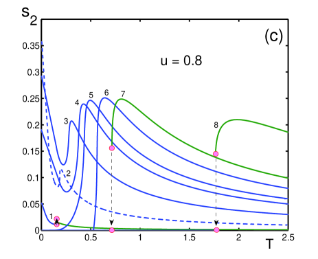
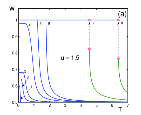
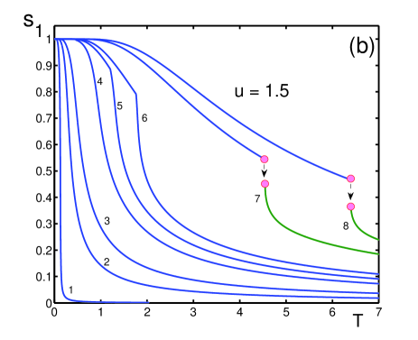
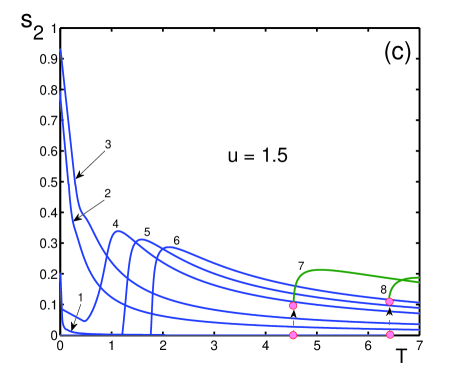
The most stable solution corresponds to the minimal of all those Gibbs potentials. The results of numerical calculations are presented in Figs. 1 to 5.

Depending on the value of the parameter $u$, it is possible to separate several regions with qualitatively different behavior. First of all, when $u\equiv 0$, mesoscopic fluctuations do not arise, as well as they are suppressed for very strong external field $h\rightarrow\infty$. Therefore, we shall concentrate our attention on the region of $u>0$ and not too large external field $h$. We analyze the behavior of the order parameters $w$, $s_{1}$, and $s_{2}$ as functions of $T$ for varying $h$.

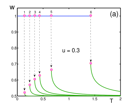
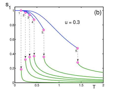
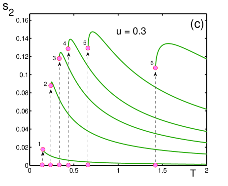
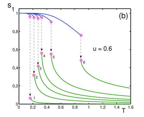
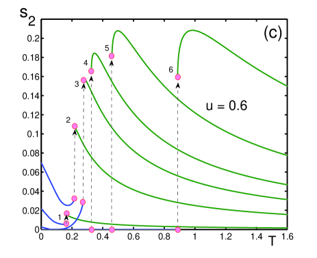
In the region $0<u<0.5$, the occurrence of multiscale fluctuations leads to the appearance of first-order phase transitions. Figure 1 shows the order parameters $w,s_{1}$, and $s_{2}$ as functions of temperature $T$ for different values of the field $h$, at fixed $u=0.3$. At zero $T$, there are no mesoscopic fluctuations, but they arise for $T>0$.

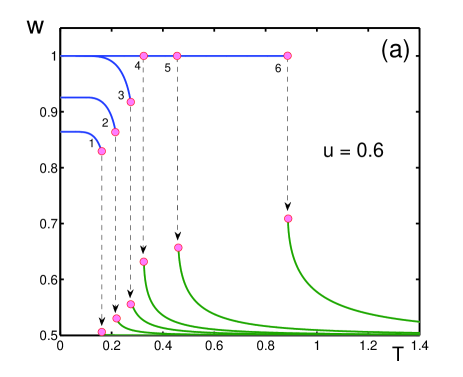
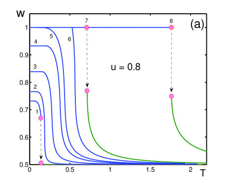
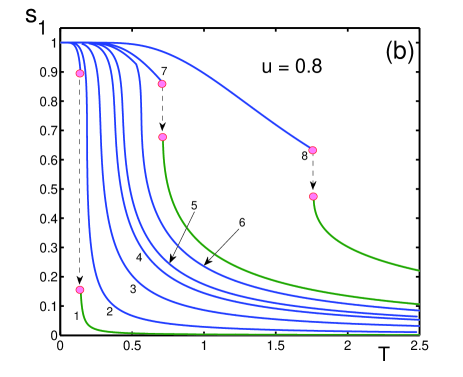
Larger values of the repulsion parameter $u$ make it possible, for some fields $h$, the appearance of mesoscopic fluctuations even at $T=0$. This is illustrated in Figs. 2 and 3. The difference of Fig. 3 from Fig. 2 is in the existence of a region of external fields, where, instead of a first-order phase transition, there occurs a sharp crossover.

When $u>1.5$, sharp crossovers are presented for low $T$, while the first-order transitions appear at higher $T$. This is shown in Fig. 4.

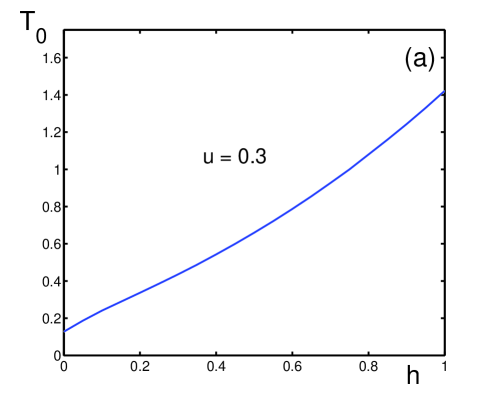
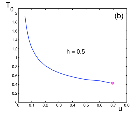
The first-order phase transition lines are presented in Fig. 5, as a function of $h$, at fixed $u$, and as a function of $u$, at given $h$. Increasing the external field $h$ shifts the phase transition point to the right, while increasing $u$ diminishes the transition temperature. When $u\rightarrow 0$, then the transition temperature tends to infinity, in agreement with the fact that at $u=0$, there are no mesoscopic fluctuations. For example, at $h=0.5$ and $u=0.001$, the transition temperature is $T_{0}=626$.

The general understanding is as follows. Taking into account the existence of mesoscopic multiscale fluctuations is crucially important. Their existence leads to the occurrence of first-order phase transitions or sharp crossovers between the strong-orbital coupling and weak-orbital coupling states of macromolecules. Increasing the intensity of noise, or temperature, results in the appearance by a jump of mesoscopic fluctuations, when the geometric weight of the strong-coupling phase, $w$, abruptly falls down. Respectively, the strong-coupling order parameter $s_{1}$ also falls down by a jump, while the weak-coupling order parameter $s_{2}$ suddenly increases. The point of such a phase transition depends on the values of the system parameters $u$ and $h$.

5 Classical Multiscale Fluctuations

As has been mentioned above, we have considered the case of multiscale fluctuations in a quantum macromolecular system. This has been done for generality, keeping in mind that many biological systems possess quantum properties. However, multiscale fluctuations can equally arise in classical systems. In order to show how they should be described in that case, we present below the approach for considering the statistics of multiscale fluctuations in the language of classical statistical mechanics.

Let us consider a system composed of $N$ atoms or molecules, enumerated with the index $i=1,2,\ldots,N$. The collections of all spatial variables and momenta are denoted through the sets

$$r^{N}\equiv\{{\bf r}_{1},{\bf r}_{2},\ldots,{\bf r}_{N}\}\;,\qquad p^{N}\equiv\{{\bf p}_{1},{\bf p}_{2},\ldots,{\bf p}_{N}\}\;,$$ (88)

respectively. The related differentials are abbreviated as

$$dr^{N}\equiv\prod_{i=1}^{N}d{\bf r}_{i}\;,\qquad dp^{N}\equiv\prod_{i=1}^{N}d{\bf p}_{i}\;.$$

Kinetic energy of $N$ atoms is

$$K(p^{N})=\sum_{i=1}^{N}\frac{{\bf p}_{i}^{2}}{2m}\;.$$ (89)

And the potential energy writes as

$$\frac{1}{2}\;\Phi\left(r^{N}\right)=\frac{1}{2}\sum_{i\neq j}^{N}\Phi({\bf r}_{i}-{\bf r}_{j})\;.$$ (90)

The overall consideration is the same as in Sec. 2. Under a fixed spatial separation of phases, we have the Hamiltonian $H(\xi)=\sum_{\nu}H_{\nu}$, with the terms

$$H_{\nu}\left(\xi,r^{N},p^{N}\right)=\sum_{i=1}^{N}\xi_{\nu i}\;\frac{{\bf p}_{i}^{2}}{2m}+\frac{1}{2}\sum_{i\neq j}^{N}\xi_{\nu i}\xi_{\nu j}\Phi({\bf r}_{i}-{\bf r}_{j})\;,$$ (91)

where $\xi_{\nu i}\equiv\xi_{\nu}({\bf r}_{i})$ is the manifold indicator defined in Eq. (14). The latter is normalized as

$$\sum_{i=1}^{N}\xi_{\nu}({\bf r}_{i})=N_{\nu}\;,$$ (92)

with $N_{\nu}$ being the number of atoms composing the $\nu$-th phase. Accomplishing the averaging over the configurations of multiscale fluctuations, according to Sec. 2, we get the effective Hamiltonian, similar to Eq. (26), with the terms

$$H_{\nu}\left(r^{N},p^{N}\right)=w_{\nu}K(p^{N})+\frac{w_{\nu}^{2}}{2}\;\Phi(r^{N})\;,$$ (93)

where the phase weights are

$$w_{\nu}=\frac{N_{\nu}}{N}\;.$$ (94)

The canonical partition function for a heterophase system with multiscale fluctuations reads as

$$Z(T,V,N)=\prod_{\nu}Z_{\nu}(T,V,N)\;,\qquad Z_{\nu}(T,V,N)=\int_{\cal{G}}\exp\left\{-\beta H_{\nu}(r^{N},p^{N})\right\}\;\frac{dr^{N}dp^{N}}{N!(2\pi)^{3N}}\;,$$ (95)

where the integration is over the phase volume

$${\cal{G}}\equiv\mathbb{V}^{N}\times\mathbb{R}^{3N}=\{{\bf r}_{i}\in\mathbb{V},\;{\bf p}_{i}\in\mathbb{R}^{3}:\;i=1,2,\ldots,N\}\;.$$ (96)

Integrating out the momenta, we have

$$Z_{\nu}(T,V,N)=\left(\frac{mT}{2\pi w_{\nu}}\right)^{3N/2}\int_{\mathbb{V}^{N}}\exp\left\{-\;\frac{w_{\nu}^{2}}{2T}\;\Phi(r^{N})\right\}\;\frac{dr^{N}}{N!}\;.$$ (97)

Having defined the system partition function, it is straightforward to calculate the desired thermodynamic characteristics.

6 Density and Size Fluctuations

To be more specific, let us consider the case when multiscale fluctuations correspond to mesoscopic density fluctuations, so that, at each moment of time, the system consists of randomly distributed mesoscopic regions having density $\rho_{1}$, which are intermixed with the regions of density $\rho_{2}$. And let, for concreteness, the first phase be more dense than the second one:

$$\rho_{1}>\rho_{2}\;.$$ (98)

The densities $\rho_{\nu}$ play here the role of the order parameters distinguishing different phases, the dense phase ($\nu=1$) and the rarified phase ($\nu=2$).

It is clear that, when the majority of $N$ atoms are in the dense phase, the system volume $V_{1}\sim N/\rho_{1}$ is smaller than the volume $V_{2}\sim N/\rho_{2}$, when almost all atoms are in the rarified phase. The transition from the smaller volume $V_{1}$ to the larger volume $V_{2}$ implies the system swelling, while the opposite transition from the larger volume $V_{2}$ to the smaller volume $V_{1}$ describes the system squeezing.

Since in this consideration, the system volume is not conserved, it is necessary to employ the isobaric ensemble, for which the system partition function is a function of temperature $T$, pressure $P$, and the total number of atoms $N$. For the heterophase system, the isobaric partition function is

$$Q(T,P,N)=\prod_{\nu}Q_{\nu}(T,P,N)\;,\qquad Q_{\nu}(T,P,N)=\int_{0}^{\infty}e^{-\beta PV}Z_{\nu}(T,V,N)\;dV\;.$$ (99)

So that the Gibbs potential is the sum

$$G(T,P,N)=\sum_{\nu}G_{\nu}(T,P,N)$$ (100)

of the terms

$$G_{\nu}(T,P,N)=-T\ln Q_{\nu}(T,P,N)\;.$$ (101)

The phase weights are defined by minimizing the Gibbs potential over $w_{\nu}$, under the normalization condition $w_{1}+w_{2}=1$. Setting $w\equiv w_{1},w_{2}=1-w$ makes it possible to write the minimization condition as

$$\frac{\partial G}{\partial w}=0\;,\qquad G=G(T,P,N)\;.$$ (102)

The observable quantities can be represented as the averages over the distribution function

$$f_{\nu}(r^{N},p^{N},V)=\frac{1}{Q_{\nu}}\;\exp\{-\beta(H_{\nu}+PV)\}\;,$$

where the Hamiltonian $H_{\nu}=H_{\nu}(r^{N},p^{N})$ is given in Eq. (91). This distribution is normalized by the condition

$$\int_{0}^{\infty}\left\{\int_{\cal{G}}f_{\nu}(r^{N},p^{N},V)\;\frac{dr^{N}dp^{N}}{N!(2\pi)^{3N}}\right\}\;dV=1\;.$$

The average of a function $A_{\nu}=A_{\nu}(r^{N},p^{N})$ is defined as

$$\langle A_{\nu}\rangle=\int_{0}^{\infty}\left\{\int_{\cal{G}}A_{\nu}(r^{N},p^{N})f_{\nu}(r^{N},p^{N},V)\;\frac{dr^{N}dp^{N}}{N!(2\pi)^{3N}}\right\}\;dV\;.$$

For example, the mean kinetic energy of the $\nu$-th phase, takes the form

$$K_{\nu}=\int_{0}^{\infty}\left\{\int_{\cal{G}}K_{\nu}(p^{N})f_{\nu}(r^{N},p^{N},V)\;\frac{dr^{N}dp^{N}}{N!(2\pi)^{3N}}\right\}\;dV\;,$$

which can be reduced to

$$K_{\nu}=\frac{3TN}{2w_{\nu}}\;.$$

And the mean potential energy of the $\nu$-th phase is $(1/2)\Phi_{\nu}$, where

$$\Phi_{\nu}=\int_{0}^{\infty}\left\{\int_{\cal{G}}\Phi_{\nu}(p^{N})f_{\nu}(r^{N},p^{N},V)\;\frac{dr^{N}dp^{N}}{N!(2\pi)^{3N}}\right\}\;dV\;.$$

Minimizing the Gibbs potential (98), according to condition (100), with taking into account that

$$\frac{\partial G}{\partial w_{\nu}}=\left\langle\frac{\partial H_{\nu}}{\partial w_{\nu}}\right\rangle\;,$$

we find the equation for the weight of the dense phase

$$w=\frac{\Phi_{2}+K_{2}-K_{1}}{\Phi_{1}+\Phi_{2}}\;,$$

which is similar to Eq. (42).

The total system volume is defined through the derivative

$$V(T,P,N)=\frac{\partial G}{\partial P}=V_{1}+V_{2}\;,$$

with the partial volumes

$$V_{\nu}=\frac{\partial G_{\nu}}{\partial P}=V_{\nu}(T,P,N)\;.$$

In this way, we find the densities of the competing phases

$$\rho_{\nu}\equiv\frac{N_{\nu}}{V_{\nu}}=w_{\nu}N\left(\frac{\partial G_{\nu}}{\partial P}\right)^{-1}\;.$$

At low temperature, when $w_{1}>w_{2}$, almost all atoms are in the dense phase, so that $N\sim N_{1}$ and $V\sim V_{1}$, though the occurrence of the multiscale density fluctuations results in the existence of the regions of the rarified phase. Rising temperature leads to the intensification of the mesoscopic density fluctuations and to the increase of the weight $w_{2}$. Then, these multiscale density fluctuations provoke the transition to the state, where $w_{2}>w_{1}$, so that the system volume increases, becoming close to $V_{2}$, though a small admixture of the dense-phase fluctuations can remain. Such a swelling transition is illustrated by Fig. 6.

7 Conclusion

Macromolecular systems are investigated experiencing, in addition to fast atomic fluctuations, slow multiscale fluctuations corresponding to the coherent motion of groups of many atoms. In the process of this motion, the system symmetry can be locally broken or restored in a spontaneous way⁶⁵. When the experimental observation time of the system is sufficiently long, being much longer than the atomic correlation time, one does not need to study the detailed dynamics of all atoms. In such experiments, one observes the smoothed picture averaged over many mesoscopic multiscale fluctuations. Then what one has to know is the statistics of multiscale fluctuations, that is, the average influence of these fluctuations on the values of observable quantities.

A method is suggested for treating the statistical influence of multiscale fluctuations on observables. The method is based on the Gibbs theory of quasi-equilibrium systems, with averaging over the ensemble of multiscale fluctuations. As a result, one comes to an effective statistical system with renormalized interactions and with the influence of the multiscale fluctuations incorporated into geometric weights of competing phases.

The method is illustrated for a macromolecular system exhibiting two possible states differing by the strength of coupling between atomic orbitals. Multiscale fluctuations in space and time occur between these two states, of weak-orbital and strong-orbital coupling. The order parameters of the system are calculated. The presence of mesoscopic fluctuations is shown to lead to sharp phase transitions between the phases of orbital weak-coupling and strong-coupling. Such phase transitions can be accompanied by an essential swelling or squeezing of macromolecules.

As is shown, the existence of mesoscopic multiscale fluctuations may result in drastic changes in the properties of macromolecules. When varying temperature, or other thermodynamic parameters, macromolecules can change their properties not gradually, but in a sharp phase transition. This is necessary to take into account in analyzing the behavior of macromolecules under the variation of external conditions. For example, considering the problem of the origin of life on Earth, one assumes that life appeared after the primordial ocean was cooled down ^66-70. In this respect, one often argues that it looks strange that biomolecules have arisen so suddenly, while the process of cooling was gradual. However, this does not seem strange if we take into account mesoscopic multiscale fluctuations. As is shown above, under a slow gradual cooling, the properties of macromolecules can change by an abrupt jump. It is, probably, the occurrence of mesocopic fluctuations that facilitated the spontaneous generation of life on Earth.

The aim of the present paper has been threefold. First, to develop a general approach allowing one to describe the statistics of multiscale fluctuations in macromolecules, without the need of studying their dynamics. Second, to demonstrate the use of the approach by a model that, though being simple, nevertheless exhibits rather rich properties, with phase transitions provoked by the multiscale fluctuations. Third, to emphasize that the approach is equally applicable to quantum as well as to classical systems. We have limited ourselves by these principal problems. Applications to particular biomolecules, having complicated structure, require separate investigations, with extensive computer calculations that are out of the scope of the present paper and are planned for future research.

Acknowledgement

The authors acknowledge financial support from the Russian Foundation of Basic Research.

References

(1) Miao, Y.; Ortoleva, P.J. J. Chem. Phys. 2006, 125, 214901.

(2) Pankavich, S.,; Mao, Y.; Ortoleva, J.; Shreif, Z.; Ortoleva, P. J. Chem. Phys. 2008, 128, 234908.

(3) Pankavich, S.; Shreif, Z.; Ortoleva, P. Physica A 2008, 387, 4053-4069.

(4) Mao, Y.; Johnson, J.E.; Ortoleva, P.J. J. Phys. Chem. B 2010, 114, 11181-11195.

(5) Pankavich, S.; Ortoleva, P. J. Math. Phys. 2010, 51, 063303.

(6) Singharoy, A.; Cheluvaraja, S.; Ortoleva, P. J. Chem. Phys. 2011, 134, 044104.

(7) Shreif, Z.; Ortoleva, P. J. Chem. Phys. 2011, 134, 104106.

(8) Wernsdorfer, W. Adv. Chem. Phys. 2001, 118, 99-190.

(9) Ferré, J. Topics Appl. Phys. 2002, 83, 127-168.

(10) Yukalov, V.I.; Yukalova, E.P. Phys. Part. Nucl. 2004, 35, 348-382.

(11) Liu, J.P.; Fullerton, E.; Gutfleisch, O.; Sellmyer, D.J., Eds. Nanoscale Magnetic Materials and Applications; Springer: Berlin, 2009.

(12) Chakraborty, T. Quantum Dots; North Holland: Amsterdam, 1999.

(13) Leatherdale, C.A.; Woo, W.K.; Mikulec, F.V.; Bawendi, M.G. J. Phys. Chem. B 2002, 106, 7619 7622.

(14) Lieb, E.H.; Seiringer, R.; Solovej, J.P.; Yngvason, J. The Mathematics of the Bose Gas and Its Condensation; Birkhauser: Basel, 2005.

(15) Letokhov, V. Laser Control of Atoms and Molecules; Oxford University: New York, 2007.

(16) Pethik C.J.; Smith, H. Bose-Einstein Condensation in Dilute Gases; Cambridge University: Cambridge, 2008.

(17) Courteille, P.W.; Bagnato, V.S.; Yukalov, V.I. Laser Phys. 2001, 11, 659-800.

(18) Andersen, J.O. Rev. Mod. Phys. 2004, 76, 599- 639.

(19) Yukalov, V.I. Laser Phys. Lett. 2004, 1, 435-461.

(20) Bongs, K.; Sengstock, K. Rep. Prog. Phys. 2004, 67, 907-963.

(21) Yukalov, V.I.; Girardeau, M.D. Laser Phys. Lett. 2005, 2, 375-382.

(22) Posazhennikova, A. Rev. Mod. Phys. 2006, 78, 1111-1134.

(23) Yukalov, V.I. Laser Phys. Lett. 2007, 4, 632-647.

(24) Proukakis, N.P.; Jackson, B. J. Phys. B 2008, 41, 203002.

(25) Yurovsky, V.A.; Olshanii, M.; Weiss, D.S. Adv. At. Mol. Opt. Phys. 2008, 55, 61-138.

(26) Ketterle, W.; Zwierlein, M.W. Riv. Nuovo Cimento 2008, 31, 247-422.

(27) Moseley, C.; Fialko, O.; Ziegler, K. Ann. Phys. (Berlin) 2008, 17, 561-608.

(28) Yukalov, V.I. Laser Phys. 2009, 19, 1-110.

(29) Yukalov, V.I. Phys. Part. Nucl. 2011, 42, 460-513.

(30) Lee, S.W.; Mao, C.; Flynn, C.E.; Belcher, A.M. Science 2002, 296, 892-895.

(31) Frenkel, J. Kinetic Theory of Liquids; Clarendon: Oxford, 1946.

(32) Fisher, M.E. Nature of Critical Points; Colorado University: Boulder, 1965.

(33) Fisher, M.E. Rep. Prog. Phys. 1967, 30, 615-730.

(34) Khait, Y.L. Phys. Rep. 1983, 99, 237-340.

(35) Khait, Y.L. Atomic Diffusion in Solids; Scitec: Z rich, 1997.

(36) Engel, G.S.; Calhoun, T.S.; Read, E.L.; Ahn, T.K.; Mancal, T.; Cheng, Y.C.; Blankenship, R.E.; Fleming, G.R. Nature 2007, 446, 782-786.

(37) Collini, E.; Wong, C.Y.; Wilk, K.E.; Curni, P.M.; Bruner, P.; Scholes, G.D. Nature 2010, 463, 644-647.

(38) Panitchayangkoon, G.; Hayes, D.; Fransted, K.A.; Caram, J.R.; Harel, E.; Wen, J.; Blankenship, R.E.; Engel, G.S. Proc. Natl. Acad. Sci. USA 2010, 107, 12766-12770.

(39) Gauger, E.M.; Rieper, E.; Morton, J.J.; Benjamin, S.C.; Vedral, V. Phys. Rev. Lett. 2011, 106, 040503.

(40) Franco, M.I.; Turin, L.; Mershin, A.; Skoulakis, E.M. Proc. Natl. Acad. Sci. USA 2011, 108, 3797-3802.

(41) Yukalov, V.I., Physica A 1986 136, 575-587.

(42) Yukalov, V.I. Physica A 1987, 141, 352-374.

(43) Yukalov, V.I. Phys. Rep. 1991, 208, 395-489.

(44) Coleman, A.J.; Yukalov, V.I. Reduced Density Matrices; Springer: Berlin, 2001.

(45) Yukalov, V.I. Physica A 2002, 310, 413-434.

(46) Gibbs, J.W. Collected Works; Longmans: New York, 1928.

(47) Gibbs, J.W. Elementary Priciples in Statistical Mechanics; Cambridge University: Cambridge, 2010.

(48) Ono, S.; Kondo, S. Molecular Theory of Surface Tension in Liquids; Springer: Berlin, 1960.

(49) Krotov, V.V.; Rusanov, A.I. Physicochemical Hydrodynamics of Capillary Systems; World Scientific: Singapore, 1999.

(50) Terletsky, Y.P. Statistical Physics; Higher School: Moscow, 1973.

(51) Bogolubov, N.N. Lectures on Quantum Statistics, Vol. 2; Gordon and Breach: New York, 1970.

(52) Yukalov, V.I. Phys. Rev. B 1985, 32, 436-446.

(53) Yukalov, V.I. Phys. Lett. A 1987, 125, 95-100.

(54) Yukalov, V.I.; Yukalova, E.P. Int. J. Mod. Phys. B 2001, 15, 2433-2453.

(55) Boky, M.A.; Kudryavtsev, I.K.; Yukalov, V.I. Solid State Commun. 1987, 63, 731-735.

(56) Boky, M.A.; Yukalov, V.I. in Problems of Statistical Mechanics, Bogolubov, N.N. Ed., Vol. 1, p. 170-176; JINR: Dubna, 1984.

(57) Yukalov, V.I. Int. J. Mod. Phys. B 1992, 6, 91-107.

(58) Coleman, A.J.; Yukalova, E.P.; Yukalov, V.I. Physica C, 1995, 243, 76-92.

(59) Yukalov, V.I.; Yukalova, E.P. Phys. Rev. B 2004, 70, 224516.

(60) Yukalov, V.I.; Yukalova, E.P. Physica A 1997, 243, 382-414.

(61) Yukalov, V.I.; Yukalova, E.P. Phys. Part. Nucl. 1997, 28, 37-65.

(62) Ter Haar, D. Lectures on Selected Topics in Statistical Mechanics; Pergamon: Oxford, 1977.

(63) Kirkwood, J.G. Quantum Statistics and Cooperative Phenomena; Gordon and Breach: New York, 1965.

(64) Mitin, A.V.; Hirsch, G. J. Math. Chem. 1994, 15, 109-113.

(65) Yukalov, V.I. Phys. Lett. A 1981, 85, 68-71.

(66) Oparin, A.I. Origin of Life; Dover: New York, 1953.

(67) Bernal, J.D. Origins of Life; Wiedenfeld and Nicholson: London, 1969.

(68) Dyson, F. Origins of Life; Cambridge University: Cambridge, 1985.

(69) Bryson, B. A Short History of Nearly Everything; Black Swan: London, 2004.

(70) Egel, R.; Lankenau, D.H.; Mulkidjanian, A.Y. Origins of Life: The Primal Self-Organization; Springer: Berlin, 2011.

Figure Captions

Fig. 1. Macromolecule order parameters: (a) geometric weight of the strong-coupling phase $w$; (b) strong-coupling phase order parameter $s_{1}$; (c) weak-coupling phase order parameter $s_{2}$. Dependence on dimensionless temperature is shown for the repulsion parameter $u=0.3$ and varying strength of external field: (1) $h=0.01$; (2) $h=0.1$; (3) $h=0.2$; (4) $h=0.3$; (5) $h=0.5$; (6) $h=1$. The corresponding first-order transition temperatures are: (1) $T_{0}=0.145$; (2) $T_{0}=0.241$; (3) $T_{0}=0.336$; (4) $T_{0}=0.436$; (5) $T_{0}=0.660$; (6) $T_{0}=1.422$.

Fig. 2. Macromolecule order parameters: (a) $w$; (b) $s_{1}$; (c) $s_{2}$. Dependence on dimensionless temperature is shown for the repulsion parameter $u=0.6$ and varying strength of external field: (1) $h=0.01$; (2) $h=0.1$; (3) $h=0.2$; (4) $h=0.3$; (5) $h=0.5$; (6) $h=1$. The corresponding transition temperatures are: (1) $T_{0}=0.164$; (2) $T_{0}=0.217$; (3) $T_{0}=0.276$; (4) $T_{0}=0.326$; (5) $T_{0}=0.460$; (6) $T_{0}=0.877$.

Fig. 3. Macromolecule order parameters: (a) $w$; (b) $s_{1}$; (c) $s_{2}$. Dependence on dimensionless temperature is shown for $u=0.8$ and varying external field: (1) $h=0.01$; (2) $h=0.1$; (3) $h=0.2$; (4) $h=0.3$; (5) $h=0.5$; (6) $h=0.8$; (7) $h=1$; (8) $h=2$. The first-order transition temperatures are: (1) $T_{0}=0.143$; (7) $T_{0}=0.715$; (8) $T_{0}=1.764$. For the values $0.01<h<1$, the transition is a sharp crossover.

Fig. 4. Macromolecule order parameters: (a) $w$; (b) $s_{1}$; (c) $s_{2}$. Dependence on dimensionless temperature is shown for $u=1.5$ and varying external field: (1) $h=0.01$; (2) $h=0.5$; (3) $h=1$; (4) $h=2$; (5) $h=2.5$; (6) $h=3$; (7) $h=5$; (8) $h=6$. The transition temperatures are: (7) $T_{0}=4.547$; (8) $T_{0}=6.4$. For the values $h<5$, the transition occurs as a sharp crossover.

Fig. 5. First-order transition temperature $T_{0}$: (a) as a function of $h$ at fixed $u=0.3$; (b) as a function of $u$ at fixed $h=0.5$.

Fig. 6. Qualitative illustration of the macromolecule swelling provoked by multiscale mesoscopic density fluctuations.

                 

Figure 1: Macromolecule order parameters: (a) geometric weight of the strong-coupling phase $w$; (b) strong-coupling phase order parameter $s_{1}$; (c) weak-coupling phase order parameter $s_{2}$. Dependence on dimensionless temperature is shown for the repulsion parameter $u=0.3$ and varying strength of external field: (1) $h=0.01$; (2) $h=0.1$; (3) $h=0.2$; (4) $h=0.3$; (5) $h=0.5$; (6) $h=1$. The corresponding first-order transition temperatures are: (1) $T_{0}=0.145$; (2) $T_{0}=0.241$; (3) $T_{0}=0.336$; (4) $T_{0}=0.436$; (5) $T_{0}=0.660$; (6) $T_{0}=1.422$.

                 

Figure 2: Macromolecule order parameters: (a) $w$; (b) $s_{1}$; (c) $s_{2}$. Dependence on dimensionless temperature is shown for the repulsion parameter $u=0.6$ and varying strength of external field: (1) $h=0.01$; (2) $h=0.1$; (3) $h=0.2$; (4) $h=0.3$; (5) $h=0.5$; (6) $h=1$. The corresponding transition temperatures are: (1) $T_{0}=0.164$; (2) $T_{0}=0.217$; (3) $T_{0}=0.276$; (4) $T_{0}=0.326$; (5) $T_{0}=0.460$; (6) $T_{0}=0.877$.

                 

Figure 3: Macromolecule order parameters: (a) $w$; (b) $s_{1}$; (c) $s_{2}$. Dependence on dimensionless temperature is shown for $u=0.8$ and varying external field: (1) $h=0.01$; (2) $h=0.1$; (3) $h=0.2$; (4) $h=0.3$; (5) $h=0.5$; (6) $h=0.8$; (7) $h=1$; (8) $h=2$. The first-order transition temperatures are: (1) $T_{0}=0.143$; (7) $T_{0}=0.715$; (8) $T_{0}=1.764$. For the values $0.01<h<1$, the transition is a sharp crossover.

                 

Figure 4: Macromolecule order parameters: (a) $w$; (b) $s_{1}$; (c) $s_{2}$. Dependence on dimensionless temperature is shown for $u=1.5$ and varying external field: (1) $h=0.01$; (2) $h=0.5$; (3) $h=1$; (4) $h=2$; (5) $h=2.5$; (6) $h=3$; (7) $h=5$; (8) $h=6$. The transition temperatures are: (7) $T_{0}=4.547$; (8) $T_{0}=6.4$. For the values $h<5$, the transition occurs as a sharp crossover.

                 

Figure 5: First-order transition temperature $T_{0}$: (a) as a function of $h$ at fixed $u=0.3$; (b) as a function of $u$ at fixed $h=0.5$.

Figure 6: Qualitative illustration of the macromolecule swelling provoked by multiscale mesoscopic density fluctuations.