Anomalous Diffusion and Long-range Correlations in the Score Evolution of the Game of Cricket

Abstract

We investigate the time evolution of the scores of the second most popular sport in world: the game of cricket. By analyzing the scores event-by-event of more than two thousand matches, we point out that the score dynamics is an anomalous diffusive process. Our analysis reveals that the variance of the process is described by a power-law dependence with a super-diffusive exponent, that the scores are statistically self-similar following a universal Gaussian distribution, and that there are long-range correlations in the score evolution. We employ a generalized Langevin equation with a power-law correlated noise that describe all the empirical findings very well. These observations suggest that competition among agents may be a mechanism leading to anomalous diffusion and long-range correlation.

Diffusive motion is ubiquitous in nature. It can represent how a drop of ink spreads in water, how living organisms such as fishes Skalski or bacteria Ishikawa move, how information travels over complex networks Iribarren , and many other phenomena. One of the most common fingerprints of usual diffusion is the way that particles or objects in question spread. The spreading can be measured as the variance of the positions of the particles after a certain period of time. For usual diffusion, the variance grows linearly in time. There are two hypothesis underlying this behavior. The first one is the absence of memory along the particle trajectory, that is, the actual position of the particle can be approximated by a function of its immediately previous position (Markovian hypothesis). The second one is the existence of a characteristic scale for the position increments. When these two assumptions hold, we can show that distribution of the positions will approach a Gaussian profile (Central Limit Theorem).

Naturally, there are situations in nature that do not fit these hypothesis and, consequently, deviations from the usual behavior appear. When this happens, researchers usually report on anomalous diffusion. A well understood case is when there is no characteristic length for the particle jumps. In this case, the variance is infinity and the distribution of the positions follows a Lévy distribution. Examples of Lévy processes include the animals movement during foraging Humphries , diffusion of ultracold atoms Sagi and systems out of thermal equilibrium Bardou . The situation is more complex when the diffusive process presents memory. We have many different manners of correlating the particle positions. Depending on this choice, diffusive properties such as the dependence of the variance in time can drastically change. In this context, a typical behavior for the variance is a power-law dependence with an exponent $\alpha$, where $\alpha<1$ corresponds to sub-diffusion and $\alpha>1$ to super-diffusion.

Several approaches have been proposed to investigate anomalous diffusion in general. Fractional diffusion equations Metzler , Fokker-Planck equations Trigger , and Langevin equations Lim are just a few examples of frameworks used to describe this phenomenon. However, there is a lack of empirical studies aiming to verify situations where these models can be applied and the possible mechanisms that lead to anomalous diffusion. There are a few exceptions, such as the work of Weber, Spakowitz and Theriot Weber where they showed that the motion of chromosomal loci of two bacterial species is sub-diffusive and anti-correlated, as well as the work of Lenz et al. Lenz where they investigated the role of predation in the motion of bumblebees during foraging.

In this work, we show that the evolution of the scores in the game of cricket can be understood as a diffusive process with scale-invariance properties, anomalous diffusion, and long-range correlations. All these findings are well described by a generalized Langevin equation with a power-law correlated noise. The results presented here suggest that competition among agents may be a mechanism leading to correlation and anomalous diffusion correlation. In the following, we present our dataset of scores of cricket matches, a diffusive interpretation for the evolution of these scores, a generalized Langevin equation for modeling the empirical findings, and finally, some concluding remarks.

The game of cricket is the second most popular sport in the world after soccer. It is a “bat-and-ball” game (similar to baseball) played between two teams of 11 players. There are three types of the game that differ in length. The “Twenty20” (T20) cricket is the shortest one lasting approximately $3$ hours, the “One Day International” (ODI) cricket lasts almost $8$ hours, and the “Test” cricket is the longest one taking up to five days to finish. The game involves one team batting (their innings) and scoring as many points (runs) as possible and setting up a target for the opponent team. The opponent team comes in to bat and tries to exceed the target. A team’s innings is terminated whenever it exceeds the quota of overs (six consecutive balls bowled in succession) or when the team lost 10 wickets (wooden stumps used as a target for the bowling). The maximum limit is $20$ overs for T20 cricket, $50$ overs for ODI cricket, and $200$ overs for Test cricket.

Figure 1: Evolution of the scores $S(t)$ for the different three types of cricket. To make the notation easier, we have denoted the event-by-event evolution as time evolution. The main difference between these types is the maximum length of game. The maximum length is 20 time steps for T20, 50 for ODI, and 200 for test. In panel (A) we plot the evolution of the scores of a hundred games selected at random from our database, and in panel (B) we show these evolution after removing the mean tendency of increase, that is, $S(t)-\langle S(t)\rangle$.

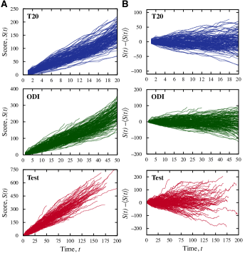
Surprisingly, the record of a game of cricket (score cards) includes not only the game outcome, but also the event-by-event evolution of the scores. We collect the information of scores per over for T20 ($2005-2011$), ODI ($2002-2011$), and Test cricket ($2002-2011$) from the cricinfo website Site . Using these data, we create 2144 time series of scores where the time $t$ represents a completed over. In Figure 1A, we show the temporal dependence of the scores $S(t)$ for one hundred games from the three different types of cricket selected at random from our database. We note the natural increasing tendency of the scores and also the erratic movement around the mean tendency. For better visualization of these fluctuations, we plot in Fig. 1B the scores after subtracting the mean tendency $\langle S(t)\rangle$ from $S(t)$.

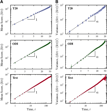
We start by investigating how the mean value of the scores depends on time (Fig. 2A). These plots reveal that the mean score $\langle S(t)\rangle$ grows linearly in time for the three types of the game. The only difference is in the rate of growth, which is $6.4\pm 1.0$ for T20, $3.9\pm 1.0$ for ODI, and $3.3\pm 1.0$ for Test. The different values show that the overall performance of teams are related to length of the game. In T20 cricket (which last $\sim 3$ hours) and in ODI cricket (which last $\sim 8$ hours), we have the highest rates indicating that the players work hard for scoring as many points as they can, while for Test cricket the players may prefer to save efforts, since Test matches are quite long.

Next, we characterize the spreading process by evaluating the variance of the scores as a function of time (Fig. 2B). We show the variance $\sigma^{2}(t)=\langle[S(t)-\langle S(t)\rangle]^{2}\rangle$ in a log-log plot, where we observe a non-linear increase of $\sigma^{2}(t)$. By least square fitting a linear model to these log-log data, we find a super-diffusive regime, that is, $\sigma^{2}(t)\propto t^{\alpha}$ with $\alpha\approx 1.3$ for the three types of cricket. This intriguing feature suggests that the competition within the game may drive the scores to spread faster than a regular Brownian motion.

Figure 2: The anomalous diffusion of the scores. (A) Mean value of the scores as a function of time, $\langle S(t)\rangle$, for the three types of the Cricket. The dashed lines are linear fits to each dataset. We find the mean values to grow linearly in time. (B) The spreading of the score trajectories measured as the variance $\sigma^{2}(t)=\langle[S(t)-\langle S(t)\rangle]^{2}\rangle$ versus time. The dashed lines are power-law fits to the variance, where we find the exponents $\alpha=1.32\pm 0.02$ for T20, $\alpha=1.31\pm 0.02$ for ODI, and $\alpha=1.30\pm 0.02$ for Test. Since $\alpha>1$, the diffusive process underlying the evolution of scores is super-diffusive. The error bars are $95\%$ confidence intervals obtained via bootstrapping Efron .

Figure 3: Scale invariance of the scores. (A) Evolution of the cumulative distribution function (CDF) for the three types of cricket and for different values of time $t$. Note that the distributions shift towards positive values of the score and that the width of the CDFs increases. (B) Scale invariance of the scores. We evaluate the CDF using the normalized scores $\xi(t)=\frac{S(t)-\langle S(t)\rangle}{\sigma(t)}$ where $\langle S(t)\rangle$ is the mean value of the scores and $\sigma(t)$ is the square root of the variance of the scores. Note that the good collapse of the distributions indicates that the scores present scaling properties, i.e., after normalization they follow the same universal distribution. In these plots, the continuous lines are the CDFs for each value of $t$ and the symbols are the averaged values of these CDFs. The error bars are $95\%$ confidence intervals obtained via bootstrapping Efron . We note further that these distributions are very close to a normalized Gaussian distribution (dashed lines). The insets show the p-values for the Pearson chi square test Greenwood as a function of time. The dashed line is the threshold $0.1$ for rejecting the Gaussian hypothesis. Note that the normality is rejected for small values of $t$ because of the discrete values of $S(t)$ and also the asymmetric initial condition of the diffusive process. After enough time, ($t\sim 90$), we can not reject the Gaussian hypothesis in the Test cricket.

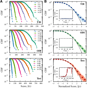
Another interesting question is whether the distribution of the scores is self-similar and whether these distributions follow a particular functional form. To answer this question, we calculate the cumulative distribution functions of the scores for each time step. Figure 3A shows these distributions for several values of $t$ and for the three types of cricket. We note the shift of the distributions towards positive values and the increase in the distribution width. Moreover, these semi-log plots indicates that the distributions are close to normal distributions.

To check the normality and self-similarity, we evaluate the distribution of the normalized scores $\xi(t)=\frac{S(t)-\langle S(t)\rangle}{\sigma(t)}$, where $\langle S(t)\rangle$ is the mean value of the score and $\sigma(t)$ is the standard-deviation. As shown in Fig. 3B, the distributions exhibit a good collapse and a profile that is very close to Gaussian distribution. These results are also supported by the insets of Fig. 3B, where we plot the p-values for the Pearson chi square test as a function of time. We note that the normality is rejected for small values of $t\lesssim 90$ due to the discrete nature of $S(t)$ and also the asymmetry in the score system. After enough time ($t\sim 90$), the p-values are larger than $0.1$ and we can not reject the Gaussian hypothesis in the Test cricket.

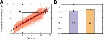
We now focus on correlation analysis to answer whether the scores evolution is a Markovian process. To investigate this hypothesis, we select all games from the Test cricket that are longer than 120 time steps, totaling 431 games. For this subset, we calculate the time series of the scores increments $\Delta S(t)=S(t+1)-S(t)$. Next, we employ detrended fluctuation analysis (DFA) to obtain the Hurst exponent $h$. DFA Peng ; Kantelhardt consists of four steps: $i)$ We first define the profile $Y(i)=\sum_{k=1}^{i}\Delta S(t)-\langle\Delta S(t)\rangle\,.$ $ii)$ Next, we cut $Y(i)$ into $N_{n}=N/n$ non-overlapping segments of size $n$, where $N$ is the length of the series. $iii)$ For each segment, a local polynomial trend (here we have used a linear function) is calculated and subtracted from $Y(i)$, defining $Y_{n}(i)=Y(i)-p_{\nu}(i)$, where $p_{\nu}(i)$ represents the local trend in the $\nu$-th segment. $iv)$ Finally, we evaluate the root-mean-square fluctuation function $F(n)=[\frac{1}{N_{n}}\sum_{\nu=1}^{N_{n}}\langle Y_{n}(i)^{2}\rangle_{\nu}]^{1/2}\,,$ where $\langle Y_{n}(i)^{2}\rangle_{\nu}$ is mean square value of $Y_{n}(i)$ over the data in the $\nu$-th segment. For self-similar time series, the fluctuation function $F(n)$ displays a power-law dependence on the time scale $n$, that is, $F(n)\sim n^{h}$, where $h$ is the Hurst exponent. Intriguingly, we find that the Hurst exponent does not depend on game and that it has a mean value equal to $h=0.63\pm 0.01$ (Fig. 4A). This result shows that there is long-range memory in the score evolution, and therefore it is a non-Markovian process. Moreover, the value of $h>0.5$ indicates the existence of a persistence behavior in the scores increments, that is, positive values are followed by positive values and negative values are followed by negative values much more frequently than by chance.

All the previous empirical findings claim for model. To address this question, we consider the following generalized Langevin equation for describing the score evolution of the Test cricket,

$$\frac{d^{2}S(t)}{dt^{2}}+\int_{0}^{t}\lambda(t-\tau)\frac{dS(\tau)}{d\tau}d\tau+K=\xi(t)\,.$$

Here, $\lambda(t-\tau)$ is the retarded effect of the frictional force, $K$ is a drift constant, and $\xi(t)$ represents a Gaussian stochastic force. Because we know that long-range correlations are present in our system, we consider that $\xi(t)$ is also power-law correlated, that is, $\langle\xi(0)\xi(t)\rangle\sim t^{-\alpha}$. We also assume $\lambda(t)\propto\langle\xi(0)\xi(t)\rangle$ in order to satisfy the fluctuation-dissipation theorem Kubo . This equation was presented in Refs. Lim ; Wang ; Wang2 for $K=0$ and it can be solved by using Laplace transform. Indeed, after some calculations, we can show that the mean score is linear in time $\langle S(t)\rangle\sim t$, that the variance obeys a power-law relationship $\langle[S(t)-\langle S(t)\rangle]^{2}\rangle\sim t^{-\alpha}$, and the distribution of the scores is Gaussian. Remarkably, these are exactly the same features that our empirical data present (see Figs. 2 and 3).

Furthermore, we calculate the auto-correlation function of the score “velocity” $\langle V(0)V(t)\rangle\sim t^{\alpha-2}$, where $V(t)=dS(t)/dt$ and $\alpha\neq 1$. Note that this derivative corresponds to the score increments $\Delta S(t)=S(t+1)-S(t)$ in the discrete case. Thus, the Langevin equation also predicts the existence of long-range memory in the score increments. We can check this prediction by observing that the power-law exponent of auto-correlation function is related to the Hurst exponent Kantelhardt , which consequently leads to a relationship between the Hurst and the diffusive exponent $\alpha=2h$. Figure 4B shows a bar plot that compares the value of $2h$ (left bar) with the value of $\alpha$ (right bar) for the Test cricket. We note that these values are close to each other and that there exists overlapping between the confidence intervals. Therefore, the relationship $\alpha=2h$ applies.

Figure 4: Long-range correlations in the scores. (A) Detrended fluctuation analysis of score increments $\Delta S(t)=S(t+1)-S(t)$. We show the fluctuation functions $F(n)$ versus the scale $n$ (continuous lines) for all games of the Test cricket that are longer than $120$ units of time (431 games). Note that $F(n)$ follows a power-law, where the exponent $h$ is the Hurst exponent. We estimate the mean value of Hurst exponent to be $h=0.63\pm 0.01$, and the dashed line is a power-law with this exponent. We find the average value of Pearson linear correlation coefficient equal to $0.89\pm 0.02$, which enhances the quality of the power-law relationships. The symbols represent the average values of the fluctuation functions and the error bars are standard errors of the means. (B) Comparison of the model prediction, that is, $\alpha=2h$ for the Test cricket. The left bar shows the empirical value of $2h$ and the right bar shows the value of $\alpha$. The error bars are $95\%$ confidence intervals and the horizontal line is the upper limit of the confidence interval for $2h$. We note the existence of overlapping in the confidence intervals, indicating that the relation $\alpha=2h$ holds.

In summary, we have studied the score evolution of cricket games as a diffusive process. Our analysis reveals that the mean score grows linearly in time, while the variance of the scores has a power-law dependence in time with a super-diffusive exponent. We show that the scores are statistically self-similar and follow a universal distribution approximated by a Gaussian. By using DFA, we point out that this diffusive process is non-Markovian since the scores increments are long-range correlated. It is worth to note that the persistent long-range memory present in the diffusive process can be related the “hot hand” phenomenon in sports. Since the seminal work of Gilovich et al. Gilovich there has been a historical debate on whether “success breeds success” or “failure breeds failure” in the scoring process of many sports Yaari ; Yaari2 . Here, the long-range persistent behavior in the score evolution not only indicates the existence of this phenomenon in cricket, but also suggests that this phenomenon can act over a very long temporal scale. Because of the long-range memory, we proposed to model the empirical findings using a generalized Langevin equation driven by a power-law correlated stochastic force. The correlation in the noise term induces the faster-than-regular spreading of the diffusive process and also gives rise to correlations in the score increments. The results of this model show that there is a simple relation between the diffusive exponent $\alpha$ and the Hurst exponent $h$, which we have verified to hold in the empirical data. We are optimistic that the discussion presented may be applied to other sports, where new analysis can reveal more complex diffusive patterns to be compared with the increasing number of theoretical results on anomalous diffusion.