RegPT: Direct and fast calculation of regularized cosmological power spectrum at two-loop order

Abstract

We present a specific prescription for the calculation of cosmological power spectra, exploited here at two-loop order in perturbation theory (PT), based on the multi-point propagator expansion. In this approach power spectra are constructed from the regularized expressions of the propagators that reproduce both the resummed behavior in the high-$k$ limit and the standard PT results at low-$k$. With the help of $N$-body simulations, we show that such a construction gives robust and accurate predictions for both the density power spectrum and the correlation function at percent-level in the weakly non-linear regime. We then present an algorithm that allows accelerated evaluations of all the required diagrams by reducing the computational tasks to one-dimensional integrals. This is achieved by means of pre-computed kernel sets defined for appropriately chosen fiducial models. The computational time for two-loop results is then reduced from a few minutes, with the direct method, to a few seconds with the fast one. The robustness and applicability of this method are tested against the power spectrum cosmic emulator from which a wide variety of cosmological models can be explored. The fortran program with which direct and fast calculations of power spectra can be done, RegPT, is publicly released as part of this paper.

I Introduction

Since recombination, the large-scale structure of the Universe has evolved dominantly under the influence of both the cosmic expansion and the force of gravity acting on a pressure-less fluid. The statistical nature of its spatial clustering is therefore expected to bring valuable cosmological information about the dynamics of the cosmic expansion and structure formation. Of particular importance is the measurement of baryon acoustic oscillations (BAOs) imprinted on the power spectrum or two-point correlation function (e.g., Eisenstein et al. (2005); Percival et al. (2010); Blake et al. (2011a); Seo et al. (2012); Anderson et al. (2012)) from which one can precisely determine the cosmological distance to the high-redshift universe, and henceforth clarify the nature of late-time cosmic acceleration (e.g., Seo and Eisenstein (2003); Blake and Glazebrook (2003); Glazebrook and Blake (2005); Shoji et al. (2009); Padmanabhan and White (2008)). Precious information regarding the growth of structure are and will also be obtained from redshift-space distortions (e.g., Linder (2008); Guzzo et al. (2008); Yamamoto et al. (2008); Song and Percival (2009); Blake et al. (2011b)) and weak lensing measurements (see Van Waerbeke et al. (2000); Fu et al. (2008) and review papers Bartelmann and Schneider (2001); Van Waerbeke and Mellier (2003)) at scales ranging to the linear or quasi-linear to the non-linear regimes. This could be captured with unprecedented details with the ongoing and future surveys, thanks to their redshift depth and large angular area, such as the Sloan Digital Sky Survey III, the WiggleZ survey, the Subaru Measurement of Imaging and Redsfhits, the Dark Energy Survey, the BigBOSS project, the Physics of the Accelerating Universe collaboration and the ESA/Euclid survey .

With the advent of such wealth of observations, there is therefore a growing interest in the development of theoretical tools to accurately compute the statistical quantities of the large-scale structure. At decreasing redshift and scale, the evolution of the large-scale structure however deviates significantly from the linear theory prediction and non-linear gravitational clustering effects have to be taken into account. While $N$-body simulations can be relied upon in specific cases, because of the range of scales to be covered and the variety of models to explore, they should be complemented by analytical investigations that aim at computing the statistical properties of the large-scale structure from first principles, henceforth extending the validity range of linear calculations. It is to be noted that even at the scale of BAOs, linear calculations and one-loop standard PT corrections perform poorly (see e.g., Crocce and Scoccimarro (2006a); Carlson et al. (2009); Taruya et al. (2009)) asking for more advanced PT calculations. The improvement of perturbation theory is thus a critical issue for the scientific exploitation of the coming surveys. Various resummation schemes have been proposed in Refs. Crocce and Scoccimarro (2006a, b); Crocce and Scoccimarro (2008); Matsubara (2008a, b); McDonald (2007); Izumi and Soda (2007); Taruya and Hiramatsu (2008); Taruya et al. (2009); Pietroni (2008); Matarrese and Pietroni (2007); Valageas (2004, 2007) that aim at improving upon standard schemes. The aim of this paper is not to compare them but to propose, and test, a specific scheme that can be used routinely in practice.

In this paper, we are particularly interested in one of the resummation treatments, advocated in Ref. Bernardeau et al. (2008). In this approach, the standard PT expansion is re-organized by introducing the multi-point propagators. These are the ensemble average of the infinitesimal variation of the cosmic fields with respect to the initial conditions. A key property shown in the previous reference is that all the statistical quantities such as power spectra and bispectra can be re-constructed by an expansion series written solely in terms of the multi-point propagators. This is referred to as the multi-point propagator expansion or $\Gamma$-expansion. The advantage of this approach is that the non-perturbative properties, which can be obtained in standard PT by summing up infinite series of PT expansions, are whole encapsulated in the multi-point propagators, including the effect of vertex renormalization. Furthermore, the $\Gamma$-expansion has been found to be valid not only for Gaussian initial conditions, but also for non-Gaussian ones Bernardeau et al. (2010). The construction of accurate calculation scheme for power spectra and bispectra can then be split in pieces that can be tested separately.

The second key property that leads us to consider such objects is that their global shape, e.g. their whole $k$-dependence, can be computed in a perturbation theory context and compared to $N$-body results thanks to the high-$k$ exponential damping tail they all exhibit Bernardeau et al. (2008); Bernardeau et al. (2012a). All these properties make the multi-point propagators the most important building blocks in the $\Gamma$-expansion and the focus of our modeling efforts. In the following we will in particular make full use of the novel regularization scheme proposed in Ref. Bernardeau et al. (2012b) that allows to consistently interpolate between standard PT results at low-$k$ and the expected resummed behavior at high-$k$. This scheme has been explicitly tested for the two-point propagators up to two-loop order in Ref. Bernardeau et al. (2012) and for (specific shapes of) the three-point propagators in Ref. Bernardeau et al. (2012b).

The first objective of this paper is to present an explicit calculation of the non-linear power spectrum and correlation function of the cosmic density field based on this regularized treatment. Of particular interest is the extent to which the proposed scheme for $\Gamma$-expansion works beyond standard PT when corrections at next-to-next-to-leading, i.e. two-loop, order are included. Results will be checked with $N$-body simulations. We will see that the $\Gamma$-expansion with the regularized treatment of propagators, which we hereafter call RegPT, has good convergence properties and agree remarkably well with simulations entirely covering the scales of BAOs at any redshift.

The second objective of this paper is to design and exploit a method to accelerate the power spectrum computations. Power spectra calculations in the context of RegPT calculations are rather involved requiring multi-dimensional integrations that have to be done with time-consuming Monte Carlo calculations. Typically, computing the power spectrum at percent level from our scheme takes several minutes. While this is acceptable when a handful of models have to be computed, this is an obstacle when a large domain of parameter space has to be systematically explored. Making use of the $\Gamma$-expansion functional form, we found though that it is possible to exploit a novel technique for accelerated calculation, in which only one-dimensional integrals need to be evaluated while ensuring the same precision as rigorous RegPT calculations. The bottom line of this approach is to see the resulting nonlinear power spectrum as a functional of the linear power spectrum and then Taylor expand this form with respect to the linear spectrum shape. We found that for well chosen fiducial models, it is sufficient to Taylor expand to first order only. We are then led to prepare in advance a set of kernel functions encoding the RegPT results for well chosen fiducial models, whose normalizations are left floating, from which the RegPT predictions for the target model can be calculated. We publicly release the fortran code, RegPT, as a part of this paper.

The organization of this paper is as follows. We begin by recalling the basic equations for cosmic fluid and perturbation theory in Sec. II. We introduce the multi-point propagator and give the power spectrum expression based on the $\Gamma$-expansion. With the regularized treatment of multi-point propagators, in Sec. III, we examine the the power spectrum calculations including the corrections up to the two-loop order, and investigate their UV and IR sensitivity in evaluating the PT kernels. Then, in Sec. IV, a detailed comparison between PT calculation and $N$-body simulation is presented, and the accuracy and range of validity of PT calculation is checked. Based on this, Sec. V describes in detail the method to accelerate the power spectrum calculations. Robustness and applicability of the accelerated RegPT calculations to a wide range of cosmological models are tested against power spectrum cosmic emulator code in Sec. VI. Finally, in Sec. VII, we conclude and explore practical extensions of this work. The description of the publicly released code, RegPT, is presented in Appendix B.

II Equations of motion and the $\Gamma$-expansion

II.1 Equations of motion

In what follows, we consider the evolution of cold dark matter (CDM) plus baryon systems neglecting the tiny fraction of (massive) neutrinos. Owing to the single-stream approximation of the collisionless Boltzmann equation, which is thought to be quite accurate an approximation on large scales, the evolution of the CDM plus baryon system can be treated as an irrotational and pressure-less fluid system whose governing equations are continuity and Euler equations in addition to the Poisson equation (see Ref. Bernardeau et al. (2002) for review). In the Fourier representation, these equations are further reduced to a more compact form. Let us introduce the two-component multiplet (e.g.,Crocce and Scoccimarro (2006a)):

$$\Psi_{a}(\mbox{\boldmath$k$};t)=\Bigl{(}\delta(\mbox{\boldmath$k$};t),\,\,-\frac{\theta(\mbox{\boldmath$k$};t)}{f(t)}\Bigr{)},$$ (1)

where the subscript $a=1,\,2$ selects the density and the velocity components of CDM plus baryons, with $\delta$ and $\theta(\mbox{\boldmath$x$})\equiv\nabla\cdot\mbox{\boldmath$v$}(\mbox{\boldmath$x$})/(a\,H)$, where $a$ and $H$ are the scale factor of the Universe and the Hubble parameter, respectively. The function $f(t)$ is given by $f(t)\equiv d\ln D(t)/d\ln a$, and the quantity $D(t)$ being the linear growth factor. Then, in terms of the new time variable $\eta\equiv\ln D(t)$, the evolution equation for the vector quantity $\Psi_{a}(\mbox{\boldmath$k$};t)$ becomes

$$\left[\delta_{ab}\,\frac{\partial}{\partial\eta}+\Omega_{ab}(\eta)\right]\Psi_{b}(\mbox{\boldmath$k$};\eta)$$

$$\qquad=\int\frac{d^{3}\mbox{\boldmath$k$}_{1}\,d^{3}\mbox{\boldmath$k$}_{2}}{(2\pi)^{3}}\delta_{D}(\mbox{\boldmath$k$}-\mbox{\boldmath$k$}_{1}-\mbox{\boldmath$k$}_{2})\,\gamma_{abc}(\mbox{\boldmath$k$}_{1},\mbox{\boldmath$k$}_{2})\,$$

$$\qquad\times\Psi_{b}(\mbox{\boldmath$k$}_{1};\eta)\,\Psi_{c}(\mbox{\boldmath$k$}_{2};\eta),$$ (2)

where we used the summation convention, that is the repetition of the same subscripts indicates the sum over the whole multiplet components. In the above, the quantity $\delta_{D}$ is the Dirac delta function, and the time-dependent matrix $\Omega_{ab}(\eta)$ is given by

$$\Omega_{ab}(\eta)=\left(\begin{array}[]{cc}{\displaystyle 0}&{\displaystyle-1}\\ {\displaystyle-\frac{3}{2f^{2}}\Omega_{\rm m}(\eta)}&\quad{\displaystyle\frac{3}{2f^{2}}\Omega_{\rm m}(\eta)-1}\end{array}\right)$$ (3)

with the quantity $\Omega_{\rm m}(\eta)$ being the density parameter of CDM plus baryons at a given time. The vertex function $\gamma_{abc}$ becomes

$$\gamma_{abc}(\mbox{\boldmath$k$}_{1},\mbox{\boldmath$k$}_{2})=\left\{\begin{array}[]{ccl}\frac{1}{2}\left\{1+\frac{\mbox{\boldmath$k$}_{2}\cdot\mbox{\boldmath$k$}_{1}}{|\mbox{\boldmath$k$}_{2}|^{2}}\right\}&;&(a,b,c)=(1,1,2)\\ \\ \frac{1}{2}\left\{1+\frac{\mbox{\boldmath$k$}_{1}\cdot\mbox{\boldmath$k$}_{2}}{|\mbox{\boldmath$k$}_{1}|^{2}}\right\}&;&(a,b,c)=(1,2,1)\\ \\ \frac{(\mbox{\boldmath$k$}_{1}\cdot\mbox{\boldmath$k$}_{2})|\mbox{\boldmath$k$}_{1}+\mbox{\boldmath$k$}_{2}|^{2}}{2|\mbox{\boldmath$k$}_{1}|^{2}|\mbox{\boldmath$k$}_{2}|^{2}}&;&(a,b,c)=(2,2,2)\\ \\ 0&;&\mbox{otherwise.}\end{array}\right.$$ (11)

Eq. (2) can be recast as the integral equation (e.g., Bernardeau et al. (2002); Crocce and Scoccimarro (2006a))

$$\Psi_{a}(\mbox{\boldmath$k$};\eta)=g_{ab}(\eta,\eta_{0})\,\phi_{b}(\mbox{\boldmath$k$})+\int_{\eta_{0}}^{\eta}d\eta^{\prime}g_{ab}(\eta,\eta^{\prime})\,$$

$$\quad\times\int\frac{d^{3}\mbox{\boldmath$k$}_{1}\,d^{3}\mbox{\boldmath$k$}_{2}}{(2\pi)^{3}}\delta_{D}(\mbox{\boldmath$k$}-\mbox{\boldmath$k$}_{1}-\mbox{\boldmath$k$}_{2})\,\gamma_{bcd}(\mbox{\boldmath$k$}_{1},\mbox{\boldmath$k$}_{2})$$

$$\quad\qquad\times\Psi_{c}(\mbox{\boldmath$k$}_{1};\eta^{\prime})\Psi_{d}(\mbox{\boldmath$k$}_{2};\eta^{\prime}).$$ (12)

The quantity $\phi_{a}(\mbox{\boldmath$k$})\equiv\Psi_{a}(\mbox{\boldmath$k$},\eta_{0})$ denotes the initial condition, and the function $g_{ab}$ denotes the linear propagator satisfying the following equation,

$$\left[\delta_{ab}\frac{\partial}{\partial\eta}+\Omega_{ab}(\eta)\right]g_{bc}(\eta,\eta^{\prime})=0,$$ (13)

with the boundary condition $g_{ab}(\eta,\eta)=\delta_{ab}$. The statistical properties of the field $\Psi_{a}$ are encoded in the initial field $\phi_{a}$, for which we assume Gaussian statistics. The power spectrum of $\phi_{a}$ is defined as

$$\langle\phi_{a}(\mbox{\boldmath$k$})\phi_{b}(\mbox{\boldmath$k$}^{\prime})\rangle=(2\pi)^{3}\,\delta_{D}(\mbox{\boldmath$k$}+\mbox{\boldmath$k$}^{\prime})\,P_{ab,0}(k).$$ (14)

In what follows, most of the calculations will be made assuming the contribution of decaying modes of linear perturbation can be neglected. This implies that the field $\phi_{a}(\mbox{\boldmath$k$})$ is factorized as $\phi_{a}(\mbox{\boldmath$k$})=\delta_{0}(\mbox{\boldmath$k$})u_{a}$ with $u_{a}=(1,1)$, and thus the initial power spectrum is written as $P_{ab,0}(k)=P_{0}(k)u_{a}u_{b}$.

Using the formal expression (12), a perturbative solution is obtained by expanding the fields in terms of the initial fields:

$$\Psi_{a}(\mbox{\boldmath$k$};\eta)=\sum_{n=1}^{\infty}\,\Psi^{(n)}_{a}(\mbox{\boldmath$k$};\eta).$$ (15)

The expression of the solution at each order is written as

$$\Psi_{a}^{(n)}(\mbox{\boldmath$k$};\eta)=\int\frac{d^{3}\mbox{\boldmath$k$}_{1}\cdots d^{3}\mbox{\boldmath$k$}_{n}}{(2\pi)^{3(n-1)}}\delta_{D}(\mbox{\boldmath$k$}-\mbox{\boldmath$k$}_{1}-\cdots-\mbox{\boldmath$k$}_{n})$$

$$\quad\qquad\times\mathcal{F}_{a}^{(n)}(\mbox{\boldmath$k$}_{1},\mbox{\boldmath$k$}_{2},\cdots,\mbox{\boldmath$k$}_{n};\eta)\,\delta_{0}(\mbox{\boldmath$k$}_{1})\cdots\delta_{0}(\mbox{\boldmath$k$}_{n}).$$ (16)

The kernel $\mathcal{F}_{a}^{(n)}$ is generally a complicated time-dependent function, but can be constructed in terms of the quantities $\gamma_{abc}$ and $g_{ab}$. Examples of the solutions are shown diagrammatically in Fig. 1. Because we are interested in the late-time evolution of large-scale structure only, we can take the limit $\eta_{0}\to-\infty$. As a consequence, the fastest growing term is the only surviving one and the kernel is simplified into

$$\mathcal{F}_{a}^{(n)}(\mbox{\boldmath$k$}_{1},\cdots,\mbox{\boldmath$k$}_{n})=e^{n\,\eta}\,F_{a,{\rm sym}}^{(n)}(\mbox{\boldmath$k$}_{1},\cdots,\mbox{\boldmath$k$}_{n}),$$ (17)

where the function $F_{a,{\rm sym}}^{(n)}$ is the symmetrized standard PT kernel, sometimes written as $F_{a,{\rm sym}}^{(n)}=(F_{n},\,\,G_{n})$, whose explicit expressions are obtained from recursion relations as recalled in Bernardeau et al. (2002).

Figure 1: Diagrammatic representation of the standard PT expansion.

II.2 $\Gamma$-expansion and regularized PT treatment

Figure 2: Example of the multi-point propagator, $\Gamma_{a}^{(4)}$. A large filled circle symbolically represents all possible contributions that enter into the fully non-linear propagator. A part of those contributions can be seen graphically using PT expansion (see Figs. 5 and 5 for three-point propagator $\Gamma_{a}^{(2)}$).

Figure 3: Diagrammatic representation of the power spectrum by means of $\Gamma$-expansion. Here, the result up to the two-loop order is shown. In each contribution of the diagrams, the multi-point propagators are “glued” together at the crossed circles where the initial power spectra $P_{0}(k)$ are inserted.

In this paper, we are more specifically interested in the power spectra $P_{ab}(k;\eta)$, defined as

$$\Bigl{\langle}\Psi_{a}(\mbox{\boldmath$k$};\eta)\Psi_{b}(\mbox{\boldmath$k$}^{\prime};\eta)\Bigr{\rangle}=(2\pi)^{3}\,\delta_{\rm D}(\mbox{\boldmath$k$}+\mbox{\boldmath$k$}^{\prime})\,P_{ab}(|\mbox{\boldmath$k$}|;\eta).$$ (18)

Substituting a set of perturbative solutions (16) into the above definition, it is straightforward to obtain the successive perturbative expressions for the power spectra. This is the standard PT treatment where the initial fields values are seen as the perturbative variables. The standard PT calculations have, however, been shown to produce ill-behaved higher-order corrections that lack good convergence properties.

As an alternative to the standard PT framework, it has been recently advocated by many authors that the PT expansion can be re-organized by introducing non-perturbative quantities to improve the resulting convergence of the expansion. The $\Gamma$-expansion is one such non-perturbative framework, and the so-called multi-point propagators constitute the building blocks of this $\Gamma$-expansion. Denoting the $(p+1)$-point propagator by $\Gamma^{(p)}$, we define

$$\frac{1}{p!}\left\langle\frac{\delta^{p}\Psi_{a}(\mbox{\boldmath$k$},\eta)}{\delta\phi_{c_{1}}(\mbox{\boldmath$k$}_{1})\cdots\delta\phi_{c_{p}}(\mbox{\boldmath$k$}_{p})}\right\rangle=\delta_{\rm D}(\mbox{\boldmath$k$}-\mbox{\boldmath$k$}_{1\cdots p})$$

$$\quad\times\frac{1}{(2\pi)^{3(p-1)}}\,\Gamma_{ac_{1}\cdots c_{p}}^{(p)}(\mbox{\boldmath$k$}_{1},\cdots,\mbox{\boldmath$k$}_{p};\eta).$$ (19)

With these objects, the power spectra is shown to be expressed as Bernardeau et al. (2008),

$$P_{ab}(|\mbox{\boldmath$k$}|;\eta)=\sum_{t=1}^{\infty}t!\int\frac{d^{3}\mbox{\boldmath$q$}_{1}\cdots d^{3}\mbox{\boldmath$q$}_{t}}{(2\pi)^{3(t-1)}}\,\,\delta_{\rm D}(\mbox{\boldmath$k$}-\mbox{\boldmath$q$}_{1\cdots t})\,$$

$$\times\Gamma_{a}^{(t)}(\mbox{\boldmath$q$}_{1},\cdots,\mbox{\boldmath$q$}_{t};\eta)\Gamma_{b}^{(t)}(\mbox{\boldmath$q$}_{1},\cdots,\mbox{\boldmath$q$}_{t};\eta)\,P_{0}(q_{1})\cdots P_{0}(q_{t}),$$ (20)

where we introduced the shorthand notation,

$$\Gamma_{a}^{(t)}(\mbox{\boldmath$q$}_{1},\cdots,\mbox{\boldmath$q$}_{t};\eta)=\Gamma_{ac_{1}\cdots c_{t}}^{(t)}(\mbox{\boldmath$q$}_{1},\cdots,\mbox{\boldmath$q$}_{t};\eta)u_{c_{1}}\cdots u_{c_{t}}.$$ (21)

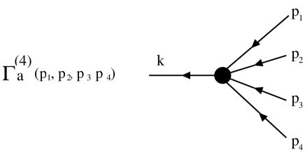
The diagrammatic representation for multi-point propagator and the power spectrum is respectively shown in Figs. 3 and 3.

The construction of the $\Gamma$-expansion is rather transparent, and like Eq. (20), one easily finds the expressions for the higher-order statistical quantities such as bispectrum. Another important point is that one can exploit the asymptotic properties of the propagators $\Gamma^{(p)}$ beyond perturbation theory expansions. To be precise, in the high-$k$ limit, higher-order contributions can be systematically computed at all orders, and as a result of summing up all the contributions, the multi-point propagators are shown to be exponentially suppressed Bernardeau et al. (2008); Bernardeau et al. (2012a),

$$\Gamma^{(p)}_{a}(\mbox{\boldmath$k$}_{1},\cdots,\mbox{\boldmath$k$}_{p};\eta)$$

$$\qquad\stackrel{{\scriptstyle k\to\infty}}{{\longrightarrow}}\exp\left\{-\frac{k^{2}\sigma_{\rm d}^{2}e^{2\eta}}{2}\right\}\Gamma^{(p)}_{a,{\rm tree}}(\mbox{\boldmath$k$}_{1},\cdots,\mbox{\boldmath$k$}_{p};\eta)$$ (22)

with $k=|\mbox{\boldmath$k$}_{1}+\cdots+\mbox{\boldmath$k$}_{p}|$. This is the generalization of the result for the two-point propagator in Ref. Crocce and Scoccimarro (2006b). Here, the quantity $\Gamma^{(p)}_{a,{\rm tree}}$ is the lowest-order non-vanishing propagator obtained from the standard PT calculation, and $\sigma_{\rm d}$ is the one-dimensional root-mean-square of the displacement field defined by,

$$\sigma_{\rm d}^{2}=\frac{1}{3}\int\frac{d^{3}\mbox{\boldmath$q$}}{(2\pi)^{3}}\,\frac{P_{0}(q)}{q^{2}}.$$ (23)

The form of Eq. (22) does not however provide a good description of the propagators at all scale. At low-$k$ the propagators are expected to approach their standard PT expressions that can be written formally,

$$\Gamma_{a}^{(p)}(\mbox{\boldmath$k$}_{1},\cdots,\mbox{\boldmath$k$}_{p};\eta)=\Gamma_{a,{\rm tree}}^{(p)}(\mbox{\boldmath$k$}_{1},\cdots,\mbox{\boldmath$k$}_{p};\eta)$$

$$\qquad\qquad\qquad\qquad+\sum_{n=1}^{\infty}\Gamma_{a,n\mbox{-}{\rm loop}}^{(p)}(\mbox{\boldmath$k$}_{1},\cdots,\mbox{\boldmath$k$}_{p};\eta).$$ (24)

For the dominant growing-mode contribution we are interested in, each correction term is expressed in terms of the standard PT kernels as,

$$\Gamma^{(p)}_{a,{\rm tree}}(\mbox{\boldmath$k$}_{1},\cdots,\mbox{\boldmath$k$}_{p};\eta) =e^{p\,\eta}\,F_{a,{\rm sym}}^{(p)}(\mbox{\boldmath$k$}_{1},c\dots,\mbox{\boldmath$k$}_{p}),$$ (25)

for the tree-level contribution, and

$$\Gamma_{a,n\mbox{-}{\rm loop}}^{(p)}(\mbox{\boldmath$k$}_{1},\cdots,\mbox{\boldmath$k$}_{p};\eta) =e^{(2n+p)\,\eta}\,c_{n}^{(p)}\int\frac{d^{3}\mbox{\boldmath$p$}_{1}\cdots d^{3}\mbox{\boldmath$p$}_{n}}{(2\pi)^{3n}}\,F_{a,{\rm sym}}^{(2n+p)}(\mbox{\boldmath$p$}_{1},-\mbox{\boldmath$p$}_{1},\cdots,\mbox{\boldmath$p$}_{n},-\mbox{\boldmath$p$}_{n},\mbox{\boldmath$k$}_{1},\cdots,\mbox{\boldmath$k$}_{p})P_{0}(p_{1})\cdots P_{0}(p_{n})$$

$$\equiv e^{(2n+p)\,\eta}\,\,\overline{\Gamma}_{a,n\mbox{-}{\rm loop}}^{(p)}(\mbox{\boldmath$k$}_{1},\cdots,\mbox{\boldmath$k$}_{p})$$ (26)

for the $n$-loop order contributions, where the coefficient $c_{n}^{(p)}$ is given by $c_{n}^{(p)}=\,_{(2n+p)}C_{p}\ (2n-1)!!$ where is the binomial coefficient. The graphical representation of the standard PT expansion is shown in Fig. 5. The important remark in Eq. (26) is that each perturbative correction possesses the following asymptotic form,

$$\Gamma^{(p)}_{a,n\mbox{-}{\rm loop}}\stackrel{{\scriptstyle k\to\infty}}{{\longrightarrow}}\frac{1}{n!}\left(-\frac{k^{2}\sigma_{\rm d}^{2}e^{2\eta}}{2}\right)^{n}\Gamma^{(p)}_{a,n\mbox{-}{\rm tree}},$$ (27)

which consistently recovers the expression (22) when we sum up all the loop contributions. This indicates the existence of a matching scheme which smoothly interpolates between the low-$k$ and high-$k$ results for any multi-point propagator. Such a scheme has been proposed in Ref Bernardeau et al. (2012b) where a novel regularized scheme, in which the low- and high-$k$ behaviors are jointly reproduced, is derived. The construction of the regularized propagator is totally unambiguous. They can incorporate an arbitrary number of loop corrections.

Restricting the results to the growing mode contributions, the regularized propagators are expressed in a transparent way in terms of the standard PT results, and one gets

$$\Gamma_{a,{\rm reg}}^{(p)}(\mbox{\boldmath$k$}_{1},\cdots,\mbox{\boldmath$k$}_{p};\eta)=e^{p\,\eta}\left[F^{(p)}_{a,{\rm sym}}(\mbox{\boldmath$k$}_{1},\cdots,\mbox{\boldmath$k$}_{p})\left\{1+\frac{k^{2}\sigma_{\rm d}^{2}e^{2\eta}}{2}\right\}+e^{2\eta}\,\overline{\Gamma}^{(p)}_{a,{\rm 1\mbox{-}loop}}(\mbox{\boldmath$k$}_{1},\cdots,\mbox{\boldmath$k$}_{p})\right]\exp\left\{-\frac{k^{2}\sigma_{\rm d}^{2}e^{2\eta}}{2}\right\},$$ (28)

which consistently reproduces one-loop PT results at low-$k$. An example of the regularized propagator valid at one-loop order is diagrammatically shown in Fig. 5. This construction is easily generalized to include the higher-order PT corrections at low-$k$. For instance, the regularized propagator including the corrections up to the two-loop order becomes,

$$\Gamma_{a,{\rm reg}}^{(p)}(\mbox{\boldmath$k$}_{1},\cdots,\mbox{\boldmath$k$}_{p};\eta)=e^{p,\eta}\left[F^{(p)}_{a,{\rm tree}}(\mbox{\boldmath$k$}_{1},\cdots,\mbox{\boldmath$k$}_{p})\left\{1+\frac{k^{2}\sigma_{\rm d}^{2}e^{2\eta}}{2}+\frac{1}{2}\left(\frac{k^{2}\sigma_{\rm d}^{2}e^{2\eta}}{2}\right)^{2}\right\}\right.$$

$$\left.\qquad\qquad\qquad+\,e^{2\eta}\,\overline{\Gamma}^{(p)}_{\rm 1\mbox{-}loop}(\mbox{\boldmath$k$}_{1},\cdots,\mbox{\boldmath$k$}_{p})\left\{1+\frac{k^{2}\sigma_{\rm d}^{2}e^{2\eta}}{2}\right\}+e^{4\eta}\,\overline{\Gamma}^{(p)}_{\rm 2\mbox{-}loop}(\mbox{\boldmath$k$}_{1},\cdots,\mbox{\boldmath$k$}_{p})\right]\exp\left\{-\frac{k^{2}\sigma_{\rm d}^{2}e^{2\eta}}{2}\right\}.$$ (29)

Note that the functions $\overline{\Gamma}^{(p)}_{n\mbox{-}{\rm loop}}$ are the scale-dependent part of the propagator defined by Eq. (26).

Figure 4: Diagrammatic representation of the standard PT expansion for three-point propagator, $\Gamma_{a}^{(2)}$. For fastest growing-mode contribution, the standard PT kernels, $F_{a,{\rm sym}}^{(n)}$, form the basic pieces of PT expansion, depicted as incoming lines connected to a single outgoing line at the shaded circle. In the case of $\Gamma_{a}^{(2)}$, the leading-order contribution is $F_{a,{\rm sym}}^{(2)}$, and successively the kernels $F_{a,{\rm sym}}^{(4)}$ and $F_{a,{\rm sym}}^{(6)}$ appear as higher-order contributions, for which pairs of the incoming lines are glued at the crossed circle, which indicates the initial power spectrum $P_{0}$, forming closed loops.

Figure 5: Diagrammatic representation of the regularized three-point propagator, $\Gamma_{a,{\rm reg}}^{(2)}$. In the high-$k$ limit, the higher-loop contribution for three-point propagator behaves like Eq. (27), indicating that each loop diagram ($\Gamma^{(2)}_{a,n\mbox{-}{\rm loop}}$) is effectively split into tree diagram ($F_{a,{\rm sym}}^{(2)}$) and self-loop diagram ($\{-(k\sigma_{\rm d})^{2}/2\}^{n}/n!$), the latter of which is depicted as open loops. Systematically summing up all the higher-loop contributions, we recover Eq. (22), which is graphically shown as the infinite sum of open-loop diagrams in the brace. To reproduce the standard PT result at low-$k$, the one-loop diagram is inserted in the bracket, and the tree diagram is multiplied by the counter term $\{1+(k\sigma_{\rm d})^{2}/2\}$.

III Power spectrum calculation from regularized $\Gamma$-expansion

III.1 Power spectrum at two-loop order

Since the proposed regularized propagators preserve the expected low-$k$ and high-$k$ behaviors, the convergence of the $\Gamma$-expansion adopting the regularization scheme would be much better than the standard PT expansion. In this paper, applying this regularized PT treatment, we will explicitly demonstrate the power spectrum calculations at two-loop order, and comparing those predictions with $N$-body simulations, the validity and precision of PT treatment are discussed. From Eq. (20), the explicit expression for the power spectrum valid up to the two-loop order becomes,

$$P_{ab}(k;\eta)=\Gamma_{a,{\rm reg}}^{(1)}(k;\eta)\Gamma_{b,{\rm reg}}^{(1)}(k;\eta)P_{0}(k)+2\int\frac{d^{3}\mbox{\boldmath$q$}}{(2\pi)^{3}}\,\Gamma_{a,{\rm reg}}^{(2)}(\mbox{\boldmath$q$},\mbox{\boldmath$k$}-\mbox{\boldmath$q$};\eta)\Gamma_{b,{\rm reg}}^{(2)}(\mbox{\boldmath$q$},\mbox{\boldmath$k$}-\mbox{\boldmath$q$};\eta)P_{0}(q)P_{0}(|\mbox{\boldmath$k$}-\mbox{\boldmath$q$}|)$$

$$\qquad\qquad\qquad\qquad+6\int\frac{d^{6}\mbox{\boldmath$p$}d^{3}\mbox{\boldmath$q$}}{(2\pi)^{6}}\,\Gamma_{a,{\rm reg}}^{(3)}(\mbox{\boldmath$p$},\mbox{\boldmath$q$},\mbox{\boldmath$k$}-\mbox{\boldmath$p$}-\mbox{\boldmath$q$};\eta)\Gamma_{b,{\rm reg}}^{(3)}(\mbox{\boldmath$p$},\mbox{\boldmath$q$},\mbox{\boldmath$k$}-\mbox{\boldmath$p$}-\mbox{\boldmath$q$};\eta)P_{0}(p)P_{0}(q)P_{0}(|\mbox{\boldmath$k$}-\mbox{\boldmath$p$}-\mbox{\boldmath$q$}|)$$ (30)

with the regularized propagators given by

$$\Gamma_{a,{\rm reg}}^{(1)}(k;\eta)=e^{\eta}\left[1+\frac{k^{2}\sigma_{\rm d}^{2}e^{2\eta}}{2}+\frac{1}{2}\left(\frac{k^{2}\sigma_{\rm d}^{2}e^{2\eta}}{2}\right)^{2}+e^{2\eta}\,\overline{\Gamma}^{(1)}_{a,{\rm 1\mbox{-}loop}}(k)\left\{1+\frac{k^{2}\sigma_{\rm d}^{2}e^{2\eta}}{2}\right\}+e^{4\eta}\,\overline{\Gamma}^{(1)}_{a,{\rm 2\mbox{-}loop}}(k)\right]\exp\left\{-\frac{k^{2}\sigma_{\rm d}^{2}e^{2\eta}}{2}\right\},$$ (31)

$$\Gamma_{a,{\rm reg}}^{(2)}(\mbox{\boldmath$q$},\mbox{\boldmath$k$}-\mbox{\boldmath$q$};\eta)=e^{2\eta}\left[F_{a,{\rm sym}}^{(2)}(\mbox{\boldmath$q$},\mbox{\boldmath$k$}-\mbox{\boldmath$q$})\left\{1+\frac{k^{2}\sigma_{\rm d}^{2}e^{2\eta}}{2}\right\}+e^{2\eta}\,\overline{\Gamma}^{(2)}_{a,{\rm 1\mbox{-}loop}}(\mbox{\boldmath$q$},\mbox{\boldmath$k$}-\mbox{\boldmath$q$})\right]\exp\left\{-\frac{k^{2}\sigma_{\rm d}^{2}e^{2\eta}}{2}\right\},$$ (32)

$$\Gamma_{a,{\rm reg}}^{(3)}(\mbox{\boldmath$p$},\mbox{\boldmath$q$},\mbox{\boldmath$k$}-\mbox{\boldmath$p$}-\mbox{\boldmath$q$};\eta)=e^{3\eta}\,F_{a,{\rm sym}}^{(3)}(\mbox{\boldmath$p$},\mbox{\boldmath$q$},\mbox{\boldmath$k$}-\mbox{\boldmath$p$}-\mbox{\boldmath$q$})\exp\left\{-\frac{k^{2}\sigma_{\rm d}^{2}e^{2\eta}}{2}\right\}.$$ (33)

Note that the higher-order contributions up to the two- and one-loop order of the propagators are respectively included in the expression of the regularized propagators $\Gamma_{a,{\rm reg}}^{(1)}$ and $\Gamma_{a,{\rm reg}}^{(2)}$, consistently with the $\Gamma$-expansion at two-loop order.

The power spectrum expression involves many integrals, but, most of them are reduced to two- or three-dimensional integrals if one uses the analytic expressions for the kernels of higher-loop corrections $\overline{\Gamma}$ in the regularized propagator. We use the expression in Ref. Bernardeau et al. (2012) to evaluate $\overline{\Gamma}^{(2)}_{\rm 1\mbox{-}loop}$, and adopt the fitting functions for the kernel of $\overline{\Gamma}^{(1)}_{\rm 2\mbox{-}loop}$ (see Bernardeau et al. (2012)). We then apply the method of Gaussian quadrature to the numerical evaluation of the low-dimensional integrals. A bit cumbersome is the integral containing $\Gamma^{(3)}$. While it can be reduced to a four-dimensional integral in principle, the expression of the resulting kernel would be very cumbersome and might not be suited for practical calculation. We thus adopt the Monte Carlo technique of quasi-random sampling using the CUBA library Hahn (2005), and evaluate the five-dimensional integral directly.

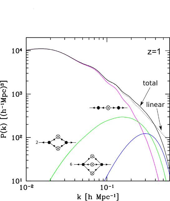
Fig. 6 illustrates an example how each correction term in the regularized $\Gamma$-expansion contributes to the total power spectrum. The plotted result is the density power spectrum, $P_{11}$, and the contribution of the term involving each multi-point propagator is separately shown. The three corrections contribute to the power spectrum at different scales, and the higher-order terms involving $\Gamma^{(2)}_{\rm reg}$ and $\Gamma^{(3)}_{\rm reg}$ are well-localized, each producing one bump. This is a clear manifestation of the result of the regularized PT treatment, and it resembles what the RPT calculations by Ref. Crocce and Scoccimarro (2008) give.

In the next section, the results of the regularized $\Gamma$-expansion will be compared with $N$-body simulations. But, before doing that, we will give several remarks and comments on the computation of the power spectrum in the subsequent subsection.

Figure 6: Contribution of multi-point propagators to the power spectrum, $P(k)=P_{11}(k)$ at $z=1$. Magenta, green, and blue curves represent the power spectrum contributions from the first, second, and third terms at the right-hand-side of Eq. (30), respectively, each of which just corresponds to the diagram in Fig. 3, involving $\Gamma_{\rm reg}^{(1)}$, $\Gamma_{\rm reg}^{(2)}$, and $\Gamma_{\rm reg}^{(3)}$. Summing up these contributions, total power spectrum is shown in black solid line. For reference, linear power spectrum is also plotted as dotted line.

III.2 Effect of running UV cutoff for $\sigma_{\rm d}$

Figure 7: Sensitivity of the power spectrum prediction at $z=1$ to the UV cutoff in the estimation of $\sigma_{\rm d}$. Top panel shows each contribution of the power spectrum corrections involving $\Gamma^{(1)}$ (magenta), $\Gamma^{(2)}$ (green), and $\Gamma^{(3)}$ (blue), respectively. Bottom panel shows the total sum of power spectrum divided by the smooth reference power spectrum, $P_{\rm no\mbox{-}wiggle}(k)$, which is calculated from the no-wiggle formula of the linear transfer function in Ref. Eisenstein and Hu (1998). In each case, top lines represent the results obtained by setting $\sigma_{\rm d}=0$, while undermost lines show the cases adopting the value of $\sigma_{\rm d}$ without UV cutoff. The middle six lines represent the cases adopting the running UV cutoff in estimating $\sigma_{\rm d}$, with cutoff $k_{\Lambda}(k)=k$, $k/2$, $k/3$, $k/5$, $k/10$, and $k/20$ (from bottom to top). As a reference, linear theory prediction is also plotted in both panels (dotted).

Since the shape of the power spectrum given by Eq. (30) significantly depends on the exponential damping in the regularized propagators, we first comment on the effect of this function. As it has been shown, the exponential function arises from the summation of infinite series of perturbations at all order in the high-$k$ limit. Recently, Ref. Bernardeau et al. (2012a) advocated that this exponential function can be interpreted as the result of resummation at hard part (high-$k$), and the displacement dispersion $\sigma_{\rm d}$ in the exponent must be evaluated in a consistent way that the domain of the integral is restricted to a soft part (low-$k$). This implies that depending on the scale of our interest, the boundary of the soft and hard domains can be changed, and the resulting quantity $\sigma_{\rm d}$ should be regarded as a scale-dependent function.

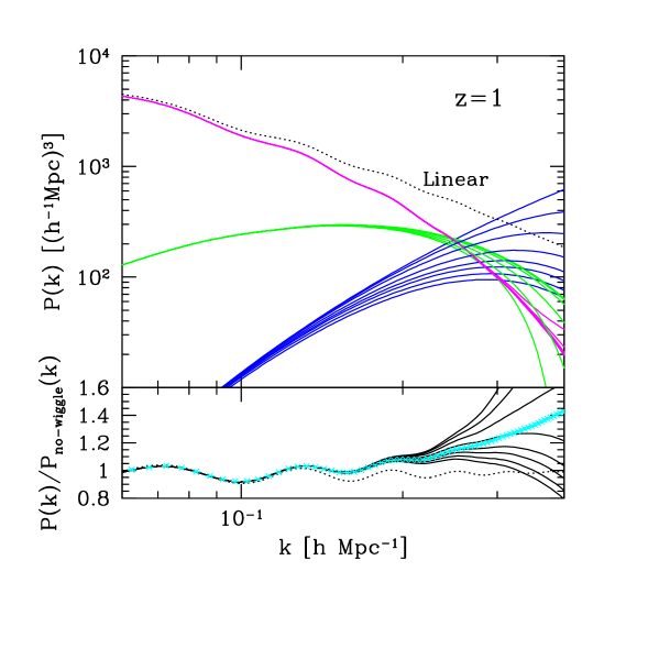
In Fig. 7, we examine the impact of the scale-dependent $\sigma_{\rm d}$ on the power spectrum at $z=1$. Plotted results are the contributions of the power spectrum corrections (upper) and the total power spectrum divided by the smooth reference linear spectrum (bottom). Here, we evaluate $\sigma_{\rm d}$ by introducing the running UV cutoff $k_{\Lambda}(k)$:

$$\sigma_{\rm d}^{2}(k)=\int_{0}^{k_{\Lambda}(k)}\frac{dq}{6\pi^{2}}\,P_{0}(q).$$ (34)

Various curves in Fig. 7 represent the results with different prescription for the running UV cutoff. The correction involving the four-point propagator $\Gamma_{\rm reg}^{(3)}$ is most sensitively affected by the running cutoff, and the resulting power spectrum significantly varies at scales $k\gtrsim 0.2\,h$Mpc^-1. This is because the exponential damping manifests itself at the scale $k\sim 1/(e^{\eta}\sigma_{\rm d})$ where the contribution from $\Gamma_{\rm reg}^{(3)}$, which contains no relevant terms counteracted with the exponential damping, becomes significant among the three corrections.

In the bottom panel of Fig. 7, we also plot the result of $N$-body simulations (see Sec. IV.1). The comparison with simulation suggests that the PT calculation with running cutoff $k_{\Lambda}\sim k/2-k/5$ is favored, although there is no clear physical reason why this is so. Strictly speaking, the running IR cutoff might also be introduced in evaluating all the integrals in the power spectrum expression, so as to consistently discriminate between the contributions coming from soft and hard parts. Moreover, the running cutoff $k_{\Lambda}$ may also depend on the redshift. These complications mostly come from the ambiguity of the boundary between soft and hard domains in our regularization scheme. For practical purpose to the cosmological application, we postpone these issues to future investigation, and take a rather phenomenological approach. Hereafter, the running cutoff is only introduced in evaluating $\sigma_{\rm d}$, and we evaluate it according to Eq. (34), setting the cutoff scale to $k_{\Lambda}=k/2$. With this treatment, we will see later that the PT prediction becomes improved compared to the standard PT calculation, and it reproduces the $N$-body results quite well at any redshift.

Figure 8: Sensitivity of the power spectrum prediction to the UV (left) and IR (right) cutoff. In each panel, the ratio of power spectrum, $P(k)/P_{\rm no\mbox{-}wiggle}(k)$, is plotted as function of $k$ at $z=1$ (left) and $0.35$ (right). In evaluating the integrals of the power spectrum corrections, the maximum wavenumber for the range of the integral is set to $2\pi$ (green), $\pi$ (cyan), and $\pi/2$ (blue) $h$ Mpc^-1 in the left panel, while in the right panel, we change the minimum wavenumber $k_{\rm min}$ to $k_{\rm min}=2\pi/L_{\rm box}$ with $L_{\rm box}=2,048$ (green), $1,024$ (cyan), and $512\,h^{-1}$ Mpc (blue). The magenta lines indicate the results adopting the default set of parameters $(k_{\rm min},k_{\rm max})=(5\times 10^{-4},10)\,h$ Mpc^-1.

III.3 Sensitivity to IR and UV cutoff

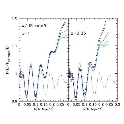
In computing the power spectrum, except for $\sigma_{\rm d}$, the domain of each integral in Eq. (30) are usually taken broad enough so as to ensure the convergence of the results. In comparison with $N$-body simulations, however, a care must be taken because the available Fourier modes in simulations are restricted depending on the simulation box size and/or mesh size of Fourier transform, which affect both the efficiency of mode transfer and strength of mode coupling. The evolved result of the power spectrum would thus be changed, and it should be carefully compared with PT calculation, taking the finite resolution into consideration. Here, focusing on the BAO scales, we briefly discuss the sensitivity of the PT calculation to the IR and UV cutoff in the integrals.

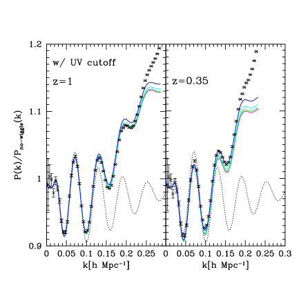
Fig. 8 shows the variation of the power spectra with respect to the UV (left) and IR (right) cutoff. In general, the kernel of integrals becomes broader for higher-loop corrections, and thus the two-point propagator $\Gamma^{(1)}_{\rm reg}$ containing the two-loop contribution is sensibly affected by the UV cutoff. Note that the signs of one- and two-loop corrections in $\Gamma^{(1)}_{\rm reg}$ are opposite at BAO scales. Hence, as decreasing the cutoff wavenumber $k_{\rm max}$, the cancellation of each contribution is relatively relaxed, and the power spectrum amplitude gets increased. On the other hand, due to the lack of the long-wave modes, the IR cutoff not only decreases each contribution of the loop integrals, but also reduces $\sigma_{\rm d}$, leading to a slight suppression of the exponential damping. The net effect of the IR cutoff, especially at small scales $k\gtrsim 0.2\,h\,$Mpc^-1, is that the latter overcomes the former, and the total power spectrum is slightly enhanced.

These results imply that the effect of UV and IR cutoff not only affects the power spectrum shape at small scales, but also causes a slight offset in power spectrum amplitude at moderately large scales, $k\sim 0.1\,h$Mpc^-1. The size of these effects is basically small, but would not be negligible in a percent-level comparison. Based on this remark, in what follows, we adopt the cutoff scales $(k_{\rm min},k_{\rm max})=(5\times 10^{-4},10)\,h$ Mpc^-1 as default parameters to compute the power spectra. With this setup, RegPT calculation gives a mostly convergent result, which can be compared with high-resolution $N$-body simulations with a large box size.

III.4 Comparison with MPTbreeze

In Ref. Crocce et al. (2012), mptbreeze, an alternative scheme has been proposed for the construction of power spectra that is based on the same multi-point propagator expansion. This proposition is, however, based on simplified assumptions regarding the behavior of the multi-point propagators. More specifically, in mptbreeze, the propagators are assumed to take the form,

$$\Gamma_{a,{\rm reg}}^{(p)}(\mbox{\boldmath$q$}_{1},\dots,\mbox{\boldmath$q$}_{p-1},\mbox{\boldmath$k$}-\mbox{\boldmath$q$}_{1\cdots(p-1)};\eta)=e^{p\,\eta}\,F_{a,{\rm sym}}^{(p)}(\mbox{\boldmath$q$}_{1},\dots,\mbox{\boldmath$q$}_{p-1},\mbox{\boldmath$k$}-\mbox{\boldmath$q$}_{1\cdots(p-1)})\,\exp\left\{f_{a}(k)e^{2\eta}\right\},$$ (35)

where $f_{1}(k)$ and $f_{2}(k)$ are the one-loop corrections to the density and velocity propagators, respectively. This form corresponds to the late-time original expression of the exponentiation scheme initially put forward in Ref. Crocce and Scoccimarro (2006b). It is shown in Refs. Bernardeau et al. (2012b); Bernardeau et al. (2012) that at one-loop order, this prescription gives nearly identical result for the two-point propagator to the prescription proposed in Ref. Crocce and Scoccimarro (2006b). The mptbreeze prescription, however, ignores the impact of two-loop PT corrections on the two-point propagators. From the results presented in Bernardeau et al. (2012), it implies that mptbreeze might be outperformed by RegPT at $z\gtrsim 1$. On the other hand, the predictions of that scheme are made more robust because they are less sensitive to the UV part of the linear spectrum as discussed in that paper. Furthermore, the one-loop correction for the three- and four-point propagators are treated in an effective way. These simplified assumptions allow a more rapid calculations of the set of diagrams. It takes just a few seconds to get the expected shape in this scheme. The computational time is, however, rather comparable to the fast implementation of RegPT  which we will present in Sec. V.

IV Comparison with $N$-body simulations

We are now in position to present quantitative comparisons between RegPT calculations and $N$-body simulations. After briefly describing the $N$-body simulations in Sec. IV.1, we show the results of power spectrum and two-point correlation function in Sec. IV.2 and IV.3, respectively. Precision and validity of the PT predictions are discussed in detail.

Figure 9: Comparison of power spectrum results between $N$-body simulations and RegPT calculations. In each panel, the results at $z=3$, $2$, $1$, and $0.35$ are shown (from top to bottom). Left panel shows the ratio of power spectrum to the smooth linear spectrum, $P(k)/P_{\rm no\mbox{-}wiggle}(k)$, where the reference spectrum $P_{\rm no\mbox{-}wiggle}(k)$ is calculated from the no-wiggle formula of the linear transfer function in Ref. Eisenstein and Hu (1998). Solid lines are the RegPT results, while dotted lines represent the linear theory predictions. Right panel plots the difference between $N$-body and RegPT results normalized by the no-wiggle spectrum, i.e., $[P_{\rm N\mbox{-}body}(k)-P_{\rm RegPT}(k)]/P_{\rm no\mbox{-}wiggle}(k)$. In each panel, The vertical arrows respectively indicate the maximum wavenumber below which a percent-level agreement with $N$-body simulation is achieved with Lagrangian resummation theory Matsubara (2008a); Okamura et al. (2011) and closure theory Taruya et al. (2009); Taruya and Hiramatsu (2008), including the PT correction up to two-loop order.

Figure 10: Comparison of two-point correlation function between $N$-body and RegPT results at $z=3$, $2$, $1$, and $0.35$ (from bottom to top). In each panel, magenta solid, and black dotted lines represent the prediction from RegPT and linear theory calculations, respectively. Left panel focuses on the behavior around baryon acoustic peak in linear scales, while right panel shows the overall behavior in a wide range of separation in logarithmic scales. Note that in right panel, the resulting correlation function is multiplied by the cube of the separation for illustrative purpose.

Table 1: Cosmological parameters for $N$-body simulations ($\Lambda$CDM)

Name	$L_{\rm box}$	# of particles	$z_{\rm ini}$	# of runs	$\Omega_{\rm m}$	$\Omega_{\Lambda}$	$\Omega_{\rm b}/\Omega_{\rm m}$	$w$	$h$	$n_{s}$	$\sigma_{8}$
wmap5	$2,048h^{-1}$Mpc	$1,024^{3}$	$15$	$60$	0.279	0.721	0.165	-1	0.701	0.96	$0.815_{9}$

IV.1 $N$-body simulations

To compare RegPT calculations with $N$-body simulations, we ran a new set of $N$-body simulations, which will be presented in more detail with an extensive convergence study in Nishimichi et al. (2012). This set of simulations can be regarded as an updated version of the one presented in Taruya et al. (2009) with much larger total volume and a more careful setup to achieve a smaller statistical and systematic error. The data were created by a public $N$-body code GADGET2 Springel (2005) with cubic boxes of side length $2,048\,h^{-1}$Mpc, and $1,024^{3}$ particles. The cosmological parameters adopted in these $N$-body simulations are basically the same as in the previous one, and are determined by the five-year WMAP observations Komatsu et al. (2009) (see Table 1). The initial conditions were generated by a parallelized version of the 2LPT code Crocce et al. (2006), developed in Ref. Valageas and Nishimichi (2011). After several tests given in Ref. Valageas and Nishimichi (2011), a lower initial redshift $z_{\rm init}$ turns out to give a more reliable estimate for the power spectrum at BAO scales, and we thus adopt the initial redshift $z_{\rm init}=15$. With this setup, we have created $60$ independent realizations and the data were stored at redshifts $z=3$, $2$, $1$, and $0.35$. The total volume at each output redshift is $515\,h^{-3}$Gpc³, which is statistically sufficient for a detailed comparison with PT calculations.

We measure both the matter power spectrum and the correlation function. For the power spectrum, we adopt the Cloud-in-Cells interpolation, and construct the Fourier transform of the density field assigned on the $1,024^{3}$ grids. As for the estimation of the two-point correlation function, we adopt the grid-based calculation using the Fast Fourier Transformation Taruya et al. (2009). Similarly to the power spectrum analysis, we first compute the square of the density field on each grid point in Fourier space. Then, applying the inverse Fourier transformation, we take the average over separation vectors and realizations, and finally obtain the two-point correlation function. The implementation of this method, together with a convergence test, is presented in more detail in Ref .Taruya et al. (2009).

IV.2 Power spectrum

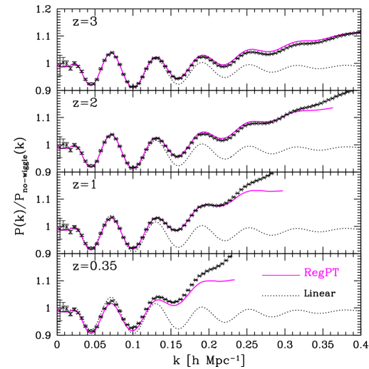
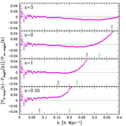
Let us first present the power spectrum results. Left panel of Fig. 9 shows the ratio of the power spectra, $P(k)/P_{\rm no\mbox{-}wiggle}(k)$, while the right panel plots the fractional difference between $N$-body simulations and PT calculations, defined by $[P_{\rm N\mbox{-}body}(k)-P_{\rm PT}(k)]/P_{\rm no\mbox{-}wiggle}(k)$ (where $P_{\rm no\mbox{-}wiggle}(k)$ is calculated from the no-wiggle formula of the linear transfer function in Ref. Eisenstein and Hu (1998)). Overall, the agreement between RegPT and $N$-body simulations is remarkable at low-$k$, and a percent-level agreement is achieved up to a certain wavenumber. For a decreasing redshift, the non-linearities develop and the applicable range of PT calculations inevitably becomes narrower, however, compared to the standard PT predictions, the RegPT result can reproduce the $N$-body trend over an even wider range. Indeed, the range of agreement with $N$-body simulations is rather comparable to other improved PTs including higher-order corrections, such as closure theory Taruya et al. (2009); Taruya and Hiramatsu (2008), and better than some of those predictions. For reference, we compute the power spectra from closure and Lagrangian resummation theory (LRT) Matsubara (2008a); Okamura et al. (2011) at two-loop order, and estimate the range of a percent-level agreement with $N$-body simulations, the results of which are respectively depicted as green and blue vertical arrows in right panel of Fig. 9. Note that at $z=3$, the range of agreement for closure theory exceeds the plotted range, and is not shown here.

Although the RegPT treatment gives a very good performance comparable to or even better than other improved PTs, a closer look at Fig. 9 reveals several sub-percent discrepancies.

• One is the low-$k$ behavior at $z=0.35$, which exhibits a small discrepancy with $N$-body simulation. Our investigations indicate that it is probably due to a poor convergence of standard PT expansion, since the low-$k$ behavior of regularized propagators heavily relies on the standard PT treatment. To be specific, the convergence of $\Gamma^{(1)}_{\rm reg}$ is the main source of this discrepancy. Indeed, if $\Gamma^{(1)}_{\rm reg}$ is computed at one-loop order only, the power spectrum is enhanced, and then N-body results at low-$k$ lie in between the two predictions. The impact of the high order PT corrections to the two-point propagator are specifically studied in a separate publication, Bernardeau et al. (2012).

• Another discrepancy can be found in the high-$z$ results, which temporally overshoot the $N$-body results at mid-$k$ regime ($k\sim 0.2$ – $0.3\,h$ Mpc^-1). It is unlikely to be due to a poor convergence of standard PT expansion. We rather think that the performances of the $N$-body simulations might be responsible for this (small) discrepancy. We have tested several runs with different resolutions, and found that the low-resolution simulation with a small number of particles tends to underestimate the power at high-$z$. Possible reason for this comes from the precision of force calculation around the intervening scales, where the Tree and Particle-Mesh algorithms are switched, and is mainly attributed to the inaccuracy of the Tree algorithm. Though the intervening scale is usually set at a sufficiently small scale, with a low-resolution simulation, it may affect the large-scale dynamics with noticeable effects at higher redshifts. Systematic studies on the convergence and resolution of $N$-body simulations will be reported elsewhere Nishimichi et al. (2012).

IV.3 Correlation function

We next consider the two-point correlation function, which can be computed from the power spectrum as

$$\xi(r)=\int\frac{dk\,k^{2}}{2\pi^{2}}\,P(k)\,\frac{\sin(kr)}{kr}.$$ (36)

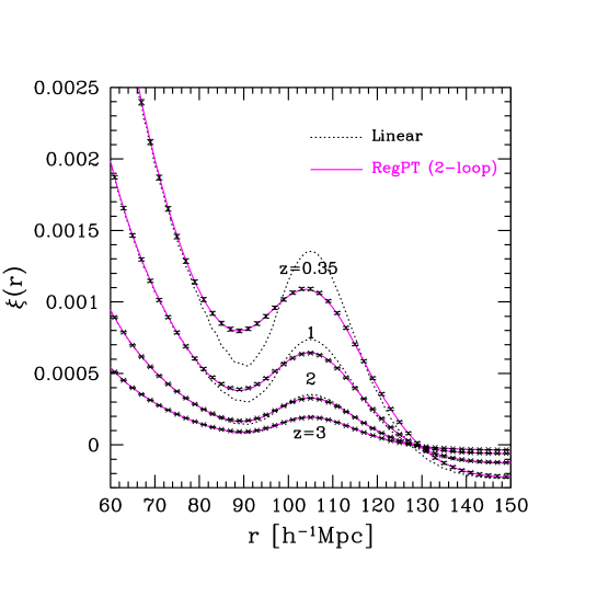
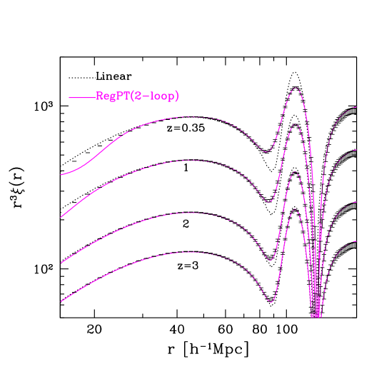
In Fig. 10, left panel focuses on the behaviors around the baryon acoustic peak, while right panel shows the global shape of the two-point correlation function plotted in logarithmic scales, for which $\xi(r)$ has been multiplied by the cube of the separation. The RegPT results agree with $N$-body simulations almost perfectly over the plotted scales. As it is known, the impact of non-linear clustering on the baryon acoustic peak is significant: the peak position becomes slightly shifted to a smaller scale, and the structure of the peak tends to be smeared as the redshift decreases (e.g., Eisenstein et al. (2007); Crocce and Scoccimarro (2008); Smith et al. (2008); Matsubara (2008a)). The RegPT calculation can describe not only the behavior around the baryon acoustic peak but also the small-scale behavior of the correlation function. Note that similar results are also obtained from other improved PT treatments such as closure and LRT. Although the RegPT predictions eventually deviate from simulations at small scales – the result at $z=0.35$ indeed manifests the discrepancy below $r\sim 30\,h^{-1}$ Mpc – the actual range of agreement between RegPT and $N$-body results is even wider than what is naively expected from the power spectrum results. In fact, it has been recently advocated by several authors that with several improved PT treatments, the one-loop calculation is sufficient to accurately describe the two-point correlation function (e.g., Okamura et al. (2011); Taruya et al. (2009); Reid and White (2009)). We have checked that the RegPT treatment at one-loop order can give a satisfactory result close to the two-loop result, and the prediction including the two-loop corrections only slightly improves the agreement with $N$-body simulations at small scales. This is good news for practical purposes in the sense that we do not necessarily have to evaluate the multi-dimensional integrals for the accurate prediction of two-point correlation function in the weakly non-linear regime. Nevertheless, in this work, we keep the two-loop contributions in the computed contributions. The computational costs of the two-loop order will be addressed in the following with the development of a method for accelerated PT calculation at two-loop order.

V RegPT-fast: Accelerated power spectrum calculation

In this section, we present a method that allows accelerated calculations of the required diagrams of the two-loop order RegPT prescription. In principle, the power spectra calculations in the context of RegPT require multi-dimensional integrations that cannot be done before-hand as they fully depend on the linear power spectra. It is however possible to obtain the required quantities much more rapidly provided we know the answer for a close enough model.

The key point in this approach is to utilize the fact that the nonlinear RegPT power spectrum is a well-defined functional form of the linear power spectrum. Each of the diagram that has to be computed is of quadratic, cubic, etc. order with respect to the linear power spectrum with a kernel that, although complicated, can be explicitly given. It is then easy to Taylor expand each of these terms with respect to the linear power spectrum. In principle one then just needs to prepare, in advance, a set of the RegPT results for some fiducial cosmological models, and then take the difference between fiducial and target initial power spectra for which we want to calculate the non-linear power spectrum. These differences involve only one-dimensional integrals at the first order in the Taylor expansion.

In the following, we present the detail of the implementation of this approach illustrating it with the one-loop calculation case.

V.1 Power spectrum reconstruction from fiducial model

While our final goal is to present the fast PT calculation at two-loop order, in order to get insights into the implementation of this calculation, we consider the power spectrum at one-loop order. The complete expressions needed for the fast PT calculation at two-loop order, together with the prescription how to implement it, is presented in Appendix A.

Compared to the expressions given in Eq. (30), the power spectrum at one-loop order of the $\Gamma$-expansion reduces to

$$P_{ab}(k;\eta)=\Gamma_{a,{\rm reg}}^{(1)}(k;\eta)\Gamma_{b,{\rm reg}}^{(1)}(k;\eta)P_{0}(k)+2\int\frac{d^{3}\mbox{\boldmath$q$}}{(2\pi)^{3}}\,\Gamma_{a,{\rm reg}}^{(2)}(\mbox{\boldmath$q$},\mbox{\boldmath$k$}-\mbox{\boldmath$q$};\eta)\Gamma_{b,{\rm reg}}^{(2)}(\mbox{\boldmath$q$},\mbox{\boldmath$k$}-\mbox{\boldmath$q$};\eta)P_{0}(q)P_{0}(|\mbox{\boldmath$k$}-\mbox{\boldmath$q$}|)$$ (37)

with the regularized propagators $\Gamma^{(1)}_{\rm reg}$ and $\Gamma^{(2)}_{\rm reg}$ valid at one-loop order being:

$$\Gamma_{a,{\rm reg}}^{(1)}(k;\eta)=e^{\eta}\left[1+\frac{k^{2}\sigma_{\rm d}^{2}e^{2\eta}}{2}+e^{2\eta}\,\overline{\Gamma}^{(1)}_{a,{\rm 1\mbox{-}loop}}(k)\right]$$

$$\qquad\qquad\qquad\qquad\qquad\qquad\times\exp\left\{-\frac{k^{2}\sigma_{\rm d}^{2}e^{2\eta}}{2}\right\},$$ (38)

$$\Gamma_{a,{\rm reg}}^{(2)}(\mbox{\boldmath$q$},\mbox{\boldmath$k$}-\mbox{\boldmath$q$};\eta)=e^{2\eta}F_{a,{\rm sym}}^{(2)}(\mbox{\boldmath$q$},\mbox{\boldmath$k$}-\mbox{\boldmath$q$})\,$$

$$\qquad\qquad\qquad\qquad\qquad\qquad\times\exp\left\{-\frac{k^{2}\sigma_{\rm d}^{2}e^{2\eta}}{2}\right\}.$$ (39)

Note that the quantity $\overline{\Gamma}^{(1)}_{a,{\rm 1\mbox{-}loop}}$ is defined in Eq. (26), and explicitly given by

$$\overline{\Gamma}^{(1)}_{a,{\rm 1\mbox{-}loop}}(k)=3\int\frac{d^{3}\mbox{\boldmath$q$}}{(2\pi)^{3}}\,F_{a,{\rm sym}}^{(3)}(\mbox{\boldmath$q$},-\mbox{\boldmath$q$},\mbox{\boldmath$k$})P_{0}(q).$$ (40)

Thus, in Eq. (37), there apparently appear two contributions which involve multi-dimensional integrals; $\overline{\Gamma}^{(1)}_{a,{\rm 1\mbox{-}loop}}$ in the regularized propagator $\Gamma_{a,{\rm reg}}^{(1)}$, and the second term at the right-hand side. Although these contributions are known to be further reduced to one-, and two-dimensional integrals (e.g., Refs Bernardeau et al. (2012b); Crocce and Scoccimarro (2006b); Taruya and Hiramatsu (2008)), respectively, for the sake of this presentation we keep the expressions as in their original form.

As it has been mentioned earlier, the key idea of accelerated calculation is to prepare a set of RegPT results for fiducial cosmological models. Let us denote the initial power spectrum for fiducial cosmology by $P_{0,{\rm fid}}(k)$. And we denote the initial spectrum for the target cosmological model, for which we want to calculate the non-linear power spectrum, by $P_{0,{\rm target}}(k)$. For the moment, we assume that the difference between those spectra is small enough. Then, we may write

$$P_{0,{\rm target}}(k)=P_{0,{\rm fid}}(k)+\delta P_{0}(k).$$ (41)

Hereafter, we focus on the power spectrum of density field, $P_{11}$, and drop the subscript. Substituting the above expression into Eqs. (37)-(39), the non-linear power spectrum for the target model is symbolically written as

$$P_{\rm target}(k;\eta)=P_{\rm un\mbox{-}pert}[k,\eta,\sigma_{\rm d,target};P_{0,{\rm fid}}(k)]$$

$$\qquad\qquad\qquad\qquad+P_{\rm corr}[k,\eta,\sigma_{\rm d,target};\delta P_{0}(k)].$$ (42)

Here, the first term at the right hand side is the un-perturbed part of the one-loop power spectrum, which is nothing but the expression (37) adopting the initial power spectrum for fiducial model, $P_{0,{\rm fid}}(k)$, but with the cosmological dependence of the time variable, given by $\eta=\ln D(z)$, being calculated from the target model. Also, the dispersion of displacement field, $\sigma_{\rm d}$, should be replaced with the one for the target model, i.e., $\sigma_{\rm d,target}=[\int dqP_{0,{\rm target}}(q)/(6\pi^{2})]^{1/2}$. In each term of Eq. (37), the scale and time dependence can be separately treated, and thus the un-perturbed power spectrum, $P_{\rm un\mbox{-}perturbed}$, is evaluated algebraically by summing up each contribution, for which we use the precomputed data set in evaluating the scale-dependent function.

In Eq. (42), the contribution $P_{\rm corr}$ includes the non-linear corrections originating from the differences of initial power spectra between fiducial and target cosmological models. To first order in $\delta P_{0}$, we have

$$P_{\rm corr}[k,\eta,\sigma_{\rm d,target};\delta P_{0}(k)]=2\Gamma_{\rm reg}^{(1)}(k;\eta)\,\delta\Gamma_{\rm reg}^{(1)}(k;\eta)\,P_{0,{\rm fid}}(k)+\left[\Gamma_{\rm reg}^{(1)}(k;\eta)\right]^{2}\,\delta P_{0}(k)$$

$$\qquad\qquad\qquad\qquad\qquad\qquad\qquad\qquad+4\int\frac{d^{3}\mbox{\boldmath$q$}}{(2\pi)^{3}}\,\left[\Gamma_{\rm reg}^{(2)}(\mbox{\boldmath$q$},\mbox{\boldmath$k$}-\mbox{\boldmath$q$};\eta)\right]^{2}P_{0,{\rm fid}}(|\mbox{\boldmath$k$}-\mbox{\boldmath$q$}|)\delta P_{0}(q)$$ (43)

In the above expression, The quantity $\sigma_{\rm d}$ appearing in the propagators $\Gamma_{\rm reg}^{(1)}$ and $\Gamma_{\rm reg}^{(2)}$ should be evaluated with the linear power spectrum for the target cosmological model. The perturbed propagator $\delta\Gamma_{\rm reg}^{(1)}$ is expressed as

$$\delta\Gamma_{\rm reg}^{(1)}(k;\eta)=e^{3\eta}\,\delta\overline{\Gamma}^{(1)}(k)\,e^{-k^{2}\sigma_{\rm d,target}^{2}e^{2\eta}/2}$$ (44)

where the kernel of integral in $\delta\overline{\Gamma}^{(1)}$ is the same one as in Eq. (40), but we may rewrite it with

$$\delta\,\overline{\Gamma}^{(1)}(k)=\int\frac{dq\,q^{2}}{2\pi^{2}}\,L_{1}^{(1)}(q,k)\,\delta P_{0}(q)$$ (45)

with the kernel $L_{1}^{(1)}$ given by

$$L_{1}^{(1)}(q,k)=3\,\int\frac{d^{2}\mbox{\boldmath$\Omega$}_{q}}{4\pi}\,F_{1,{\rm sym}}^{(3)}(\mbox{\boldmath$q$},-\mbox{\boldmath$q$},\mbox{\boldmath$k$}).$$ (46)

Since the kernel $L_{1}^{(1)}$ only includes the PT kernel whose cosmological dependence is extremely weak, we can separately prepare the numerical data set for $L_{1}^{(1)}$ in advance . Then, we can use it to compute $\delta\overline{\Gamma}^{(1)}$ for arbitrary $\delta P_{0}$, where the remaining integral to be evaluated is reduced to a one-dimensional integral.

Furthermore, the integral in the last term of Eq. (43) is rewritten with

$$\int\frac{d^{3}\mbox{\boldmath$q$}}{(2\pi)^{3}}\left[\Gamma_{\rm reg}^{(2)}(\mbox{\boldmath$q$},\mbox{\boldmath$k$}-\mbox{\boldmath$q$};\eta)\right]^{2}P_{0,{\rm fid}}(|\mbox{\boldmath$k$}-\mbox{\boldmath$q$}|)\,\delta P_{0}(q)$$

$$\quad=e^{-k^{2}\sigma_{\rm d,target}^{2}e^{2\eta}}\,e^{4\eta}\,\int\frac{dq\,q^{2}}{2\pi^{2}}X^{(2)}(q,k)\,\delta P_{0}(q)$$ (47)

with the function $X^{(2)}$ being

$$X^{(2)}(q,k)=\frac{1}{2}\int_{-1}^{1}d\mu\,\left[F^{(2)}_{\rm sym}(\mbox{\boldmath$q$},\mbox{\boldmath$k$}-\mbox{\boldmath$q$})\right]^{2}\,$$

$$\quad\qquad\qquad\qquad\times P_{0,{\rm fid}}(\sqrt{k^{2}-2kq\mu+q^{2}}),$$ (48)

where the variable $\mu$ is the directional cosine defined by $\mu=(\mbox{\boldmath$k$}\cdot\mbox{\boldmath$q$})/(kq)$. In deriving the above expression, we used the symmetric property of $\Gamma^{(2)}_{\rm reg}$, i.e., $\Gamma^{(2)}_{\rm reg}(\mbox{\boldmath$k$}_{1},\mbox{\boldmath$k$}_{2})=\Gamma^{(2)}_{\rm reg}(\mbox{\boldmath$k$}_{2},\mbox{\boldmath$k$}_{1})$. Since the quantity $X^{(2)}(q,k)$ can be computed in advance, all the integrals involving the power spectrum $\delta P_{0}$ are shown to be effectively reduced to one-dimensional integrals. In other words the only remaining task is to evaluate one-dimensional integrals, which can be done very efficiently.

The practical implementation of this method makes use of another important property of the kernel functions. They indeed have a very simple dependence on a global rescaling of the power spectrum, $P_{0,{\rm fid}}\,\to\,c\,\,P_{0,{\rm fid}}$. It is then possible, without extra numerical computation, to choose the fiducial model among a continuous set of models. The model we choose, that is the normalization factor $c$ we take, is such that the difference $\delta P_{0}(k)$ is as small as possible in the wave-modes of interest. As we will see in Sec. VI it makes the use of this method very efficient.

Note that although the treatment depicted here does not give much impact on the computational cost of the one-loop calculation, we will explicitly show in Appendix A that at two-loop order the PT corrections involving multi-dimensional integrals can be similarly reduced to one-dimensional integrals. In the following, we denote RegPT-fast the implementation of this approach at two-loop order.

Figure 11: Example of the performances of the RegPT-fast approach compared to direct RegPT calculation. Left panel shows the power spectrum divided by the smooth reference spectrum, $P(k)/P_{\rm no\mbox{-}wiggle}(k)$, while right panel plots the correlation function multiplied by the cube of separation, i.e., $r^{3}\,\xi(r)$. In both panels, the results at $z=1$ are shown, together with $N$-body simulations. The RegPT-fast results, computed with prepared data set for fiducial cosmological model, are plotted as magenta solid lines, which almost coincide with those obtained from the rigorous RegPT calculation (magenta solid). As shown in Eq. 42, the RegPT-fast results are divided into two contributions; un-perturbed part ($P_{\rm un\mbox{-}pert}$ or $\xi_{\rm un\mbox{-}pert}$) adopting the wmap3 model as fiducial cosmology, and the correction part ($P_{\rm corr}$ or $\xi_{\rm corr}$) evaluated with the power spectrum difference $\delta P_{0}$. These are respectively plotted as green dashed and cyan dashed lines. For reference, we also show the linearly evolved result of power spectrum difference $\delta P_{0}$ (cyan dashed) and the sum of the contributions $P_{\rm un\mbox{-}pert}+\delta P_{0}$ (cyan solid) in left panel, and their Fourier counterparts in right panel.

V.2 Performances

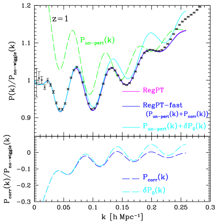
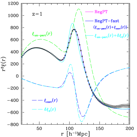
Let us now illustrate the efficiency of the RegPT-fast expansion. Based on the expressions given in Appendix A, we calculate the power spectrum and correlation function at two-loop order. We adopt the best-fit parameters determined by the third-year WMAP result Spergel et al. (2007) as the fiducial cosmological model from which we try to reproduce the RegPT results for the five-year WMAP cosmological model. Cosmological parameters for the fiducial model is listed in Table 2. Compared to the target model in Table 1, the mass density parameter shows a $20\%$ difference, and with $7\%$ enhancement in the power spectrum normalization ($\sigma_{8}$), this leads to a $20$-$30$% difference in the initial power spectrum.

Fig. 11 plots the results of the RegPT-fast calculation (blue) compared to the target RegPT calculation (magenta). We plot, for a specific redshift $z=1$, the ratio of the power spectrum to the smooth reference spectrum, $P(k)/P_{\rm no\mbox{-}wiggle}(k)$, and correlation function multiplied by the cube of separation, $r^{3}\xi(r)$, in left and right panels, respectively. The RegPT-fast results perfectly coincide with RegPT direct calculation, even outside the range of agreement with $N$-body simulations.

Note that the perfect match between RegPT and RegPT-fast results is due to a large extent to the contributions of the higher-order PT in the correction, $P_{\rm corr}$ or $\xi_{\rm corr}$. This appears clearly in the plots of the linear theory correction, $\delta P_{0}=P_{0,{\rm target}}-P_{0,{\rm fid}}$ and its Fourier counterpart $\delta\xi_{0}$ (cyan long-dashed). As shown in cyan solid lines, the total contribution, i.e., the combination of the un-perturbed part plus linear theory correction, somehow resembles the result with direct RegPT calculation, but exhibits a rather prominent oscillatory feature with slightly different phase in power spectrum, leading to a non-negligible discrepancy. Accordingly, in correlation function, the acoustic peak becomes enhanced, and the position of peak is shifted to a small separation. Note finally, that these results could only be achieved with the help of the rescaling properties of the kernel functions. In this particular case the fiducial model has been rescaled as $P_{0,{\rm fid}}\to 1.082\,P_{0,{\rm fid}}$. Rescaling is a key feature of the RegPT-fast method. It will be further discussed in the next section.

Table 2: Cosmological parameters for fiducial models used for the RegPT-fast calculation (see Sec. VI.1).

Name	$\Omega_{\rm m}$	$\Omega_{\Lambda}$	$\Omega_{\rm b}/\Omega_{\rm m}$	$w$	$h$	$n_{s}$	$\sigma_{8}$
wmap3	0.234	0.766	0.175	-1	0.734	0.961	0.760
M001	$0.430_{7}$	$0.569_{2}$	0.150	-0.816	$0.597_{7}$	$0.946_{8}$	$0.816_{1}$
M023	$0.160_{2}$	$0.839_{8}$	$0.181_{7}$	-1.261	$0.869_{4}$	$0.901_{6}$	$0.666_{4}$

Figure 12: Linear power spectra $P_{0}(k)$ for 38 cosmological models Lawrence et al. (2010). Blue, green, and magenta lines are respectively the power spectra of fiducial models wmap3, M001, and M023 used for the RegPT-fastcalculation (see Table 2 for their cosmological parameters).

VI Testing RegPT treatment for varying cosmological models

The purpose of this section is twofold. Our first goal is to explore the validity and applicability of the RegPT-fast scheme. Having shown that the RegPT-fast approach can be used in one specific example, we now want to discuss the usefulness of this treatment from a more practical point of view. To be precise, we want to know how well the RegPT-fast treatment can reproduce rigorous RegPT calculation in a variety of cosmological models.

Our second and natural goal is to test the RegPT scheme itself, whether from direct or fast calculations, against N-body based predictions such that the cosmic emulator.

To do that, we have selected the $38$ cosmological models investigated in Ref. Lawrence et al. (2010) for which we can use the publicly released code, cosmic emulator, that provides interpolated power spectra derived from $N$-body simulations. Let us remind that the cosmological models considered there are sampled from a wide parameter space for flat $w$-CDM cosmology, and lie within the range,

$$0.120<\Omega_{\rm m}h^{2}<0.155,$$

$$0.0215<\Omega_{\rm b}h^{2}<0.0235,$$

$$0.85<n_{\rm s}<1.05,$$

$$-1.30<w<-0.70,$$

$$0.616<\sigma_{8}<0.9.$$

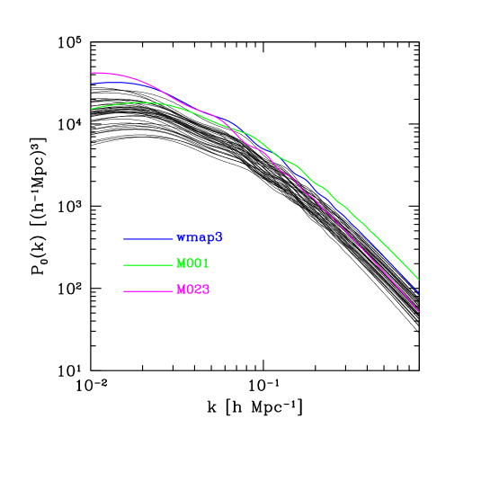
The concrete values of the cosmological parameters in each model are not shown here. Readers can find them in Table 1 of Ref. Lawrence et al. (2010). Fig. 12 shows the linear power spectra $P_{0}(k)$ for the $38$ cosmological models, which have been all produced with CMB Boltzmann code, camb Lewis et al. (2000).

VI.1 Convergence of RegPT-fast

Figure 13: Convergence between the RegPT-fast treatment and the direct RegPT calculations for $38$ cosmological models. The fractional difference of the power spectra between RegPT-fast and RegPT direct calculations, $P_{\rm RegPTfast}(k)/P_{\rm RegPT}(k)-1$, is plotted at $z=1$. Left and right panels respectively show the results adopting the one and three fiducial models.

Figure 14: Ratio of power spectra, $P(k)/P_{\rm no\mbox{-}wiggle}(k)$, at $z=1$ for the cosmological models M000–M017. Solid and dotted lines are obtained from the RegPT-fast and cosmic emulator codes, respectively. The fiducial model used for the RegPT-fast calculation is indicated in each panel. The vertical arrows mean the critical wavenumber $k_{\rm crit}$ defined by Eq. (49), which roughly gives an applicable range of RegPT prediction (see text).

Figure 15: Same as Fig. 14, but for the models M019–M037.

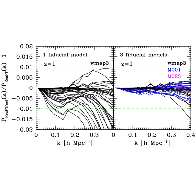
Let us first examine the convergence of the power spectrum calculations between RegPT and RegPT-fast treatments. We ran both the RegPT-fast and RegPT codes, and evaluate the fractional difference between these power spectra, defined by $P_{\rm RegPTfast}(k)/P_{\rm RegPT}(k)-1$. Collecting the results at $z=1$ in each cosmological model, the convergence of the power spectrum calculations for $38$ models is summarized in Fig. 13. In left panel we show the result when only one fiducial model, wmap3, is used. In that case RegPT-fast results tend to underestimate the results from rigorous RegPT calculations at increasing $k$, and most of them eventually exceed the $1\%$ difference, indicated by the green dashed line. This is because the shape of the initial power spectrum in each target model is rather different from that in the fiducial model, and even adjusting the re-scaling parameter $c$ cannot compensate a large power spectrum difference. To be more precise, in most of the models, the shape parameter, defined by $\Gamma=\Omega_{\rm m}h$, is typically larger than the one in the fiducial model. As a consequence, even if we adjust the power spectrum at large scales to match the one in the target model, the difference $|\delta P_{0}|$ can become large as increasing $k$, leading to a failure of the perturbative reconstruction by RegPT-fast.

To remedy this situation, a simple but efficient approach is to enlarge our set of fiducial models with $\Gamma$-parameters that differ from the one of wmap3 model, i.e. $\Gamma=0.172$. Right panel of Fig. 13 shows the convergence results when we supply two extra fiducial models whose cosmological parameters are listed in Table 2. As a fiducial model with a larger shape parameter, we adopt the M001 cosmological model ($\Gamma=0.257$). Further, for a secure calculation applicable to general cosmological models, we also supply another fiducial model, M023, which has a smaller shape parameter ($\Gamma=0.139$). The initial power spectra of those models are plotted in Fig. 12, depicted as green (M001) and magenta (M023) solid lines. As a result, the convergence of the power spectrum calculations is dramatically improved, and the RegPT-fast now coincides with rigorous RegPT calculation with $\lesssim 0.4\%$ precision at $k\lesssim 0.3\,h$ Mpc^-1. Although there still exist exceptional cases, in which the fractional difference eventually exceeds $1\%$ precision at $k\gtrsim 0.36\,h$ Mpc^-1, in practice this is beyond the applicable range of the RegPT calculation itself.

With this setting, making use of these three fiducial models, RegPT-fast reproduces RegPT direct calculations in a wide range of cosmological models and, also it does not appear here, for a redshift range of general interest.

VI.2 Comparison with cosmic emulator

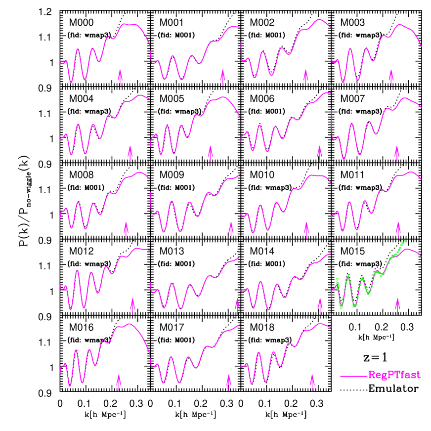
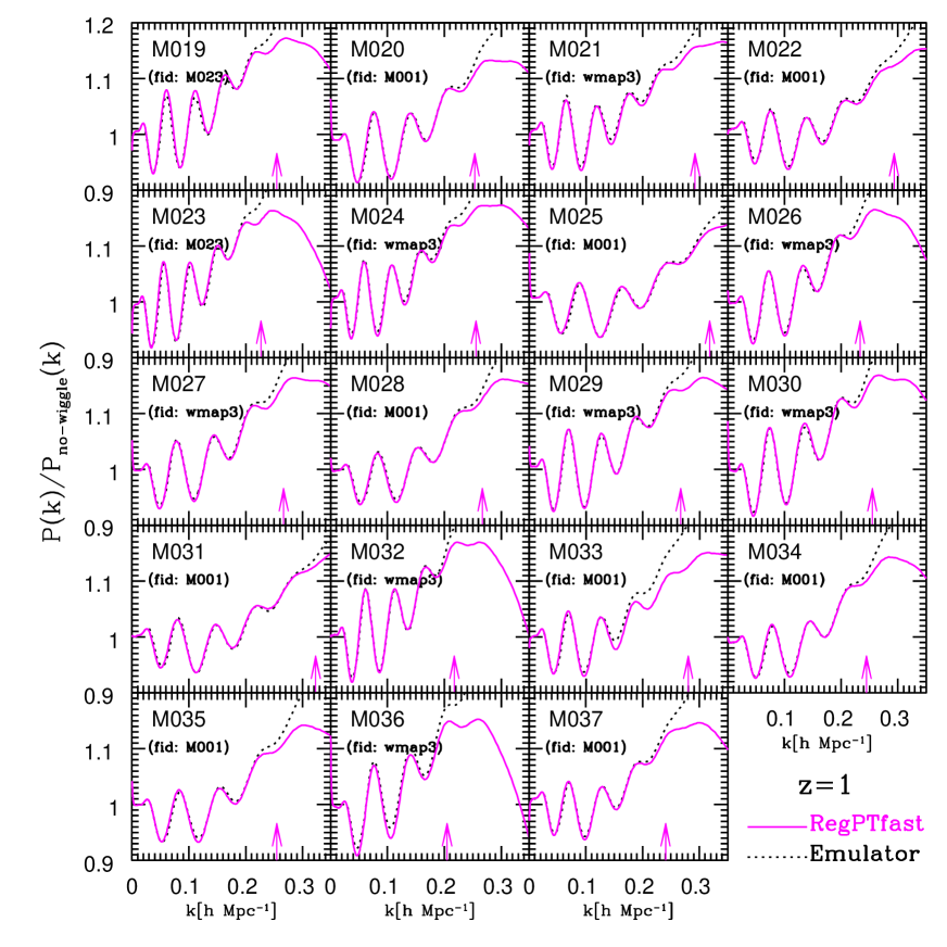
It is now time to discuss the accuracy of the overall RegPT scheme with general cosmic emulator predictions. Figs. 14 and 15 summarize the results of the comparison for all $38$ models, where we plot the ratios of power spectra, $P(k)/P_{\rm no\mbox{-}wiggle}(k)$, at specific redshift $z=1$. In each panel, magenta solid and black dashed lines represent the results of RegPT-fast and the power spectrum emulator code, respectively. Also, the fiducial model used for the RegPT-fast calculation is indicated, together with the label of the cosmological model. The two results mostly coincide with each other, and are hardly distinguishable at $k\lesssim 0.2\,h$ Mpc^-1, where the linear theory prediction typically produces a $10\%$ error. At $k\gtrsim 0.2\,h$ Mpc^-1, the RegPT-fast results tend to deviate from the predictions of the emulator code which probably indicates the the limitation of PT treatment. However, some models still show a remarkable agreement at $k\lesssim 0.3\,h$ Mpc^-1 (e.g., M009 and M013).

As the range of applicability of the RegPT scheme depend on both $k$ and the power spectrum amplitude, following Refs. Nishimichi et al. (2009); Taruya et al. (2009), we propose here a phenomenological rule for the domain of applicability of the RegPT  calculations. The proposed upper value for $k$ is $k_{\rm crit}$ that can be obtained from the implicit equation,

$$\frac{k_{\rm crit}^{2}}{6\pi^{2}}\int_{0}^{k_{\rm crit}}dq\,P_{\rm lin}(q;z)=C,$$ (49)

where $C$ is a fixed constant, $C=0.7$. The resulting values are depicted as vertical arrows in Figs. 14 and 15. Below the critical wavenumber, the RegPT scheme indeed agrees with results of the emulator code, mostly within a percent-level precision. We have also checked that this is also the case for $z=0.5$ with this definition of $k_{\rm crit.}$.

The RegPT scheme is therefore shown to give a fairly accurate prediction for the power spectrum in the weakly non-linear regime in the sense given above. RegPT direct calculations, or (almost) equivalently, RegPT-fast calculations with the three fiducial models we prepared, can be applied to a wide range of cosmological models. Though we did not discuss it here, we expect the same to be also true for the correlation function. Finally we note that as the relevant scale of weakly non-linear regime grows wider for higher redshifts, the applicability and reliability of the RegPT scheme is naturally enhanced. On the other hand, the emulation schemes to build up interpolated results from large sets of $N$-body simulations are generally efficient in predicting the power spectrum at non-linear scales but are more likely to fail at high-$z$, since the requirement for the force resolution in $N$-body simulation becomes more and more severe. In this respect, perturbative reconstruction schemes such as RegPT – but this would also be the case of mptbreeze – are complementary to $N$-body based predictions.

VII Conclusion

It is needless to say that future cosmological observations make the development of cosmological tool aiming at accurately predicting the large-scale statistical properties of the universe highly desirable. In the first part of the present paper, based on a renormalized perturbation theory (PT), we introduced an explicit computation scheme applied to the matter power spectrum and correlation function in weakly non-linear regime that consistently includes the PT corrections up to the two-loop order. The construction of the full expression for the power spectrum is based on the $\Gamma$-expansion, i.e. makes use of the multi-point propagators which are properly regularized so as to recover their expected resummed behavior at high-$k$ and to match the standard PT result at low-$k$. We call this regularized PT treatment RegPT. We have shown that the RegPT scheme provides an accurate prediction for both the power spectrum and the correlation function, leading to a percent-level agreement with $N$-body simulations in the weakly non-linear regime.

In the second half of the paper, we presented a method to accelerate the power spectrum calculations. The method utilizes prepared data sets for some specific fiducial models from which regularized PT calculations can be performed for arbitrary cosmological models. The main interest of this method is that the evaluation the residual PT corrections between fiducial and target cosmological models can be reduced to mere one-dimensional integrals. This enables us to dramatically reduce the computational cost, and even with single-node calculation by a laptop computer, the power spectrum calculation can be done in a few seconds. We call this method RegPT-fast, and we have demonstrated that the RegPT-fast treatment can perfectly reproduce the direct RegPT calculations that involve several multi-dimensional integrals.

We then investigated the range of applicability of the RegPT schemes in a broad class of cosmological models. For this purpose, we select 38 cosmological models, and compared the RegPT predictions – eventually incorporating the accelerated computations – with results of a power spectrum emulator code, cosmic emulator. We show that with the help of three fiducial models the RegPT-fast calculations give reliable predictions for the power spectra over this range of cosmological models. We furthermore put forward an empirical criterion (49) that gives a good indication of the applicable range of the RegPT scheme in $k$. The RegPT-fast treatment, together with the direct RegPT calculation, has been implemented in a fortran code that we publicly release as part of this paper.

Although this paper is focused on precision calculations of the matter power spectrum, the RegPT framework as well as the methodology for accelerated calculation can naturally be applied to the power spectrum of the velocity divergence and the cross-power spectrum of velocity and density fields in a similar way. The analysis of the velocity power spectrum, together with a detailed comparison with $N$-body simulations, will be presented elsewhere. Of particular interest is the application of the RegPT schemes to the redshift-space power spectrum or correlation function. In this case, not only the velocity and density power spectra, but also the multi-point spectra like bispectrum, arising from the non-linear mode coupling, seem to play important roles, and should be properly modeled. Significance of the effect of multi-point spectra has been recently advocated by Refs. Reid and White (2009); Taruya et al. (2010); Nishimichi and Taruya (2011); Tang et al. (2011), and there appear physical models that account for this. Combination of these models with the RegPT schemes would be very important, and we will discuss it in a near future.

Appendix A Perturbative reconstruction of RegPT  power spectrum at two-loop order

In this Appendix, we present the set of perturbative expressions that are used for the accelerated power spectrum calculation at two-loop order which is implemented in the RegPT-fast code.

In a similar manner to the one-loop case described in Sec. V.1, we can expand the power spectrum expression up to two-loop order around the fiducial cosmological model, and obtain the perturbative expression for power spectrum in the target cosmological model. Plugging Eq. (41) into the two-loop expression (30) and assuming $\delta P_{0}\ll P_{0,{\rm fid}}$, the power spectrum is written like (42), and the correction $P_{\rm corr}$ becomes

$$P_{\rm corr}[k,\eta,\sigma_{\rm d,target};\delta P_{0}(k)]=2\Gamma_{\rm reg}^{(1)}(k;\eta)\,\delta\Gamma_{\rm reg}^{(1)}(k;\eta)\,P_{0}(k)+\left[\Gamma_{\rm reg}^{(1)}(k;\eta)\right]^{2}\,\delta P_{0}(k)$$

$$\qquad+4\int\frac{d^{3}\mbox{\boldmath$q$}}{(2\pi)^{3}}\,\left\{\left[\Gamma_{\rm reg}^{(2)}(\mbox{\boldmath$q$},\mbox{\boldmath$k$}-\mbox{\boldmath$q$};\eta)\right]^{2}P_{0}(|\mbox{\boldmath$k$}-\mbox{\boldmath$q$}|)\,\delta P_{0}(q)+\Gamma_{\rm reg}^{(2)}(\mbox{\boldmath$q$},\mbox{\boldmath$k$}-\mbox{\boldmath$q$};\eta)\,\delta\Gamma_{\rm reg}^{(2)}(\mbox{\boldmath$q$},\mbox{\boldmath$k$}-\mbox{\boldmath$q$};\eta)\,P_{0}(|\mbox{\boldmath$k$}-\mbox{\boldmath$q$}|)\,P_{0}(q)\right\}$$

$$\qquad+18\int\frac{d^{3}\mbox{\boldmath$p$}d^{3}\mbox{\boldmath$q$}}{(2\pi)^{6}}\,\left[\Gamma_{\rm reg}^{(3)}(\mbox{\boldmath$p$},\mbox{\boldmath$q$},\mbox{\boldmath$k$}-\mbox{\boldmath$p$}-\mbox{\boldmath$q$};\eta)\right]^{2}P_{0}(|\mbox{\boldmath$k$}-\mbox{\boldmath$p$}-\mbox{\boldmath$q$}|)\,P_{0}(p)\,\delta P_{0}(q).$$ (50)

In the above, the perturbations of regularized propagators, $\delta\Gamma_{\rm reg}^{(1)}$ and $\delta\Gamma_{\rm reg}^{(2)}$, are described as

$$\delta\Gamma_{\rm reg}^{(1)}(k;\eta)=e^{3\eta}\left[(1+\alpha_{k})\,\delta\overline{\Gamma}^{(1)}_{\rm 1\mbox{-}loop}(k)+e^{2\eta}\,\delta\overline{\Gamma}^{(1)}_{\rm 2\mbox{-}loop}(k)\right]$$

$$\qquad\qquad\quad\times e^{-\alpha_{k}},$$ (51)

$$\delta\Gamma_{\rm reg}^{(2)}(\mbox{\boldmath$q$},\mbox{\boldmath$k$}-\mbox{\boldmath$q$};\eta)=e^{4\eta}\,\delta\overline{\Gamma}^{(2)}_{\rm 1\mbox{-}loop}(\mbox{\boldmath$q$},\mbox{\boldmath$k$}-\mbox{\boldmath$q$})\,e^{-\alpha_{k}},$$ (52)

where we define $\alpha_{k}\equiv k^{2}\sigma_{\rm d,target}^{2}e^{2\eta}/2$. The quantities $\delta\overline{\Gamma}^{(p)}_{\rm n\mbox{-}loop}$ are defined by

$$\delta\overline{\Gamma}^{(1)}_{\rm 1\mbox{-}loop}(k)=3\,\int\frac{d^{3}\mbox{\boldmath$q$}}{(2\pi)^{3}}\,F_{\rm sym}^{(3)}(\mbox{\boldmath$q$},-\mbox{\boldmath$q$},\mbox{\boldmath$k$})\,\delta P_{0}(q),$$ (53)

$$\delta\overline{\Gamma}^{(1)}_{\rm 2\mbox{-}loop}(k)=30\,\int\frac{d^{3}\mbox{\boldmath$q$}_{1}d^{3}\mbox{\boldmath$q$}_{2}}{(2\pi)^{6}}\,F_{\rm sym}^{(5)}(\mbox{\boldmath$q$}_{1},-\mbox{\boldmath$q$}_{1},\mbox{\boldmath$q$}_{2},-\mbox{\boldmath$q$}_{2},\mbox{\boldmath$k$})$$

$$\qquad\qquad\qquad\quad\times P_{0,{\rm fid}}(q_{1})\,\delta P_{0}(q_{2}),$$ (54)

$$\delta\overline{\Gamma}^{(2)}_{\rm 1\mbox{-}loop}(\mbox{\boldmath$k$}_{1},\mbox{\boldmath$k$}_{2})=6\int\frac{d^{3}\mbox{\boldmath$q$}}{(2\pi)^{3}}\,F_{\rm sym}^{(4)}(\mbox{\boldmath$q$},-\mbox{\boldmath$q$},\mbox{\boldmath$k$}_{1},\mbox{\boldmath$k$}_{2})\,\delta P_{0}(q).$$ (55)

The kernels $F_{\rm sym}^{(p)}$ are the symmetrized standard PT kernel for density field. In the above, the angular integrals are known to be analytically performed (Refs. Crocce and Scoccimarro (2006b); Bernardeau et al. (2012b), and Bernardeau et al. in prep.), one may write

$$\delta\overline{\Gamma}^{(1)}_{\rm 1\mbox{-}loop}(k)=\int\frac{dq\,q^{2}}{2\pi^{2}}\,f(q;k)\,\delta P_{0}(q),$$ (56)

$$\delta\overline{\Gamma}^{(1)}_{\rm 2\mbox{-}loop}(k)=2\,\int\frac{dq_{1}\,dq_{2}\,\,q_{1}^{2}\,q_{2}^{2}}{(2\pi^{2})^{2}}\,J(q_{1},q_{2};k)$$

$$\qquad\qquad\qquad\qquad\qquad\times P_{0,{\rm fid}}(q_{1})\,\delta P_{0}(q_{2}),$$ (57)

$$\delta\overline{\Gamma}^{(2)}_{\rm 1\mbox{-}loop}(\mbox{\boldmath$k$}_{1},\mbox{\boldmath$k$}_{2})=\int\frac{dq}{2\pi^{2}}\,K(q;k_{1},k_{2},k_{3})\,\delta P_{0}(q)$$ (58)

with the angle-averaged kernels $f$, $J$ and $K$ defined by

$$f(q;k)=3\int\frac{d^{2}\mbox{\boldmath$\Omega$}_{q}}{4\pi}\,F_{\rm sym}^{(3)}(\mbox{\boldmath$q$},-\mbox{\boldmath$q$},\mbox{\boldmath$k$}),$$ (59)

$$J(q_{1},q_{2};k)=15\,\int\frac{d^{2}\mbox{\boldmath$\Omega$}_{q_{1}}\,d^{2}\mbox{\boldmath$\Omega$}_{q_{2}}}{(4\pi)^{2}}\,$$

$$\qquad\qquad\qquad\qquad\times F_{\rm sym}^{(5)}(\mbox{\boldmath$q$}_{1},-\mbox{\boldmath$q$}_{1},\mbox{\boldmath$q$}_{2},-\mbox{\boldmath$q$}_{2},\mbox{\boldmath$k$}),$$ (60)

$$K(q;k_{1},k_{2},k_{3})=6\,\int\frac{d^{2}\mbox{\boldmath$\Omega$}_{q}}{4\pi}\,F_{\rm sym}^{(4)}(\mbox{\boldmath$q$},-\mbox{\boldmath$q$},\mbox{\boldmath$k$}_{1},\mbox{\boldmath$k$}_{2}).$$ (61)

Note that $\mbox{\boldmath$k$}_{1}+\mbox{\boldmath$k$}_{2}=\mbox{\boldmath$k$}_{3}$.

The expression for the correction $P_{\rm corr}$ given above contains many integrals involving the perturbed linear power spectrum, $\delta P_{0}$, and some of these require multi-dimensional integrals. However, those multi-dimensional integration are separately treated, and can be effectively reduced to the one-dimensional integrals as follows,

$$\delta\overline{\Gamma}_{\rm 1\mbox{-}loop}^{(1)}(k)=\int\frac{dqq^{2}}{2\pi^{2}}L^{(1)}(q,k)\,\delta P_{0}(q),$$ (62)

$$\delta\overline{\Gamma}_{\rm 2\mbox{-}loop}^{(1)}(k)=2\int\frac{dqq^{2}}{2\pi^{2}}M^{(1)}(q,k)\,\delta P_{0}(q),$$ (63)

$$\int\frac{d^{3}\mbox{\boldmath$q$}d^{3}\mbox{\boldmath$q$}}{(2\pi)^{3}}\left[\Gamma_{\rm reg}^{(2)}(\mbox{\boldmath$q$},\mbox{\boldmath$k$}-\mbox{\boldmath$q$};\eta)\right]^{2}P_{0,{\rm fid}}(|\mbox{\boldmath$k$}-\mbox{\boldmath$q$}|)\,\delta P_{0}(q)=e^{4\eta}\Bigl{[}\left(1+\alpha_{k}\right)^{2}\int\frac{dq\,q^{2}}{2\pi^{2}}X^{(2)}(q,k)\,\delta P_{0}(q)$$

$$\qquad\qquad+2e^{2\eta}\,\left(1+\alpha_{k}\right)\int\frac{dq\,q^{2}}{2\pi^{2}}Y^{(2)}(q,k)\,\delta P_{0}(q)+e^{4\eta}\,\int\frac{dq\,q^{2}}{2\pi^{2}}Z^{(2)}(q,k)\,\delta P_{0}(q)\Bigr{]}\exp\left\{-2\alpha_{k}\right\},$$ (64)

$$\int\frac{d^{3}\mbox{\boldmath$q$}}{(2\pi)^{3}}\,\Gamma_{\rm reg}^{(2)}(\mbox{\boldmath$q$},\mbox{\boldmath$k$}-\mbox{\boldmath$q$};\eta)\,\delta\Gamma_{\rm reg}^{(2)}(\mbox{\boldmath$q$},\mbox{\boldmath$k$}-\mbox{\boldmath$q$};\eta)\,P_{0,{\rm fid}}(|\mbox{\boldmath$k$}-\mbox{\boldmath$q$}|)P_{0,{\rm fid}}(q)$$

$$\qquad=e^{6\eta}\Bigl{[}(1+\alpha_{k})\,\int\frac{dpp^{2}}{2\pi^{2}}\,Q^{(2)}(p,k)\,\delta P_{0}(p)+e^{2\eta}\,\int\frac{dpp^{2}}{2\pi^{2}}\,R^{(2)}(p,k)\,\delta P_{0}(p)\Bigr{]}e^{-2\alpha_{k}},$$ (65)

$$\int\frac{d^{3}\mbox{\boldmath$q$}d^{3}\mbox{\boldmath$q$}}{(2\pi)^{6}}\left[\Gamma_{\rm reg}^{(3)}(\mbox{\boldmath$p$},\mbox{\boldmath$q$},\mbox{\boldmath$k$}-\mbox{\boldmath$p$}-bfq;\eta)\right]^{2}\,P_{0,{\rm fid}}(|\mbox{\boldmath$k$}-\mbox{\boldmath$p$}-\mbox{\boldmath$q$}|)P_{0,{\rm fid}}(p)\,\delta P_{0}(q)=e^{6\eta}\,e^{-2\alpha_{k}}\,\int\frac{dq\,q^{2}}{2\pi^{2}}\,S^{(3)}(q,k)\,\delta P_{0}(q).$$ (66)

In the above, the kernels of the integrals, $L$, $M$, $X$, $Y$, $Z$, $Q$, $R$, and $S$, additionally need to be computed, but we only have to evaluate them once for each fiducial cosmological model,

$$L^{(1)}(q,k)=f(q;k),$$ (67)

$$M^{(1)}(q,k)=\int\frac{dp\,p^{2}}{2\pi^{2}}J(p,q;k)\,P_{0,{\rm fid}}(p),$$ (68)

$$X^{(2)}(q,k)=\frac{1}{2}\int_{-1}^{1}d\mu_{q}\,\left[F^{(2)}_{\rm sym}(\mbox{\boldmath$q$},\mbox{\boldmath$k$}-\mbox{\boldmath$q$})\right]^{2}\,P_{0,{\rm fid}}(\sqrt{k^{2}-2kq\,\mu_{q}+q^{2}}),$$ (69)

$$Y^{(2)}(q,k)=\frac{1}{2}\int_{-1}^{1}d\mu_{q}\,F^{(2)}_{\rm sym}(\mbox{\boldmath$q$},\mbox{\boldmath$k$}-\mbox{\boldmath$q$})\,\overline{\Gamma}^{(2)}_{\rm 1\mbox{-}loop}(\mbox{\boldmath$q$},\mbox{\boldmath$k$}-\mbox{\boldmath$q$})\,P_{0,{\rm fid}}(\sqrt{k^{2}-2kq\,\mu_{q}+q^{2}}),$$ (70)

$$Z^{(2)}(q,k)=\frac{1}{2}\int_{-1}^{1}d\mu_{q}\,\left[\overline{\Gamma}^{(2)}_{\rm 1\mbox{-}loop}(\mbox{\boldmath$q$},\mbox{\boldmath$k$}-\mbox{\boldmath$q$})\right]^{2}\,P_{0,{\rm fid}}(\sqrt{k^{2}-2kq\,\mu_{q}+q^{2}}),$$ (71)

$$Q^{(2)}(p,k)=\int\frac{d^{3}\mbox{\boldmath$q$}}{(2\pi)^{3}}F^{(2)}_{\rm sym}(\mbox{\boldmath$q$},\mbox{\boldmath$k$}-\mbox{\boldmath$q$})\,K(p:q,|\mbox{\boldmath$k$}-\mbox{\boldmath$q$}|,k)\,P_{0,{\rm fid}}(|\mbox{\boldmath$k$}-\mbox{\boldmath$q$}|)\,P_{0,{\rm fid}}(q),$$ (72)

$$R^{(2)}(p,k)=\int\frac{d^{3}\mbox{\boldmath$q$}}{(2\pi)^{3}}\overline{\Gamma}^{(2)}_{\rm 1\mbox{-}loop}(\mbox{\boldmath$q$},\mbox{\boldmath$k$}-\mbox{\boldmath$q$})\,K(p;q,|\mbox{\boldmath$k$}-\mbox{\boldmath$q$}|,k)\,P_{0,{\rm fid}}(|\mbox{\boldmath$k$}-\mbox{\boldmath$q$}|)\,P_{0,{\rm fid}}(q),$$ (73)

$$S^{(3)}(q,k)=\frac{1}{2}\int_{-1}^{1}d\mu_{q}\,\int\frac{d^{3}\mbox{\boldmath$p$}}{(2\pi)^{3}}\left[F^{(3)}_{\rm sym}(\mbox{\boldmath$p$},\mbox{\boldmath$q$},\mbox{\boldmath$k$}-\mbox{\boldmath$p$}-\mbox{\boldmath$q$})\right]^{2}\,P_{0,{\rm fid}}(|\mbox{\boldmath$k$}-\mbox{\boldmath$p$}-\mbox{\boldmath$q$}|)\,P_{0,{\rm fid}}(p),$$ (74)

with the variable $\mu_{q}$ defined by $\mu_{q}=(\mbox{\boldmath$k$}\cdot\mbox{\boldmath$q$})/(k\,q)$.

Note that similar to the one-loop case, the correction at two-loop order also possesses a one-parameter degree of freedom corresponding to a re-scaling the power spectrum amplitude of fiducial model, $P_{0,{\rm fid}}\to c\,P_{0,{\rm fid}}$. The power spectrum difference $\delta P_{0}$ can then be made small securing the rapid convergence of this expansion.

Finally, the data set of kernel functions given above are supplemented in the RegPT code, with $301\times 301$ logarithmic arrays in $(k,q)$ space. For specific three fiducial models (i.e., wmap3, M001, and M023), the data have been obtained using the method of Gaussian quadrature up to three-dimensional integrals and Monte Carlo technique for four-dimensional integral. Together with un-perturbed part of the PT corrections, these can be used as fast calculations of power spectrum at two-loop order.

Appendix B Code description

In this Appendix, we present a detailed description of the fortran code, RegPT, which computes the power spectrum and correlation function of density fields valid at weakly non-linear regime of gravitational clustering.

B.1 Overview

The code, RegPT, is compiled with the fortran compilers, ifort or gfortran. It computes the power spectrum in flat wCDM class models based on the RegPT treatment when provided with either of transfer function or matter power spectrum. It then gives the multiple-redshift outputs for power spectrum, and optionally provides correlation function data. We have implemented two major options for power spectrum calculations:

• -fast: Applying the reconstruction method described in Sec. V.1, this option quickly computes the power spectrum at two-loop level (typically a few seconds), using the pre-computed data set of PT kernels for fiducial cosmological models. We provide the data set for three fiducial models (wmap3, M001, and M023, see Table 2), and the code automatically finds an appropriate fiducial model to closely match the result of rigorous PT calculation with direct-mode.

• -direct: With this option, the code first applies the fast method, and then follows the regularized expression for power spectrum (see Eq.[30] with regularized propagators [31]-[33]) to directly evaluate the multi-dimensional integrals (it typically takes a few minutes). The output results are the power spectrum of direct calculation and difference of the results between fast and direct method. Further, the code gives the data set of PT diagrams necessary for power spectrum calculations, from which we can construct the power spectrum. We provide a supplemental code, read_stfile.f, with which the power spectrum and correlation function can be evaluated from the diagram data set in several PT methods, including the standard PT and Lagrangian resummation theory (LRT) Matsubara (2008a); Okamura et al. (2011) as well as RegPT treatment (see Appendix B.4.3).

In addition, the code supports the option, -direct1loop, to compute the power spectrum at one-loop order. Although this is based on the direct calculation with multi-dimensional integration (see Eq. [37] with regularized propagators [38][39]), the one-loop expression involves two-dimensional integrals at most, and thus the computational cost is less expensive. It is potentially useful for the computation of high-$z$ correlation function and power spectrum.

B.2 Setup

The RegPT code is available at http://www-utap.phys.s.u-tokyo.ac.jp/~ataruya/regpt_code.html A part of RegPT code uses the library for Monte Carlo integration, CUBA Hahn (2005). Before compiling the codes, users should download the library package cuba-1.5, and correctly build the file, libcuba.a, compatible with the architecture of user’s platform. This can be done in the directory /Cuba-1.5, and just type ./configure and make lib. After placing the library file libcuba.a at the directory /RegPT/src, users can use the Makefile to create the main executable file, RegPT.exe. Note that currently available compilers are intel fortran compiler, ifort, and GNU fortran compiler, gfortran.

B.3 Running the code

Provided with linear power spectrum or transfer function data, the code runs with a set of options, and computes power spectrum. Users can specify the options in the command line, or using the parameter file (suffix of file name should be .ini). Sample of parameter file is supplied in the code (see directory /RegPT/example).

For running the code with the command-line options, a simple example is (assuming the code is placed at the directory, /RegPT)

./RegPT.exe -spectrum -infile matterpower_wmap5.dat -nz 2 0.5 1.0

In the above example, the code first reads the input data file, matterpower_wmap5.dat, which is assumed to contain linear power spectrum data consisting of two columns, i.e., $k$ and $P_{0}(k)$. By default setting, fast mode is chosen, and the output result of power spectrum is saved to pk_RegPT.dat. With the option -nz 2 0.5 1.0, the output file contains the power spectrum results at two redshifts, $z=0.5$ and $1.0$ (see Appendix B.4.1 for output format). Note that by default, the code adopts specific values of cosmological parameters. Making use of options, users can change the value of cosmological parameters appropriately, consistently with input power spectrum (or transfer function) data.

Here we summarize the available options to run the code:

• Verbose level for output message

  -verbose   $n$: This sets the verbose level for output information on the progress of numerical computation. The available level $n$ is 1 or 2 (default: -verbose 1).

  -noverbose: This option suppresses the message while running the code.

• Input data file

  -infile   [ file ]: Input file name of power spectrum or transfer function data is specified (default: -infile matterpower.dat).

  -path   [ path to input file ]: This specifies the path to the input file (default: -path ./).

  -spectrum: With this option, the code assumes that the input file is power spectrum data. The data consists of two columns, i.e., wavenumber (in units of $h\,$Mpc^-1) and matter power spectrum (in units of $h^{-3}$ Mpc³) (default: -spectrum). The normalization of power spectrum amplitude can be made with the option -sigma8.

  -transfer: With this option, the code assumes that the input file is the transfer function data created by CAMB. The data should contain $7$ columns, among which the code uses the first and seven columns (wavenumber in units of $h\,$Mpc^-1 and matter transfer function). The normalization of power spectrum amplitude can be made with either of the option -sigma8 or -samp and -spivot.

• Specification of cosmological parameters

  -sigma8   $\sigma_{8}$: This option sets the power spectrum normalization by $\sigma_{8}$ (default: -sigma8 0.817). For $\sigma_{8}<0$, the code will skip the $\sigma_{8}$ normalization.

  -samp   $A_{\rm s}$: This option sets the amplitude of power spectrum at pivot scale $k_{\rm pivot}$ (default: -samp 2.1e-9). This option is used for normalization of transfer function data, and is valid when the option -transfer is specified.

  -spivot   $k_{\rm pivot}$: This option sets the pivot scale of CMB normalization in units of Mpc^-1 (default: -spivot 0.05). This option is used for normalization of transfer function data, and is valid when the option -transfer is specified.

  -omegam   $\Omega_{\rm m}$: This option sets the mass density parameter (default: -omegam 0.279). This is used to estimate the linear growth factor and to compute the smooth reference spectrum, $P_{\rm no\mbox{-}wiggle}(k)$.

  -omegab   $\Omega_{\rm b}$: This option sets the baryon density parameter (default: -omegab 0.165*omegam). This is used to compute the smooth reference spectrum, $P_{\rm no\mbox{-}wiggle}(k)$.

  -ns   $n_{\rm s}$: This option sets the scalar spectral index. This is used to compute the linear power spectrum from the transfer function data (option -transfer should be specified), and to compute the smooth reference spectrum, $P_{\rm no\mbox{-}wiggle}(k)$.

  -w   $w$: This option sets the equation of state for dark energy (default: -w -1.0). This is used to estimate the linear growth factor.

  -h   $h$: This option sets the Hubble parameter (default: -h 0.701). This is used to compute the power spectrum from the transfer function data, and to compute the smooth reference spectrum, $P_{\rm no\mbox{-}wiggle}(k)$.

  -camb   [ output parameter file of camb ]: With this option, the code reads the CAMB output parameter file, and specifies the cosmological parameters ($\Omega_{\rm m}$, $\Omega_{\rm b}$, $w$, $h$, $n_{\rm s}$, $A_{\rm s}$, $k_{\rm pivot}$).

• Calculation mode of RegPT

  -fast: This option adopts the fast method of power spectrum calculation to give RegPT results. This is default setting.

  -direct: This option first applies the fast method, and then follow the direct method for RegPT calculation.

  -direct1loop: With this option, the code adopts direct method to compute the power spectrum at one-loop order.

• Setup of fiducial models for fast- and direct-mode calculations

  -datapath   [ path to data directory ]: This option specifies the path to the data files used for power spectrum calculation with fast and direct methods (default: -datapath data/). In the directory specified with this option, the data set of kernel functions given in Appendix A and un-perturbed part of power spectrum corrections, as well as the matter power spectrum should be stored for three fiducial cosmological models (wmap3, M001, M023).

  -fiducial   [ model ]: This option sets the specific fiducial model among the three, wmap3, M001, and M023 (in default setting, the code automatically selects an appropriate fiducial model).

• Output data file

  -xicompute: With this option, the code computes the correlation function after power spectrum calculations, and creates the output file.

  -nz   $n$  $z_{1}\,\,\cdots\,\,z_{n}$: This option specifies the output redshifts for power spectrum calculations. The integer $n$ specifies the number of redshifts, and subsequent arguments specify the value of each redshift (default: -nz 1 1.0).

  -pkfile   [ file ]: This option sets the output file name of power spectrum data (default: pk_RegPT.dat).

  -xifile   [ file ]: This option sets the output file name of correlation function data (default: xi_RegPT.dat).

  -stfile   [ file ]: This option sets the output file name of PT diagram data (default: st_PT.dat).

B.4 Output file format

In what follows, wavenumber $k$ and separation $r$ are in units of $h\,$Mpc^-1 and $h^{-1}\,$Mpc, respectively. All the power spectrum data are assumed to be in units of $h^{-3}\,$Mpc³.

B.4.1 Power spectrum data

By default, RegPT code creates the output file for the power spectrum data (default file name is pk_RegPT.dat). The columns of this file include

$$k,\,\,\mbox{[data for $z_{1}$]},\,\,\mbox{[data for $z_{2}$]},\,\,\cdots,\mbox{[data for $z_{n}$]}$$

The first column is the wavenumber, while the bracket [data for $z_{i}$] represents a set of power spectra at given redshift $z_{i}$ and wavenumber $k$. Number of the data set is specified with the option -nz, and each data contains

$$P_{\rm no\mbox{-}wiggle}(k,z_{i}),\,\,P_{\rm lin}(k,z_{i}),\,\,P_{\rm RegPT}(k,z_{i}),\,\,\mbox{Err}(k)$$

Here, the spectrum $P_{\rm no\mbox{-}wiggle}$ is the smooth reference spectrum calculated from the no-wiggle formula of linear transfer function in Ref. Eisenstein and Hu (1998), $P_{\rm lin}$ is the linearly extrapolated spectrum, and $P_{\rm RegPT}(k,z_{i})$ represents the power spectrum based on the RegPT calculations with fast and/or direct method (depending on the choice of options, -fast, -direct or -direct1loop). The last column, Err, usually sets to zero, but with the option -direct, it gives the difference of the power spectra between fast and direct methods.

B.4.2 Correlation function data

With the option -xicompute, the code also provides the output file for correlation function data (default file name is xi_RegPT.dat). Similar to the power spectrum data, the structure of the data is

$$r,\,\,\mbox{[data for $z_{1}$]},\,\,\mbox{[data for $z_{2}$]},\,\,\cdots,\mbox{[data for $z_{n}$]}$$

The first column is the separation, while the bracket [data for $z_{i}$] represents a set of correlation functions given at redshift $z_{i}$ and separation $r$, containing two columns:

$$\xi_{\rm lin}(r,z_{i}),\,\,\xi_{\rm RegPT}(r,z_{i})$$

These are simply obtained from the output results of power spectrum based on the expression (36). Note that the range of wavenumber for output power spectrum is restricted to the wavenumber coverage of input linear spectrum (or transfer function). To get a convergent result of correlation functions, users may have to supply the input data file with a sufficiently wide range of wavenumber (e.g., $10^{-3}\leq k\leq 10$ $h\,$Mpc^-1).

B.4.3 Diagram data

When users specifies the -direct option, the code additionally provides a set of PT diagram data necessary for power spectrum computation, from which we can construct the power spectrum at one- and two-loop order. The output file (default file name is st_PT.dat) includes the following columns:

$$k,\,\,P_{\rm no\mbox{-}wiggle}(k),\,\,P_{\rm lin}(k),\,\,\overline{\Gamma}^{(1)}_{1\mbox{-}{\rm loop}}(k),\,\,\overline{\Gamma}^{(1)}_{2\mbox{-}{\rm loop}}(k),\,\,P_{\rm corr}^{(2){\rm tree\mbox{-}tree}}(k),\,\,P_{\rm corr}^{(2){\rm tree\mbox{-}1loop}}(k),\,\,P_{\rm corr}^{(2){\rm 1loop\mbox{-}1loop}}(k),\,\,P_{\rm corr}^{(3){\rm tree\mbox{-}tree}}(k)$$

Here, the power spectra $P_{\rm no\mbox{-}wiggle}$ and $P_{\rm lin}$ are basically the same data as contained in the power spectrum file, but these are the extrapolated data at $z=0$ (that is, $P_{\rm lin}$ corresponds to $P_{0}$). The function $\overline{\Gamma}^{(1)}_{n\mbox{-}{\rm loop}}$ is the two-point propagator of the standard PT expansion (see definition [26]). The functions in the remaining four columns, $P_{\rm corr}^{(2){\rm tree\mbox{-}tree}}$, $P_{\rm corr}^{(2){\rm tree\mbox{-}1loop}}$, $P_{\rm corr}^{(2){\rm 1loop\mbox{-}1loop}}$, and $P_{\rm corr}^{(3){\rm tree\mbox{-}tree}}$, are defined by

$$P^{(2)\rm tree\mbox{-}tree}_{\rm corr}(k)=2\int\frac{d^{3}\mbox{\boldmath$q$}}{(2\pi)^{3}}F_{\rm sym}^{(2)}(\mbox{\boldmath$q$},\mbox{\boldmath$k$}-\mbox{\boldmath$q$})F_{\rm sym}^{(2)}(\mbox{\boldmath$q$},\mbox{\boldmath$k$}-\mbox{\boldmath$q$})P_{0}(q)P_{0}(|\mbox{\boldmath$k$}-\mbox{\boldmath$q$}|),$$ (75)

$$P^{(2)\rm tree\mbox{-}1loop}_{\rm corr}(k)=4\int\frac{d^{3}\mbox{\boldmath$q$}}{(2\pi)^{3}}F_{\rm sym}^{(2)}(\mbox{\boldmath$q$},\mbox{\boldmath$k$}-\mbox{\boldmath$q$})\overline{\Gamma}_{\rm 1\mbox{-}loop}^{(2)}(\mbox{\boldmath$q$},\mbox{\boldmath$k$}-\mbox{\boldmath$q$})P_{0}(q)P_{0}(|\mbox{\boldmath$k$}-\mbox{\boldmath$q$}|),$$ (76)

$$P^{(2)\rm 1loop\mbox{-}1loop}_{\rm corr}(k)=2\int\frac{d^{3}\mbox{\boldmath$q$}}{(2\pi)^{3}}\overline{\Gamma}_{\rm 1\mbox{-}loop}^{(2)}(\mbox{\boldmath$q$},\mbox{\boldmath$k$}-\mbox{\boldmath$q$})\overline{\Gamma}_{\rm 1\mbox{-}loop}^{(2)}(\mbox{\boldmath$q$},\mbox{\boldmath$k$}-\mbox{\boldmath$q$})P_{0}(q)P_{0}(|\mbox{\boldmath$k$}-\mbox{\boldmath$q$}|),$$ (77)

$$P^{(3)\rm tree\mbox{-}tree}_{\rm corr}(k)=6\int\frac{d^{3}\mbox{\boldmath$p$}\,d^{3}\mbox{\boldmath$q$}}{(2\pi)^{6}}F^{(3)}_{\rm sym}(\mbox{\boldmath$p$},\mbox{\boldmath$q$},\mbox{\boldmath$k$}-\mbox{\boldmath$p$}-\mbox{\boldmath$q$})F^{(3)}_{\rm sym}(\mbox{\boldmath$p$},\mbox{\boldmath$q$},\mbox{\boldmath$k$}-\mbox{\boldmath$p$}-\mbox{\boldmath$q$})P_{0}(p)P_{0}(q)P_{0}(|\mbox{\boldmath$k$}-\mbox{\boldmath$p$}-\mbox{\boldmath$q$}|).$$ (78)

Provided the data set above, the power spectrum can be constructed with

$$P_{\rm 1\mbox{-}loop}^{\rm RegPT}(k;\eta)=e^{2\eta}\,e^{-2\alpha_{k}}\left[\left\{1+\alpha_{k}+e^{2\eta}\,\overline{\Gamma}_{\rm 1\mbox{-}loop}^{(1)}(k)\right\}^{2}\,P_{0}(k)+e^{2\eta}\,P^{(2)\rm tree\mbox{-}tree}_{\rm corr}(k)\right],$$ (79)

$$P_{\rm 2\mbox{-}loop}^{\rm RegPT}(k;\eta)=e^{2\eta}\,e^{-2\alpha_{k}}\Bigl{[}\,\,\Bigl{\{}1+\alpha_{k}+\frac{\alpha_{k}^{2}}{2}+e^{2\eta}\,\overline{\Gamma}_{\rm 1\mbox{-}loop}^{(1)}(k)\left(1+\alpha_{k}\right)+e^{4\eta}\,\overline{\Gamma}_{\rm 2\mbox{-}loop}^{(1)}(k)\Bigr{\}}^{2}\,P_{0}(k)$$

$$\quad+e^{2\eta}\left\{(1+\alpha_{k})^{2}P^{(2)\rm tree\mbox{-}tree}_{\rm corr}(k)+e^{2\eta}(1+\alpha_{k})P^{(2)\rm tree\mbox{-}1loop}_{\rm corr}(k)+e^{4\eta}\,P^{(2)\rm 1loop\mbox{-}1loop}_{\rm corr}(k)\right\}+e^{4\eta}\,P^{(3)\rm 1loop\mbox{-}1loop}_{\rm corr}(k)\,\,\Bigr{]},$$ (80)

for the RegPT calculation at one- and two-loop order, respectively. Here, $\alpha_{k}$ is given by $\alpha_{k}=k^{2}\sigma_{\rm d}^{2}e^{2\eta}/2$ with $\sigma_{\rm d}$ being the dispersion of displacement field (see Eq. [23]). Note that the diagram data set can be also used to compute the power spectrum in the standard PT calculations:

$$P_{\rm 1\mbox{-}loop}^{\rm SPT}(k;\eta)=e^{2\eta}\,P_{0}(k)+e^{4\eta}\left[2\,P_{0}(k)\,\overline{\Gamma}_{1\mbox{-}{\rm loop}}^{(1)}(k)+P^{(2)\rm tree\mbox{-}tree}_{\rm corr}(k)\right],$$ (81)

$$P_{\rm 2\mbox{-}loop}^{\rm SPT}(k;\eta)=P_{\rm 1\mbox{-}loop}^{\rm SPT}(k;\eta)+e^{6\eta}\,\Bigl{[}\,\,P_{0}(k)\,\{\overline{\Gamma}_{1\mbox{-}{\rm loop}}^{(1)}(k)\}^{2}+P^{(3)\rm tree\mbox{-}tree}_{\rm corr}(k)+P^{(2)\rm tree\mbox{-}1loop}_{\rm corr}(k)+2P_{0}(k)\,\overline{\Gamma}_{2\mbox{-}{\rm loop}}^{(1)}(k)\Bigr{]}.$$ (82)

With the supplemental code, read_stfile.f, users can easily compute the power spectrum in both RegPT and standard PT treatments. The code also provides the power spectrum result for LRT Matsubara (2008a); Okamura et al. (2011). A brief instruction on how to run the code and the output format of data is described in the header of the code.

B.5 Limitation

Since the RegPT code is the PT-based calculation code valid at weakly non-linear scales, the applicability of the output results is restricted to a certain range of wavenumber in power spectrum. We provide an empirical estimate of critical wavenumber $k_{\rm crit}$, below which the RegPT results are reliable and their accuracy can reach a percent level. This is based on Eq. (49) with constant value $C=0.7\,(0.3)$ for two-loop (one-loop) (see Sec. VI.2). With the option -verbose 2, the code displays the critical wavenumbers at output redshifts. Note that the value $k_{\rm crit}$ given here is just a crude estimate, and the actual domain of applicability may be somewhat wider or narrower. Users should use the output results with a great care.

References

- Eisenstein et al. (2005) D. J. Eisenstein et al. (SDSS), Astrophys. J. 633, 560 (2005), eprint astro-ph/0501171.
- Percival et al. (2010) W. J. Percival et al., Mon. Not. Roy. Astron. Soc. 401, 2148 (2010), eprint 0907.1660.
- Blake et al. (2011a) C. Blake, T. Davis, G. Poole, D. Parkinson, S. Brough, et al., Mon.Not.Roy.Astron.Soc. 415, 2892 (2011a), eprint 1105.2862.
- Seo et al. (2012) H.-J. Seo, S. Ho, M. White, A. Cuesta, A. Ross, et al. (2012), eprint 1201.2172.
- Anderson et al. (2012) L. Anderson, E. Aubourg, S. Bailey, D. Bizyaev, M. Blanton, et al. (2012), eprint 1203.6594.
- Seo and Eisenstein (2003) H.-J. Seo and D. J. Eisenstein, Astrophys. J. 598, 720 (2003), eprint astro-ph/0307460.
- Blake and Glazebrook (2003) C. Blake and K. Glazebrook, Astrophys. J. 594, 665 (2003), eprint astro-ph/0301632.
- Glazebrook and Blake (2005) K. Glazebrook and C. Blake, Astrophys. J. 631, 1 (2005), eprint astro-ph/0505608.
- Shoji et al. (2009) M. Shoji, D. Jeong, and E. Komatsu, Astrophys. J. 693, 1404 (2009), eprint 0805.4238.
- Padmanabhan and White (2008) N. Padmanabhan and M. J. White, 1, Phys. Rev. D77, 123540 (2008), eprint 0804.0799.
- Linder (2008) E. V. Linder, Astropart. Phys. 29, 336 (2008), eprint 0709.1113.
- Guzzo et al. (2008) L. Guzzo et al., Nature 451, 541 (2008), eprint 0802.1944.
- Yamamoto et al. (2008) K. Yamamoto, T. Sato, and G. Huetsi, Prog. Theor. Phys. 120, 609 (2008), eprint 0805.4789.
- Song and Percival (2009) Y.-S. Song and W. J. Percival, JCAP 0910, 004 (2009), eprint 0807.0810.
- Blake et al. (2011b) C. Blake, S. Brough, M. Colless, C. Contreras, W. Couch, et al., Mon.Not.Roy.Astron.Soc. 415, 2876 (2011b), eprint 1104.2948.
- Van Waerbeke et al. (2000) L. Van Waerbeke, Y. Mellier, T. Erben, J. C. Cuillandre, F. Bernardeau, R. Maoli, E. Bertin, H. J. McCracken, O. Le Fèvre, B. Fort, et al., Astron. & Astrophys. 358, 30 (2000), eprint arXiv:astro-ph/0002500.
- Fu et al. (2008) L. Fu, E. Semboloni, H. Hoekstra, M. Kilbinger, L. van Waerbeke, I. Tereno, Y. Mellier, C. Heymans, J. Coupon, K. Benabed, et al., Astron. & Astrophys. 479, 9 (2008), eprint 0712.0884.
- Bartelmann and Schneider (2001) M. Bartelmann and P. Schneider, Phys. Rep. 340, 291 (2001), eprint arXiv:astro-ph/9912508.
- Van Waerbeke and Mellier (2003) L. Van Waerbeke and Y. Mellier, ArXiv Astrophysics e-prints (2003), eprint arXiv:astro-ph/0305089.
- Crocce and Scoccimarro (2006a) M. Crocce and R. Scoccimarro, Phys. Rev. D73, 063519 (2006a), eprint astro-ph/0509418.
- Carlson et al. (2009) J. Carlson, M. White, and N. Padmanabhan, Phys. Rev. D80, 043531 (2009), eprint 0905.0479.
- Taruya et al. (2009) A. Taruya, T. Nishimichi, S. Saito, and T. Hiramatsu, Phys. Rev. D80, 123503 (2009), eprint 0906.0507.
- Crocce and Scoccimarro (2006b) M. Crocce and R. Scoccimarro, Phys. Rev. D73, 063520 (2006b), eprint astro-ph/0509419.
- Crocce and Scoccimarro (2008) M. Crocce and R. Scoccimarro, Phys. Rev. D77, 023533 (2008), eprint 0704.2783.
- Matsubara (2008a) T. Matsubara, Phys. Rev. D77, 063530 (2008a), eprint 0711.2521.
- Matsubara (2008b) T. Matsubara, Phys. Rev. D78, 083519 (2008b), eprint 0807.1733.
- McDonald (2007) P. McDonald, Phys. Rev. D75, 043514 (2007), eprint astro-ph/0606028.
- Izumi and Soda (2007) K. Izumi and J. Soda, Phys. Rev. D76, 083517 (2007), eprint 0706.1604.
- Taruya and Hiramatsu (2008) A. Taruya and T. Hiramatsu, Astrophys.J. 674, 617 (2008), eprint 0708.1367.
- Pietroni (2008) M. Pietroni, JCAP 0810, 036 (2008), eprint 0806.0971.
- Matarrese and Pietroni (2007) S. Matarrese and M. Pietroni, JCAP 0706, 026 (2007), eprint astro-ph/0703563.
- Valageas (2004) P. Valageas, Astron. Astrophys. 421, 23 (2004), eprint astro-ph/0307008.
- Valageas (2007) P. Valageas, Astron. Astrophys. 465, 725 (2007), eprint astro-ph/0611849.
- Bernardeau et al. (2008) F. Bernardeau, M. Crocce, and R. Scoccimarro, Phys. Rev. D78, 103521 (2008), eprint 0806.2334.
- Bernardeau et al. (2010) F. Bernardeau, M. Crocce, and E. Sefusatti, Phys. Rev. D82, 083507 (2010), eprint 1006.4656.
- Bernardeau et al. (2012a) F. Bernardeau, N. Van de Rijt, and F. Vernizzi, Phys.Rev. D85, 063509 (2012a), eprint 1109.3400.
- Bernardeau et al. (2012b) F. Bernardeau, M. Crocce, and R. Scoccimarro, Phys.Rev. D85, 123519 (2012b), eprint 1112.3895.
- Bernardeau et al. (2012) F. Bernardeau, A. Taruya, and T. Nishimichi, in preparation (2012).
- Bernardeau et al. (2002) F. Bernardeau, S. Colombi, E. Gaztanaga, and R. Scoccimarro, Phys. Rept. 367, 1 (2002), eprint astro-ph/0112551.
- Hahn (2005) T. Hahn, Comput. Phys. Commun. 168, 78 (2005), eprint hep-ph/0404043.
- Eisenstein and Hu (1998) D. J. Eisenstein and W. Hu, Astrophys. J. 496, 605 (1998), eprint astro-ph/9709112.
- Crocce et al. (2012) M. Crocce, R. Scoccimarro, and F. Bernardeau, ArXiv e-prints (2012), eprint 1207.1465.
- Okamura et al. (2011) T. Okamura, A. Taruya, and T. Matsubara, JCAP 1108, 012 (2011), eprint 1105.1491.
- Nishimichi et al. (2012) T. Nishimichi, A. Taruya, and F. Bernardeau (2012), eprint in preparation.
- Springel (2005) V. Springel, Mon. Not. Roy. Astron. Soc. 364, 1105 (2005), eprint astro-ph/0505010.
- Komatsu et al. (2009) E. Komatsu et al. (WMAP), Astrophys. J. Suppl. 180, 330 (2009), eprint 0803.0547.
- Crocce et al. (2006) M. Crocce, S. Pueblas, and R. Scoccimarro, Mon. Not. Roy. Astron. Soc. 373, 369 (2006), eprint astro-ph/0606505.
- Valageas and Nishimichi (2011) P. Valageas and T. Nishimichi, Astron. Astrophys. 527, A87 (2011), eprint 1009.0597.
- Eisenstein et al. (2007) D. J. Eisenstein, H.-j. Seo, and . White, Martin J., Astrophys. J. 664, 660 (2007), eprint astro-ph/0604361.
- Smith et al. (2008) R. E. Smith, R. Scoccimarro, and R. K. Sheth, Phys. Rev. D77, 043525 (2008), eprint astro-ph/0703620.
- Reid and White (2009) B. A. Reid and M. White, Mon. Not. Roy. Astron. Soc. 417, 1913 (2009), eprint 1105.4165.
- Spergel et al. (2007) D. N. Spergel et al. (WMAP), Astrophys. J. Suppl. 170, 377 (2007), eprint astro-ph/0603449.
- Lawrence et al. (2010) E. Lawrence et al., Astrophys. J. 713, 1322 (2010), eprint 0912.4490.
- Lewis et al. (2000) A. Lewis, A. Challinor, and A. Lasenby, Astrophys. J. 538, 473 (2000), eprint astro-ph/9911177.
- Nishimichi et al. (2009) T. Nishimichi et al., Publ. Astron. Soc. Jap. 61, 321 (2009), eprint 0810.0813.
- Taruya et al. (2010) A. Taruya, T. Nishimichi, and S. Saito, Phys.Rev. D82, 063522 (2010), eprint 1006.0699.
- Nishimichi and Taruya (2011) T. Nishimichi and A. Taruya, Phys.Rev. D84, 043526 (2011), eprint 1106.4562.
- Tang et al. (2011) J. Tang, I. Kayo, and M. Takada (2011), eprint 1103.3614.