Profit Incentive In A Secondary Spectrum Market: A Contract Design Approach

Abstract

In this paper we formulate a contract design problem where a primary license holder wishes to profit from its excess spectrum capacity by selling it to potential secondary users/buyers. It needs to determine how to optimally price the excess spectrum so as to maximize its profit, knowing that this excess capacity is stochastic in nature, does not come with exclusive access, and cannot provide deterministic service guarantees to a buyer. At the same time, buyers are of different types, characterized by different communication needs, tolerance for the channel uncertainty, and so on, all of which a buyer’s private information. The license holder must then try to design different contracts catered to different types of buyers in order to maximize its profit. We address this problem by adopting as a reference a traditional spectrum market where the buyer can purchase exclusive access with fixed/deterministic guarantees. We fully characterize the optimal solution in the cases where there is a single buyer type, and when multiple types of buyers share the same, known channel condition as a result of the primary user activity. In the most general case we construct a algorithm that generates a set of contracts in a computationally efficient manner, and show that this set is optimal when the buyer types satisfy a monotonicity condition.

I Introduction

The scarcity of spectrum resources and the desire to improve spectrum efficiency have led to extensive research and development in recent years in such concepts as dynamic spectrum access/sharing, open access, and secondary (spot or short-term) spectrum market, see e.g., [1, 2]. From the inception of the open access paradigm, it was clear that for it to work two issues must be adequately addressed: sensing and pricing. The first refers to the ability of a (secondary) device to accurately detect channel opportunity and more generally to acquire information on the spectrum environment. The second refers to mechanisms that provide license holders with the right incentives so that they will willingly allow access by unlicensed devices.

There has been a number of mechanisms proposed to address this incentive issue, the most often used being the auction mechanism, see e.g., [3, 4, 5]. Auction is also the primary mechanism used in allocating spectrum on the primary market [6]. In this paper we consider an alternative approach, that based on contracts, to the trading of spectrum access on the secondary market (see Section VI on a discussion comparing the two mechanisms). This is conceptually not unlike the design of pricing plans by a cellular operator: it presents a potential user with a set of contract options, each consisting of parameters including the duration of the contract, discount on the device, number of free minutes per month, price per minute for those over the free limit, window of unlimited calling time, and so on. In coming up with these calling plans the operator typically studies carefully the types of callers it wants to attract and their calling patterns/habits; the subsequent plans are catered to these patterns with the objective of maximizing its revenue. A caller interested in entering into contract with the operator is expected to look through these plans and pick one that is the best suited for him/her needs.

In this paper we adopt such a contract design approach in the context of the secondary spectrum market, where a license holder advertises a set of prices and service plans in the hope that a potential buyer will find one of them sufficiently appealing to enter into contract. The contracts are designed with the goal of maximizing the expected revenue of the license holder given a set of buyer types (more precisely defined in the next section).

To make the contracts appealing to a buyer, one must address the issue that the spectrum offered on the secondary (short-term) market is typically the excess capacity due to the primary license holder’s own spectrum under-utilization. Its quality is therefore often uncontrolled and random, both spatially and temporally, and strongly dependent on the behavior of the primary users. The primary license holder can of course choose to eliminate the randomness by setting aside resources (e.g., bandwidth) exclusively for secondary users. This will however likely impinge on its current users and may not be in the interest of its primary business model. The alternative is to simply give non-exclusive access to secondary users for a fee, which allows the secondary users to share a certain amount of bandwidth simultaneously with its existing licensed users, but only under certain conditions on the primary traffic/spectrum usage. For instance, a secondary user is given access but can only use the bandwidth if the current activity by the licensed users is below a certain level, e.g., as measured by received SNR, the so-called spectrum overlay. Many spectrum sharing schemes proposed in the literature fall under this scenario, see e.g., [7, 8, 9, 10].

In this case a secondary user pays (either in the form of money or services in return) to gain spectrum access but not for guaranteed use of the spectrum. This presents a challenge to both the primary and the secondary users: On one hand, the secondary user must assess its needs and determine whether the uncertainty in spectrum quality is worth the price asked for and what level of uncertainty can be tolerated. On the other hand, the primary must decide how stochastic service quality should be priced so as to remain competitive against guaranteed (or deterministic) services which the secondary user may be able to purchase from a traditional market or a different primary license holder.

To address this challenge we adopt a reference point in the form of a traditional spectrum market from where a secondary user can purchase guaranteed service, i.e., exclusive access rights to certain bandwidth, at a fixed price per unit. This makes it possible for the secondary user to reject the offer from the primary if it is risk-averse or if the primary’s offer is not attractive. This also implies that the price per unit of bandwidth offered by the primary user must reflect its stochastic quality.

Work most relevant to the study presented in this paper includes [11, 12]. In [11] a contract problem is studied where the secondary users help relay primary user’s data and in return are allowed to send their own data. In [12] an optimal portfolio problem is studied, where a secondary user can purchase a bundle of different stochastic channels, with the price of each already determined, and seeks to find the optimal purchase.

Main contributions of this paper are as follows:

1. We formulate a contract design problem where the spectrum license holder seeks to sell his excess bandwidth to potential buyers. The model captures the following essential features: (1) excess bandwidth on the secondary spectrum market often comes with non-exclusive use and therefore highly uncertain channel conditions; (2) incentives are built in for both the seller and the buyer to conduct spectrum trading on the secondary market.

2. We fully characterize the optimal set of contracts the seller should provide in the case of a single or two types of buyers, and when multiple types of buyers share the same channel condition due to primary user activities.

3. When there are multiple types of buyers and each experiences different channel conditions, we construct a computationally efficient algorithm and show that the set of contracts it generates is optimal when the buyer types satisfy a monotonicity condition.

The remainder of the paper is organized as follows. We present the contract design problem in Section II. Section III characterizes the utility region and the optimal contract in the single buyer case. Section IV deals with the case when the channel condition is common knowledge, while Section V focuses on the case when channel conditions are private knowledge. Discussion is given in Section VI and numerical results in Section VII.

II Model and Assumptions

In this section we describe in detail the models for the two parties under the contract framework: the seller and the buyer, and their considerations in designing and accepting a contract, respectively. We also illustrate a basic idea underlying our model to capture the value of secondary spectrum service, which is random and non-guaranteed in nature, by using guaranteed service as a reference.

There are two parties to a contract, the seller and the buyer. The seller is also referred to as the owner or the primary license holder, who uses the spectrum to provide business and service to its primary users, and carry primary traffic. He is willing to sell whatever underutilized bandwidth he has as long as it generates positive profit and does not impact negatively his primary business. We will assume that the seller can pre-design up to $M$ contracts and announce them to potential buyers. If a buyer accepts one of the contracts, they come to an agreement and they have to follow the contract up to a predetermined period of time. We will leave this duration unspecified as it does not affect our analysis under the current model.

Each contract is in the form of a pair of real numbers $(x,p)$, where $x\in R^{+}$ and $p\in R^{+}$.

• $x$ is the amount of bandwidth they agree to trade on (i.e., access to this amount of bandwidth is given from the seller to buyer).

• $p$ is the price per unit of $x$; thus a total of $xp$ is paid to the seller if the buyer purchases this contract.

The seller’s profit or utility from contract $(x,p)$ is given as

$$U(x,p)=x(p-c)$$

where $c$ is a predetermined constant that takes into account the operating cost of the seller. We will assume that any contract the seller presents must be such that $p>c$; that is, the seller will not sell at a loss. If none of the contracts is accepted by the buyer, the reserve utility of the owner is defined by $U(0,0)=0$.

We next consider what a contract specified by the pair $(x,p)$ means to a potential buyer. To see this, we will assume that there exists a traditional (as opposed to this emerging, secondary) market from where the buyer can purchase services with fixed or deterministic guarantees. What this means is that the buyer can purchase exclusive use of certain amount of bandwidth, which does not have to be shared with other (primary) users. This serves as an alternative to the buyer, and is used in our model as a point of reference. We will not specify how the price of exclusive use is set, and will simply normalize it to be unit price per unit of bandwidth (or per unit of transmission rate). The idea is that given this alternative, the seller cannot arbitrarily set his price because the buyer can always walk away and purchase from this traditional market. This traditional market will also be referred to as the reference market, and the service it offers as the fixed or deterministic service. Our model allows a buyer to purchase from both markets should that be in the interest of the buyer. Note that even though we have assumed a single seller model, this is not a monopoly because of the existence of this reference market. However, we do not explicitly model the competition between multiple sellers on the secondary market, which remains an interesting subject of future study.

When the set of $M$ contracts are presented to a buyer, his choices are (1) to choose one of the contracts and abide by its terms, (2) to reject all contracts and go to the traditional market, and (3) to purchase a certain combination from both markets. The buyer’s goal is to minimize his purchasing cost as long as certain quality constraints are satisfied.

While the framework presented here applies to any meaningful quality constraint, to make our discussion concrete below we will focus on a loss constraint. Suppose the buyer chooses to purchase $y$ units of fixed service from the reference market together with a contract $(x,p)$. Then its constraint on expected loss of transmission can be expressed as:

$$E[(q-y-xB)^{+}]\leq\epsilon~{},\mbox{where}$$

• $q$ is the amount of data/traffic the buyer wishes to transmit.

• $B\in\{0,1\}$ is a binary random variable denoting the quality of the channel for this buyer. We will denote $b:=P(B=1)$.

• $\epsilon$ is a threshold on the expected loss acceptable to the buyer.

Note that quantities $x,y$ and $q$ are of the same unit; this unit can be bit (total amount of transmission), or rate (bits per second), and so on. Here we have adopted a simplifying assumption that the purchased service (in the amount of $x$) is either available in the full amount (when $B=1$) or unavailable (when $B=0$), with $xb$ being the expected availability. If the contract duration is comparable to the time constant of the primary user activity (e.g., peak vs. off-peak hours) then this model captures the spectrum condition at the time of contract signing. More sophisticated models can be adopted here, by replacing $xB$ with another random variable $X(x)$ denoting the random amount of data transmission the buyer can actually realize.

With a purchase of $(y,(x,p))$, the buyer’s cost is given by $y+xp$. The cost of the contract $(x,p)$ to this buyer is given by the value of the following minimization problem:

$$C(x,p)=\underset{y}{\text{minimize}} y+xp$$ (1)

subject to $$E[(q-y-xB)^{+}]\leq\epsilon$$ (2)

That is, to assess how much this contract actually costs him, the buyer has to consider how much additional fixed service he needs to purchase to fulfill his needs.

The buyer can always choose to not enter into any of the presented contracts and only purchase from the traditional market. In this case, his cost is given by the value of the following minimization problem:

$$C(0,0)=\underset{y}{\text{minimize}}~{}y,~{}~{}\text{subject to}~{}E[(q-y)^{+}]\leq\epsilon$$

Since every term is deterministic in the above problem, we immediately conclude that $C(0,0)=q-\epsilon$, which will be referred to as the reserve price of the buyer. It is natural to assume that any buyer must be such that $q\geq\epsilon$, for otherwise the buyer does not need to perform any transmission as it can tolerate the loss of all of its data.

In deciding whether to accept a given contract $(x,p)$, the buyer has to consider (1) whether the contract would satisfy its quality (loss) constraint, and (2) whether there is an incentive to enter into this contract, i.e., whether the cost of this contract is no higher than the reserve price. The latter is also referred to as the individual rationality (IR) constraint, $C(x,p)\leq C(0,0)=q-\epsilon$. Any contract that satisfies both constraints of a buyer is referred to as acceptable to that buyer.

We will assume that a potential buyer may be one of a number of different types; each type is characterized by a unique triple $(q,\epsilon,b)$, which is a buyer’s private information. That is, a type is characterized by its transmission needs (amount $q$ to be transferred and loss requirement $\epsilon$), as well as its perceived spectrum/channel quality ($b$). Throughout the paper we will assume that a type $(q,\epsilon,b)$ is such that there exists a contract with $p>c$ acceptable to the buyer, for otherwise the seller has no incentive to sell.

We will further assume two cases, where $b$ is common to all types and where $b$ may be different for different types. The first case models the scenario where buyers are relatively homogeneous and their perceived channel quality is largely determined by the primary user traffic reflected in $b$. In this case it is also natural to assume that $b$ is known to the seller. The second case models the scenario where buyers may differ significantly in their location, quality of transceiver devices, and so on, which leads to different perceived channel quality, which is only known to a buyer himself.

The seller is assumed to know the distribution of the types but not the actual type of a particular buyer. Specifically, we will assume there are $K$ types of buyers, and a buyer is of type $i$ with probability $r_{i}$ and is given by the triple $(q_{i},b_{i},\epsilon_{i})$. Continuous type distribution is discussed in Section VI. In subsequent sections we proceed in the following sequence: (1) single user type, (2) multiple user types; common $b$, and (3) multiple user types; different and private $b$. Due to space limit, we omit some proofs and offer intuitive explanations instead. Complete proofs can be found in [13].

III Optimal contract for a single buyer type

We begin by considering the case where there is only one type of buyer $(q,\epsilon,b)$. Through this simplified scenario we will introduce a number of concepts key to our analysis and obtain some basic understanding of the nature of this problem.

Under our assumption that the seller knows the buyer type distribution, having a single type (i.e., a singleton distribution) essentially means that the triple $(q,\epsilon,b)$ is known to the seller. Denote by $T=\{(x,p):C(x,p)\leq C(0,0)\}$ the set of all acceptable contracts for the buyer, or the acceptance region. This is characterized by the next result.

Theorem 1.

When $q(1-b)\leq\epsilon$, the buyer accepts a contract $(x,p)$ iff

$$p \leq \left\{\begin{tabular}[]{c c}$b$&if $x\leq\frac{q-\epsilon}{b}$\\ $\frac{q-\epsilon}{x}$&if $x>\frac{q-\epsilon}{b}$\end{tabular}\right.~{}.$$ (5)

When $q(1-b)>\epsilon$, the buyer accepts the contract iff

$$p \leq \left\{\begin{tabular}[]{c c}$b$&if $x\leq\frac{\epsilon}{1-b}$\\ $\frac{b\epsilon}{x(1-b)}$&if $x>\frac{\epsilon}{1-b}$\end{tabular}\right.~{}.$$ (8)

The above theorem can be proved for each of the cases listed above. For brevity below we only show the proof for the sufficient condition under $q(1-b)\leq\epsilon$ for the first case in Eqn (5); other cases can be done using similar arguments.

Lemma 1.

When $q(1-b)\leq\epsilon$, the buyer accepts the contract $(x,p)$ if $x\leq\frac{q-\epsilon}{b}$ and $p\leq b$.

Proof.

If both the IR constraint and the loss constraint are satisfied under the stated conditions, then the buyer accepts the contract. Below we check these two constraints. Let the buyer supplement this contract with an additional purchase of $y=q-\epsilon-xp$ deterministic service. Note that $y\geq 0$ under the stated conditions. The total cost of this contract to the buyer is then given by:

$$C(x,p)=y+xp=q-\epsilon-xp+xp=q-\epsilon=C(0,0).$$

The IR constraint is therefore satisfied. The buyer’s loss under this combination of purchases is given by:

$$E [(q-y-xB)^{+}]$$

$$= (q-y-x)^{+}b+(q-y)^{+}(1-b)$$

$$= (\epsilon+xp-x)^{+}b+(\epsilon+xp)(1-b)$$

$$= \left\{\begin{array}[]{l}(\epsilon+xp)(1-b)\leq(\epsilon+b\frac{q-\epsilon}{b})(1-b)\\ ~{}~{}~{}=q(1-b)\leq\epsilon,~{}~{}~{}~{}~{}~{}~{}~{}~{}\mbox{if }\epsilon+x(p-1)\leq 0\\ (\epsilon+x(p-1))b+(\epsilon+xp)(1-b)\\ ~{}~{}~{}=\epsilon+x(p-b)\leq\epsilon,~{}~{}~{}~{}\mbox{if }\epsilon+x(p-1)>0\end{array}\right.$$

Thus the loss constraint is also satisfied. ∎

The two acceptance regions given by Theorem 1 are illustrated in Figs. 1. Any contract that falls below the boundary is acceptable to the buyer. The two cases have the following interpretation. In the first case when $q(1-b)\leq\epsilon$, the quality of the stochastic channel is sufficiently good such that the loss constraint (2) may be met without any purchase of the deterministic channel. In this case the buyer is willing to spend up to the entire reserve price $C(0,0)=q-\epsilon$ on the contract. In the second case when $q(1-b)>\epsilon$, the quality of the stochastic channel is such that no matter how much is purchased, some deterministic channel is needed ($y>0$) to satisfy the loss constraint (note $xp\leq\frac{b\epsilon}{1-b}<q-\epsilon$ because $q(1-b)>\epsilon$).

Figure 1: The upper curve is when $q(1-b)<\epsilon(q=5,b=0.8,\epsilon=3)$, the lower curve is when $q(1-b)<\epsilon(q=5,b=0.3,\epsilon=3)$

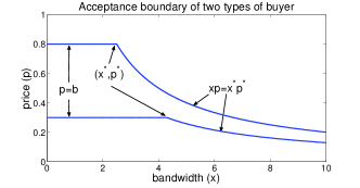
For a given buyer type ($q,\epsilon,b$), the seller can choose any point in the corresponding acceptance region $T$ to maximize its utility: $\max_{(x,p)\in T}U(x,p)$. We next show that the optimal contract for the seller is given by the “knee” (the intersection point where the straight line meets the curve) on the boundary of the acceptance region, denoted as $(x^{*},p^{*})$.

Theorem 2.

The optimal contract for the seller is the intersection point $(x^{*},p^{*})$ on the acceptance region boundary of the buyer.

Proof.

We prove the optimality in two steps. First we show that the seller’s utility is strictly increasing in $p$ which implies that the optimal contract must be such that (5) and (8) hold with strict equality. Then we show that the intersection point is strictly better than any other point on the boundary. For any $x>0$ and $\forall p^{\prime}>p$, we have

$$U(x,p^{\prime})=x(p^{\prime}-c)>x(p-c)=U(x,p).$$

Thus $U(x,p)$ is strictly increasing in $p$. For any $x<x^{*}$ (points on the straight line) we have

$$U(x^{*},p^{*})=x^{*}(p^{*}-c)>x(p^{*}-c)=U(x,p^{*}),$$

which used the fact that $p^{*}>c$. (Recall we have assumed that for any buyer there must exist a contract with $p>c$ that it finds acceptable. This implies such a point must be within the acceptance region, which in turn implies that we must have $p^{*}>c$ since $p^{*}\geq p$, $\forall p$ in the region.) For any pair $(x,p)$ such that $xp=x^{*}p^{*}$ and $x>x^{*}$ (points on the curve),

$$U(x,p)=x(p-c)=x^{*}p^{*}-xc>x^{*}(p^{*}-c)=U(x^{*},p^{*}).$$

Thus $U(x^{*},p^{*})$ is strictly greater than any point $U(x,p)$ on the boundary. ∎

Once the seller determines the optimal contract and presents it to the buyer, the buyer will accept because it satisfies both the loss and the IR constraints. It can be easily shown that the buyer’s cost in accepting is exactly $C(0,0)$. Note that technically since the cost of the contract is exactly equal to the reserve price, the buyer is ambivalent between getting only deterministic service and getting a mix of both types of services. In practice the seller can always lower the unit price $p^{*}$ by an arbitrarily small amount to provide a positive incentive so that the buyer will accept the contract. For this reason even though the costs are equal, for simplicity we will assume that the buyer will accept this contract. For the same reason, we will also assume that when there exist multiple contracts of equal cost to the buyer, the seller can always induce the desired choice from the buyer by introducing a small difference to the desired contract. We have now a complete characterization of the contract design for a single type of buyer. We end this section by introducing the concept of an equal-cost line of a buyer. Consider a contract $(x^{\prime},p^{\prime})$. Denote by $P(x^{\prime},p^{\prime},x)$ a price such that the contract $(x,P(x^{\prime},p^{\prime}$ $,x))$ has the same cost as contract $(x^{\prime},p^{\prime})$ to a buyer.

Definition 1.

The equal-cost line $E$ of a buyer of type $(q,\epsilon,b)$ is the set of contracts within the buyer’s acceptance region $T$ that are of equal cost to the buyer. Thus $(x,p)\in E$ if and only if $p=P(x^{\prime},p^{\prime},x)$ for some other $(x^{\prime},p^{\prime})\in E$. The cost of this line is given by $C(x^{\prime},p^{\prime})$, $\forall(x^{\prime},p^{\prime})\in E$.

It should be clear that there are many equal-cost lines, each with a different cost. Figure 2 shows an example of a set of equal-cost lines. We will therefore also write an equal-cost line as $E_{x^{\prime},p^{\prime}}$ for some $(x^{\prime},p^{\prime})$ on the line to distinguish it from other equal-cost lines. The next theorem gives a precise expression for the equivalent price that characterizes an equal-cost line.

Figure 2: Example of equal cost lines

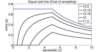
Theorem 3.

For a buyer of type $(q,\epsilon,b)$ with an intersection point $(x^{*},p^{*})$ on its acceptance region boundary, and given a contract $(x^{\prime},p^{\prime})$, an equal-cost line $E_{x^{\prime},p^{\prime}}$ consists of all contracts $(x,P(x^{\prime},p^{\prime},x))$ such that

$$P(x^{\prime},p^{\prime},x)=\left\{\begin{tabular}[]{ll}$b-\frac{x^{\prime}}{x}(b-p^{\prime})$&if $x,x^{\prime}\leq x^{*}$\\ $x^{\prime}p^{\prime}/x$&if $x,x^{\prime}\geq x^{*}$\\ $(b(x^{*}-x^{\prime})+x^{\prime}p^{\prime})/x$&if $x^{\prime}<x^{*}<x$\\ $b-(x^{*}b-x^{\prime}p^{\prime})/x$&if $x<x^{*}<x^{\prime}$\end{tabular}\right.$$

Proof.

We will prove this for the case $q(1-b)\leq\epsilon$; the other case can be shown with similar arguments and is thus omitted for brevity. In this case $x^{*}=\frac{q-\epsilon}{b}$. When $x,x^{\prime}\leq x^{*}$, without buying deterministic service the loss is given by

$$E[(q-xB)^{+}] = (q-x)^{+}b+q(1-b)$$

$$= (q-x)b+q(1-b)=q-xb\geq\epsilon,$$

where the second equality is due to the fact that $q(1-b)\leq\epsilon\Rightarrow\frac{q-\epsilon}{b}\leq q\Rightarrow x\leq\frac{q-\epsilon}{b}\leq q$. The incentive for the buyer is to purchase $y$ such that the loss is just equal to $\epsilon$.

$$E[(q-y-xB)^{+}] = (q-y-x)b+(q-y)(1-b)$$

$$= q-y-xb=\epsilon~{}.$$

The first equality follows from the fact that $q(1-b)\leq\epsilon$, which implies both $(q-y-x)\geq 0$ and $(q-y)\geq 0$. This is true for both $(x,p)$ and $(x^{\prime},p^{\prime})$. Since $(x,p)$ is on the equal cost line $E_{x^{\prime},p^{\prime}}$, we know that $C(x,p)=C(x^{\prime},p^{\prime})$. We also know that $C(x,p)=y+xp$ and $C(x^{\prime},p^{\prime})=y^{\prime}+x^{\prime}p^{\prime}$,

$$C(x,p)=q-\epsilon-xb+xp=q-\epsilon-x^{\prime}b+x^{\prime}p^{\prime}=C(x^{\prime},p^{\prime})~{}.$$

Rearranging the second equality such that $p$ is a function of $x,x^{\prime},p^{\prime}$ immediately gives the result. When $x,x^{\prime}>x^{*}$, $x$ ($x^{\prime}$) alone is sufficient to achieve the loss constraint. For $C(x,p)=C(x^{\prime},p^{\prime})$ we must have $x^{\prime}p^{\prime}=xp$, resulting in the second branch. The third and fourth branch can be directly derived from the first two branches. When $x>x^{*}>x^{\prime}$ ($x^{\prime}>x^{*}<x$), we first find the equivalent price at $x^{*}$ by the first branch (second branch), and then use the second branch (first branch) to find $P(x^{\prime},p^{\prime},x)$. This gives the third branch (fourth branch)∎∎

The form of the equal-cost line is the same regardless whether $q(1-b)\leq\epsilon$ or $q(1-b)>\epsilon$. Note that every contract below an equal-cost line is strictly preferable to a contract on the line for the buyer. This is an observation we will use in subsequent sections. We end this section with a property of the equivalent price we will use later.

Lemma 2.

$P(x^{\prime},p^{\prime},x)$ is strictly increasing in $p^{\prime}$ when $x^{\prime}>0$.

This lemma is easily shown by noting $C(x^{\prime},p^{\prime})=y+x^{\prime}p^{\prime}$, where $y$ is only a function of $x^{\prime}$. Thus, $p>p^{\prime}$ implies $C(x^{\prime},p)>C(x^{\prime},p^{\prime})$ when $x^{\prime}>0$.

IV Common channel condition

We now consider $K$ types of buyers indexed by $i=1,2,\cdots,K$, each defined by the triple $(q_{i},\epsilon_{i},b_{i})$ with an associated acceptance region $T_{i}$. We will use the notation

$$max_{i}=(x_{i}^{*},p_{i}^{*})=\mbox{argmax}_{(x,p)\in T_{i}}U(x,p)$$

to denote the optimal contract if type $i$ were the only type existing. Similarly, we will use $C_{i}(x,p)$ to denote the cost to a type-$i$ buyer for accepting contract $(x,p)$.

A buyer is of type $i$ with probability $r_{i}$. We assume that the seller knows only this distribution of types but not the actual type of a given buyer. Consequently it has to design the contracts in a way that maximizes its expected payoff. Since the payoff is measured in expectation, it turns out that it does not matter whether the seller is faced with a single buyer or multiple buyers as long as they are drawn from the same, known type distribution and the seller has sufficient bandwidth to honor its contracts. For this reason throughout our discussion we will take the view of a single buyer drawn from a certain type distribution. In Section VI we discuss the case when the seller has limited bandwidth to trade.

Consider a set of contracts $\mathbb{C}=\{(x_{1},p_{1}),...,(x_{K},p_{K})\}$ designed by the seller with the intention that a buyer of type $i$ prefers $(x_{i},p_{i})$. This is true iff

$$C_{i}(x_{i},p_{i})\leq C_{i}(x_{j},p_{j}) \forall j\neq i~{}.$$

Let $R_{i}(\mathbb{C})$ denote the contract that a type-$i$ buyer selects given a set $\mathbb{C}$. Then $R_{i}(\mathbb{C})=\text{argmin}_{(x,p)\in\mathbb{C}}~{}C_{i}(x,p)$ and the seller’s expected utility for a given $\mathbb{C}$ is $E[U(\mathbb{C})]=\sum_{i}U(R_{i}(\mathbb{C}))r_{i}$

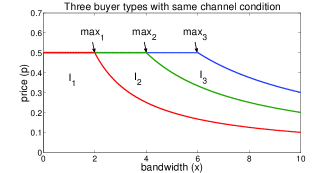
In this section we consider the case where different types share the same channel condition $b_{i}=b,i=1,\cdots,K$, which is also known to the seller. As mentioned earlier, this models the case where the condition is primarily determined by the seller’s primary user traffic. An example of the acceptance regions of three buyer types are shown in Figure 3; note that $max_{i}$’s need not be ordered in $i$. There are two possible cases: (1) the seller can announce as many contracts as he likes ($M=K$; note that there is no point in designing more contracts than the number of types); (2) the seller is limited to at most $M<K$ contracts. Below we fully characterize the optimal contract set in both cases.

Figure 3: Three buyer types with common $b$

Theorem 4.

When $M=K$, the contract set that maximizes the seller’s profit is $(max_{1},max_{2},...,max_{K})$.

This result holds for the following reason. As shown in Figure 3, with a constant $b$, the intersection points of all acceptance regions are on the same line $p=b$. For a buyer of type $i$, all points to the left of $max_{i}$ on this line cost the same as $max_{i}$, and all points to its right are outside the buyer’s acceptance region. Therefore the type-$i$ buyer will select the contract $max_{i}$ given this contract set (see earlier discussion on how the seller can always incentivize this contract over others with equal cost). Since this is the best the seller can do with a type-$i$ buyer (see Theorem 3) this set is optimal for the seller. It is also relatively straightforward to obtain a similar results in the case of $M<K$ given next.

Lemma 3.

When $M<K$ and $\forall b_{i}=b$, the optimal contract set is a subset of $(max_{1},...,max_{K})$.

Proof.

Assume the optimal contract $\mathbb{C}$ is not a subset of $(max_{1},...,max_{K})$. Then it must consists of some contract points from at least one of the $I_{i}$ regions as demonstrated in Figure 3. Let these contracts be $A_{i}\subset I_{i}$ and $\bigcup_{i}A_{i}=\mathbb{C}$. For each non-empty $A_{i}$, we replace it by the contract $max_{i}$ and call this new contract set $\mathbb{C^{\prime}}$. The proof is to show that this contract set generates profit at least as large as the original one. For each type-$i$ buyer that picked some contract $(x,p)\in A_{j}$ from the optimal contract $\mathbb{C}$, it must had a type greater than or equal to $j$ otherwise $(x,p)$ is not in its acceptance region. In the contract set $\mathbb{C^{\prime}}$, type-$i$ will now pick $max_{j}$ or $max_{l}$ with $l>j$. The choice of each possible type of buyer picks from $\mathbb{C^{\prime}}$ is at least as profitable as the one they picked from $\mathbb{C}$. Thus, the expected profit of $\mathbb{C^{\prime}}$ is at least as good as $\mathbb{C}$. ∎

This lemma suggests the following iterative way of finding the optimal contract set without having to solve what would seem like a combinatorial problem. Define function $g(m,i)$ as the the maximum expected profit for the seller by picking contract $max_{i}$ and selecting optimally $m-1$ contracts from the set $(max_{i+1},...,max_{K})$. Note that if we include $max_{i}$ and $max_{j}$ ($i<j$) in the contract set but nothing else in between $i$ and $j$, then a buyer of type $l$ ($i\leq l<j$) will pick contract $max_{i}$. These types contribute to an expected profit of $x_{i}^{*}(b-c)\sum_{l=i}^{j-1}r_{l}$. At the same time, no types below $i$ will select $max_{i}$ (as it is outside their acceptance regions), and no types at or above $j$ will select $max_{i}$ (as for them $max_{j}$ is preferable).

The function $g(m,i)$ can be recursively obtained as follows:

$$g(m,i)=\underset{j:i<j\leq K-m+2}{max}g(m-1,j)+x_{i}^{*}(b-c)\sum_{l=i}^{j-1}r_{l},$$

with the boundary condition $g(1,i)=x_{i}^{*}(b-c)\sum_{l=i}^{K}r_{l}$.

Finally, it should be clear that the maximum expected profit for the seller is given by $\max_{1\leq i\leq K}g(M,i)$, and the optimal contract set can be determined by going backwards: first determine $i^{*}_{M}=\arg\max_{1\leq i\leq K}g(M,i)$, then $i^{*}_{M-1}=\arg\max_{1\leq i\leq K-1}g(M-1,i)$, and so on.

Theorem 5.

The set $\{max_{i^{*}_{1}},max_{i^{*}_{2}},\cdots,max_{i^{*}_{M}}\}$ obtained using the above procedure is optimal and its expected profit is given by $g(M,i^{*}_{M})$.

V Private channel condition

We now consider multiple buyer types each with a different channel condition $b_{i}$, $i=1,\cdots,K$. We will start with the special case of $K=2$ and characterize the optimal contracts in this case. Using these results we then construct an algorithm to compute a set of contracts for the case of $K\geq 2$.

V-A Two buyer types: $K=2$

Consider two buyer types $(q_{i},\epsilon_{i},b_{i})$, $i=1,2$, with probability $r_{i}$, $r_{1}+r_{2}=1$. We first consider the case that the seller is limited to one contract: $M=1$.

Figure 4: (left) $max_{1}\notin T_{2}$ and $max_{2}\notin T_{1}$; (right) $max_{1}\in T_{2}$

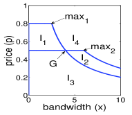
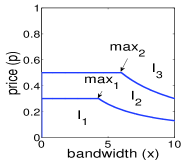
Theorem 6.

The optimal contract when $K=2$ and $M=1$ is as follows:

1. If $max_{1}\notin T_{2}$ and $max_{2}\notin T_{1}$,

   $$\mbox{optimal}=\left\{\begin{tabular}[]{cl}$max_{1}$&\mbox{if} ~{} $r_{1}U(max_{1})\geq r_{2}U(max_{2})$\\ &~{}~{}~{} \mbox{and} ~{} $r_{1}U(max_{1})\geq U(G)$\\ $max_{2}$&if ~{} $r_{2}U(max_{2})\geq r_{1}U(max_{1})$\\ &~{}~{}~{} \mbox{and} ~{} $r_{2}U(max_{2})\geq U(G)$\\ $G$&if ~{} $U(G)\geq r_{2}U(max_{2})$\\ &~{}~{}~{} \mbox{and} ~{} $U(G)\geq r_{1}U(max_{1})$\\ \end{tabular}\right.$$

   where $G$ denotes the intersecting point between acceptance region boundaries of the two types.

2. If $max_{1}\in T_{2}$.

   $$optimal=\left\{\begin{tabular}[]{cc}$max_{1}$&if ~{} $U(max_{1})\geq r_{2}U(max_{2})$\\ $max_{2}$&if ~{} $r_{2}U(max_{2})\geq U(max_{1})$\\ \end{tabular}\right.$$

3. If $max_{2}\in T_{1}$.

   $$optimal=\left\{\begin{tabular}[]{cc}$max_{2}$&if $U(max_{2})\geq r_{1}U(max_{1})$\\ $max_{1}$&if $r_{1}U(max_{1})\geq U(max_{2})$\\ \end{tabular}\right.$$

The above result is illustrated in Figure 4 and can be argued by showing the profit of every contract in a particular region (such as $I_{1}$) is no greater than some specific contract (such as $max_{1}$). Take the case $max_{1}\notin T_{2}$ and $max_{2}\notin T_{1}$ for example, any point in $I_{3}$ is suboptimal to point $G$ because any contract in $I_{3}$ is acceptable by both types of buyers, but $G$ has a strictly higher profit than any other point in $I_{3}$.

We now consider the case $M=2$. We shall see that providing multiple contracts can help the obtain higher profits.

Theorem 7.

In the case of $M=2$, $max_{1}\notin T_{2}$ and $max_{2}\notin T_{1}$, the optimal contract set is $\{max_{1},max_{2}\}$.

Proof.

The set $\mathbb{C}=\{max_{1},max_{2}\}$ gives an expected payoff of

$$E[U(\mathbb{C})] = r_{1}U(R_{1}(\mathbb{C}))+r_{2}U(R_{2}(\mathbb{C})))$$

$$= r_{1}U(R_{1}(max_{1}))+r_{2}U(R_{2}(max_{2})).$$

The second equality holds because $max_{1}\notin T_{2}$ and $max_{2}$ $\notin T_{1}$ and thus type $i$ will pick $max_{i}$. Suppose $\mathbb{C}$ is not the optimal set of 2 contracts, then there must exists some $\mathbb{C^{\prime}}=\{(x_{1},p_{1}),(x_{2},p_{2})\}$ such that

$$E[U((\mathbb{C^{\prime}}))] = r_{1}U(R_{1}(x_{1},p_{1}))+r_{2}U(R_{2}(x_{2},p_{2}))$$

$$> E[U(\mathbb{C})]$$

$$= r_{1}U(R_{1}(max_{1}))+r_{2}U(R_{2}(max_{2}))$$

This implies either $U(R_{1}(x_{1},p_{1}))>U(R_{1}(max_{1}))$, or $U(R_{2}(x_{2},p_{2}))>U(R_{2}(max_{2}))$, or both, all of which contradict the definition of $max_{i}$. Thus, $\{max_{1},max_{2}\}$ is the optimal contract set. ∎

The proof as well as the intuition behind the above result are straightforward. The next case, $M=2$, $max_{1}\in T_{2}$ or $max_{2}\in T_{1}$, is more complicated. Without loss of generality, we will assume that the type-$1$ buyer has a smaller $b_{1}$ ($b_{1}\leq b_{2}$), thus $max_{1}\in T_{2}$. We first determine the optimal contract when $x^{*}_{1}\leq x^{*}_{2}$; this result is then used for the case when $x_{1}^{*}>x_{2}^{*}$. Without loss of optimality we consider only contract pairs $\{(x_{1},p_{1}),(x_{2},p_{2})\}$ where type-$i$ buyer picks $(x_{i},p_{i})$ instead of the other one.

To find the optimal contract, we 1) first show that for each $(x_{1},p_{1})$ we can express the optimal $(x_{2},p_{2})$ in terms of $x_{1}$ and $p_{1}$; 2) then we show that $(x_{1},p_{1})$ must be on the boundary of $T_{1}$ with $x_{1}\leq x_{1}^{*}$; 3) using 1) and 2) we optimize the expected profit over possible choices of $x_{1}$.

Lemma 4.

When $K=2$, if $max_{1}\in T_{2}$ and $x_{1}^{*}\leq x_{2}^{*}$, then given a contract for type-1 $(x_{1},p_{1})$, the optimal contract for type-$2$ must be $(x_{2}^{*},P_{2}(x_{1},p_{1},x_{2}^{*}))$.

Proof.

Given a contract $(x_{1},p_{1})$, the feasible region for the contract of type-$2$ buyer is the area below $P_{2}(x_{1},p_{1},x)$ as defined in Theorem 3 (see Figure 5). Since the seller’s profit is increasing in both $p$ and $x$, the contract that generates the highest profit is at $x_{2}=x_{2}^{*}$ and $p_{2}=P_{2}(x_{1},p_{1},x_{2}^{*})$. ∎

Lemma 5.

When $K=2$, if $max_{1}\in T_{2}$ and $x_{1}^{*}\leq x_{2}^{*}$, an optimal contract for type-1 must be $p_{1}=b_{1}$ and $x_{1}\leq x_{1}^{*}$.

This lemma suggests that the optimal contract for type-1 lies on the straight line portion of its boundary; this can be shown using proof by contradiction. Using Lemmas 4, 5 and Theorem 3, the expected profit can be expressed as follows.

Proof.

Lemma 5 can be proved in two steps. First we assume the optimal contract has $(x_{1},p_{1})\in T_{1}$, where we can increase $p_{1}$ by some positive $\delta>0$ but still have $(x_{1},p_{1}+\delta)\in T_{1}$. By noticing that both $U(x,p)$ and $P(x,p,x^{\prime})$ are increasing in $p$. We know that both $U(x_{1},p_{1}+\delta)$ and $U(x_{2}^{*},P_{2}(x_{1},p_{1}+\delta,x_{2}^{*})))$ are strictly larger than $U(x_{1},p_{1})$ and $U(x_{2}^{*},P_{2}(x_{1},p_{1},x_{2}^{*})))$. This contradicts the assumption that it was optimal before, thus, we know that the optimal contract for $(x_{1},p_{1})$ must be on the two lines (the upper boundary of $T_{1}$) defined in Theorem 1. Then we can exclude the possibility of having $(x_{1},p_{1})$ on the boundary of $T_{1}$ with $x_{1}>x_{1}^{*}$ by comparing the contract $(x_{1}^{*},b_{1})$ with such a contract. ∎

Figure 5: The regions to distinguish type-2 given $(x_{1},p_{1})$

$$E[U(\mathbb{C})] = r_{1}U(x_{1},p_{1})+r_{2}U(x_{2},P_{2}(x_{1},p_{1},x_{2}^{*}))$$

$$= r_{1}U(x_{1},b_{1})+r_{2}U(x_{2}^{*},b_{2}-\frac{x_{1}}{x_{2}^{*}}(b_{2}-b_{1}))$$

$$= r_{1}x_{1}(b_{1}-c)+r_{2}x_{2}^{*}(b_{2}-\frac{x_{1}}{x_{2}^{*}}(b_{2}-b_{1})-c)$$

$$\frac{\partial E[U(\mathbb{C})]}{\partial x_{1}} = r_{1}(b_{1}-c)-r_{2}(b_{2}-b_{1})$$

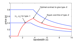
The $x_{1}$ acheiving the optimal contract $\mathbb{C}$ is given by,

$$x_{1} =\begin{cases}0&\text{if~{}}r_{1}(b_{1}-c)-r_{2}(b_{2}-b_{1})<0\\ x_{1}^{*}&\text{if~{}}r_{1}(b_{1}-c)-r_{2}(b_{2}-b_{1})>0\end{cases}$$

$$\mathbb{C} =\begin{cases}\{max_{2}\}~{}~{}~{}~{}~{}~{}~{}~{}\text{if~{}}r_{1}(b_{1}-c)-r_{2}(b_{2}-b_{1})<0\\ \{max_{1},(x_{2}^{*},b_{2}-\frac{x_{1}^{*}}{x_{2}^{*}}(b_{2}-b_{1}))\}~{}~{}~{}~{}~{}~{}~{}~{}~{}~{}~{}~{}~{}\text{o.w.}\end{cases}$$

This result shows two operating regimes: 1) When $\frac{r_{1}}{r_{2}}<\frac{b_{2}-b_{1}}{b_{1}-c}$, type-$2$ is more profitable and the seller will distribute $max_{2}$. In this case there is no way to distribute another contract for type-$1$ without affecting the behavior of type-$2$. Consequently, the seller only distributes one contract. 2) When $\frac{r_{1}}{r_{2}}>\frac{b_{2}-b_{1}}{b_{1}-c}$, type-$1$ is more profitable and the seller will distribute $max_{1}$. After choosing $max_{1}$, the seller can also choose $(x_{2}^{*},b_{2}-\frac{x_{1}^{*}}{x_{2}^{*}}(b_{2}-b_{1}))$ for the type-$2$ buyer without affecting the type-$1$ buyer’s choice. As a result, the seller distributes a pair of contracts to get the most profit. The optimal contract for $x_{1}^{*}>x_{2}^{*}$ can be determined with a similar argument.

Again, we can prove that the optimal contract must have $p_{1}=b_{1}$ and $x_{1}\leq x_{1}^{*}$. The difference is that when $x_{1}^{*}>x_{2}^{*}$, the expression for $(x_{2}^{*},P_{2}(x_{1},p_{1},x_{2}^{*}))$ has two cases depending on whether $x_{1}>x_{2}^{*}$ or $x_{1}\leq x_{2}^{*}$.

$$E[U(\mathbb{C})]=$$

$$~{}~{}\begin{cases}r_{1}U(x_{1},b_{1})+r_{2}U(x_{2}^{*},b_{2}-\frac{x_{1}}{x_{2}^{*}}(b_{2}-b_{1}))&\text{if~{}}x_{1}\leq x_{2}^{*}\\ r_{1}U(x_{1},b_{1})+r_{2}U(x_{2}^{*},\frac{x_{1}b_{1}}{x_{2}^{*}})&\text{if~{}}x_{1}>x_{2}^{*}\end{cases}$$

$$\frac{\partial E[U(\mathbb{C})]}{\partial x_{1}}=\begin{cases}r_{1}(b_{1}-c)-r_{2}(b_{2}-b_{1})&\text{if~{}}x_{1}\leq x_{2}^{*}\\ r_{1}(b_{1}-c)+r_{2}b_{1}&\text{if~{}}x_{1}>x_{2}^{*}\end{cases}$$

To summarize, when $r_{1}(b_{1}-c)-r_{2}(b_{2}-b_{1})>0$, $E[R(\mathbb{C})]$ is strictly increasing in $x_{1}$ and we know that $x_{1}=x_{1}^{*}$ maximizes the expected profit. When $r_{1}(b_{1}-c)-r_{2}(b_{2}-b_{1})<0$, $E[R(\mathbb{C})]$ is decreasing in $x_{1}$ if $x_{1}\in[0,x_{2}^{*}]$ and increasing in $x_{1}$ if $x_{1}\in[x_{2}^{*},x_{1}^{*}]$. We can only conclude that either $x_{1}=0$ or $x_{1}=x_{1}^{*}$ maximizes the expected profit.

$$x_{1}=\begin{cases}0\text{~{}or~{}}x_{1}^{*}&\text{if~{}}r_{1}(b_{1}-c)-r_{2}(b_{2}-b_{1})<0\\ x_{1}^{*}&\text{if~{}}r_{1}(b_{1}-c)-r_{2}(b_{2}-b_{1})>0\end{cases}$$

$$\mathbb{C}=$$

$$\begin{cases}max_{2}\text{/}\{max_{1},(x_{2}^{*},\frac{x_{1}^{*}b_{1}}{x_{2}^{*}})\}&\text{if~{}}r_{1}(b_{1}-c)-r_{2}(b_{2}-b_{1})<0\\ \{max_{1},(x_{2}^{*},\frac{x_{1}^{*}b_{1}}{x_{2}^{*}})\}&\text{if~{}}r_{1}(b_{1}-c)-r_{2}(b_{2}-b_{1})>0\end{cases}$$

In the first condition, we can calculate the expected profit of the two contract sets and pick the one with the higher profit.

V-B $K$ buyer types, $K>2$

The previous section gives the explicit solution to the contract design problem when $K=2$. When $K>2$ we no longer have explicit solutions; even numerically searching for the optimal contract set becomes very complicated. For instance, even if we assume that both $x$ and $p$ are from discrete sets, with $X$ and $P$ possible values, respectively, the search must be done over the space of all possible sets of $K$ different contracts, on the order of $(XP)^{K}$. In general $X$ and $P$ both take on real values, making the search space uncountable. In order to reduce the complexity we will need to exploit special properties of the problem. We first reindex the buyer types such that $b_{1}\leq...\leq b_{K}$, under certain conditions we will determine a procedure which finds the optimal contract.

Definition 2.

The buyer types are said to satisfy a monotonicity condition (MC), if $\forall i,j$, $b_{i}\leq b_{j}$ implies $x_{i}^{*}\leq x_{j}^{*}$. (Remember we will reindexed the types so that $b_{1}\leq...\leq b_{K}$ and thus $x_{1}^{*}\leq...\leq x_{K}^{*}$)

This monotonicity condition (MC) says that the amount a buyer willing to buy is strictly increasing in the quality it gets from buying the secondary spectrum. This condition leads to special properties which allows us to construct simpler ways to find the optimal contracts.

Theorem 8.

When the MC is satisfied, $b_{i}\leq b_{j}$ and $x<x^{\prime}$ implies $P_{i}(x^{\prime},p^{\prime},x)\geq P_{j}(x^{\prime},p^{\prime},x)$.

Theorem 9.

When the MC is satisfied, $b_{i}\leq b_{j}$ and $x>x^{\prime}$ implies $P_{i}(x^{\prime},p^{\prime},x)\leq P_{j}(x^{\prime},p^{\prime},x)$.

Proof.

The proofs for Theorem 8 and Theorem 9 are moved to the Appendix. ∎

Lemma 6.

When the MC is satisfied, the optimal contract such that type i buyer picks $(x_{i},p_{i})$ for all i must have $x_{1}\leq...\leq x_{K}$.

Proof.

Let $(x_{i},p_{i})$ denote the contract designed for the type i buyer. Consider now the contract for the type j buyer where $b_{j}<b_{i}$ and $x_{j}>x_{i}$. From Theorem 9 we know that $P_{j}(x_{i},p_{i},x_{j})\leq P_{i}(x_{i},p_{i},x_{j})$ when the MC is satisfied. This implies that whatever $p_{j}$ we determined, if the type j buyer prefers $(x_{j},p_{j})$ over $(x_{i},p_{i})$ then the type i buyer must think the same way. From the IC constraint, the type j buyer has to prefer the $(x_{j},p_{j})$ over $(x_{i},p_{i})$. Thus, we must have $x_{j}\leq x_{i}$ in the optimal contract where each type of buyer selects its own designated contract. ∎

Figure 6: Example of a possible optimal contract

Lemma 7.

When the MC is satisfied, the optimal contract must have $x_{i}\leq x_{i}^{*}$ $\forall i=1...K$.

Proof.

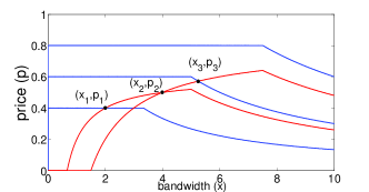
Proof by contradiction. Consider some optimal contract having $x_{i}>x_{i}^{*}$, we show that replacing $x_{i}=x_{i}^{*}$ is actually better. By Theorem 10, we know that $p_{i}=P_{i}(x_{i-1},p_{i-1},x_{i})$ and by definition of $P_{i}$ it is better off to the seller by providing $x_{i}^{*}$ instead if we only consider the profit from the type $i$ buyer. Now, by Theorem 8 $P_{i+1}(x_{i},p_{i},x_{i}^{*})\leq P_{i}(x_{i},p_{i},x_{i}^{*})$. Also, because $P_{i}(x^{\prime},p^{\prime},x)$ is a strictly increasing function in $p^{\prime}$. The price $p_{i+1}$ is strictly higher for assigning $x_{i}^{*}$ instead of $x_{i}$. This results in every $p_{j}$ $j>i$ is strictly increased and the payoff change must be positive. The only question is whether we can assign $x_{i}^{*}$ without affecting the contracts $(x_{j},p_{j})$ $j<i$. The answer is if $\forall j<i$ $x_{j}\leq x_{j}^{*}$ we can do it. By mathematical induction, we can again prove that for all $i=1...K$ $x_{i}\leq x_{i}^{*}$. An example is illustrated in Figure 6. ∎

This result allows us to restrict our search for the optimal contract to the set where $x_{i}\leq x_{i}^{*}$. We can further simplify our search by expressing the values $p_{i}$, $\forall i=1...K$ as functions of $x_{i}$ $\forall i=1...K$, by the following theorem.

Theorem 10.

Given a set $x_{1}\leq...\leq x_{K}$, define $(x_{0},p_{0})=(0,0)$ and find the contracts $(x_{i},p_{i})=(x_{i},P_{i}(x_{i-1},p_{i-1},x_{i}))$ in the order $i=1...K$. When the MC is satisfied this procedure produces a contract set that maximizes the seller’s profit, where each type-$i$ buyer accepts $(x_{i},p_{i})$.

Proof.

1. Each buyer of type $i$ picks $(x_{i},p_{i})$.
   Induction hypothesis: At each step, when we pick contract $(x_{i},p_{i})$ $\forall i=0...K$, each buyer type-$j$ with $j<i$ prefers contract $(x_{j},p_{j})$ and each buyer type-$j$ with $j\geq i$ prefers contract $(x_{i},p_{i})$.

   1. Base Case: When picking $(x_{0},p_{0})=(0,0)$, it is clear that each buyer type is greater than $0$ and each buyer prefers the only contract that is the same as (as good as) not buying.

   2. Assume the induction hypothesis is true when picking $(x_{i},p_{i})$, we will show that the hypothesis is also true for $(x_{i+1},p_{i+1})$. Assume the hypothesis is true for step $i$ means we have determined the contracts $((x_{1},p_{1}),...,(x_{i},p_{i}))$ and a type-$j$ buyer ($j\leq i$) prefers $(x_{j},p_{j})$ over other contracts, while a type-$j$ buyer ($j>i$) prefers the $i$th contract over all contracts.

      $$p_{i+1}=(x_{i+1},P_{i+1}(x_{i},p_{i},x_{i+1}))$$

      By Theorem. 9 and $x_{i+1}>x_{i}$, $\forall j\leq i$

      $$p_{i+1}=P_{i+1}(x_{i},p_{i},x_{i+1})\geq P_{j}(x_{i},p_{i},x_{i+1})$$

      The contract $(x_{i+1},p_{i+1})$ is above the equal cost line of the contract $(x_{i},p_{i})$ for buyer type less than or equal to $i$. Which means they prefer the $i$th contract over the $i+1$th contract. But from step $i$, they prefer their own contract over existing contracts. Thus, buyer $j$ $(j\leq i)$ prefers $(x_{j},p_{j})$ over all contracts. By Theorem. 8 and $x_{i+1}>x_{i}$, $\forall j\geq i+1$

      $$p_{i+1}=P_{i+1}(x_{i},p_{i},x_{i+1})\leq P_{j}(x_{i},p_{i},x_{i+1})$$

      Thus, the contract $(x_{i+1},p_{i+1})$ is below the equal cost line of the contract $(x_{i},p_{i})$ for buyer type $j>i$. Which means they prefer $(x_{i+1},p_{i+1})$ over $(x_{i},p_{i})$. But from step $i$, they prefer the $(x_{i},p_{i})$ contract over all existing contracts. This shows that the hypothesis is true for step $i+1$.

   3. By Mathematical Induction, the hypothesis is true for all $i\leq K$.

2. This process results in the highest profit.
   Since the $x_{i}^{\prime}s$ are fixed, the only way one could increase the buyer’s profit is to increase one of the $p_{i}$’s. We will show that this is not possible. Assume there exists some contract with the contract set $(x_{1},p_{1}^{\prime})...(x_{K},p_{K}^{\prime})$ with some $p_{i}^{\prime}>p_{i}$, by the increasing property of $P_{i}$ (Lemma 2) we need $p_{i-1}^{\prime}>p_{i-1}$ to insure that type-$i$ buyer picks $(x_{i},p_{i}^{\prime})$. By induction, we can show that it must be that $(p_{1}^{\prime}>p_{1})$. Since $p_{1}=P_{1}(0,0,x_{1})=b_{1}$, $(x_{1},p_{1})$ is already on the boundary of acceptance region of the type-$1$ buyer. Thus, any contract with some $p_{i}^{\prime}>p_{i}$ is not a contract where each buyer accepts its own designated contract.

∎

Figure 6 shows an example of applying this theorem with three buyer types: given $x_{1}=2$, $x_{2}=4$, $x_{3}=6$, $p_{i}$ is sequentially determined on the equal-cost line of the previous contract. With Lemma 7, the equal cost line can be restricted to the form $P_{i}(x_{i-1},p_{i-1},x_{i})=b_{i}-\frac{x_{i-1}}{x_{i}}(b_{i}-p_{i-1})$. The expected profit of the seller can now be expressed as:

$$E[R(\mathbb{C})]=\underset{x_{1},..,x_{K}}{max}r_{1}x_{1}(b_{1}-c)$$

$$~{}~{}~{}~{}~{}~{}~{}~{}~{}~{}~{}~{}~{}~{}~{}~{}~{}+...+r_{i}x_{i}(p_{i}-c)+...+r_{K}x_{K}(p_{K}-c)$$

$$=\underset{x_{1}\leq...\leq x_{K}}{max}r_{1}x_{1}(b_{1}-c)+...+r_{i}x_{i}(P_{i}(x_{i-1},p_{i-1},x_{i})-c)$$

$$~{}~{}~{}~{}~{}~{}~{}~{}~{}~{}~{}~{}~{}~{}~{}~{}~{}+...+r_{K}x_{K}(P_{K}(x_{K-1},p_{K-1},x_{K})-c)$$

By plugging in the values of $p_{i}=P_{i}(x_{i-1},p_{i-1},x_{i})=b_{i}-\frac{x_{i-1}}{x_{i}}(b_{i}-p_{i-1})$ recursively. Each term in the optimization problem can be simplified to

$$r_{i}x_{i}(p_{i}-c)=r_{i}(x_{i}(b_{i}-c)-\sum_{j=1}^{i-1}x_{j}(b_{j+1}-b_{j}))$$

By simplifying and separate the terms with respect to $x_{i}$, the expected profit of the seller can be expressed as,

$$E[R(\mathbb{C})]=\underset{x_{1}\leq...\leq x_{K}}{max}\sum_{i=1}^{K}x_{i}\left(r_{i}(b_{i}-c)-(b_{i+1}-b_{i})\sum_{j=i+1}^{K}r_{j}\right)$$

Firstly, we observe that the above expression is linear in every $x_{i}$. Thus differentiating with respect to $x_{i}$ we get a constant:

$$\frac{\partial E[R(\mathbb{C})]}{\partial x_{i}}=r_{i}(b_{i}-c)-\sum_{j=i+1}^{K}r_{j}(b_{i+1}-b_{i})$$

Secondly, because the term $\frac{\partial E[R(\mathbb{C})]}{\partial x_{i}}$ does not depend on any $x_{j}$, the optimizer can be easily determined. When $\frac{\partial E[R(\mathbb{C})]}{\partial x_{i}}>0$ we want to make $x_{i}$ as large as possible ($\leq x_{i}^{*}$); when $\frac{\partial E[R(\mathbb{C})]}{\partial x_{i}}<0$ we want to make $x_{i}$ as small as possible. This leads us to the following algorithm which finds the optimal set of $(x_{1},...,x_{K})$. The variable $LD$ (Last Determined) below is used to keep track of the last type for which we have already determined its value.

Step 1

. Since $\frac{\partial E[R(\mathbb{C})]}{\partial x_{K}}=r_{K}(b_{K}-c)>0$, let $x_{K}=x_{K}^{*}$.
Set $LD=K$, $i=K-1$. Go to Step 2.

Step 2

. $\pi:=(b_{i}-c)\sum_{j=i}^{LD-1}r_{j}-(b_{i+1}-b_{i})\sum_{j=LD}^{K}r_{j}$.
If $i$ equals to $1$ go to Step 5; else if $\pi>0$, go to Step 3; else if $\pi\leq 0$, go to Step 4.

Step 3

. Set $x_{j}=x_{i}^{*}(\forall i\leq j<LD)$. Let $LD=i$, $i:=i-1$. Go to Step 2.

Step 4

. Let $i:=i-1$. Go to Step 2.

Step 5

. If $\pi>0$, let $x_{j}=x_{1}^{*}$ $(\forall~{}1\leq j<LD)$, else let $x_{j}=0(\forall~{}1\leq j<LD)$. Terminate.

This algorithm works as follows: We start from determining the value of $x_{K}$, then we determine $x_{K-1}$ and so on all the way to $x_{1}$. At step $i$ we take the derivative with respect to $x_{i}$. If it is better to maximize it, we assign it to be $x_{i}^{*}$. If it is better to minimize it, we push the value to $x_{i-1}$ (which we have not determined). However, we have to add the probability of occurrence $r_{i}$ to the value $(x_{i-1})$ we pushed to so that it reflects the weight of occurrence when determining the value $x_{i-1}$. Once we determined the value for some $x_{i}$, every $x_{j}$ previously pushed to it will be assigned the same value.

Together with Theorem 10 the above algorithm produces a set of $(x_{i},p_{i})$’s that’s optimal under the monotonicity condition. This algorithm takes exactly $K$ steps to find the optimal contract set. While calculating the $\sum r_{i}$ might also take $K$ steps, with careful calculation the method can still be completed in $O(K)$ time. By comparison, an exhaustive search method will take $O((XP)^{K})$ time to find the optimal contract even if we discretize the search space of $x$ and $p$ with $X$ and $P$ possible values. When $x$ and $p$ are continuos, an exhaustive search might not even be possible.

VI Discussion

A seller with limited resource

Our analysis so far has been based on the assumption that the seller has sufficient bandwidth to fulfill all accepted contracts. We now discuss what happens when the seller’s resources are limited. In the full information case when the seller knows the type of each of a group of potential buyers, it will extract the most by offering $(b_{i},x^{*}_{i})$ to a buyer of type $i$. Under a resource constraint, it will select a set of contracts $S$ to maximize $\sum_{i\in S}b_{i}x^{*}_{i}$ s.t. $\sum_{i\in S}b_{i}$ does not exceed the limit. Because the seller can offer any $0<x<x^{*}_{i}$ (when $p$ is set to $b_{i}$), this becomes a form of the continuous (fractional) knapsack problem. This problem is solvable by a greedy algorithm [14]. When the seller does not know the buyers’ types, the resulting problem is a similar constrained optimization using type distribution information.

Comparing to auction

Auction has been used extensively for the allocation of spectrum on the traditional, wholesale market, and has been proposed for the secondary market as well, see e.g., [3, 4, 5]. Auction is a mechanism aimed at extracting profit from the sale of rare goods for which potential buyers’ valuation is unknown and can be very hard to obtain. The contract mechanism studied in this paper may be view as a form of sale by posted price. Compared to auction, posted price is more often used in the sale of multiple (and potentially large quantity of) similar goods, the valuation of which is obtained through market research [15]. Since the cost spent on market research can be amortized over multiple goods, posted price sale can be more efficient than auction which incurs cost in conducting each single auction [16]. It has been shown that under ideal conditions the two are equivalent in profit generation [17]. As more and more license holders may be interested in the secondary market, we believe pricing schemes like the contracts studied in this paper offers a valid alternative to spectrum auction.

Learning buyer types and continuous type distribution

We have assumed in our analysis that the seller knows a priori the buyer distribution and that this distribution is discrete. This knowledge can be obtained through online learning, where a stream of buyers arrive and the seller offer contracts designed not only to make profit (exploit) but also to learn the buyer type distribution (explore) by observing whether the contract is accepted or rejected. This can be cast as a multi-armed bandit problem with an independent reward process (assuming buyers are independently drawn from a distribution), and potentially a continuum of arms (each contract is an arm under this model) if the buyer types follow a continuous distribution. Algorithms exist in the literature that produce sublinear regret (defined as the profit difference between the best single contract and the algorithm) in time [18], and logarithmic regret in time when the number of arms is finite [19].

VII Numerical Evaluation

In this section we compare the performance of contracts generated by the following methods:

1. The optimal set of $M$ contracts (denoted OPT(M) in the figures) : Finding this set is done by an exhaustive search over a set of discretized values $x$ and $p$ as an approximation of the uncountable choices (the step size for $x$ is $0.5$ and the step size for $p$ is $0.1$). As discussed earlier in Section V-B, the complexity increases exponentially in $M$. This restricts us to run at most $M=2$ in our evaluation.

2. The algorithm we introduced in the previous section (denoted ALG in the figures): As previously shown, ALG is optimal when the monotonicity condition holds. Since the complexity of this algorithm increases only linearly in $M$, $M$ can be on the order of thousands in our numerical evaluation.

3. A $K$-choose-1 method (denoted MAX in the figures): This is the method that selects the contract with the highest expected profit over the set $\{max_{1},\max_{2},\cdots,\max_{K}\}$: $\underset{max_{i},i=1...K}{\mbox{maximize}}~{}E[U(max_{i})]$. This is done by checking all $(b_{i},x_{i}^{*})$ pairs; the complexity increases linearly in $M$.

The experiments are run by increasing $K=1...7$. For each $K$ value the parameters $(q_{i},b_{i},\epsilon_{i},r_{i})$ are independently and randomly generated from uniform distributions ($b_{i}\in[0,1]$, $q_{i}\in[0,10]$, $\epsilon_{i}\in[0,2]$ and $r_{i}\in[0,1]$ but normalized such that $\sum{r_{i}}=1$) For each $K$ we record the average (in expected profit) over 12000 randomly generated cases; these are plotted in Figure 7. We repeat the same but only for cases that satisfy the monotonicity condition; results are shown in Figure 8.

Figure 7: Simulation results of the sellers profit versus different contracts in the general case

Figure 8: Simulation results of the sellers profit versus different contracts when increasing property holds

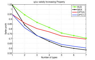
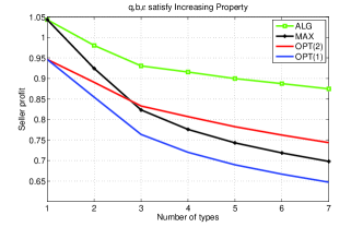
Our observations are as follows. Being able to use more contracts is always better as expected (i.e., OPT(1) $\leq$ OPT(2) in all cases). When the monotonicity condition holds, ALG is optimal and thus outperforms all other algorithms. When $K=1,2$ OPT(2) should have been optimal but it falls below ALG due to the discretization error. When $K>2$, ALG further has the advantage of being able to use more than $2$ contracts. Recall that MAX is the optimal contract when the seller knows exactly the type; thus, MAX is optimal when $K=1$ and outperforms exhaustive search because it does not suffer from discretization error. In the general case when the monotonicity does not necessarily hold, although ALG is not always optimal it still outperforms both OPT(1) and OPT(2). Finally, when the buyer type is harder to predict (as $K$ increases), the maximum expected profit decreases.

VIII Conclusion

We considered a contract design problem where a primary license holder wishes to profit from its excess spectrum capacity by selling it to potential secondary users/buyers via designing a set of profitable contracts. We completely characterize the optimal solution in the cases where there is a single buyer type, and when multiple types of buyers share a common, known channel condition. In the case when each type of buyers have different channel conditions we construct an algorithm that generates a set of contracts in a computationally efficient manner, and show that this set is optimal when the buyer types satisfy a monotonicity condition.

Theorem. 9

Proof.

Case 1

$x^{\prime}\leq x_{i}^{*}\leq x_{j}^{*}$
When $x^{\prime}\leq x_{i}^{*}$ and $x^{\prime}\leq x_{j}^{*}$, the equal cost lines for $x<x^{\prime}$ are of the form,

$$P_{i}(x^{\prime},p^{\prime},x)=b_{i}-\frac{q_{i}-\epsilon_{i}-\delta_{i}}{x}$$

$$P_{j}(x^{\prime},p^{\prime},x)=b_{j}-\frac{q_{j}-\epsilon_{j}-\delta_{j}}{x}$$

where we let $\delta_{i}=C_{i}(x^{\prime},p^{\prime})$ and $\delta_{j}=C_{j}(x^{\prime},p^{\prime})$. Take the derivatives with respect to $x$.

$$\frac{\partial P_{i}(x^{\prime},p^{\prime},x)}{\partial x} = (q_{i}-\epsilon_{i}-\delta_{i})x^{-2}$$

$$\frac{\partial P_{j}(x^{\prime},p^{\prime},x)}{\partial x} = (q_{j}-\epsilon_{j}-\delta_{j})x^{-2}$$

By definition, $P_{i}(x^{\prime},p^{\prime},x^{\prime})=p^{\prime}=P_{j}(x^{\prime},p^{\prime},x^{\prime})$,

$$p^{\prime}=b_{i}-\frac{q_{i}-\epsilon_{i}-\delta_{i}}{x^{\prime}}=b_{j}-\frac{q_{j}-\epsilon_{j}-\delta_{j}}{x^{\prime}}$$

Considering $b_{i}<b_{j}$, we know that $q_{j}-\epsilon_{j}-\delta_{j}>q_{i}-\epsilon_{i}-\delta_{i}$. Which implies $\frac{\partial P_{j}(x^{\prime},p^{\prime},x)}{\partial x}\geq\frac{\partial P_{i}(x^{\prime},p^{\prime},x)}{\partial x}$, and thus $P_{i}(x^{\prime},p^{\prime},x)\geq P_{j}(x^{\prime},p^{\prime},x)$, $\forall x<x^{\prime}$.

Case 2

$x_{i}^{*}\leq x^{\prime}\leq x_{j}^{*}$
The equal cost lines are,

$$P_{i}(x^{\prime},p^{\prime},x) = \left\{\begin{tabular}[]{ll}$\frac{x^{\prime}p^{\prime}}{x}$&$x_{i}^{*}\leq x\leq x^{\prime}$\\ $b_{i}-\frac{q_{i}-\epsilon_{i}-\delta_{i}}{x}$&$x\leq x_{i}^{*}$\end{tabular}\right.$$

$$P_{j}(x^{\prime},p^{\prime},x) = b_{j}-\frac{q_{j}-\epsilon_{j}-\delta_{j}}{x} ~{}~{}x\leq x^{\prime}$$

Where $\delta_{i}=C_{i}(x^{\prime},p^{\prime})$ and $\delta_{j}=C_{j}(x^{\prime},p^{\prime})$. Taking the derivatives,

$$P^{\prime}_{i}(x^{\prime},p^{\prime},x) = \left\{\begin{tabular}[]{ll}$-x^{\prime}p^{\prime}x^{-2}<0$&$x^{i*}\leq x\leq x^{\prime}$\\ $(q_{i}-\epsilon_{i}-\delta_{i})x^{-2}>0$&$x\leq x^{i*}$\end{tabular}\right.$$

$$P^{\prime}_{j}(x^{\prime},p^{\prime},x) = (q_{j}-\epsilon_{j}-\delta_{j})x^{-2}>0 ~{}~{}x\leq x^{\prime}$$

This implies $P_{i}(x^{\prime},p^{\prime},x)>P_{j}(x^{\prime},p^{\prime},x)$, $\forall x$ $x_{i}^{*}\leq x\leq x^{\prime}$.

$$P_{i}(x^{\prime},p^{\prime},x_{i}^{*}) = b_{i}-\frac{q_{i}-\epsilon_{i}-\delta_{i}}{x_{i}^{*}}$$

$$> P_{j}(x^{\prime},p^{\prime},x_{i}^{*})=b_{j}-\frac{q_{j}-\epsilon_{j}-\delta_{j}}{x_{i}^{*}}$$

Since $b_{i}<b_{j}$, we conclude that $q_{j}-\epsilon_{j}-\delta_{j}\geq q_{i}-\epsilon_{i}-\delta_{i}$. Which indicates that $\frac{\partial P_{j}(x^{\prime},p^{\prime},x)}{\partial x}\geq\frac{\partial p_{i}(x^{\prime},p^{\prime},x)}{\partial x}$ and $P_{i}(x^{\prime},p^{\prime},x)\geq P_{j}(x^{\prime},p^{\prime},x)$, $\forall x\leq x_{i}^{*}$.

Case 3

$x^{\prime}\geq x_{j}^{*}\geq x_{i}^{*}$
When $x\geq x_{j}^{*}\geq x_{i}^{*}$, the equal cost line of both types follow $x^{\prime}p^{\prime}=xp$. Thus, $P_{i}(x^{\prime},p^{\prime},x_{j}^{*})=P_{j}(x^{\prime},p^{\prime},x_{j}^{*})$. Then the case falls into Case 2 and $P_{i}(x_{j}^{*},P_{j}(x^{\prime},p^{\prime},x_{j}^{*}),x)\geq P_{j}(x_{j}^{*},P_{j}(x^{\prime},p^{\prime},x_{j}^{*}),x)$, $\forall x<x_{j}^{*}$.

∎

Theorem. 8

Proof.

Case 1

$x^{\prime}\leq x_{i}^{*}\leq x_{j}^{*}$
When $x^{\prime}\leq x_{i}^{*}\leq x_{j}^{*}$, both types have equal utiliy line of the same form.

$$P_{i}(x^{\prime},p^{\prime},x)=b_{i}-\frac{q_{i}-\epsilon_{i}-C_{i}(x^{\prime},p^{\prime})}{x}$$

$$P_{i}(x^{\prime},p^{\prime},x)=b_{j}-\frac{q_{j}-\epsilon_{j}-C_{j}(x^{\prime},p^{\prime})}{x}$$ (18)

By exactly the same argument as in Theorem. 9 we can find out that. $\frac{\partial P_{j}(x^{\prime},p^{\prime},x)}{\partial x}\geq\frac{\partial p_{i}(x^{\prime},p^{\prime},x)}{\partial x}$, and thus,

$$P_{i}(x^{\prime},p^{\prime},x)\leq P_{j}(x^{\prime},p^{\prime},x)~{}\forall x_{i}^{*}\geq x\geq x^{\prime}$$

When $x_{i}^{*}<x<x_{j}^{*}$, while $P_{j}(x^{\prime},p^{\prime},x)$ still follows the same formula (Equation. 18), $P_{i}(x^{\prime},p^{\prime},x)$ starts to decrease by following the line $P_{i}(x^{\prime},p^{\prime},x)=x^{\prime}P_{i}(x^{\prime},p^{\prime},x_{i}^{*})/x$. Thus,

$$P_{i}(x^{\prime},p^{\prime},x)\leq P_{j}(x^{\prime},p^{\prime},x)~{}\forall x_{i}^{*}\leq x\leq x_{j}^{*}$$

When $x>x_{j}^{*}$, both $i,j$ follow the form $P(x^{\prime},p^{\prime},x)=P(x^{\prime},p^{\prime},x_{j}^{*})/x$. But $P_{i}(x^{\prime},p^{\prime},x_{j}^{*})\leq P_{j}(x^{\prime},p^{\prime},x_{j}^{*})$, they never cross and $P_{j}(x^{\prime},p^{\prime},x)\geq P_{i}(x^{\prime},p^{\prime},x)$ $\forall x>x_{j}^{*}$.

Case 2

$x_{i}^{*}<x^{\prime}<x_{j}^{*}$
When $x_{i}^{*}<x^{\prime}<x<x_{j}^{*}$ they are of the form,

$$P_{i}(x^{\prime},p^{\prime},x) = \frac{x^{\prime}p^{\prime}}{x}$$

$$P_{j}(x^{\prime},p^{\prime},x) = b_{j}-\frac{q_{j}-\epsilon_{j}-C_{j}(x^{\prime},p^{\prime})}{x}$$

respectively. By the same argument as in Theorem. 9, $P_{i}$ is decreasing while $P_{j}$ is increasing. Thus, $P_{i}(x^{\prime},p^{\prime},x_{j}^{*})\leq P_{j}(x^{\prime},p^{\prime},x_{j}^{*})$. When $x>x_{j}^{*}$,

$$P_{i}(x^{\prime},p^{\prime},x)=\frac{x_{j}^{*}P_{i}(x^{\prime},p^{\prime},x_{j}^{*})}{x}$$

$$P_{j}(x^{\prime},p^{\prime},x)=\frac{x_{j}^{*}P_{j}(x^{\prime},p^{\prime},x_{j}^{*})}{x}$$

Since $P_{i}(x^{\prime},p^{\prime},x_{j}^{*})<P_{j}(x^{\prime},p^{\prime},x_{j}^{*})$ we konw that $P_{i}(x^{\prime},p^{\prime},x)<P_{j}(x^{\prime},p^{\prime},x)$ $\forall x>x_{j}^{*}$.

Case 3

$x^{\prime}>x_{j}^{*}>x_{i}^{*}$
When $x>x_{j}^{*}$, both types have equal cost line as $xp=x^{\prime}p^{\prime}$. Thus, $P_{i}(x^{\prime},p^{\prime},x)=P_{j}(x^{\prime},p^{\prime},x)$ $\forall x>x_{j}^{*}$.

∎

References

- [1] I.F. Akyildiz, W.Y. Lee, M.C. Vuran, and S. Mohanty. Next generation/dynamic spectrum access/cognitive radio wireless networks: a survey. Computer Networks, 50(13):2127–2159, 2006.
- [2] M.M. Buddhikot. Understanding dynamic spectrum access: Models, taxonomy and challenges. In New Frontiers in Dynamic Spectrum Access Networks, 2007. DySPAN 2007, pages 649–663. IEEE, 2007.
- [3] Y. Wu, B. Wang, K. Liu, and T.C. Clancy. A multi-winner cognitive spectrum auction framework with collusion-resistant mechanisms. In New Frontiers in Dynamic Spectrum Access Networks, 2008. DySPAN 2008. 3rd IEEE Symposium on, pages 1–9. IEEE, 2008.
- [4] S. Gandhi, C. Buragohain, L. Cao, H. Zheng, and S. Suri. A general framework for wireless spectrum auctions. In New Frontiers in Dynamic Spectrum Access Networks, 2007. DySPAN 2007. 2nd IEEE International Symposium on, pages 22–33. IEEE, 2007.
- [5] J. Huang, R.A. Berry, and M.L. Honig. Auction-based spectrum sharing. Mobile Networks and Applications, 11(3):405–418, 2006.
- [6] V. Grimm, F. Riedel, and E. Wolfstetter. Low price equilibrium in multi-unit auctions: the gsm spectrum auction in germany. International journal of industrial organization, 21(10):1557–1569, 2003.
- [7] H. Kim and K. G. Shin. Efficient discovery of spectrum opportunities with mac-layer sensing in cognitive radio networks. IEEE Transactions on Mobile Computing, 7(5):533–545, May 2008.
- [8] X. Liu and S. Shankar N. Sensing-based opportunistic channel access. Journal of Mobile Networks and Applications, August 2006.
- [9] Q. Zhao, L. Tong, A. Swami, and Y. Chen. Decentralized cognitive mac for opportunistic spectrum access in ad hoc networks: A pomdp framework. IEEE Journal on Selected Areas in Communications (JSAC), 5(3):589–600, April 2007.
- [10] S. H. A. Ahmad, M. Liu, T. Javidi, Q. Zhao, and B. Krishnamachari. Optimality of myopic sensing in multi-channel opportunistic access. IEEE Transactions on Information Theory, September 2009.
- [11] L. Duan, L. Gao, and J. Huang. Contract-based cooperative spectrum sharing. In Dynamic Spectrum Access Networks (DySPAN), 2011.
- [12] P.K. Muthuswamy, K. Kar, A. Gupta, S. Sarkar, and G. Kasbekar. Portfolio optimization in secondary spectrum markets. In WiOpt, 2011.
- [13] http://www-personal.umich.edu/~shangpin/Full_Version.pdf.
- [14] T.H. Cormen. Introduction to algorithms. The MIT press, 2001.
- [15] X. Wang, A. Montgomery, and K. Srinivasan. When auction meets fixed price: a theoretical and empirical examination of buy-it-now auctions. Quantitative Marketing and Economics, 6(4):339–370, 2008.
- [16] R. Zeithammer and P. Liu. When is auctioning preferred to posting a fixed selling price? University of Chicago, 2006.
- [17] R.B. Myerson. Optimal auction design. Mathematics of operations research, pages 58–73, 1981.
- [18] P. Auer, R. Ortner, and C. Szepesvári. Improved rates for the stochastic continuum-armed bandit problem. Learning Theory, 2007.
- [19] P. Auer, N. Cesa-Bianchi, and P. Fischer. Finite-time analysis of the multiarmed bandit problem. Machine learning, 47(2):235–256, 2002.
Theorem. 9
Proof.
- Case 1
-
When and , the equal cost lines for are of the form,where we let and . Take the derivatives with respect to .
By definition, ,
Considering , we know that . Which implies , and thus , .
- Case 2
The equal cost lines are,Where and . Taking the derivatives,
This implies , .
Since , we conclude that . Which indicates that and , .
- Case 3
When , the equal cost line of both types follow . Thus, . Then the case falls into Case 2 and , .
∎
Theorem. 8
When , both types have equal utiliy line of the same form.(18) By exactly the same argument as in Theorem. 9 we can find out that. , and thus,
When , while still follows the same formula (Equation. 18), starts to decrease by following the line . Thus,
When , both follow the form . But , they never cross and .
When they are of the form,respectively. By the same argument as in Theorem. 9, is decreasing while is increasing. Thus, . When ,
Since we konw that .
When , both types have equal cost line as . Thus, .