Optimal reconstruction of the folding landscape using differential energy surface analysis
Abstract
In experiments and in simulations, the free energy of a state of a system can be determined from the probability that the state is occupied. However, it is often necessary to impose a biasing potential on the system so that high energy states are sampled with sufficient frequency. The unbiased energy is typically obtained from the data using the weighted histogram analysis method (WHAM). Here we present differential energy surface analysis (DESA), in which the gradient of the energy surface, , is extracted from data taken with a series of harmonic biasing potentials. It is shown that DESA produces a maximum likelihood estimate of the folding landscape gradient. DESA is demonstrated by analyzing data from a simulated system as well as data from a single-molecule unfolding experiment in which the end-to-end distance of a DNA hairpin is measured. It is shown that the energy surface obtained from DESA is indistinguishable from the energy surface obtained when WHAM is applied to the same data. Two criteria are defined which indicate whether the DESA results are self-consistent. It is found that these criteria can detect a situation where the energy is not a single-valued function of the measured reaction coordinate. The criteria were found to be satisfied for the experimental data analyzed, confirming that end-to-end distance is a good reaction coordinate for the experimental system. The combination of DESA and the optical trap assay in which a structure is disrupted under harmonic constraint facilitates an extremely accurate measurement of the folding energy surface.
pacs:
87.14.G-,87.15.Cc,87.15.hmI Introduction
In a dynamical system driven by thermal fluctuations the effective energy as a function of conformation is related to the probability that the conformation is observed by the Boltzmann formula,
| (1) |
where is the Boltzmann constant and is the temperature. The conformation of a simple system may be specified by a small number of variables. However, in studies of the folding of bio-polymers the conformational space of the system has many degrees of freedom. In some cases, such systems can be described in terms of a single reaction coordinate, , and the dynamics of the system can be modeled by diffusion in this 1D space under the influence of an effective energyPlotkin and Onuchic (2002); Onuchic and Wolynes (2004); Wolynes et al. (1995); Dill et al. (2008). In numerical simulations the reaction coordinate may be the radius of gyration of the structure, the fraction of native contacts, or another measure of the level of compaction or organization of the molecule. In single molecule manipulation experiments the end-to-end extension of the molecule is typically used as a reaction coordinateLiphardt et al. (2001). The energy as a function of the reaction coordinate follows from Eq. 1 as
| (2) |
The arbitrary constant is included because the energy of a system is only defined up to a additive constant. Although this formula can be used, in principle, to determine the energy surface from the probability density function, this is only practical when the energy varies in a range which is narrow compared with . The exponential dependence of the probability density on means that states with relative energy that is large compared with will be impossible to sample in a finite time.
One solution to this problem is to apply an external force field to the system which tends to bias it towards the regions of the reaction coordinate that would otherwise be poorly sampled. Often, this takes the form of a harmonic constraint, which adds an additional term to the energy, where is the effective stiffness and is the origin of the constraint. By selecting an appropriate value of and varying , the system can be forced to visit various regions of the reaction coordinate, allowing more uniform convergence of statistics. This technique, often referred to as umbrella samplingTorrie and Valleau (1974), is widely used in simulationsFrenkel and Smit (2003), and has been applied to single molecule experimentsde Messieres et al. (2011).
We can still apply Eq. 2 to the system with a specific configuration of the harmonic constraint, but we will obtain a biased energy which is the sum of the intrinsic energy and the energy of the constraint. To find the unbiased energy, we subtract the known constraint energy, and obtain
| (3) |
For each position of the constraint we obtain a measurement of the energy surface over the region visited by the system. Each local energy surface contains an independent constant .
If we wish to find the global energy surface, defined over the entire domain of , we need to choose the constants and combine the local energy landscapes in a self-consistent manner. If there is substantial overlap between the domains of the local landscapes, the constants can be determined by requiring that the energy surfaces corresponding to different constraints are consistent in the overlap regions.
The weighted histogram analysis method (WHAM) has been formulated to reconstruct the energy surface from Monte Carlo or molecular dynamics simulations with arbitrary biasing potentialsKramers (1940); Ferrenberg and Swendsen (1989); Kumar et al. (1992); Boczko and Brooks (1995). The method provides an optimal estimate for the unbiased probability density ,
| (4) |
where is the probability density sampled in biased simulation and the summation is over all simulations. In the case of a harmonic constraint centered at , the weights are given by
| (5) |
where is the total number of measurements in simulation . The constants are defined implicitly by a system of nonlinear equations,
| (6) |
where the histogram count is the number of measurements between and in system , and is related to the probability by .
In the following section, we describe another method of obtaining the global energy surface which we call differential energy surface analysis (DESA). In DESA, we consider the slope of the energy landscape, rather than the energy itself. Differentiating Eq. 3 with respect to we obtain
| (7) |
An important feature of this equation is that the constants are eliminated, so that it is not necessary to find a self-consistent solution to obtain the global function . At any given point along the landscape, can be obtained by averaging obtained from the system at various constraint origins.
II Description of DESA
In order to define the method of differential energy landscape analysis, we assume a thermally driven system with one reaction coordinate which is characterized by an energy function . We assume that the dynamics of the system are measured in the presence of a harmonic constraint of stiffness for distinct constraint origins . For each , the time series of is used to compile a histogram containing total samples. We assume that the histogram binning is consistent for all , and that the values of and are chosen so that there is significant overlap between the histograms. The slope of the energy landscape at position is given by
| (8) |
where the summation is over the constraint origins, , and is defined by Eq. 7. Interpreting this formula, the value of at position is a weighted average of found from the systems with constraint origins . Using , we can express Eq. 8 entirely in terms of histogram counts, as
| (9) | |||||||
This formula has been used to reconstruct energy landscapes of molecular dynamics simulationsDenesyuk and Weeks (2009), and experimental datade Messieres et al. (2011). We will show below that Eq. 9 gives an optimal estimation of .
When determining the mean value of a Gaussian distributed variable from uncorrelated data points which have differing uncertainty, the maximum likelihood solution is
| (10) |
where is the standard deviation of the statistical ensemble from which is taken, is the mean of and is the standard deviation of . In order to show that Eq. 8 is a maximum likelihood estimate of we must show that the choice meets the criteria set out in Eq. 10.
Starting with Eq. 7, the evaluation of will involve a finite difference of the natural logarithm of ,
| (11) | |||||
where represents the statistical uncertainty in , and . Note that any terms with are suppressed in Eq. 8, but we also must suppress any terms where or is zero, since in this case the derivative is undefined. We can re-express Eq. 11 as
| (12) | |||||
so that the uncertainties in and produce additive uncertainties in . Assuming the uncertainty in is statistical, the uncertainty terms can be simplified using , so that
| (13) |
where the last step is an expansion of the expression to first order. Since and are uncorrelated, the errors arising from these terms add in quadrature. In the limit that is small compared with any important features of the energy landscape we can neglect the difference between and , and replace both by . Using Eq. 13 we can then approximate the uncertainty in as
| (14) |
The statistical weight required for maximum likelihood is therefore
| (15) |
Since an overall multiplicative factor will cancel out in Eq. 10 and not affect the calculation of the mean value, Eq. 8 is equivalent to the maximum likelihood estimation of and is an optimal estimation.
III Diagnostics in the DESA method
Recent work has provided criteria for error estimation in free energy calculations based on the weighted histogram analysis methodZhu and Hummer (2011); Chodera et al. (2007). The DESA result is obtained by straightforward averaging of estimates obtained with different constraint origins . Use of the maximum likelihood estimation assures that the optimal value of is produced, and straightforward error propagation can be used to obtain the uncertainty in the values of obtained. However, when employing umbrella sampling, it is necessary to assume that the histograms obtained for different constraint origins overlap and that the data acquired with different constraint origins are sampling the same energy surface. One potential pitfall of umbrella sampling—whether WHAM or DESA is used for analysis of the data—is that we can obtain a smooth measured energy surface even if the energy is not a single-valued function of the reaction coordinate. Here we introduce two criteria that can be applied in order to detect inconsistencies in values obtained from different constraint origins. We will later show that these criteria give a warning when the reconstructed landscape is not accurate.
The first method involves comparison of the biased energy surfaces obtained from different constraint origins. Subtracting two biased energies, we obtain
| (16) | |||||||
where is the biased energy surface measured with constraint origin and is the unbiased energy of the system. The cancelation of leaves terms which depend only on the biasing potential. The constant term is not of interest, since the energy itself is only defined up to an additive constant. However, we expect the energy difference to manifest a straight line with slope determined by the constraint strength and the relative constraint displacement, . If a different effective energy surface is in effect after the constraint origin bas been moved, will fail to cancel in Eq. 16 and anomalous features will appear in the difference curve.
We can also test the self-consistency of the DESA analysis by determining if values obtained from individual constraint origins deviate from the mean value in a manner that is consistent with their statistical uncertainty. For each histogram bin corresponding to position , we evaluate
| (17) |
where is the uncertainty in the value of obtained from the constraint position (Eq. 14). If the deviation of the individual values of from the mean are consistent with the statistical uncertainty, the value of should be of order 1. A value significantly larger than 1 indicates that systematic errors are present in the values.
IV Application of DESA to a simulated system
WHAM produces an optimal estimation of which is closely related to the energy and DESA produces an optimal estimation of . For a well-behaved system with good statistical convergence we expect both methods to converge to the underlying energy surface. However, in simulations and in experiments it is often a challenge to obtain adequate statistics, or obtain a reaction coordinate which unambiguously specifies the state of the system.
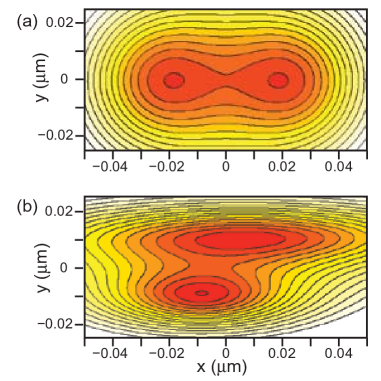
In Section V below we will apply DESA and WHAM to an experimental system and compare the results. In this section we will apply DESA and WHAM to two simulated systems in order to evaluate the accuracy with which the known energy surface is obtained and illustrate the use of the diagnostic criteria that were introduced in Section III. Both simulated systems involved diffusion on a 2D energy surface with two stable states and in both cases we assume that only one coordinate () is measured and that the biasing potential is a function of only. Contour maps for the potential functions for the two systems are shown in Fig. 1. For both cases, the landscape consists of two overlapping potential wells with 2-dimensional Lorentzian profile. The form of the potential is
| (18) | |||||
where specifies the depth of each well, (, ) specifies the center and (, ) specifies the width of each well in the and direction.
In system I, illustrated by Fig. 1(a), there are two symmetrical potential wells lying on the axis (parameters given in the Fig. 1 caption). For this potential there is only one stable value of for each . In system II, illustrated by Fig. 1(b) the two potential wells have different width and are displaced in as well as . In system II there is more than one stable value of for a given value of and the measurement of is not sufficient to determine the state of the system. The transition between the two stable states of the system involves a change in the unmeasured variable . Both simulated systems could serve as a model for a single-molecule unfolding experiment (such as the one described in Section V) where a quantity such as the end-to-end distance of the structure is under experimental control but other undetectable degrees of freedom are present. In system I, the measured variable is a good reaction coordinate and in the system II it is not.
The energy surfaces are used as the basis of a strongly damped Langevin simulation with thermal energy and drag coefficient . In the simulation 400 time steps of were taken between each tabulated sample point. These parameters were chosen so that the energy and time scales of the simulated systems roughly correspond to those of the experimental system which we describe in Section V. As a result, simulated and experimental runs of equal time result in comparable statistical sampling. Both simulation systems are run with a harmonic biasing potential which is continuously swept from negative to positive to sample the transition. In system I the constraint stiffness is 150 pN/nm and the constraint origin sweeps from -0.03 m to 0.03 m over 4 s and in system II the stiffness is 100 pN/nm and the origin sweeps the same range of position.
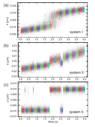
The trajectories obtained for the two versions of the simulation are shown in Fig. 2. In system I, the biasing potential causes the system to be swept through the transition state with good sampling over the domain of the reaction coordinate . (In the course of the transition, fluctuates around zero, data not shown.) In system II, the biasing potential also produces relatively uniform sampling of , although makes several abrupt transition between the basins of attraction at (-0.009 m,-0.011 m) and (0.009 m,0.011 m). The potential well at positive is more extended in than the one at negative , resulting in larger fluctuations in when is positive.
The record of vs. time of the trajectories is divided into 20 equal time intervals and the histogram of position is calculated for each interval. Data for each division is analyzed using the constant constraint stiffness and the average position of the constraint origin. In this simulation, it would be more natural to move the constraint origin in discrete steps and hold it constant as each histogram is collected. We move it continuously to more closely model the experimental procedure used in the experiment described in Section V. In order to apply DESA or WHAM the constraint must be moved sufficiently slowly that the system remains in quasi-equilibrium with respect to as the constraint origin moves. We have chosen the simulation parameters to ensure that this condition is satisfied for both systems.
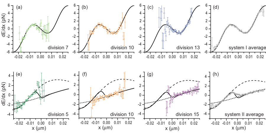
In Fig. 3 the reconstruction of from the simulated systems is shown. In Fig. 3(a)-(c) Eq. 7 is used to obtain an estimation of from three representative divisions of the system I trajectory. The three curves cover overlapping ranges of the reaction coordinate . The curve obtained from each division exhibits good statistical convergence in center of its domain and poorer statistical convergence at the margins. Within statistical uncertainty, the curves are consistent with the potential used in the simulation and with each other. When the 20 curves obtained from the 20 divisions are combined using Eq. 9 good agreement is found between the reconstructed shown in Fig. 3(d) and the energy surface used in the simulation.
When the same analysis is applied to system II the DESA method provides a visual indication that the dynamics of the system are not described by an energy which can be expressed as a function of a single reaction coordinate . In Fig. 2(e)-(g) estimates from three divisions of the trajectory are shown. They are compared with derivative of the system energy with respect to , assuming that the system remains in equilibrium with respect to (solid curve), assuming that the system is confined to negative (dashed curve) and assuming that the system is confined to positive (short dashed curve). The estimate of obtained from division 5 conforms to the potential for negative while the estimate from divisions 10 and 15 conform to the potential for positive . The reconstructed curve shown in Fig. 3(h) gives a smooth curve despite the fact that it is obtained from averaging of inconsistent functions.
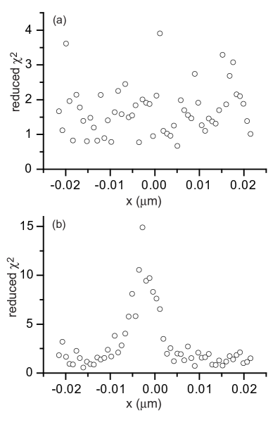
We next apply the DESA diagnostics introduced in Section III. In Fig. 4 the reduced test defined in Eq. 17 is applied to both simulated systems. The purpose of this test is to determine if the values of obtained from the various divisions of the data are consistent with each other, taking into account the statistical uncertainties of the various estimates. Fig. 4(a) shows that for system I the reduced is of order 1 over the full range of . This indicates that the functions obtained for the different constraint origins are mutually consistent. However, Fig. 4(b) shows that for system II the value of the reduced function increases to 15 in the vicinity of the apparent transition state. This confirms our observation that in Fig. 3(e)-(g) the functions deviate from each other by an amount exceeding the statistical uncertainty. This alerts us that data obtained from different biasing potentials are not consistent and is not a well defined function of , despite the fact that the curve obtained is smooth and appears plausible.
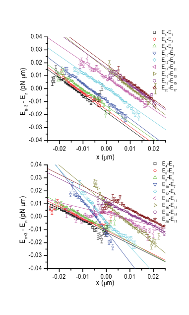
Next we consider the diagnostic criteria defined in Eq. 16, in which we subtract the raw energy surfaces obtained from data taken with different biasing potentials. In Fig. 5(a), Eq. 16 is evaluated for representative divisions of the data from system I. Linear curves are found with slopes that are consistent with the constraint stiffness used in the simulation. In Fig. 5(b) the same measure is applied to representative divisions from system II. Inconsistent slopes, or non-linear curves are observed. This indicates that the intrinsic energy surface of the system failed to cancel when the energy surfaces of different divisions were subtracted. As in the case of Fig. 4, it is evident that the data produced by the simulation of system II are not self-consistent.
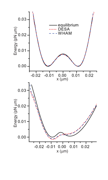
The final question we can address is whether DESA or WHAM are more accurate in determining the relative energy of the initial and final states for the two systems. In Fig. 6 we compare the energy surfaces obtained by direct integration of the DESA curve, and using WHAM. In the case of the well-behaved system I (Fig. 6(a)), both DESA and WHAM produce energy curves which match the potential used in the simulation. In the case of system II (Fig. 6(b)) we find that DESA and WHAM produce energy curves which are effectively identical. Both curves fail to agree with the actual energy difference between the initial and final state. In this example, the energy surface was known a priori making direct comparison possible. However, the diagnostic criteria illustrated in Fig. 4 and 5 alerted us to problems in the reconstruction of the energy surface and did not require knowledge of the correct energy surface.
V Application of DESA to experimental data
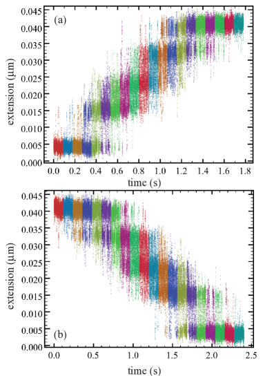
Here we apply DESA and WHAM to a single molecule experiment in which a DNA hairpin is unfolded under a harmonic constraint applied by an optical trap. The hairpin has sequence CCGCGAGTTGATTCGCCATACACCTGCTAATCCCGGTCGCTTTTGCGACCGGGATTAGCAGGTGTATGGCGAATCAACTCGCGG, which folds into a 40 base-pair stem with a 4-T loop. The hairpin is connected to the boundary of the sample chamber on one side and to a polystyrene micro-sphere on the other via biotin and digoxigenin tagged double-stranded DNA linkers. This creates a single-molecule tether which anchors the micro-sphere to the surface. When the optical trap is held at constant position and intensity, the combination of the restoring force imposed on the micro-sphere by the optical trap and the elasticity of the handles produce a harmonic constraint acting on the hairpin with . The position of the sample chamber relative to the trapping beam is controlled by a piezoelectric positioning stage with nanometer resolution, and the origin of the constraint is controlled by varying the position of the sample chamber with respect to the trap center. The optical trap measures the instantaneous position of the micro-sphere and the instantaneous force applied to the tether as the constraint origin is swept. By determining the distance between the micro-sphere and the sample chamber boundary and subtracting off the instantaneous extension of the double-stranded DNA handles (estimated using a worm-like chain model of DNA elasticity) the extension of the hairpin itself is determinedMarko and Siggia (1995). The apparatus and experimental procedure has been described elsewherede Messieres et al. (2011). The measured time series comprised of approximately samples is shown for unfolding of the hairpin in Fig. 7(a), and for folding of the hairpin in Fig. 7(b).
As in the case of the simulated data, the record of extension vs. time of the experimental system is divided into 20 equal time intervals and the histogram of position is calculated for each division. Calibration data is used to calculate the mean stiffness and origin of the constraint for each of the 20 divisionsde Messieres et al. (2011). Since the constraint origin moves continuously as data is acquired, it is not a constant within each interval. However, the deviation of the constraint origin from the mean value does not exceed 1 nm in the course of an interval, which implies an error in the constraint force of less than 0.2 pN. The resulting error in the reconstruction of is negligible.
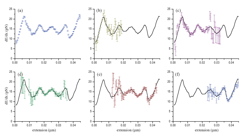
In Fig. 8 the functions calculated from representative divisions of the data in Fig. 7(a) are shown in panels (b) through (f) and the function obtained by averaging all 20 divisions is shown in panel (a). Just as in Fig. 3(a)-(c), the individual estimates in Fig. 8 are consistent with each other and with the average function within statistical uncertainty. This justifies the assumption that the experimental system continues to explore the same energy landscape as the constraint origin moves.
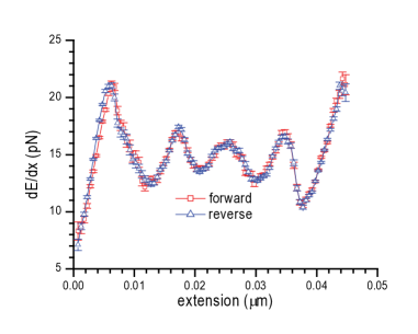
As in the simulated system, the umbrella sampling method requires us to assume that the biasing potential is time independent and that the system remains in thermodynamic equilibrium as data is collected. Since the constraint origin moves continuously as data is collected this condition is not formally satisfied, and we must insure that the movement of the constraint is sufficiently slow that the system remains in equilibrium to good approximation. The most convincing evidence that this condition is satisfied is that identical energy landscapes are obtained for folding and unfolding of the hairpin, for which the constraint origin moves in opposite directions. The energy landscapes obtained from data in Figs. 7(a) and 7(b) are compared in Fig. 9. No significant difference is found between landscapes obtained for folding and unfolding of the hairpin.
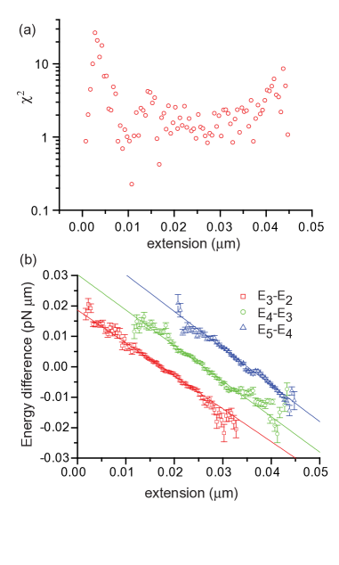
In contrast with the simulations, the effective energy of the hairpin is not known a priori so the diagnostic criteria introduced in Section III are of critical importance in establishing the validity of the energy landscape reconstruction. In Fig. 10 we apply the two diagnostic criteria defined in Section III to the experimental data set. In Fig. 10(a) the measure is plotted on a logarithmic scale. Note that for the central region of the reaction coordinate, corresponding to the transition state, the value of is of order unity, which indicates that the curves obtained in the transition state region are consistent within statistical uncertainty. This confirms that a well-defined energy function is being measured. At the extremes (near extension 0 m and 0.05 m) the value of is larger, indicating that the curves are inconsistent at large and small extension.
The larger values are found in regimes of extension where the hairpin is either fully open or fully folded. When the constraint is positioned to stabilize the hairpin in the fully open or fully closed conformation, the conformational dynamics of the hairpin itself are minimal and the fluctuations in the measured extension are mainly due to thermal fluctuation in the extension of the double-stranded DNA handles. At small extensions, the problem is exacerbated by the fact that the average force is low, resulting in lower effective stiffness of the handles and increased fluctuations. These measurement errors blur the sharp cutoff that would otherwise appear in the probability density of extension as the hairpin approaches the fully-open or fully-folded state and similarly blur the energy function. The function alerts us to the fact that the energy surface is accurately measured in the transition state region, but is affected by systematic errors near the fully folded or fully unfolded state.
We also apply the criterion based on Eq. 16 and show the results in Fig. 10(b). The fact that linear curves are obtained when the unbiased energies are subtracted indicate that the intrinsic energy of the hairpin cancels, as expected, and that the effective biasing potential has the expected parabolic shape. This is confirmation that the optical trapping apparatus is applying an accurate biasing potential to the hairpin. Based on Fig. 10 we conclude that the energy of the hairpin is a well-defined function of extension and that DESA has produced an accurate measurement of the transition state region.
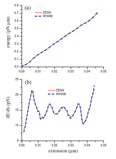
In order to verify the DESA result, the data shown in Fig. 7 was also analyzed using WHAM, as defined by Eqs 5 and 6. In Fig. 11(a) the energy surface obtained by WHAM is plotted along with the energy surface obtained from integration of the curve shown in Fig. 8. The DESA and WHAM curves are indistinguishable. The overall slope of the energy landscape is reproduced, as well as the ripples that arise from the sequence dependence of the DNA hybridization energy. The sequence dependence is more apparent in the plot of , which is shown in Fig. 11(b). As in the case of the energy, results obtained from DESA and WHAM are indistinguishable.
VI Conclusions
There are systems, such as pseudoknots, G-quadruplex DNA and others, which exhibit large irreversible steps when disrupted in single molecule experimentsGreen et al. (2008); Yu et al. (2009); de Messieres et al. (2012). In such cases, the techniques described here would not be suitable for reconstructing the global energy landscape. The main obstacle is that it is impossible to apply a biasing potential which will stabilize the system in the transition state or states. Both WHAM and DESA require that the histograms of the reaction coordinate obtained with different biasing potentials have substantial overlap. Nonequilibrium analysis methods have been developed which can determine the energy surface from data taken far from equilibriumJarzynski (1997); Crooks (2000); Hummer and Szabo (2001, 2010); Evans (2001); Dudko et al. (2008). These methods typically require a great deal of experimental data, since they involve measuring the dependence of the disruption force on force loading rate or averaging many trajectories with weights determined by the external work performed.
In cases where biasing potentials can be used to stabilize a system along the reaction coordinate, DESA is an alternative to WHAM. We have shown that DESA and WHAM produce indistinguishable results when applied to simulated and experimental data. However, DESA has the advantage of being computationally simple compared with WHAM, which requires the self-consistent solution of a system of nonlinear equations (Eq. 6). Another advantage of DESA is that the construction of provides direct visual cues which can be used to confirm that the different biasing potentials are sampling the same energy surface (see Fig. 8). In addition, the two diagnostic criteria defined in Section III provide quantitative measures of the quality of the energy surface measurement. The signatures of an ill-defined energy surface are demonstrated in the analysis of data generated by simulation system II. Finally, using the DESA diagnostics, we show that it is possible to apply a precisely controlled biasing potential in an experimental system and obtain highly accurate information about the shape of the energy surface for folding and unfolding.
This work was supported by the Maryland Technology Development Corporation.
References
- Plotkin and Onuchic (2002) S. S. Plotkin and J. N. Onuchic, Quarterly Reviews of Biophysics 35, 111 (2002).
- Onuchic and Wolynes (2004) J. N. Onuchic and P. G. Wolynes, Current Opinion in Structural Biology 14, 70 (2004).
- Wolynes et al. (1995) P. G. Wolynes, J. N. Onuchic, and D. Thirumalai, Science 267, 1619 (1995).
- Dill et al. (2008) K. A. Dill, S. B. Ozkan, M. S. Shell, and T. R. Weikl, Annual Reviews of Biophysics 37, 289 (2008).
- Liphardt et al. (2001) J. Liphardt, B. Onoa, S. B. Smith, I. Tinoco, and C. Bustamants, Science 292, 733 (2001).
- Torrie and Valleau (1974) G. M. Torrie and J. P. Valleau, Chemical Physics Letters 28, 578 (1974).
- Frenkel and Smit (2003) D. Frenkel and B. Smit, Understanding Molecular Simulation (Academic Press, 2003).
- de Messieres et al. (2011) M. de Messieres, B. Brawn-Cinani, and A. La Porta, Biophysical Journal 100, 2736 (2011).
- Kramers (1940) H. A. Kramers, Physica VII, 284 (1940).
- Ferrenberg and Swendsen (1989) A. M. Ferrenberg and R. H. Swendsen, Physical Review Letters 63, 1195 (1989).
- Kumar et al. (1992) S. Kumar, J. M. Rosenberg, D. Bouzide, R. H. Swendsen, and P. A. Kollman, Journal of Computational Chemistry 13, 1011 (1992).
- Boczko and Brooks (1995) E. M. Boczko and C. L. Brooks, Science 269, 393 (1995).
- Denesyuk and Weeks (2009) N. A. Denesyuk and J. D. Weeks, Physical Review Letters 102, 108101 (2009).
- Zhu and Hummer (2011) R. Zhu and G. Hummer, Journal of Computational Chemistry 33, 453 (2011).
- Chodera et al. (2007) J. D. Chodera, W. C. Swope, J. W. Pitera, C. Seok, and K. A. Dill, Journal of Chemical Theory and Computation 3, 26 (2007).
- Marko and Siggia (1995) J. Marko and E. Siggia, Macromolecules 28, 8759 (1995).
- Green et al. (2008) L. Green, C.-H. Kim, C. Bustamante, and J. Tinoco, Ignacio, Journal of Molecular Biology 375, 511 (2008).
- Yu et al. (2009) Z. Yu, J. D. Schonhort, S. Dhakal, R. Bajracharya, R. Hegde, S. Basu, and H. Mao, Journal of the American Chemical Society 131, 1876 (2009).
- de Messieres et al. (2012) M. de Messieres, J.-C. Chang, B. Brawn-Cinani, and A. La Porta, Physical Review Letters 109, 058101 (2012).
- Jarzynski (1997) C. Jarzynski, Physical Review Letters 78, 2690 (1997).
- Crooks (2000) G. E. Crooks, Phys. Rev. E 61, 2361 (2000).
- Hummer and Szabo (2001) G. Hummer and A. Szabo, PNAS 98, 3658 (2001).
- Hummer and Szabo (2010) G. Hummer and A. Szabo, PNAS 107, 21441 (2010).
- Evans (2001) E. Evans, Annual Review of Biophysics and Biomolecular Structure 30, 105 (2001).
- Dudko et al. (2008) O. K. Dudko, G. Hummer, and A. Szabo, Proceedings of the National Academy of Science 105, 15755 (2008).