Optimal Sequential Wireless Relay Placement
on a Random Lattice Path

Abstract

Our work is motivated by the need for impromptu (or “as-you-go”) deployment of relay nodes (for establishing a packet communication path with a control centre) by firemen/commandos while operating in an unknown environment. We consider a model, where a deployment operative steps along a random lattice path whose evolution is Markov. At each step, the path can randomly either continue in the same direction or take a turn “North” or “East,” or come to an end, at which point a data source (e.g., a temperature sensor) has to be placed that will send packets to a control centre at the origin of the path. A decision has to be made at each step whether or not to place a wireless relay node. Assuming that the packet generation rate by the source is very low, and simple link-by-link scheduling, we consider the problem of relay placement so as to minimize the expectation of an end-to-end cost metric (a linear combination of the sum of convex hop costs and the number of relays placed). This impromptu relay placement problem is formulated as a total cost Markov decision process. First, we derive the optimal policy in terms of an optimal placement set and show that this set is characterized by a boundary beyond which it is optimal to place. Next, based on a simpler alternative one-step-look-ahead characterization of the optimal policy, we propose an algorithm which is proved to converge to the optimal placement set in a finite number of steps and which is faster than the traditional value iteration. We show by simulations that the distance based heuristic, usually assumed in the literature, is close to the optimal provided that the threshold distance is carefully chosen.

I Introduction

Wireless networks, such as cellular networks or multihop ad hoc networks, would normally be deployed via a planning and design process. There are situations, however, that require the impromptu (or “as-you-go”) deployment of a multihop wireless packet network. For example, such an impromptu approach would be required to deploy a wireless sensor network for situational awareness in emergency situations such as those faced by firemen or commandos (see [1, 2]). For example, as they attack a fire in a building, firemen might wish to place temperature sensors on fire-doors to monitor the spread of fire, and ensure a route for their own retreat; or commandos attempting to flush out terrorists might wish to place acoustic or passive infra-red sensors to monitor the movement of people in the building. As-you-go deployment may also be of interest when deploying a multi-hop wireless sensor network over a large terrain (such as a dense forest) in order to obtain a first-cut deployment which could then be augmented to a network with desired properties (connectivity and quality-of-service).

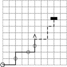
With the above larger motivation in mind, in this paper we are concerned with the rigorous formulation and solution of a problem of impromptu deployment of a multihop wireless network along a random lattice path, see Fig. 1. The path could represent the corridor of a large building, or even a trail in a forest. The objective is to create a multihop wireless path for packet communication from the end of the path to its beginning. The problem is formulated as an optimal sequential decision problem. The formulation gives rise to a total cost Markov decision process, which we study in detail in order to derive structural properties of the optimal policy. We also provide an efficient algorithm for calculating the optimal policy.

Figure 1: A wireless network being deployed as a person steps along a random lattice path. Inverted V: location of the deployment person; solid line: path already covered; circles: deployed relays; thick dashed path: a possible evolution of the remaining path. The sensor to be placed at the end is also shown as the black rectangle.

I-A Related Work

Our study is motivated by “first responder” networks, a concept that has been around at least since 2001. In [2], Howard et al. provide heuristic algorithms for the problem of incremental deployment of sensors (such as surveillance cameras) with the objective of covering the deployment area. Their problem is related to that of self-deployment of autonomous robot teams and to the art-gallery problem. Creation of a communication network that is optimal in some sense is not an objective in [2]. In a somewhat similar vein, the work of Loukas et al. [3] is concerned with the dynamic locationing of robots that, in an emergency situation, can serve as wireless relays between the infrastructure and human-carried wireless devices. The problem of impromptu deployment of static wireless networks has been considered in [4, 5, 6, 7]. In [4], Naudts et al. provide a methodology in which, after a node is deployed, the next node to be deployed is turned on and begins to measure the signal strength to the last deployed node. When the signal strength drops below a predetermined level, the next node is deployed and so on. Souryal et al. provide a similar approach in [5, 6], where an extensive study of indoor RF link quality variation is provided, and a system is developed and demonstrated. The work reported in [7] is yet another example of the same approach for relay deployment. More recently, Liu et al. [8] describe a “breadcrumbs” system for aiding firefighters inside buildings, and is similar to our present paper in terms of the class of problems it addresses. In a survey article [1], Fischer et al. describe various localization technologies for assisting emergency responders, thus further motivating the class of problems we consider.

In our earlier work (Mondal et al. [9]) we took the first steps towards rigorously formulating and addressing the problem of impromptu optimal deployment of a multihop wireless network on a line. The line is of unknown length but prior information is available about its probability distribution; at each step, the line can come to an end with probability $p$, at which point a sensor has to be placed. Once placed, the sensor sends periodic measurement packets to a control centre near the start of the line. It is assumed that the measurement rate at the sensor is low, so that (with a very high probability) a packet is delivered to the control centre before the next packet is generated at the sensor. This so called “lone packet model” is realistic for situations in which the sensor makes a measurement every few seconds.

The objective of the sequential decision problem is to minimise a certain expected per packet cost (e.g., end-to-end delay or total energy expended by a node), which can be expressed as the sum of the costs over each hop, subject to a constraint on the number of relays used for the operation. It has been proved in [9] that an optimal placement policy solving the above mentioned problem is a threshold rule, i.e., there is a threshold $r^{*}$ such that, after placing a relay, if the operative has walked $r^{*}$ steps without the path ending, then a relay must be placed at $r^{*}$.

I-B Outline and Our Contributions

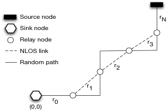
In this paper, while continuing to assume (a) that a single operative moves step-by-step along a path, deciding to place or to not place a relay, (b) that the length of the path is a geometrically distributed random multiple of the step size, (c) that a source of packets is placed at the end of the path, (d) that the lone packet traffic model applies, and (e) that the total cost of a deployment is a linear combination of the sum of convex hop costs and the number of nodes placed, we extend the work presented in [9] to the two-dimensional case. At each step, the line can take a right angle turn either to the “East” or to the “North” with known fixed probabilities. We assume a Non-Line-Of-Sight (NLOS) propagation model, where a radio link exists between two nodes placed anywhere on the path, see Fig. 2. The lone packet model is a natural first assumption, and would be useful in low-duty cycle monitoring applications. Once the network has been deployed, an analytical technique such as that presented in [10] can be used to estimate the actual packet carrying capacity of the network.

We will formally describe our system model and problem formulation in Section II. The following are our main contributions:

Figure 2: A depiction of relay deployment along a random lattice path with NLOS propagation.

• We formulate the problem as a total cost Markov decision process (MDP), and characterize the optimal policies in terms of placement sets. We show that these optimal policies are threshold policies and thus the placement sets are characterized by boundaries in the two-dimensional lattice (Section III). Beyond these boundaries, it is optimal to place a relay.

• Noticing that placement instants are renewal points in the random process, we recognize and prove the One-Step-Look-Ahead (OSLA) characterization of the placement sets (Section IV).

• Based on the OSLA characterization, we propose an iterative algorithm, which converges to the optimal placement set in a finite number of steps (Section V). We have observed that this algorithm converges much faster than value iteration.

• In Section VII we provide several numerical results that illustrate the theoretical development. The relay placement approach proposed in [4, 5, 6, 7] would suggest a distance threshold based placement rule. We numerically obtain the optimal rule in this class, and find that the cost of this policy is numerically indistinguishable from that of the overall optimal policy provided by our theoretical development. It suggests that it might suffice to utilize a distance threshold policy. However, the distance threshold should be carefully designed taking into account the system parameters and the optimality objective.

For the ease of presentation we have moved most of the proofs to the Appendix.

II System Model

We consider a deployment person, whose stride length is 1 unit, moving along a random path in the two-dimensional lattice, placing relays at some of the lattice points of the path and finally a source node at the end of the path. Once placed, the source node periodically generates measurement packets which are forwarded by the successive relays in a multihop fashion to the control centre located at $(0,0)$; see Fig. 2.

II-A Random Path

Let $\mathbb{Z}_{+}$ denote the set of nonnegative integers, and $\mathbb{Z}_{+}^{2}$ the nonnegative orthant of the two dimensional integer lattice. We will refer to the $\mathsf{x}$ direction as East and to the $\mathsf{y}$ direction as North. Starting from $(0,0)$ there is a lattice path that takes random turns to the North or to the East (this is to avoid the path folding back onto itself, see Fig 2). Under this restriction, the path evolves as a stochastic process over $\mathbb{Z}_{+}^{2}$. When the deployment person has reached some lattice point, the path continues for one more step and terminates with probability $p$, or does not terminate with probability $1-p$. In either case, the next step is Eastward with probability $q$ and Northward with probability $1-q$. Thus, for instance, $(1-p)q$ is the probability that the path proceeds Eastwards without ending. The person deploying the relays is assumed to keep a count of $m$ and $n$, the number of steps taken in the $\mathsf{x}$ direction and in $\mathsf{y}$ direction, repectively, since the previous relay was placed. He is also assumed to know the probabilities $p$ and $q$.

II-B Cost Definition

In our model, we assume NLOS propagation, i.e., packet transmission can take place between any two successive relays even if they are not on the same straight line segment of the lattice path. In the building context, this would correspond to the walls being radio transparent. The model is also suitable when the deployment region is a thickly wooded forest where the deployment person is restricted to move only along some narrow path (lattice edges in our model).

For two successive relays separated by a distance $r$, we assign a cost of $d(r)$ which could be the average delay incurred over that hop (including transmission overheads and retransmission delays), or the power required to get a packet across the hop. For instance, in our numerical work we use the power cost, $d(r)=P_{m}+\gamma r^{\eta}$, where $P_{m}$ is the minimum power required, $\gamma$ represents an SNR constraint and $\eta$ is the path-loss exponent. Now suppose $N$ relays are placed such that the successive inter-relay distances are $r_{0},r_{1},\cdots,r_{N}$ ($r_{0}$ is the distance from the control centre at $(0,0)$ and the first relay, and $r_{N}$ is the distance from the last relay to the sensor placed at the end of the path) then the total cost of this placement is the sum of the one-hop costs $C=\sum_{i=0}^{N}d(r_{i})$. The total cost being the sum of one-hop costs can be justified for the lone packet model since when a packet is being forwarded there is no other packet transmission taking place.

We now impose a few technical conditions on the one-hop cost function $d(\cdot)$: (C1) $d(0)>0$, (C2) $d(r)$ is convex and increasing in $r$, and (C3) for any $r$ and $\delta>0$ the difference $d(r+\delta)-d(r)$ increases to $\infty$.

(C1) is imposed considering the fact that it requires a non-zero amount of delay or power for transmitting a packet between two nodes, however close they may be. (C2) and (C3) are properties we require to establish our results on the optimal policies. They are satisfied by the power cost, $P_{m}+\gamma r^{\eta}$ , and also by the mean hop delay (see [11]).

We will overload the notation $d(\cdot)$ by denoting the one-hop cost between the locations $(0,0)$ and $(x,y)\in\Re^{2}$ as simply $d(x,y)$ instead of $d(||(x,y)-(0,0)||)$. Using the condition on $d(r)$ we prove the following convexity result of $d(x,y)$.

Lemma 1

The function $d(x,y)$ is convex in $(x,y)$, where $(x,y)\in\mathbb{R}^{2}$.

Proof:

This follows from the fact that $d(\cdot)$ is convex, non-decreasing in its argument. For a formal proof, see Appendix A-A. ∎

We further impose the following condition on $d(x,y)$ where $(x,y)\in\Re^{2}$. We allow a general cost-function $d(x,y)$ endowed with the following property: (C4) The function $d(x,y)$ is positive, twice continuously partially differentiable in variables $x$ and $y$ and $\forall x,y\in\mathbb{R}_{+}$,

$$d_{xx}(x,y)>0,\hskip 5.0ptd_{xy}(x,y)>0,\hskip 5.0ptd_{yy}(x,y)>0,$$ (1)

where $d_{xy}(x,y)=\frac{\partial^{2}d(x,y)}{\partial x\partial y}$. These properties also hold for the mean delay and the power functions mentioned earlier.

Finally define, for $(m,n)\in\mathbb{Z}_{+}^{2}$, $\Delta_{1}(m,n)=d(m+1,n)-d(m,n)$ and $\Delta_{2}(m,n)=d(m,n+1)-d(m,n)$.

Lemma 2

$\Delta_{1}(m,n)$ and $\Delta_{2}(m,n)$ are non-decreasing in both the coordinates $m$ and $n$.

Proof:

This follows directly from (1). See Appendix A-B for details. ∎

II-C Deployment Policies and Problem Formulation

A deployment policy $\pi$ is a sequence of mappings $(\mu_{k}:k\geq 0)$, where at the $k$-th step of the path (provided that the path has not ended thus far) $\mu_{k}$ allows the deployment person to decide whether to place or not to place a relay where, in general, randomization over these two actions is allowed. The decision is based on the entire information available to the deployment person at the $k$-th step, namely the set of vertices traced by the path and the location of the previous vertices where relays were placed. Let $\Pi$ represent the set of all policies. For a given policy $\pi\in\Pi$, let $\mathbb{E}_{\pi}$ represent the expectation operator under policy $\pi$. Let $C$ denote the total cost incurred and $N$ the total number of relays used. We are interested in solving the following problem,

$$\min_{\pi\in\Pi} \mathbb{E}_{\pi}C+\lambda\mathbb{E}_{\pi}N,$$ (2)

where $\lambda>0$ may be interpreted as the cost of a relay. Solving the problem in (2) can also help us solve the following constrained problem,

$$\min_{\pi\in\Pi} \mathbb{E}_{\pi}C$$

Subject to: $$\mathbb{E}_{\pi}N\leq\rho_{avg},$$ (3)

where $\rho_{avg}>0$ is a contraint on the average number of relays (we will describe this procedure in Section VI). First, in Sections III to V, we work towards obtaining an efficient solution to the problem in (2).

III MDP Formulation and Solution

In this section we formulate the problem in (2) as a total cost infinite horizon MDP and derive the optimal policy in terms of optimal placement set. We show that this set is characterized by a two-dimensional boundary, upon crossing which it is optimal to place a relay.

III-A States, Actions, State-Transitions and Cost Structure

We formulate the problem as a sequential decision process starting at the origin of the lattice path. The decision to place or not place a relay at the $k$-th step is based on $((M_{k},N_{k}),Z_{k})$, where $(M_{k},N_{k})$ denotes the coordinates of the deployment person with respect to the previous relay and $Z_{k}\in\{\mathsf{e},\mathsf{c}\}$; $Z_{k}=\mathsf{e}$ means that at step $k$ the random lattice path has ended and $Z_{k}=\mathsf{c}$ means that the path will continue in the same direction for at least one more step. Thus, the state space is given by:

$$\mathcal{S}=\Big{\{}(m,n,z):(m,n)\in\mathbb{Z}_{+}^{2},z\in\{\mathsf{e},\mathsf{c}\}\Big{\}}\cup\{\phi\},$$ (4)

where $\phi$ denotes the cost-free terminal state, i.e., the state after the end of the path has been discovered. The action taken at step $k$ is denoted $U_{k}\in\{0,1\}$, where $U_{k}=1$ is the action to place a relay, and $U_{k}=0$ is the action of not placing a relay. When the state is $(m,n,\mathsf{c})$ and when action $u$ is taken, the transition probabilities are given by:

• If $u$ is $0$ then,
  (i) $(m,n,\mathsf{c})$ $\longrightarrow$ $(m+1,n,\mathsf{c})$ w.p. $(1-p)q$
  (ii) $(m,n,\mathsf{c})$ $\longrightarrow$ $(m+1,n,\mathsf{e})$ w.p. $pq$
  (iii) $(m,n,\mathsf{c})$ $\longrightarrow$ $(m,n+1,\mathsf{c})$ w.p. $(1-p)(1-q)$
  (iv) $(m,n,\mathsf{c})$ $\longrightarrow$ $(m,n+1,\mathsf{e})$ w.p. $p(1-q)$.

• If $u$ is $1$ then
  (i) $(m,n,\mathsf{c})\longrightarrow(1,0,\mathsf{c})$ w.p.  $(1-p)q$
  (ii) $(m,n,\mathsf{c})\longrightarrow(1,0,\mathsf{e})$ w.p.  $pq$
  (iii) $(m,n,\mathsf{c})\longrightarrow(0,1,\mathsf{c})$ w.p.  $(1-p)(1-q)$
  (iv) $(m,n,\mathsf{c})\longrightarrow(0,1,\mathsf{e})$ w.p.  $p(1-q)$.

If $Z_{k}=\mathsf{e}$ then the only allowable action is $u=1$ and we enter into the state $\phi$. If the current state is $\phi$, we stay in the same cost-free termination state irrespective of the control $u$. The one step cost when the state is $s\in\mathcal{S}$ is given by:

$$c(s,u)=\left\{\begin{array}[]{l l}d(m,n)&\mbox{ if }s=(m,n,\mathsf{e}),\\ \lambda+d(m,n)&\mbox{ if }u=1\mbox{ and }s=(m,n,\mathsf{c}),\\ 0&\mbox{ if }u=0\mbox{ or }s=\phi.\end{array}\right.$$

For simplicity we write the state $(m,n,\mathsf{c})$ as simply $(m,n)$.

III-B Optimal Placement Set $\mathcal{P}_{\lambda}$

Let $J_{\lambda}(m,n)$ denote the optimal cost-to-go when the current state is $(m,n)$. When at some step the state is $(m,n)$ the deployment person has to decide whether to place or not place a relay at the current step. $J_{\lambda}$ is the solution of the Bellman equation [12, Page 137, Prop. 1.1],

$$J_{\lambda}(m,n)=\min\{c_{p}(m,n),c_{np}(m,n)\},$$ (6)

where $c_{p}(m,n)$ and $c_{np}(m,n)$ denote the expected cost incurred when the decision is to place and not place a relay, respectively. $c_{p}(m,n)$ is given by

$$c_{p}(m,n) = \lambda+d(m,n)+(1-p)(1-q)J_{\lambda}(0,1)$$ (7)

$$+(1-p)qJ_{\lambda}(1,0)+pd(1).$$

The term $\lambda+d(m,n)$ in the above expression is the one step cost which is first incurred when a relay is placed. The remaining terms are the average cost-to-go from the next step. The term $(1-p)(1-q)J_{\lambda}(0,1)$ can be understood as follows: $(1-p)(1-q)$ is the probability that the path proceeds Eastward without ending. Thus the state at the next step is $(0,1,\mathsf{c})$ w.p. $(1-p)(1-q)$, the optimal cost-to-go from which is, $J_{\lambda}(0,1)$. Similarly for the term $(1-p)qJ_{\lambda}(1,0)$, $(1-p)q$ is the probability that the path will proceed, without ending, towards the North (thus the next state is $(1,0,\mathsf{c})$) and $J_{\lambda}(1,0)$ is the cost-to-go from the next state. Finally, in the term $pd(1)$, $p$ is the probability that the path will end, either proceeding East or North, at the next step and $d(1)$ is the cost of the last link. Following a similar explanation, the expression for $c_{np}(m,n)$ can be written as:

$$c_{np}(m,n)=$$ (8)

$$(1-p)qJ_{\lambda}(m+1,n)+(1-p)(1-q)J_{\lambda}(m,n+1)$$

$$+pqd(m+1,n)+p(1-q)d(m,n+1).$$

We define the optimal placement set $\mathcal{P}_{\lambda}$ as the set of all lattice points $(m,n)$, where it is optimal to place rather than to not place a relay. Formally,

$$\mathcal{P}_{\lambda}=\Big{\{}(m,n):c_{p}(m,n)\leq c_{np}(m,n)\Big{\}}.$$ (9)

In this definition, if the costs of placing and not-placing are the same, we have arbitrarily chosen to place at that point.

The above result yields the following main theorem of this section which characterizes the optimal placement set $\mathcal{P}_{\lambda}$ in terms of a boundary.

Theorem 1

The optimal placement set $\mathcal{P}_{\lambda}$ is characterized by a boundary, i.e., there exist mappings $m^{*}:\mathbb{Z}_{+}\rightarrow\mathbb{Z}_{+}$ and $n^{*}:\mathbb{Z}_{+}\rightarrow\mathbb{Z}_{+}$ such that:

$$\mathcal{P}_{\lambda} = \bigcup_{n\in\mathbb{Z}_{+}}\{(m,n):m\geq m^{*}(n)\}$$ (10)

$$= \bigcup_{m\in\mathbb{Z}_{+}}\{(m,n):n\geq n^{*}(m)\}.$$ (11)

Proof:

The proof utilizes the conditions C2 and C3 imposed on the cost function $d(\cdot)$. First, using (7) and (8) in (9) and rearranging we alternatively write $\mathcal{P}_{\lambda}$ as, $\mathcal{P}_{\lambda}=\{(m,n):F(m,n)\geq K\}$, where $K$ is a constant and $F(\cdot,\cdot)$ is some function of $m$ and $n$. Then, we complete the proof by showing that $F(m,n)$ is non-decreasing in both $m$ and $n$. This requires us to prove (using an induction argument) that $H_{\lambda}(m,n):=J_{\lambda}(m,n)-d(m,n)$ is non-decreasing in $m$ and $n$. Also, Lemma 2 has to be used here. For a formal proof see Appendix B. ∎

Remark: Though the optimal placement set $\mathcal{P}_{\lambda}$ was characterized nicely in terms of a boundary $m^{*}(\cdot)$ and $n^{*}(\cdot)$, a naive approach of computing this boundary, using value iteration to obtain $J_{\lambda}(m,n)$ (for several values of $(m,n)\in\mathbb{Z}_{+}^{2}$), would be computationally intensive. Our effort in the next section (Section IV) is towards obtaining an alternate simplified representation for $\mathcal{P}_{\lambda}$ using which we propose an algorithm in Section V, which is guaranteed to return $\mathcal{P}_{\lambda}$ in a finite (in practice, small) number of steps.

IV Optimal Stopping Formulation

We observe that the points where the path has not ended, and a relay is placed, are renewal points of the decision process. This motivates us to think of the decision process after a relay is placed as an optimal stopping problem with termination cost $J_{\lambda}(0,0)$ (which is the optimal cost-to-go from a relay placement point). Let $\overline{\mathcal{P}}_{\lambda}$ denote the placement set corresponding to the OSLA rule (to be defined next). In this section we prove our next main result that $\mathcal{P}_{\lambda}=\overline{\mathcal{P}}_{\lambda}$.

IV-A One-Step-Look-Ahead Stopping Set $\overline{\mathcal{P}}_{\lambda}$

Under the OSLA rule, a relay is placed at state $(m,n,\mathsf{c})$ if and only if the “cost $c_{1}(m,n)$ of stopping (i.e., placing a relay) at the current step” is less than the “cost $c_{2}(m,n)$ of continuing (without placing relay at the current step) for one more step, and then stopping (i.e., placing a relay at the next step)”. The expressions for the costs $c_{1}(m,n)$ and $c_{2}(m,n)$ can be written as:

$$c_{1}(m,n) = \lambda+d(m,n)+J_{\lambda}(0,0)$$

and

$$c_{2}(m,n)=$$

$$pq(d(m+1,n)+p(1-q)d(m,n+1))+(1-p)$$

$$\Big{(}qd(m+1,n)+(1-q)d(m,n+1)+\lambda+J_{\lambda}(0,0)\Big{)}.$$

Then we define the OSLA placement set $\overline{\mathcal{P}}_{\lambda}$ as:

$$\overline{\mathcal{P}}_{\lambda} = \{(m,n)\in\mathbb{Z}_{+}^{2}:c_{1}(m,n)\leq c_{2}(m,n)\}.$$

Substituting for $c_{1}(m,n)$ and $c_{2}(m,n)$ and simplifying we obtain:

$$\overline{\mathcal{P}}_{\lambda}=\Big{\{}(m,n)\in\mathbb{Z}_{+}^{2}:p(\lambda+J_{\lambda}(0,0))\leq\Delta_{q}(m,n)\Big{\}},$$ (12)

where $\Delta_{q}(m,n)=q\Delta_{1}(m,n)+(1-q)\Delta_{2}(m,n)$.

Theorem 2

The OSLA rule is a threshold policy, i.e., there exist mappings $\bar{m}:\mathbb{Z}_{+}\rightarrow\mathbb{Z}_{+}$ and $\bar{n}:\mathbb{Z}_{+}\rightarrow\mathbb{Z}_{+}$, which define the one-step placement set $\overline{\mathcal{P}}_{\lambda}$ as follows,

$$\overline{\mathcal{P}}_{\lambda} = \bigcup_{n\in\mathbb{Z}_{+}}\{(m,n):m\geq\bar{m}(n)\}$$ (13)

$$= \bigcup_{m\in\mathbb{Z}_{+}}\{(m,n):n\geq\bar{n}(m)\}.$$ (14)

Proof:

Noticing that in (12) $\Delta_{q}(m,n)$ is non-decreasing in $(m,n)$ and $p(\lambda+J_{\lambda}(0,0))$ is a constant, the proof follows along the lines of the proof of Theorem 1. ∎

Now, we present the main theorem of this section.

Theorem 3

$$\mathcal{P}_{\lambda}=\overline{\mathcal{P}}_{\lambda}.$$

Proof:

See Appendix C. ∎

Remark: The characterization in (12) is much simpler than the one in (B) once the value of $J_{\lambda}(0,0)$ is given. In the following subsection, we define a function $g(\cdot)$ and express $J_{\lambda}(0,0)$ as the minimum value of this function.

IV-B Computation of $J_{\lambda}(0,0)$

Let us start by defining a collection of placement sets indexed by $h\geq 0$:

$${\mathcal{P}}(h)=\{(m,n)\in\mathbb{Z}_{+}^{2}:p(\lambda+h)\leq\Delta_{q}(m,n)\}.$$ (15)

Referring to (12), note that ${\mathcal{P}}(J_{\lambda}(0,0))=\overline{\mathcal{P}}_{\lambda}$. Let $g(h)$ denote the cost-to-go, starting from $(0,0)$, if the placement set $\mathcal{P}(h)$ is employed. Then, since $J_{\lambda}(0,0)$ is the optimal cost-to-go and $\mathcal{P}_{\lambda}\in\{{\mathcal{P}}(h)\}_{h\geq 0}$, we have $J_{\lambda}(0,0)=\min_{h\geq 0}g(h)$.

To compute $g(h)$, we proceed by defining the boundary $\mathcal{B}(h)$ of $\mathcal{P}(h)$ as follows:

$$\mathcal{B}(h) = \{(m,n)\in\mathcal{P}(h):(m-1,n)\in\mathcal{P}^{c}(h)\mbox{ or }$$ (16)

$$\hskip 11.38109pt(m,n-1)\in\mathcal{P}^{c}(h)\},$$

where $\mathcal{P}^{c}(h):=\mathbb{Z}_{+}^{2}-\mathcal{P}(h)$.

Suppose the corridor ends at some $(m,n)\in\mathcal{P}^{c}(h)\cup\mathcal{B}(h)$, then only a cost of $d(m,n)$ is incurred. Otherwise (i.e., if the corridor reaches some $(m,n)\in\mathcal{B}(h)$ and continues), using a renewal argument, a cost of $d(m,n)+\lambda+g(h)$ is incurred, where $d(m,n)+\lambda$ is the cost of placing a relay and $g(h)$ is the future cost-to-go. We can thus write:

$$g(h) = \sum_{(m,n)\in\mathcal{P}^{c}(h)\cup\mathcal{B}(h)}\mathbb{P}((m,n),\mathsf{e})d(m,n)+$$ (17)

$$\sum_{(m,n)\in\mathcal{B}(h)}\!\mathbb{P}((m,n),\mathsf{c})(g(h)\!+\!\lambda\!+\!d(m,n)),\;\;\;$$

where $\mathbb{P}((m,n),\mathsf{e})$ is the probability of the corridor ending at $(m,n)$ and $\mathbb{P}((m,n),\mathsf{c})$ is the probability of the corridor reaching the boundary and continuing. Solving for $g(h)$, we obtain:

$$g(h) = \frac{1}{1-\sum_{(m,n)\in\mathcal{B}(h)}\mathbb{P}((m,n),\mathsf{c})}\times$$ (18)

$$\Bigg{(}\sum_{(m,n)\in\mathcal{P}^{c}(h)\cup\mathcal{B}(h)}\mathbb{P}((m,n),\mathsf{e})d(m,n)+$$

$$\sum_{(m,n)\in\mathcal{B}(h)}\mathbb{P}((m,n),\mathsf{c})(\lambda+d(m,n))\Bigg{)}.$$

The above expression is extensively used in our algorithm proposed in the next section.

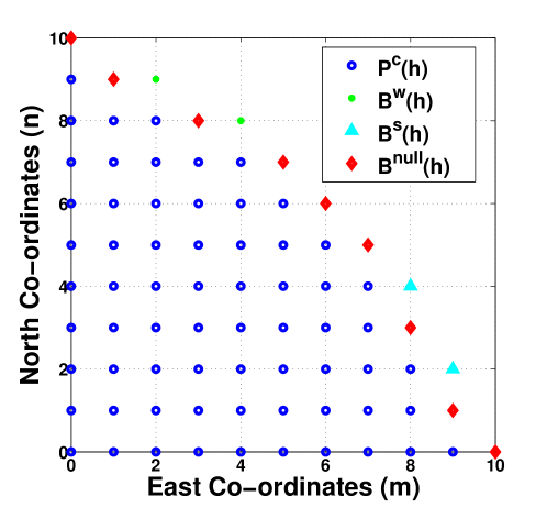
We conclude this subsection by deriving the expression for the probabilities $\mathbb{P}((m,n),\mathsf{e})$ and $\mathbb{P}((m,n),\mathsf{c})$. Let us partition the boundary $\mathcal{B}(h)$ into three mutually disjoint sets:

$$\mathcal{B}^{w}(h) = \{(m,n)\in\mathcal{B}(h):(m-1,n)\in\mathcal{B}(h)\}$$

$$\mathcal{B}^{s}(h) = \{(m,n)\in\mathcal{B}(h):(m,n-1)\in\mathcal{B}(h)\}$$

$$\mathcal{B}^{null}(h) = \{(m,n)\in\mathcal{B}(h):(m-1,n)\notin\mathcal{B}(h)\mbox{ and }$$

$$(m,n-1)\notin\mathcal{B}(h)\}.$$

For a depiction of the various boundary points, see Fig. 3.

Figure 3: Example of placement set of the form in (15): ’o’ denotes lattice points outside the placement set; lattice points on the boundary can be partitioned into three sets according to the direction, from which they can be reached.

Now, $\mathbb{P}((m,n),\mathsf{e})$ can be written as:

$$\mathbb{P}((m,n),\mathsf{e})=$$

$$\left\{\begin{array}[]{lr}\binom{m+n}{m}p(1-p)^{m+n-1}q^{m}(1-q)^{n}\\ \hskip 85.35826pt\mbox{ if }(m,n)\in\mathcal{P}^{c}(h)\cup\mathcal{B}^{null}(h)\\ \binom{m+n-1}{m}p(1\!-\!p)^{m+n-1}q^{m}(1\!-\!q)^{n}\mbox{ if }(m,n)\!\in\!\mathcal{B}^{w}(h)\\ \binom{m+n-1}{m-1}p(1\!-\!p)^{m+n-1}q^{m}(1\!-\!q)^{n}\mbox{ if }(m,n)\!\in\!\mathcal{B}^{s}(h).\end{array}\right.$$

This can be understood as follows. Any point $(m,n)\in\mathcal{P}^{c}(h)\cup\mathcal{B}^{null}(h)$ can be reached from West or South. $\binom{m+n}{m}$ is the number of possible paths for reaching $(m,n)$. Each such path has to go $m$ times Eastwards (thus the term $q^{m}$) and $n$ times Northwards (thus the term $(1-q)^{n}$) and finally ending at $(m,n)$ (thus the term $p(1-p)^{m+n-1}$). Any point $(m,n)\in\mathcal{B}^{w}(h)$ can be reached only from South point $(m,n-1)$. The probability of reaching $(m,n-1)$ without ending is $\binom{m+n-1}{m}(1-p)^{m+n-1}q^{m}(1-q)^{n-1}$. Then, the corridor reaches $(m,n)$ and ends with probability $p(1-q)$. $\mathbb{P}((m,n),\mathsf{e})$ for $(m,n)\in\mathcal{B}^{s}(h)$ can be obtained analogously.

Similarly, $\mathbb{P}((m,n),\mathsf{c})$ can be written as:

$$\mathbb{P}((m,n),\mathsf{c})=$$

$$\left\{\begin{array}[]{ll}\binom{m+n}{m}(1-p)^{m+n}q^{m}(1-q)^{n}\\ \hskip 85.35826pt\mbox{ if }(m,n)\in\mathcal{P}^{c}(h)\cup\mathcal{B}^{null}(h)\\ \binom{m+n-1}{m}(1-p)^{m+n}q^{m}(1-q)^{n}\mbox{ if }(m,n)\in\mathcal{B}^{w}(h)\\ \binom{m+n-1}{m-1}(1-p)^{m+n}q^{m}(1-q)^{n}\mbox{ if }(m,n)\in\mathcal{B}^{s}(h).\end{array}\right.$$

V OSLA Based Fixed Point Iteration Algorithm

In this section, we present an efficient fixed point iteration algorithm (Algorithm 1) using the OSLA rule in (12) for obtaining the optimal placement set, $\mathcal{P}_{\lambda}$, and the optimal cost-to-go, $J_{\lambda}(0,0)$. There are two advantages of our algorithm over the naive approach of directly trying to minimize the function $g(\cdot)$ to obtain $J_{\lambda}(0,0)$ (recall that $J_{\lambda}(0,0)=\min_{h\geq 0}g(h)$):

• On the theoretical side, this iterative algorithm avoids explicit optimization altogether, which, otherwise would be performed numerically over a continuous range. Without any structure on the objective function, direct numerical minimization of $g(\cdot)$ is difficult and often unsatisfactory, as it invariably uses some sort of heuristic search over this continuous range.

• On the practical side, this algorithm is proved to converge within a finite number of iterations and observed to be extremely fast (requires 3 to 4 iterations typically).

The following is our Algorithm which we refer to as the OSLA Based Fixed Point Iteration Algorithm.

Algorithm 1 OSLA Based Fixed Point Iteration Algorithm

0:  $0<p<1$, $0\leq q\leq 1$, $\lambda\geq 0$

1:  $k=0$, $h^{(k)}=0$

2:  while 1 do

3:     $\mathcal{P}(h^{(k)})\leftarrow\{(m,n)\in\mathbb{Z}_{+}^{2}:p(\lambda+h^{(k)})\leq\Delta_{q}(m,n)\}$

4:     Compute $g(h^{(k)})$ using (18)

5:     if $g(h^{(k)})==h^{(k)}$ then

6:        Break;

7:     end if

8:     $h^{(k+1)}\leftarrow g(h^{(k)})$

9:     $k\leftarrow k+1$

10:  end while

11:  return $g(h^{(k)})$, $\mathcal{P}(h^{(k)})$

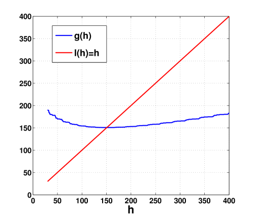
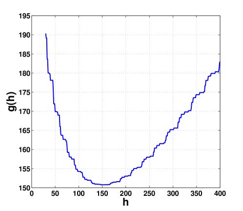
We now prove the correctness and finite termination properties of our algorithm. First, we define $g^{*}:=J_{\lambda}(0,0)=\min_{h\geq 0}g(h)$. Now consider a sample plot of the function $g(h)$ in Fig. 4. From Fig. 4 observe that whenever $h>g^{*}$ (which is around 150), $h>g(h)$. Also, Fig. 4 (where we have plotted the functions $g(h)$ and $l(h)=h$) suggests that $g(h)$ has a unique fixed point. We formally prove these results.

Figure 4: 4 Cost-to-go $g(h)$ as a function of $h$ 4 Zoom on the cost-to-go $g(h)$ as a function of $h$. These plots are for $p=0.02$, $q=0.5$, and $\lambda=41$.

Lemma 3

If $h>g^{*}$ then $h>g(h)$.

Proof:

This follows from the manipulation of (18). See Appendix D for details. ∎

Lemma 4

$g(h)$ has a unique fixed point.

Proof:

From (15) and (12), we observe that $\mathcal{P}(J_{\lambda}(0,0))=\overline{\mathcal{P}}_{\lambda}$. From Theorem 3, $\overline{\mathcal{P}}_{\lambda}$ is the optimal placement set and thus the cost-to-go of using $\mathcal{P}(J_{\lambda}(0,0))$ is $J_{\lambda}(0,0)$, i.e., $g(J_{\lambda}(0,0))=J_{\lambda}(0,0)$. Hence, $J_{\lambda}(0,0)=g^{*}$ is a fixed point of $g(\cdot)$. Now, any $h>g^{*}$ cannot be a fixed point since, in this case, $h>g(h)$ from Lemma 3. On the other hand, any $h<g^{*}$ is such that $h<g^{*}\leq g(h)$ because $g^{*}$ is the optimal cost-to-go. Hence, $g^{*}$ is the unique fixed point of $g(\cdot)$. ∎

We are now ready to prove the convergence property of our Algorithm.

Lemma 5

1. The sequence $\{h^{(k)}\}_{k\geq 1}$ (in Algorithm 1) is non-increasing, i.e., $h^{(k+1)}\leq h^{(k)}$, with the equality sign holding if and only if $h^{(k)}=g^{*}$.

2. The sequence ${\{\mathcal{P}^{c}(h^{(k)})}\}_{k\geq 1}$ is non-increasing, i.e., $\mathcal{P}^{c}(h^{(k+1)})\subseteq\mathcal{P}^{c}(h^{(k)})$, where the containment is strict whenever $\mathcal{P}^{c}(h^{(k+1)})\varsubsetneq{\mathcal{P}_{\lambda}}^{c}$.

Proof:

1) Note first that $h^{(k)}\geq g^{*}$ for $k\geq 1$ because $h^{(k)}=g(h^{(k-1)})\geq g^{*}$. Then, for $k\geq 1$, we have either $h^{(k)}=g^{*}$ or $h^{(k)}>g^{*}$. In the first case $h^{(k+1)}=g(h^{(k)})=g(g^{*})=g^{*}=h^{(k)}$ and we can stop, whereas in the second case, from Lemma 3 we have $h^{(k+1)}=g(h^{(k)})<h^{(k)}$.

2) From (15), $h_{2}>h_{1}$ implies $\mathcal{P}^{c}(h_{1})\subseteq\mathcal{P}^{c}(h_{2})$. Hence, as $\{h^{(k)}\}_{k\geq 1}$ is non-increasing (from Part 1)), ${\{\mathcal{P}^{c}(h^{(k)})}\}_{k\geq 1}$ is also non-increasing.

Suppose $\mathcal{P}^{c}(h^{(k+1)})=\mathcal{P}^{c}(h^{(k)})$ then $g(h^{(k+1)})=g(h^{(k)})=h^{(k+1)}$ (second equality is by the definition of $\{h^{(k)}\}$), which implies $h^{(k+1)}=g^{*}$ (since $g(\cdot)$ has a unique fixed point, see Lemma 4). Thus, $\mathcal{P}^{c}(h^{(k+1)})={\mathcal{P}_{\lambda}}^{c}$. ∎

Theorem 4

Algorithm 1 returns $g^{*}$ and ${\mathcal{P}_{\lambda}}^{c}$ in a finite number of steps.

Proof:

Noting that $h^{(1)}=g(h^{(0)})\geq g^{*}$ and using (15), we have ${\mathcal{P}_{\lambda}}^{c}\subseteq\mathcal{P}^{c}(h^{(1)})$. Either ${\mathcal{P}_{\lambda}}^{c}=\mathcal{P}^{c}(h^{(1)})$, in which case the algorithm stops. Otherwise, note that both sets, ${\mathcal{P}_{\lambda}}^{c}$ and $\mathcal{P}^{c}(h^{(1)})$ contain a finite number of lattice points (from the definition of $\mathcal{P}(h)$ in (15)). Using Lemma 5, $\mathcal{P}^{c}(h^{(k)})$ converges to ${\mathcal{P}_{\lambda}}^{c}$ in at most $|\mathcal{P}^{c}(h^{(1)})-{\mathcal{P}_{\lambda}}^{c}|<\infty$ iterations. Once $\mathcal{P}^{c}(h^{(k)})$ converges to ${\mathcal{P}_{\lambda}}$, the algorithm stops and returns the optimal cost-to-go $g^{*}$. ∎

VI Solving the Constrained Problem

In this section, we devise a method to solve the constrained problem in (II-C) using the solution of the unconstrained problem (2) provided by Algorithm 1. This method is applied in Section VII-B where, imposing a constraint on the average number of relays, we compare the performance of a distance based heuristic with the optimal.

We begin with the following standard result which relates the solutions of the problems in (2) and (II-C).

Lemma 6

Let $\pi_{\lambda}^{*}\in\Pi$ be an optimal policy for the unconstrained problem in (2) such that $\mathbb{E}_{\pi_{\lambda}^{*}}N=\rho_{avg}$. Then $\pi_{\lambda}^{*}$ is also optimal for the constrained problem in (II-C).

However, the above lemma is useful only when we are able to exhibit a $\lambda$ such that $\mathbb{E}_{\pi_{\lambda}^{*}}N=\rho_{avg}$. The subsequent development in this section is towards obtaining the solution to the more general case.

The expected number of relays used by the optimal policy, $\pi_{\lambda}^{*}$, which uses the optimal placement set $\mathcal{P}_{\lambda}$, can be computed as:

$$\mathbb{E}_{\pi_{\lambda}^{*}}N=\frac{\sum_{(m,n)\in\mathcal{B}_{\lambda}}\mathbb{P}((m,n),\mathsf{c})}{1-\sum_{(m,n)\in\mathcal{B}_{\lambda}}\mathbb{P}((m,n),\mathsf{c})},$$ (21)

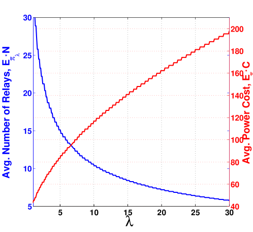
where $\mathbb{P}((m,n),\mathsf{c})$ is the reaching probability corresponding to $\mathcal{P}_{\lambda}$ and $\mathcal{B}_{\lambda}$ is the boundary of $\mathcal{P}_{\lambda}$. A plot of $\mathbb{E}_{\pi_{\lambda}^{*}}N$ vs. $\lambda$ is given in Fig. 5. We make the following observations about $\mathbb{E}_{\pi_{\lambda}^{*}}N$.

1) $\mathbb{E}_{\pi_{\lambda}^{*}}N$ decreases with $\lambda$; this is as expected, since as each relay becomes “costlier” fewer relays are used on the average.

2) Even when $\lambda=0$, $\mathbb{E}_{\pi_{\lambda}^{*}}N$ is finite. This is because $d(0)>0$, i.e., there is a positive cost for a $0$ length link. Define the value of $\mathbb{E}_{\pi_{\lambda}^{*}}N$ with $\lambda=0$ to be $\rho_{\max}$.

3) $\mathbb{E}_{\pi_{\lambda}^{*}}N$ vs. $\lambda$ is a piecewise constant function. This occurs because the relay placement positions are discrete. For a range of values of $\lambda$ the same threshold is optimal. This structure is also evident from the results based on the optimal stopping formulation and the OSLA rule in Section IV. It follows that for a value of $\lambda$ at which there is a step in the plot, there are two optimal deterministic policies, $\underline{\pi}$ and $\overline{\pi}$, for the relaxed problem. Let $\underline{\rho}=\mathbb{E}_{\underline{\pi}}N$ and $\overline{\rho}=\mathbb{E}_{\overline{\pi}}N$.

We have the following structure of the optimal policy for the constrained problem:

Theorem 5

1. For $\rho_{avg}\geq\rho_{max}$ the optimal placement set is obtained for $\lambda=0$, i.e., is $\mathcal{P}_{0}$.

2. For $\rho_{avg}<\rho_{max}$, if there is a $\lambda$ such that (a) $\mathbb{E}_{\pi_{\lambda}^{*}}N=\rho_{avg}$ then the optimal policy is $\pi_{\lambda}^{*}$, or (b) $\underline{\rho}<\rho_{avg}<\overline{\rho}$ then the optimal policy is obtained by mixing $\underline{\pi}$ and $\overline{\pi}$.

Proof:

1) is straight forward. For proof of 2)-(a), see Lemma 6. Considering now 2)-(b), define $0<\alpha<1$ such that $(1-\alpha)\underline{\rho}+\alpha\bar{\rho}=\rho_{avg}$. We obtain a mixing policy $\pi_{m}$ by choosing $\underline{\pi}$ w.p. $1-\alpha$ and $\bar{\pi}$ w.p. $\alpha$ at the beginning of the deployment. For any policy $\pi$ we have the following standard argument:

$$\mathbb{E}_{\pi_{m}}C+\lambda\mathbb{E}_{\pi_{m}}N$$ (22)

$$= (1-\alpha)(\mathbb{E}_{\underline{\pi}}C+\lambda\underline{\rho})+\alpha(\mathbb{E}_{\bar{\pi}}C+\lambda\bar{\rho})$$

$$\leq (1-\alpha)(\mathbb{E}_{\pi}C+\lambda\mathbb{E}_{\pi}N)+\alpha(\mathbb{E}_{{\pi}}C+\lambda\mathbb{E}_{\pi}N)$$

$$= \mathbb{E}_{{\pi}}C+\lambda\mathbb{E}_{\pi}N.$$

The inequality is because $\underline{\pi}$ and $\overline{\pi}$ are both optimal for the problem (2) with relay price $\lambda$. Thus, we have shown that $\pi_{m}$ is also optimal for the relaxed problem. Using this along with $\mathbb{E}_{\pi_{m}}N=\rho_{avg}$ in Lemma 6, we conclude the proof. ∎

VII Numerical Work

For our numerical work we use the one-hop power function $d(r)=P_{m}+\gamma r^{\eta}$, with $P_{m}=0.1$, $\gamma=0.01$. We first study the effect of parameter variation on the various costs. Next, we compare the performance of a distance based heuristic with the optimal.

Figure 5: Average number of relays $\mathbb{E}_{\pi_{\lambda}^{*}}N$ (left) and average power cost $\mathbb{E}_{\pi_{\lambda}^{*}}C$ (right) as a function of $\lambda$ ($p=0.002$, $q=0.5$ and $\eta=2$).

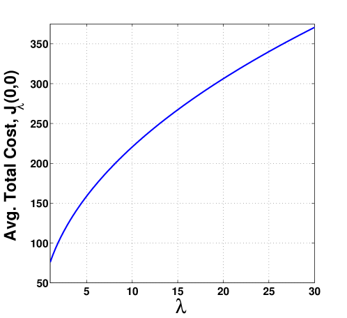
Figure 6: Average total cost $J_{\lambda}(0,0)$ as a function of $\lambda$ ($p=0.002$, $q=0.5$ and $\eta=2$).

VII-A Effect of Parameter Variation

In Fig. 3, we have already shown an optimal placement boundary for $p=0.002$, $q=0.5$, and $\eta=3$. Since $q=0.5$ the boundary is symmetric about the $m=n$ line.

In Fig. 5, we plot $E_{\pi_{\lambda}^{*}}N$ and $E_{\pi_{\lambda}^{*}}C$ vs. $\lambda$. The plot of $J_{\lambda}(0,0)$ vs. $\lambda$ is in Fig. 6. These plots are for $p=0.002$ and $q=0.5$. Since $\lambda$ is the cost per relay, as expected, $E_{\pi_{\lambda}^{*}}N$ decreases as $\lambda$ increases. We observe that $E_{\pi_{\lambda}^{*}}C$ and the optimal total cost $J_{\lambda}(0,0)$ increase as $\lambda$ increases. A close examination of Fig. 5 reveals that both the plots are step functions. This is due to the discrete placement at lattice points, which results in the same placement boundary being optimal for a range of $\lambda$ values. Thus, as seen in Section VI, at the $\lambda$ values, where there is jump in $E_{\pi_{\lambda}^{*}}N$, a random mixture of two policies is needed.

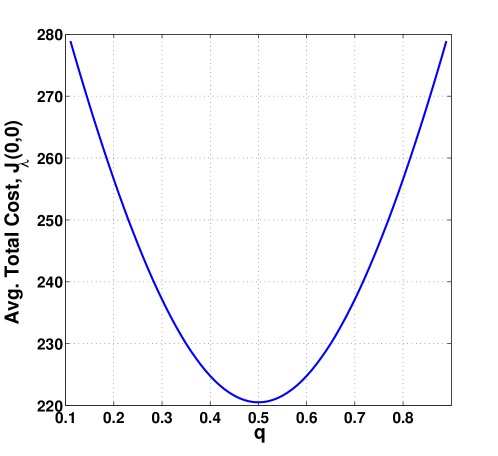
Fig. 7 shows the variation of the total optimal cost $J_{\lambda}(0,0)$ with $q$. The variation is symmetric about $q=0.5$. For a given probability $p$ of the path ending, $q=0.5$ results in the path folding frequently. In such a case, since NLOS propagation is permitted, and the path-loss is isotropic, fewer relays are required to be placed. On the other hand, when $q$ is close to $0$ or to $1$ the path takes fewer turns and more relays are needed, leading to larger values of the total cost.

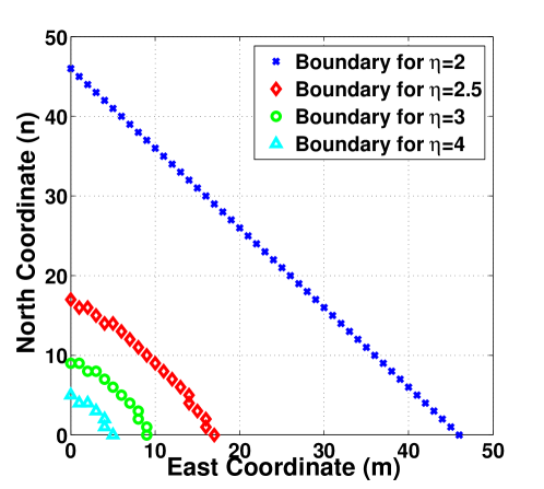
In Fig. 8 we show the variation of optimal boundaries with $\eta$. As $\eta,$ the path-loss exponent, increases the hop cost increases for a given hop distance. This results in relays needing to be placed more frequently. As can be seen the placement boundaries shrink with increasing $\eta$. We also notice that the placement boundary for $\eta=2$ is a straight line; indeed this provable result holds for $\eta=2$ for any values of $p$ and $q$.

Figure 7: Average total cost $J_{\lambda}(0,0)$ as a function of $q$ ($p=0.002$ and $\eta=2$).

Figure 8: Boundaries for various values of the path-loss exponent $\eta$ ($p=0.002$, $q=0.5$).

VII-B Comparison with the Distance based Heuristic

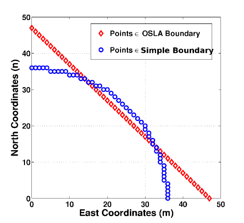
We recall from the literature survey in Section I that prior work invariably proposed the policy of placing a relay after the RF signal strength from the previous relay dropped below a threshold. For isotropic propagation (as we have assumed in this paper), this is equivalent to placing the relay after a circular boundary is crossed. With this in mind, we obtained the optimal constant distance placement policy (called the heuristic hereafter) numerically in a manner similar to what is described in Section IV-B. A sample result is provided in Fig. 9, for the parameters $p=0.002$, $q=0.5$ and $\eta=2$. We observe that if the path were to evolve roughly Eastward or Northward then the heuristic will result in many more relays being placed. On the other hand, if the path evolves diagonally (which has higher probability) then the two placement boundaries will result in similar placement decisions.

Figure 9: Boundary of the optimal placement set (OSLA boundary) and boundary derived from the heuristic policy ($p=0.002$, $q=0.5$ and $\eta=2$).

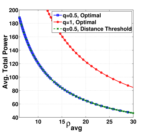
Figure 10: Average total power as a function of $\rho$ for the optimal policy ($q=0.5$ and $q=1$, which corresponds to the straight line) and for the heuristic ($q=0.5$) for $p=0.002$ and $\eta=2$.

This observation shows up in Fig. 10, where we show the cost incurred by the optimal policy (for $q=0.5$ and for $q=1$, which corresponds to a straight line corridor) and the heuristic ($q=0.5$) vs. $\rho$ for the constrained problem. As expected, the cost is much larger for $q=1$ since the path does not fold. We find that for $q=0.5$ the optimal placement boundary and the heuristic provide costs that are almost indistinguishable at this scale. We have performed simulations by varying the system parameters and observed the same good performance of the optimal constant distance placement policy. This suggests that the heuristic policy performs well provided that the threshold distance is optimally chosen with respect to the system parameters.

VIII Conclusion

We considered the problem of placing relays on a random lattice path to optimize a linear combination of average power cost and average number of relays deployed. The optimal placement policy was proved to be of threshold nature (Theorem 1). We further proved the optimality of the OSLA rule (in Theorem 3). We have also devised an OLSA based fixed point iteration algorithm (Algorithm 1), which we have proved to converge to the optimal placement set in a finite number of steps. Through numerical work we observed that the performance (in terms of average power incurred for a given relay constraint) of the optimal policy is closed to that of the distance threshold policy provided that the threshold distance is optimally chosen with respect to the system parameters.

Appendix A Proof of Lemmas in Section II

A-A Proof of Lemma 1

Proof:

Any norm is convex so that the function $g(x,y)\equiv\sqrt{x^{2}+y^{2}}$ is convex in $(x,y)$. The delay function $d(\cdot)$ is also assumed to be convex and non-decreasing in its argument. Hence by using the composition rule [13, Section 3.2.4], we conclude that the function $d(x,y)\equiv d(\sqrt{x^{2}+y^{2}})$ is convex in $(x,y)\in\mathbb{R}^{2}$. ∎

A-B Proof of Lemma 2

Proof:

It is easier to prove the lemma allowing the arguments $m$ and $n$ take values from the Real line. We have,

$$\Delta_{1}(x,y)=d(x+\delta,y)-d(x,y)$$

Partially differentiating both sides w.r.t. $x$, we get

$$\frac{\partial\Delta_{1}(x,y)}{\partial x} = d_{x}(x+\delta,y)-d_{x}(x,y)$$

$$= \delta d_{xx}(\zeta,y)\mbox{ where }x<\zeta<x+\delta$$

$$> 0,$$

where the equality follows from the application of Lagrange’s Mean Value Theorem to the function $d_{x}(.,y)$ and the inequality is due to assumption in (1). The above proves the fact that $\Delta_{1}(x,y)$ is non-decreasing in $x$.

To prove that $\Delta_{1}(x,y)$ is non-decreasing in $y$, we partially differentiate $\Delta_{1}(x,y)$ w.r.t. $y$ and obtain

$$\frac{\partial\Delta_{1}(x,y)}{\partial y} = d_{y}(x+\delta,y)-d_{y}(x,y)$$

$$= \delta d_{xy}(\eta,y)\mbox{ where }x<\eta<x+\delta$$

$$> 0,$$

where the equality follows from the application of Lagrange’s Mean Value Theorem to the function $d_{y}(.,y)$ and the inequality is due to assumption in (1). This shows that the function $\Delta_{1}(x,y)$ is non-decreasing in both the coordinates $x$ and $y$. In a similar way it can also be shown that $\Delta_{2}(x,y)$ is non-decreasing in $x$ and $y$ under the assumption made in (1). This completes the proof. ∎

Appendix B Proof of Theorem 1

We begin by defining $H_{\lambda}(m,n):=J_{\lambda}(m,n)-d(m,n)$. Substituting for $c_{p}(m,n)$ and $c_{np}(m,n)$ (from (7) and (8), respectively) into (9) and rearranging we obtain (recall the definitions of $\Delta_{1}(m,n)$ and $\Delta_{2}(m,n)$ from Section II):

$$\mathcal{P}_{\lambda}=$$

$$\Big{\{}(m,n)\!:\!(1\!-\!p)(qH_{\lambda}(m\!+\!1,n)\!+\!(1\!-\!q)H_{\lambda}(m,n\!+\!1))$$

$$+p(q\Delta_{1}(m,n)+(1-q)\Delta_{2}(m,n))\geq\lambda+$$

$$(1-p)qJ_{\lambda}(1,0)+(1-p)(1-q)J_{\lambda}(0,1)+pd(1)\Big{\}}.$$

Lemma 7

For a fixed $\lambda$, $H_{\lambda}(m,n)$ is non-decreasing in both $m\in\mathbb{Z}_{+}$ and $n\in\mathbb{Z}_{+}$.

Proof:

Consider a sequential relay placement problem where we have $K$ steps to go. The corridor length is the minimum of $K$ and of a geometric random variable with parameter $p$. The problem be formulated as a finite horizon MDP with horizon length $K$. For any given $(m,n)$, $J_{K}(m,n)$, $K\geq 2$ is obtained recursively:

$$J_{K}(m,n)=\min\{c_{p}(m,n),c_{np}(m,n)\}$$

$$= \min\{\lambda+d(m,n)+(1-p)qJ_{K-1}(1,0)+pqd(1)+$$

$$(1-p)(1-q)J_{K-1}(0,1)+p(1-q)d(1),$$

$$(1-p)qJ_{K-1}(m+1,n)+pqd(m+1,n)+$$

$$(1\!-\!p)(1\!-\!q)J_{K\!-\!1}(m,n\!+\!1)\!+\!p(1\!-\!q)d(m,n\!+\!1)\}.$$

For $K=1$, since a sensor must be placed at the next step, we have $J_{1}(m,n)=\min\{\lambda+d(m,n)+d(1),qd(m+1,n)+(1-q)d(m,n+1)\}.$ Therefore,

$$H_{1}(m,n):=J_{1}(m,n)-d(m,n)$$

$$= \min\{\lambda+d(1),q\Delta_{1}(m,n)+(1-q)\Delta_{2}(m,n)\}.$$

From Lemma  2, it follows that $H_{1}(m,n)$ is non-decreasing in both $m$ and $n$. Now we make the induction hypothesis and assume that $H_{K-1}(m,n)$ is non-decreasing in $m$ and $n$. We have:

$$H_{K}(m,n)=J_{K}(m,n)-d(m,n)$$

$$= \min\{\lambda+(1-p)qJ_{K-1}(1,0)+pqd(1)+$$

$$(1-p)(1-q)J_{K-1}(0,1)+p(1-q)d(1),(1-p)$$

$$(qH_{K-1}(m+1,n)+(1-q)H_{K-1}(m,n+1))+$$

$$q\Delta_{1}(m,n)+(1-q)\Delta_{2}(m,n)\}.$$

By the induction hypothesis and Lemma  2, it follows that $H_{K}(m,n)$ is non-decreasing in both $m$ and $n$. The proof is complete by taking the limit as $K\rightarrow\infty$. ∎

We are now ready to prove Theorem 1.

Proof:

Referring to (B), utilizing Lemma 7 and the Lemma  2, it follows that for a fixed $n\in\mathbb{Z}_{+}$, the LHS (Left Hand Side) of (B), describing the placement set $\mathcal{P}_{\lambda}$ is an increasing function of $m$, while the RHS (Right Hand Side) is a finite constant. Also, because of the assumed properties of the function $d(.)$, $\Delta_{1}(m,n)\rightarrow\infty$ as $m\rightarrow\infty$, for any fixed $n$. Hence it follows that there exists an $m^{*}(n)\in\mathbb{Z}_{+}$ such that $(m,n)\in\mathcal{P}_{\lambda}\hskip 10.0pt\forall m\geq m^{*}(n)$. Hence we may write $P_{\lambda}=\bigcup_{n\in\mathbb{Z}_{+}}\{(m,n)|m\geq m^{*}(n)\}.$ The second characterization follows by similar arguments. ∎

Appendix C Proof of Theorem 3

We require the following lemmas to prove Theorem 3.

Lemma 8

$\mathcal{P}_{\lambda}\subset\overline{\mathcal{P}}_{\lambda}$

Proof:

Suppose that $(m,n)\in\mathcal{P}_{\lambda}$. Then from (10) $(m+1,n)\in\mathcal{P}_{\lambda}$ and from (11), $(m,n+1)\in\mathcal{P}_{\lambda}$. Since $(m,n)\in\mathcal{P}_{\lambda}$, we have from (7), (8) and (9) that

$$\lambda\!+\!d(m,n)\!+\!(1\!-\!p)qJ_{\lambda}(1,0)\!+\!pqd(1)\!+\!(1\!-\!p)(1\!-\!q)\times$$

$$J_{\lambda}(0,1)\!+\!p(1\!-\!q)d(1)\!\leq\!(1\!-\!p)qJ_{\lambda}(m\!+\!1,n)\!+pq\!\times$$

$$d(m\!\!+\!\!1,n)\!\!+\!\!(1\!\!-\!\!p)(1\!\!-\!\!q)J_{\lambda}(m,n\!\!+\!\!1)\!\!+\!\!p(1\!\!-\!\!q)d(m,n\!\!+\!\!1).$$

Also we may argue that at the state $(0,0)$, it is optimal not to place. Indeed, if it had been optimal to place at the state $(0,0)$, at the next step, we return to the same state, viz., $(0,0)$. Now, because of the stationarity of the optimal policy, we would keep placing relays at the same point, and since “relay-cost” $\lambda>0$ and $d(0,0)>0$, the expected cost for this policy would be $\infty$. Hence,

$$J_{\lambda}(0,0)=(1-p)qJ_{\lambda}(1,0)+pqd(1)+$$ (25)

$$(1-p)(1-q)J_{\lambda}(0,1)+p(1-q)d(1).$$

Since $(m+1,n)\in\mathcal{P}_{\lambda}$ and $(m,n+1)\in\mathcal{P}_{\lambda}$, we have (noticing that it is optimal to place at these points and utilizing (7) and (25)),

$$J_{\lambda}(m+1,n) = \lambda+d(m+1,n)+J_{\lambda}(0,0)$$ (26)

$$J_{\lambda}(m,n+1) = \lambda+d(m,n+1)+J_{\lambda}(0,0).$$ (27)

Now, using (25), (26) and (27) in (C), we obtain:

$$p(\lambda\!+\!J_{\lambda}(0,0)) \!\leq\! q\Delta_{1}(m,n)\!+\!(1\!-\!q)\Delta_{2}(m,n).$$ (28)

This proves that $(m,n)\in\bar{\mathcal{P}}_{\lambda}$ and hence $\mathcal{P}_{\lambda}\subset\overline{\mathcal{P}}_{\lambda}$ ∎

Using the above Lemma and from (10), (11), (13), (14) we can conclude that:

$$n^{*}(m)\geq\overline{n}(m) \forall m\in\mathbb{Z}_{+}$$ (29)

$$m^{*}(n)\geq\overline{m}(n) \forall n\in\mathbb{Z}_{+}.$$ (30)

Lemma 9

If $(m,n)\in\overline{\mathcal{P}}_{\lambda}$ is such that $(m,n+1)\in\mathcal{P}_{\lambda}$ and $(m+1,n)\in\mathcal{P}_{\lambda}$, then $(m,n)\in\mathcal{P}_{\lambda}$

Proof:

Since $(m,n)\in\bar{\mathcal{P}}_{\lambda}$, we have from (12),

$$p(\lambda+J_{\lambda}(0,0))\leq q\Delta_{1}(m,n)+(1-q)\Delta_{2}(m,n).$$ (31)

Now $(m,n+1)\in\mathcal{P}_{\lambda}$, and $(m+1,n)\in\mathcal{P}_{\lambda}$, hence we have from (26) and (27):

$$J_{\lambda}(m+1,n) = \lambda+d(m+1,n)+J_{\lambda}(0,0)$$

$$J_{\lambda}(m,n+1) = \lambda+d(m,n+1)+J_{\lambda}(0,0).$$

The expression (25) is always true. Now using (25) and the above two equations in inequality (31), we obtain (C), which proves that $(m,n)\in\mathcal{P}_{\lambda}$. ∎

Lemma 10

If $(m,n)\in\mathcal{P}_{\lambda}$ (resp. $\overline{\mathcal{P}}_{\lambda}$), then $(m+k,n)\in\mathcal{P}_{\lambda}$ (resp. $\overline{\mathcal{P}}_{\lambda}$) and $(m,n+k)\in\mathcal{P}_{\lambda}$ (resp. $\overline{\mathcal{P}}_{\lambda}$) for any $k\in\mathbb{Z}_{+}$.

Proof:

The proof follows easily because the LHS of (B) is increasing in both $m$ and $n$ while the RHS is a constant. Similarly, the RHS of (12) is increasing in both $m$ and $n$ while the LHS is a constant. ∎

We can now prove the main theorem.

Proof:

We need to show that inequalities in (29) and (30) are equalities. For any $m\in\mathbb{Z}_{+}$, suppose that in (29) $n^{*}(m)>n^{*}(m)-1\geq\bar{n}(m)$. Then we have the following inclusions:

$$(m,n^{*}(m)) \in \mathcal{P}_{\lambda}$$

$$(m,n^{*}(m)-1) \in \overline{\mathcal{P}}_{\lambda}$$

$$(m,n^{*}(m)-1) \notin \mathcal{P}_{\lambda}.$$ (32)

Let us index the collection of lattice-points $(m+i,n^{*}(m)-\!1)$ by $N_{i},i\in\mathbb{Z}_{+}$. Since $(m,n^{*}(m)-1)\in\overline{\mathcal{P}}_{\lambda}$, from Lemma 10, it follows that $N_{i}\in\overline{\mathcal{P}}_{\lambda}$. From (32), $N_{0}\notin\mathcal{P}_{\lambda}$.

Then, the optimal policy being a threshold policy, we know that there exists a finite $k>0$, s.t. $N_{k}\in\mathcal{P}_{\lambda}$, i.e.,

$$(m+k,n^{*}(m)-1)\in\mathcal{P}_{\lambda}.$$ (33)

Again from Lemma 10, since $(m,n^{*}(m))\in\mathcal{P}_{\lambda}$, we have for any $k>0$:

$$(m+k-1,n^{*}(m)) \in \mathcal{P}_{\lambda}.$$ (34)

Now we see that for the point $N_{k-1}$, the conditions of Lemma 9 are satisfied. Hence $N_{k-1}\in\mathcal{P}_{\lambda}$. If $k=1$, we already have a contradiction since $N_{0}\notin\mathcal{P}_{\lambda}$. Otherwise for $k>1$, using Lemma 10 and $N_{k-1}\in\mathcal{P}_{\lambda}$, we can show that $N_{k-2}$ is subject to the conditions of Lemma 9 implying that $N_{k-2}\in\mathcal{P}_{\lambda}$. By iteration, we finally obtain that $N_{0}\in\mathcal{P}_{\lambda}$, which contradicts (32) and proves the result. ∎

Appendix D Proof of Lemma 3

We start by showing the following lemma.

Lemma 11

For any placement set $\mathcal{P}(h)$ of the form in (15), we have:

$$\sum_{(m,n)\in\mathcal{P}^{c}(h)}r(m,n)\bigg{(}\Delta_{q}(m,n)-p(\lambda+g(h))\bigg{)}$$

$$+d(0,0)+\lambda=0,$$ (35)

where $r(m,n)=(1-p)^{m+n}\binom{m+n}{m}q^{m}(1-q)^{n}$.

Proof:

We first introduce some notations and definitions.

Let us define a path $\sigma$ as a possible realization of the corridor, starting from $(0,0)$ and let $\mathbb{P}(\sigma)$ be the probability of such a path. The set of all paths is denoted by $\Sigma$. Let $\Sigma_{mn}$ denote the set of all paths that end at $(m,n)\in\mathcal{P}^{c}(h)\cup\mathcal{B}(h)$ and $\Sigma_{mn}(c)$ the set of all paths that hit $(m,n)\in\mathcal{B}(h)$ and continue.

Let us denote the set of edges whose both end vertices belong to the set $\mathcal{P}^{c}(h)\cup\mathcal{B}(h)$ by $E$. A path $\sigma$ is completely characterized by its edge set ${E}_{\sigma}$.

The reaching probability, $r(m,n)$, of a point $(m,n)$ is defined as the probability that a random path $\sigma$ reaches the point $(m,n)$ and continues for at least one step. Hence, $r(m,n)=(1-p)^{m+n}\binom{m+n}{m}q^{m}(1-q)^{n}$.

The incremental cost function $\delta:E\longrightarrow\mathbb{R}_{+}$ is defined as follows:

$$\delta(e)=\begin{cases}d(m+1,n)-d(m,n)=\Delta_{1}(m,n)&\\ \hskip 56.9055pt\mbox{if }e=\{(m,n),(m+1,n)\}\\ d(m,n+1)-d(m,n)=\Delta_{2}(m,n)&\\ \hskip 56.9055pt\mbox{if }e=\{(m,n),(m,n+1)\}.\end{cases}$$ (36)

For $(m,n)\in\sigma$, the incremental cost function allows us to write:

$$d(m,n)=\sum_{e\in E_{\sigma}\cap E}\delta(e)+d(0,0).$$ (37)

Now consider

$$\sum_{\mathcal{P}^{c}(h)\cup\mathcal{B}(h)}\mathbb{P}((m,n),\mathsf{e})d(m,n)+\sum_{\mathcal{B}(h)}\mathbb{P}((m,n),\mathsf{c})d(m,n)$$ (38)

$$= \sum_{\mathcal{P}^{c}(h)\cup\mathcal{B}(h)}\sum_{\sigma\in\Sigma_{mn}}\mathbb{P}(\sigma)\bigg{(}\sum_{e\in E_{\sigma}}\delta(e)+d(0,0)\bigg{)}+$$

$$\sum_{\mathcal{B}(h)}\sum_{\sigma\in\Sigma_{mn}(c)}\mathbb{P}(\sigma)\bigg{(}\sum_{e\in E_{\sigma}\cap E}\delta(e)+d(0,0)\bigg{)}$$

$$= \sum_{e\in E}\delta(e)\sum_{\sigma\in\Sigma:e\in E_{\sigma}}\mathbb{P}(\sigma)+d(0,0)$$

$$= \sum_{e\in E}\delta(e)t(e)+d(0,0),$$

where by $t(e)$ we denote the probability that a random path goes through the edge $e\in E$.

Now if $e$ is horizontal, i.e., $e=\{(m,n),(m+1,n)\},(m,n)\in\mathcal{P}^{c}(h)$, we have $t(e)=qr(m,n)$ and $\delta(e)=\Delta_{1}(m,n)$. Similarly if $e$ is vertical, i.e., $e=\{(m,n),(m,n+1)\},(m,n)\in\mathcal{P}^{c}(h)$, we have $t(e)=(1-q)r(m,n)$ and $\delta(e)=\Delta_{2}(m,n)$. Using these relations, we may rewrite (38) as follows:

$$\sum_{\mathcal{P}^{c}(h)}r(m,n)\bigg{(}q\Delta_{1}(m,n)+(1-q)\Delta_{2}(m,n)\bigg{)}+d(0,0)$$ (39)

$$= \sum_{\mathcal{P}^{c}(h)}r(m,n)\Delta_{q}(m,n)+d(0,0).$$

Now consider the probability $\sum_{(m,n)\in\mathcal{B}(h)}\mathbb{P}((m,n),\mathsf{c})$. It is the probability that a random path continues beyond the boundary $\mathcal{B}(h)$. Hence we may write

$$\sum_{\mathcal{B}(h)}\mathbb{P}((m,n),\mathsf{c}) = 1-\sum_{\mathcal{P}^{c}(h)\cup\mathcal{B}(h)}\mathbb{P}((m,n),\mathsf{e})$$ (40)

$$= 1-\sum_{\mathcal{P}^{c}(h)}r(m,n)p.$$

Using (39) and (40) in (18) and simplifying, we obtain the result. ∎

Proof:

We recall the definition of $\mathcal{P}^{c}(h)$.

$$\mathcal{P}^{c}(h)=\{(m,n)\in\mathbb{Z}_{+}^{2}:p(\lambda+h)>\Delta_{q}(m,n)\}.$$ (41)

Since $h>g^{*}$, we immediately conclude that ${\mathcal{P}_{\lambda}}^{c}\subset\mathcal{P}^{c}(h)$. From (11) in Lemma 11, we may write for the optimal placement set $\mathcal{P}_{\lambda}$:

$$\sum_{{\mathcal{P}_{\lambda}}^{c}}r(m,n)\Delta_{q}(m,n) = p(\lambda+g^{*})\sum_{{\mathcal{P}_{\lambda}}^{c}}r(m,n)$$ (42)

$$-(d(0,0)+\lambda).$$

We may similarly write for the placement set $\mathcal{P}(h)$:

$$\sum_{{\mathcal{P}}^{c}(h)}r(m,n)\Delta_{q}(m,n) = p(\lambda+g(h))\sum_{{\mathcal{P}}^{c}(h)}r(m,n)$$ (43)

$$-(d(0,0)+\lambda).$$

Now, since ${\mathcal{P}_{\lambda}}^{c}\subset\mathcal{P}^{c}(h)$, we may expand the LHS of (43) as follows:

$$\sum_{{\mathcal{P}}^{c}(h)}r(m,n)\Delta_{q}(m,n)$$ (44)

$$= \sum_{{\mathcal{P}}_{\lambda}^{c}}r(m,n)\Delta_{q}(m,n)+\!\!\!\sum_{{\mathcal{P}}^{c}(h)\backslash{\mathcal{P}}_{\lambda}^{c}}r(m,n)\Delta_{q}(m,n)$$

$$< \sum_{{\mathcal{P}}_{\lambda}^{c}}r(m,n)\Delta_{q}(m,n)+p(\lambda+h)\!\!\!\sum_{{\mathcal{P}}^{c}(h)\backslash{\mathcal{P}}_{\lambda}^{c}}r(m,n)$$

$$= p(\lambda+g^{*})\sum_{{\mathcal{P}}_{\lambda}^{c}}r(m,n)-(d(0,0)+\lambda)$$

$$+\;p(\lambda+h)\sum_{{\mathcal{P}}^{c}(h)\backslash{\mathcal{P}}_{\lambda}^{c}}r(m,n),$$

where, for the inequality, we used (41) and for (44), we have substituted the value for the quantity from (42). We may alternatively write the RHS of (43) as:

$$p(\lambda+g(h))\sum_{{\mathcal{P}}^{c}(h)}r(m,n)-(d(0,0)+\lambda)$$ (45)

$$= p(\lambda+g(h))\bigg{(}\sum_{{\mathcal{P}_{\lambda}}^{c}}r(m,n)+\sum_{{\mathcal{P}}^{c}(h)\backslash{\mathcal{P}_{\lambda}}^{c}}r(m,n)\bigg{)}$$

$$-\;(d(0,0)+\lambda).$$

Now comparing (44) and (45) and rearranging, we may write:

$$p(g(h)\!-\!g^{*})\sum_{{\mathcal{P}_{\lambda}}^{c}}r(m,n)<p(h\!-\!g(h))\!\!\!\sum_{{\mathcal{P}^{c}}(h)\backslash{{\mathcal{P}_{\lambda}}^{c}}}r(m,n)\!$$ (46)

Now $\sum_{{\mathcal{P}^{c}}(h)\backslash{{\mathcal{P}_{\lambda}}^{c}}}r(m,n)=0$ if and only if ${\mathcal{P}^{c}}(h)\backslash{{\mathcal{P}_{\lambda}}^{c}}=\varnothing$, i.e., ${\mathcal{P}}(h)={\mathcal{P}_{\lambda}}$. In this case we get $g(h)=g^{*}<h$. On the other hand, if $\sum_{{\mathcal{P}^{c}}(h)\backslash{{\mathcal{P}_{\lambda}}^{c}}}r(m,n)>0$, since $g^{*}\leq g(h)$, from the inequality (46), we conclude that $h>g(h)$. ∎

References

• [1] C. Fischer and H. Gellersen, “Location and Navigation Support for Emergency Responders: A Survey,” IEEE Pervasive Computing, vol. 9, no. 1, pp. 38–49, Jan.-Mar. 2010.
• [2] A. Howard, M. J. Matarić, and S. Sukhat Gaurav, “An Incremental Self-Deployment Algorithm for Mobile Sensor Networks,” Kluwer Autonomous Robots, vol. 13, no. 2, pp. 113–126, Sept. 2002.
• [3] G. Loukas, S. Timotheou, and E. Gelenbe, “Robotic Wireless Network Connection of Civilians for Emergency Response Operations,” in Proc. of the IEEE International Symposium on Computer and Information Sciences (ISCIS), Istanbul, Turkey, Oct. 2008.
• [4] D. Naudts, S. Bouckaert, J. Bergs, A. Schouttcet, C. Blondia, I. Moerman, and P. Demeester, “A Wireless Mesh Monitoring and Planning Tool for Emergency Services,” in Proc. of the IEEE Workshop on End-to-End Monitoring Techniques and Services (E2EMON), Munich, Germany, May 2007.
• [5] M. R. Souryal, J. Geissbuehler, L. E. Miller, and N. Moayeri, “Real-Time Deployment of Multihop Relays for Range Extension,” in Proc. of the ACM International Conference on Mobile Systems, Applications and Services (MobiSys), San Juan, Puerto Rico, June 2007.
• [6] M. R. Souryal, A. Wapf, and N. Moayeri, “Rapidly-Deployable Mesh Network Testbed,” in Proc. of the IEEE Conference on Global Telecommunications (GLOBECOM), Honolulu, Hawai, USA, Nov. 2009.
• [7] T. Aurisch and J. Tölle, “Relay Placement for Ad-hoc Networks in Crisis and Emergency Scenarios,” in Proc. of the Information Systems and Technology Panel (IST) Symposium.   Bucharest, Romania: NATO Science and Technology Organization, May 2009.
• [8] H. Liu, J. Li, Z. Xie, S. Lin, K. Whitehouse, J. A. Stankovic, and D. Siu, “Automatic and Robust Breadcrumb System Deployment for Indoor Firefighter Applications,” in Proc. of the ACM International Conference on Mobile Systems, Applications and Services (MobiSys), San Francisco, California, USA, June 2010.
• [9] P. Mondal, K. P. Naveen, and A. Kumar, “Optimal Deployment of Impromptu Wireless Sensor Networks,” in Proc. of the IEEE National Conference on Communications (NCC), Kharagpur, India, Feb. 2012.
• [10] R. Srivastava and A. Kumar, “Performance Analysis of Beacon-Less IEEE 802.15.4 Multi-Hop Networks,” in Proc. of the IEEE International Conference on Communication Systems and Networks (COMSNETS), Bangalore, India, Jan. 2012.
• [11] P. Mondal, “Optimal Deployment of Impromptu Wireless Sensor Networks,” Master’s thesis, Indian Institute of Science, Bangalore, 2011.
• [12] D. P. Bertsekas, Dynamic Programming and Optimal Control, Vol-II, 3rd Edition.   Athena Scientific, Belmont, Massachusetts, 1995.
• [13] S. Boyd and L. Vandenberghe, Convex Optimization.   Cambridge University Press, 2004.