PITT-PACC-1208
CETUP*-12/001
New Physics from the Top at the LHC
Chien-Yi Chen1, Ayres Freitas2, Tao Han2, and Keith S. M. Lee2
1 Department of Physics, Carnegie Mellon University, Pittsburgh, PA
2
PITTsburgh Particle physics, Astrophysics, and Cosmology Center (PITT PACC),
Department of Physics & Astronomy, University of Pittsburgh,
Pittsburgh, PA
Abstract
The top quark may hold the key to new physics associated with the electroweak symmetry-breaking sector, given its large mass and enhanced coupling to the Higgs sector. We systematically categorize generic interactions of a new particle that couples to the top quark and a neutral particle, which is assumed to be heavy and stable, thus serving as a candidate for cold dark matter. The experimental signatures for new physics involving top quarks and its partners at the Large Hadron Collider (LHC) may be distinctive, yet challenging to disentangle. We optimize the search strategy at the LHC for the decay of the new particle to a top quark plus missing energy and propose the study of its properties, such as its spin and couplings. We find that, at 14 TeV with an integrated luminosity of 100 fb-1, a spin-zero top partner can be observed at the 5 level for a mass of 675 GeV. A spin-zero particle can be differentiated from spin-1/2 and spin-1 particles at the 5 level with a luminosity of 10 fb-1.
1 Introduction
The top quark may be a window to physics beyond the Standard Model (SM). Its mass near the electroweak scale and its large coupling to the Higgs boson may be crucial to understanding the electroweak sector beyond the SM. Now that the SM-like Higgs boson has been observed at the Large Hadron Collider (LHC) [1] with a relatively light mass of about 125 GeV, the assumed “naturalness” of the Higgs sector [2] suggests the existence of a partner of the top quark below or near the TeV scale, motivating theories such as weak-scale supersymmetry, Little Higgs, and extra dimensions (either warped or universal). Vacuum stability of the electroweak potential also indicates the need for new physics to balance the large top-quark contribution. The top quark hence provides a possible early indicator of new physics and a good probe of a wide variety of new-physics scenarios.
The LHC is a top factory, producing a hundred times more pairs from QCD processes than were produced at the Tevatron. Top-quark production is well understood in the SM. Thus any new physics contributions will be on top of a well-known and well-measured, albeit large, background. With the discovery era ushered in by the LHC, it would be prudent to keep the initial search as general as possible.
In this work, we take a model-independent approach to searching for new physics processes of the form
where is a massive new particle with the same gauge quantum numbers as the top quark and is an electrically and color neutral stable particle. The weakly interacting could be a constituent of dark matter, which would manifest itself as missing energy in a collider detector. We systematically consider different spin configurations (0, 1/2, and 1) for the new particles and . Each combination is exemplified by particles in well-motivated new-physics models (see the next section for details). For example, in the Minimal Supersymmetric Standard Model (MSSM) could be a scalar top and the lightest neutralino. This case has been studied extensively in the literature (see, for example, Refs. [3, 4, 5, 6, 7, 8, 9]). However, we do not limit ourselves to specific particles in a particular model; rather, we undertake a general categorization, assuming merely a mass accessible at the LHC and a discrete symmetry that ensures the stability of . For simplicity, we restrict consideration to processes that involve only the top partner, , and the dark-matter candidate, , as new particles.
In order to distinguish experimentally between the different possibilities, one needs to determine the spins and couplings of the new particles and . In this paper, several observables for this purpose are proposed and their usefulness is demonstrated in a realistic Monte Carlo simulation. To avoid ambiguities due to model-dependent branching fractions, we do not consider the total cross section in this set of variables.
The paper is organized as follows. In section 2 we introduce the model-independent classification of new-physics top partners and their interactions. The production of these particles at the LHC is discussed in section 3, while the current bounds from collider searches are summarized in section 4. In section 5, the expected reach of the LHC for this class of processes is analyzed through a detailed Monte Carlo simulation. The determination of relevant properties of the new particles, such as mass, spin and couplings, and the discrimination between models are discussed in section 6. Finally, conclusions are presented in section 7.
2 New Particles and their Couplings to the Top
Colored particles can be copiously produced at the LHC by strong QCD interactions. Let denote a new color-triplet particle with charge +2/3. and its antiparticle can be produced at leading order in QCD by the processes shown in Fig. 1 (left). We shall not consider the production of a single new particle via Yukawa-type interactions: since they are strongly model-dependent and are subject to strong constraints from flavor physics, it is assumed that such vertices are forbidden by a discrete symmetry. decays to a new particle that is a color singlet, denoted [see Fig. 1 (right)], which will show as missing energy in a collider experiment.
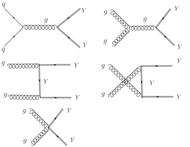
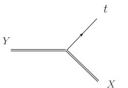
There are four possible combinations of spins that allow a coupling between , and the SM top quark, . These are listed, with the relevant couplings and sample model decays, in Table 1. For fermions we allow a general chirality structure. We shall henceforth refer to these scenarios as models i, ii, iii, and iv.
| sample model and decay | ||||||
| coupling | coupling | |||||
| i | 0, 3 | , 1 | MSSM | |||
| ii | , 3 | 0, 1 | UED | |||
| iii | , 3 | 1, 1 | UED | |||
| iv | 1, 3 | , 1 | [12] | |||
Let us elaborate on the unusual case in which is a vector color triplet, possibly arising as a bound state from strong dynamics or from a special kind of supersymmetric model [12]. The kinetic term is
| (1) |
where . Then the --gluon interaction term is
| (2) |
The resulting Feynman rule is
| (4) |
Likewise, the --gluon-gluon interaction term is
| (5) |
The resulting Feynman rule is
| (7) |
3 Color-Triplet Top-Partner Production
TeV TeV
The dominant modes for production of the top partner in hadronic collisions are the QCD subprocesses
| (8) |
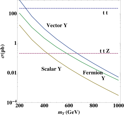
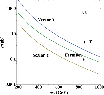
We restrict ourselves to the first- and second-generation quarks and use the CTEQ 6L1 parton distribution functions (PDFs) [13], with the factorization scale set to . For –1000 GeV, the dominant subprocess is , which is about one order of magnitude larger than . The channels are suppressed by roughly one additional order of magnitude.
The total QCD production cross section at the LHC as a function of the mass of the is shown in Fig. 2, for the cases in which has spin , , and . The plots include next-to-leading order (NLO) and resummed next-to-leading logarithmic (NLL) QCD corrections for the scalar [14] and NLO and NNLL corrections for the fermionic [15]. The QCD corrections for vector production have not yet been calculated; we use the -factor for the scalar (1.77 at , 1.56 at ), since the two cases share similar leading-order Feynman diagrams.
The cross section for the fermion is about an order of magnitude larger than that of the scalar, because of the fermion’s extra spin degrees of freedom and threshold effects. In the -channel, the scalar is produced as a -wave with a velocity dependence of , whereas the fermion is produced as an -wave with . Thus, the ratio of the cross sections of the fermion and scalar is larger at small values of , that is, when the mass of the is large. This relative enhancement of the fermionic production is particularly pronounced when the particles are produced mostly near the threshold limit. Note that, although the curves for the vector and scalar appear to be parallel on the logarithmic scale, their ratio varies from about 34 to 16 in the mass range shown.
4 Current Bounds from the Tevatron and LHC
As Fig. 1 indicates, the top-quark partner, , decays to a top quark plus a neutral particle, . The discrete symmetry implies that is stable and leads to missing-energy events. Thus, the signal is plus missing energy. Searches for supersymmetric scalar tops at the Tevatron [16, 17] and the LHC [18, 19, 20] put constraints on the allowed parameter space for the class of processes considered here. Additional, though generally weaker, bounds also arise from general searches for signals with jets and missing energy [21].
Currently, the strongest constraints arise from scalar top searches at ATLAS using 4.7 fb-1 of data taken at [19]. For , they put a lower bound on a scalar . By taking into account the different production cross sections for scalars, fermions, and vectors (see Fig. 2), one can translate the results of Refs. [19] into a limit of for a fermionic top partner and for a vector top.
The bounds are summarized in Table 2. It should be pointed out that the limits for fermionic and vector are simple estimates from theoretical considerations. For more robust results, a detailed experimental analysis of these scenarios needs to be performed.
| Limit on | |
|---|---|
| 0 | |
| 1/2 | |
| 1 |
For larger values of , that is, smaller mass differences , the limits become weaker. The excluded region in the – mass plane for scalar particles will be shown in the next section (see Fig. 4).
5 Signal Observability at the LHC
As the previous section discusses, we consider new physics signals of the type . For the leading channel, in which the top quarks decay hadronically [3], the signal receives large backgrounds from SM processes with multiple QCD jets. To suppress QCD backgrounds, we consider the semileptonic channel [4], in which one of the tops decays hadronically and the other decays leptonically, namely,
| (9) |
This channel is beneficial because of its sizeable branching fraction and the identification of both and . The dominant background processes are
| (10) |
The cross sections for the first two backgrounds (without branching fractions) are shown in Fig. 2 as horizontal lines, including NLO corrections for [22] and NLO+NNLL effects for [23].
The separation of signal and background in the semileptonic channel has been studied previously in the literature [4, 5, 16, 18, 19, 20]. Here, we reanalyze the signal selection with the purpose of developing optimized selection cuts in a phenomenologically realistic simulation setup. Our signal selection follows the strategy of Ref. [4], but we include QCD parton showering and detector smearing effects. As a result, we find that we need to adjust the choice of cuts to account for the effect of QCD radiation***Very recently, several papers have appeared that pursue a similar goal in the context of the MSSM, using traditional selection cuts [6, 8] and top-jet tagging techniques [7]. Our results for the signal observability are comparable to Refs. [6, 7], but significantly better than Ref. [8]..
Jets have been clustered via a cone algorithm with cone size 0.4. To simulate detector resolution effects, we have smeared the jet energy with a Gaussian distribution of width , where is the jet energy in units of GeV. A -tagging efficiency of 70% [24] has been assumed. We have applied the following set of cuts to identify the signal signature and reduce the SM backgrounds.
| (11) |
Here and stand for a jet with or without a -tag, and and are the transverse energy and pseudorapidity of object . describes the angular separation between two jets. is computed from either the or the invariant mass, namely, whichever yields the value closer to the true top-quark mass, , in a given event. is the missing transverse energy.
Events for the partonic signal process and background have been generated with CalcHEP 3.2.5 [25] and passed to Pythia 6.4 [26] for parton showering and jet clustering. The background has been simulated with Pythia. It was shown in Ref. [4] that the background can be reduced effectively with invariant-mass cuts on the for a selection and for a top-quark selection. We have thus neglected this process in our simulation.
With the set of cuts in (11), which we shall refer to as Cut(1), a good signal-to-background ratio is achieved for small values of , when the production cross section is large. For larger values of , additional cuts are required to suppress the SM background sufficiently. It turns out that the following two variables are useful for this purpose: the missing transverse energy, , and the transverse mass of the lepton–missing-momentum system,
| (12) |
The optimal cut values depend on the collider energy:
-
•
For , the choice
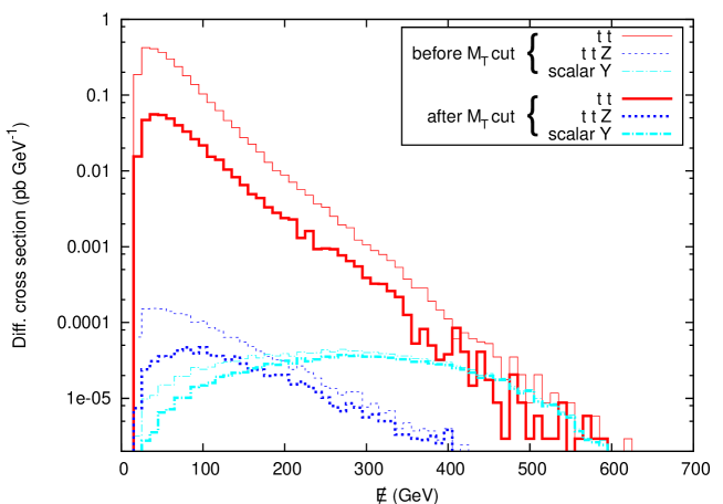
Cut(2h) has been found to be effective for . It can be understood as follows. The cut GeV is necessary because a large amount of missing energy in the SM backgrounds corresponds to neutrinos from the leptonic decay of the W boson. From Fig. 3 one can see that the cut reduces the SM backgrounds dramatically, especially in the low- region. However, the signal events remain virtually the same after this cut: only those in the low- region are slightly affected. Moreover, for the signal there is a plateau between 200 and 400 GeV in Fig 3. The cut 350 GeV has been chosen because above 350 GeV the backgrounds are suppressed considerably. In practice, we have applied either Cut(1) or Cut(2h), whichever produces the larger statistical significance for a given parameter point . Here, and denote the number of signal and background events after cuts.
-
•
For , we have used either Cut(1), or
Cut(2l) or Cut(2l’) whichever results in the largest significance. Cut(2l) and Cut(2l’) have been optimized for and , respectively.
Because the signal cross section is lower for than for , we have lowered the cut to ensure that a sufficient number of signal events passes. However, the looser cut also results in a larger background event yield, so that it is advantageous to apply a stronger cut on to improve the signal significance.
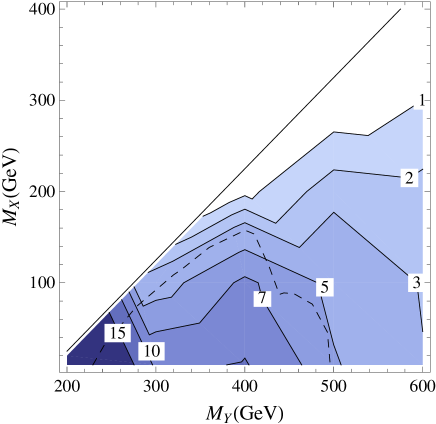
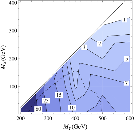
Figure 4 shows the statistical significance that can be achieved with these cuts for model i (scalar and fermionic ), for different values of and . The significance is determined according to if , whereas Poisson statistics is used for very low event yields (). For the other model combinations, ii–iv, the statistical significance can be obtained by scaling the values in Fig. 4 with the production cross sections in Fig. 2.
As the figure shows, the statistical significance is relatively large in the following two regions of the mass plane:
-
1.
Small values of , in which case the signal selection efficiency is almost independent of . Here, the pair, which recoils against an initial-state jet, is typically produced with a sizeable boost. This boost leads to a fairly large missing momentum, which helps to discriminate the signal from the background. Our signal selection works even near the kinematic threshold, where approaches , in contrast to the experimental analysis by ATLAS [19], where such events have been cut away with a strong cut on the azimuthal angle between the leading two jets and the missing momentum†††Note, however, that we generated Fig. 4 by running dedicated simulations for a number of parameter points and using interpolation and extrapolation to cover the entire parameter plane. Consequently, very close to the threshold region (that is, for ) our results may not be reliable..
-
2.
Moderately large values of , , and small values of . For these values of , the pair is produced mostly at rest and the signal selection becomes difficult for small mass differences , when the top quark from the decay is quite soft.
In comparison with Ref. [4], we obtain somewhat lower values for the significance , as a consequence of having performed a more realistic simulation that includes QCD radiation (through parton showering) and jet smearing. These effects make it more difficult to devise clean kinematic selection variables for the signal and result in more background from the tail of smeared distributions. We have also explored the mass reconstruction scheme proposed in Ref. [4] and the variable [27]. We have found them to be useful in certain respects and complementary to the combination of our cuts. Further optimization would depend on detailed (experimental) simulations, which we leave for future studies.
In summary, we have found that, at 14 TeV with an integrated luminosity of 100 fb-1, a scalar top partner can be observed at the 5 level (or better) for a mass up to 675 if . This translates into 945 GeV for a spin-1/2 top partner. At 8 TeV with an integrated luminosity of 20 fb-1, it is possible to achieve a 5 discovery for a scalar top with a mass up to 480. This corresponds to 660 for a spin-1/2 top partner. These results are summarized in Table 3.
| spin-0 | spin-1/2 | |
|---|---|---|
| 8 TeV | ||
| 14 TeV |
6 Determination of Model Properties
6.1 Masses
The independent determination of the and masses in processes of the type
| (13) |
where is a SM fermion, is a difficult problem because of the lack of kinematic features for the under-constrained system. Several methods have been proposed in the literature [28, 27, 29, 30, 31], either based on global event variables such as , on the variable [27] or variants thereof, or on likelihood fits to the complete event information [29]. It was found that, for and a sample of a few tens of thousands of signal events at , the mass difference can be determined to a precision of a few per cent, while the absolute mass scale has an uncertainty of roughly 20–30% [29, 30]. If the state could arise from the decay of a new resonance of known mass, it would help to constrain the kinematics and thus to determine the masses of and as well [31]. More details can be found in the cited papers.
6.2 Spin
The spin of the particle can be probed through the characteristics of the production process. For instance, the production cross section strongly depends on the spin [32]. However, unknown model-dependent branching fractions and the mass uncertainty of order 30% can lead to ambiguities in the determination of the spin from the measured total production rate. Instead, one can largely avoid such problems by investigating the shape of suitable differential distributions. In particular, the two variables described below are effective for this purpose.
-
(1)
Scalar and fermion pair production can be distinguished with the observable
(14) which is constructed from the rapidities of the visible decay products of the hadronically decaying and the leptonically decaying top quarks. In general, there is a combinatorial ambiguity in identifying the -jets and light-flavor jets as the decay products from one of the two top quarks. Given our event reconstruction scheme discussed in the previous section, one can resolve this ambiguity by assuming that the hadronically decaying top quark is made up from the two light-quark jets and the -jet for which is closest to . The remaining -jet and the lepton are then identified as the decay products of the other top quark.
The variable in (14) is closely related to the proposal by Barr in Ref. [33], , where is the pseudorapidity of the SM fermion from the decay . This variable approximately traces the production angle between one and the beam axis in the center-of-mass frame. In the channel, the distribution has a clear dependence on the spin, as can be seen in the formulae
for scalar (spin 0), (15) for fermionic (spin ), (16) where is the velocity of the produced particles. The difference stems from the fact that scalars are produced in a -wave, whereas for fermions the -wave contribution is dominant. In contrast to Ref. [33], the definition (14) is based on the rapidities rather than the pseudorapidities, to account for the fact that the produced top quarks are massive.
In the physical process , only a subdominant fraction of the events originates from annihilation, but as can be seen in Fig. 5 the effect is still noticeable (compare the lines for model i with the other cases).
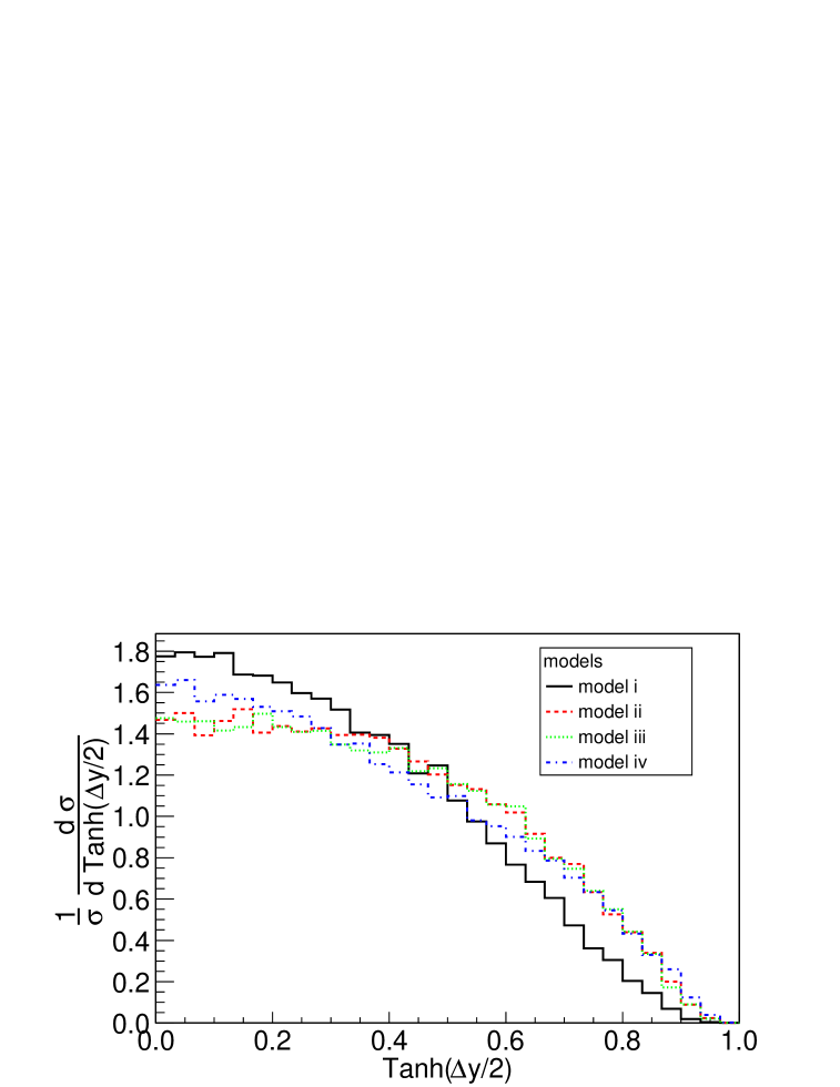
Figure 5: Distribution of for the different top-partner scenarios listed in Table 1, for , , and . For comparison, all distributions have been normalized to unity. -
(2)
There is no appreciable difference between fermionic and vector pair production in the distribution. However, these two cases can be disentangled by means of a variable that measures the effective hard scattering energy [34]. One such observable is the effective mass, a scalar sum over momenta:
(17) where the sum runs over all visible objects (jets and leptons in this case).
The usefulness of this variable follows from the fact that the partonic cross section for the pair production of massive vector particles grows with the partonic center-of-mass energy like , whereas for fermions it has the usual behavior in the high-energy limit. In fact, for very large values of the vector production would violate the perturbative unitarity limit, a sign that additional new massive resonances will appear and modify the production amplitude. The presence of such resonances is generally expected in dynamical models such as the one proposed in Ref. [12]. However, their masses may be beyond the reach of the LHC, depending on the value of when the unitarity limit is eventually reached. We have estimated this limit for vector pair production, conservatively assuming -channel dominance in obtaining . Thus, one can assume that the new heavy resonances have masses of , which make their potential contribution to the process completely negligible, since only a fraction of order of events have partonic center-of-mass energy of this size or larger at .
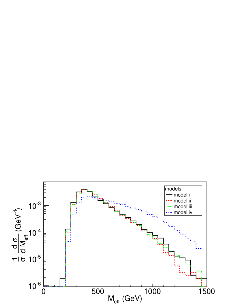
Figure 6: Distribution of for the different top-partner scenarios listed in Table 1, for , , and . For comparison, all distributions have been normalized to unity. The distribution is shown in Fig. 6 for the different model scenarios. A very distinctive difference can be observed between the cases of vector and fermionic or scalar top partners.
Let us quantify the discriminative power of these variable in an example: the process for and at . The simulation and event selection have been performed as described in the previous section, with Cut(1) in Eq. (11). We have assumed the cross section for scalar pair production (model i). Note that this scenario is not ruled out by current LHC results. We have not used the total event rate for model discrimination, to avoid ambiguities due to unknown branching fractions.
We have carried out the discrimination between two different spin assignments by computing the value for the binned and distributions, using three bins in both cases. The result can be expressed in terms of the integrated luminosity necessary for achieving a 5 statistical significance:
| 14 TeV: | scalar versus fermion : | , |
| scalar versus vector : | , | |
| fermion versus vector : | . |
For the current 8 TeV run, a 5 discrimination requires the following integrated luminosities:
| 8 TeV: | scalar versus fermion : | , |
| scalar versus vector : | , | |
| fermion versus vector : | . |
The numbers refer to the purely statistical significance. However, at this level of precision, systematic errors may be important. A potentially large systematic effect stems from the uncertainty of the new-particle masses, and . While the mass difference can be determined rather precisely, the overall mass scale can be measured with only 20–30% accuracy; see section 6.1. We have estimated the effect of this uncertainty by comparing two event samples with and , which differ in by roughly 30%. We have found that this mass uncertainty reduces the statistical significance of the spin discrimination by about 20%; the values of that account for this systematic error are about 50% greater than those quoted above.
In conclusion, the determination of the spin of the top partner, , is possible with very moderate amounts of data. On the other hand, the distinction between models ii and iii, which both have a fermionic but differ in the spin of the singlet , is much more difficult. After surveying more than a dozen different kinematic variables based on the top-quark momenta, we found no significant difference between scenarios ii and iii for any of them. This finding agrees with the results of Ref. [34].
However, more information can be obtained from observables that are sensitive to the top-quark polarization, as will be discussed next.
6.3 Couplings
The chirality structure of the decay (that is, the relative contributions of left- and right-handed chiral couplings) leaves an imprint on the polarization of the top quark, which can be analyzed through angular distributions of the top-quark decay products. This method is particularly effective when the mass difference between and is large (), so that the top quark is energetic and therefore the helicity is preserved, reflecting the chirality. For instance, one can look at the angle () of the quark (lepton) with respect to the top-quark boost direction in the top rest frame. Because the quark is always left-handed, it is emitted predominantly in the forward direction () if the top quark is left-handed, but mostly in the backward direction () if the top quark is right-handed.
In practice, even if the top quark is produced fully polarized in the decay , some of the polarization is washed out by the mass of the top, but the distribution will still exhibit a characteristic difference between left- and right-handed couplings.
In the following, we shall illustrate this behavior using a parton-level simulation with CalcHEP‡‡‡A more realistic simulation at the level of the previous section, including parton showering and signal selection cuts, would require the modification of Pythia to include top-quark spin correlation effects, which we have not attempted to carry out.. We shall focus on the leptonically decaying top quark, since it has a cleaner final state. The top-quark rest frame cannot be reconstructed because of the unobserved neutrino momentum, so we analyze the angular distribution in the rest frame of the visible system instead. The results are shown in Fig. 7.
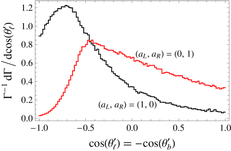
As Fig. 7 shows, the distribution is skewed to smaller values of or, equivalently, larger values of in the case of a left-handed coupling (black curves) than in the right-handed case (red curves). For a mixed case with non-zero left- and right-handed components, one obtains a distribution that lies between the black and red curves. This qualitative behavior is the same for all four spin combinations in Table 1, although they differ from each other in the detailed shape of the distribution. In particular, cases ii and iii have distinctly different shapes; hence, the analysis of this observable may allow one to determine not only the chirality of the coupling but also the spin of the particle. Such a determination is not possible with observables that treat the top quarks as basic objects.
Furthermore, one can probe the chirality even with limited statistics by using two bins and forming the asymmetry
| (18) |
From Fig. 7, one can see that when is about will be most sensitive to the chirality of the coupling. Table 4 shows the asymmetry for models i–iv with two choices of the masses and . The usefulness of for the determination of the coupling is enhanced by its relative insensitivity to the spin and mass combinations.
| GeV, GeV | GeV, GeV | |||||||
| Model | Model | |||||||
| , | i | ii | iii | iv | i | ii | iii | iv |
| 1, 0 | 0.10 | 0.02 | 0.10 | 0.03 | 0 | 0.15 | 0.04 | 0.10 |
| 0, 1 | 0.68 | 0.55 | 0.68 | 0.61 | 0.54 | 0.39 | 0.50 | 0.45 |
| 1, 1 | 0.29 | 0.28 | 0.29 | 0.29 | 0.28 | 0.27 | 0.28 | 0.27 |
7 Conclusions
The SM-like Higgs boson has been observed at the LHC with a relatively light mass of about 125 GeV. The “naturalness” argument of the Higgs sector suggests the existence of partners of the SM particles, especially the heavy top quark. The top quark may thus hold the key to new physics associated with the electroweak symmetry-breaking sector, because of its enhanced coupling to the Higgs sector. In this paper, we have systematically categorized the generic interactions of a new particle that couples to the top quark and a stable neutral particle, which serves as a candidate for cold dark matter. We have considered all possible assignments of spin 0, and 1 for either of the two new particles.
In the search for new physics involving top quarks and its partners at the LHC, the experimental signatures may be distinctive, but challenging to disentangle. Pair production of the massive top partners leads to a signature of a pair plus missing energy, which is difficult to separate from the large SM background. We have presented a set of optimized selection cuts for isolating this new physics signal at the 8 and 14 TeV runs of the LHC. We have found that, at 14 TeV with an integrated luminosity of 100 fb-1, a spin-zero top partner can be observed at the 5 level up to a mass of 675 GeV, while for a spin- top partner the reach extends to 945 GeV.
If a process of this type is discovered at the LHC, it will be imperative to determine the spins and couplings of the new particles, in order to understand the underlying physics mechanism. We have proposed a strategy to extract these properties from experimental data by means of suitable differential distributions of the final-state products. With this approach, a spin-0 top partner with mass of about 300 GeV can be discriminated from spin- and spin-1 particles at the 5 level with a luminosity of 10 fb-1 at 14 TeV. Furthermore, the structure of the coupling that mediates the decay of the top partner into a top quark and a massive neutral particle can be analyzed by measurement of the polarization of the final-state top quarks. This method allows one to distinguish clearly between left-handed, right-handed, and vector couplings. Most importantly, the proposed observables for spin and coupling determination are insensitive to unknown branching fractions and depend only mildly on the masses of the new particles.
In conclusion, the LHC will allow us to observe and study top partners with mass up to about 1 TeV. This program will shed light on the interplay of the Higgs-boson and top-quark sectors and may elucidate the concept of naturalness.
Acknowledgements
We are grateful to M. Cacciari and A. Kardos for providing background cross sections at 8 TeV. We also thank N. Christensen for help with CalcHEP and R. Mahbubani for correspondence. This project was supported in part by the National Science Foundation under grant PHY-0854782, by the US Department of Energy under grant No. DE-FG02-12ER41832, and by PITT PACC. C.-Y.C was supported in part by the George E. and Majorie S. Pake Fellowship. Finally, T.H. is grateful for the hospitality and support of the Aspen Center for Physics and the Center for Theoretical Underground Physics and Related Areas (CETUP*) during the completion of this work.
References
- [1] J. Incandela [for the CMS Collaboration] and F. Gianotti [for the ATLAS Collaboration], talks at CERN LHC seminar, July 4, 2012 [http://indico.cern.ch/event/197461].
- [2] G. F. Giudice, in “Perspectives on LHC physics,” eds. G. Kane, A. Pierce, 155–178 [arXiv:0801.2562 [hep-ph]].
- [3] P. Meade and M. Reece, Phys. Rev. D 74, 015010 (2006).
- [4] T. Han, R. Mahbubani, D. G. E. Walker and L.-T. Wang, JHEP 0905, 117 (2009).
-
[5]
T. Plehn, M. Spannowsky, M. Takeuchi and D. Zerwas,
JHEP 1010, 078 (2010);
T. Plehn, M. Spannowsky and M. Takeuchi, JHEP 1105, 135 (2011). -
[6]
Y. Bai, H.-C. Cheng, J. Gallicchio and J. Gu,
arXiv:1203.4813 [hep-ph];
D. S. M. Alves, M. R. Buckley, P. J. Fox, J. D. Lykken and C. -T. Yu, arXiv:1205.5805 [hep-ph];
Z. Han, A. Katz, D. Krohn and M. Reece, arXiv:1205.5808 [hep-ph];
D. E. Kaplan, K. Rehermann and D. Stolarski, arXiv:1205.5816 [hep-ph]. - [7] T. Plehn, M. Spannowsky and M. Takeuchi, arXiv:1205.2696 [hep-ph].
- [8] J. Cao, C. Han, L. Wu, J. M. Yang and Y. Zhang, arXiv:1206.3865 [hep-ph].
- [9] B. Dutta, T. Kamon, N. Kolev, K. Sinha and K. Wang, arXiv:1207.1873 [hep-ph].
- [10] See, for example, S. P. Martin, in “Perspectives on supersymmetry II,” ed. G. L. Kane, World Scientific, Singapore (2010), 1–153 [hep-ph/9709356].
-
[11]
T. Appelquist, H. C. Cheng and B. A. Dobrescu,
Phys. Rev. D 64, 035002 (2001);
B. A. Dobrescu and E. Pontón, JHEP 0403, 071 (2004);
G. Burdman, B. A. Dobrescu and E. Pontón, JHEP 0602, 033 (2006). - [12] H. Cai, H.-C. Cheng and J. Terning, Phys. Rev. Lett. 101, 171805 (2008).
- [13] J. Pumplin, D. R. Stump, J. Huston, H. L. Lai, P. M. Nadolsky and W. K. Tung, JHEP 0207, 012 (2002).
- [14] W. Beenakker, S. Brensing, M. Krämer, A. Kulesza, E. Laenen and I. Niessen, JHEP 1008, 098 (2010).
- [15] M. Cacciari, M. Czakon, M. L. Mangano, A. Mitov and P. Nason, Phys. Lett. B 710, 612 (2012).
- [16] T. Aaltonen et al. [CDF Collaboration], Phys. Rev. Lett. 106, 191801 (2011).
-
[17]
V. M. Abazov et al. [D0 Collaboration],
Phys. Lett. B 693, 95 (2010);
M. S. Carena, J. Hubisz, M. Perelstein and P. Verdier, Phys. Rev. D 75, 091701 (2007). - [18] G. Aad et al. [ATLAS Collaboration], Phys. Rev. Lett. 108, 041805 (2012).
-
[19]
G. Aad et al. [ATLAS Collaboration],
ATLAS-CONF-2012-071;
G. Aad et al. [ATLAS Collaboration], ATLAS-CONF-2012-073;
G. Aad et al. [ATLAS Collaboration], ATLAS-CONF-2012-074. -
[20]
S. Sharma [for the CMS Collaboration],
talk at the 36th International Conference for High Energy Physics (ICHEP
2012), Melbourne, Australia, 4–11 July 2012;
C. Rogan [for the CMS Collaboration], talk at the 36th International Conference for High Energy Physics (ICHEP 2012), Melbourne, Australia, 4–11 July 2012. -
[21]
R. Essig, E. Izaguirre, J. Kaplan and J. G. Wacker,
JHEP 1201, 074 (2012);
Y. Kats, P. Meade, M. Reece and D. Shih, JHEP 1202, 115 (2012);
M. Papucci, J. T. Ruderman and A. Weiler, arXiv:1110.6926 [hep-ph];
X.-J. Bi, Q.-S. Yan and P.-F. Yin, Phys. Rev. D 85, 035005 (2012);
C. Brust, A. Katz, S. Lawrence and R. Sundrum, JHEP 1203, 103 (2012);
N. Desai and B. Mukhopadhyaya, JHEP 1205, 057 (2012);
A. Choudhury and A. Datta, arXiv:1207.1846 [hep-ph]. -
[22]
A. Lazopoulos, T. McElmurry, K. Melnikov and F. Petriello,
Phys. Lett. B 666, 62 (2008);
A. Kardos, Z. Trocsanyi and C. Papadopoulos, Phys. Rev. D 85, 054015 (2012);
M. V. Garzelli, A. Kardos, C. G. Papadopoulos and Z. Trocsanyi, Phys. Rev. D 85, 074022 (2012). - [23] M. Beneke, P. Falgari, S. Klein and C. Schwinn, Nucl. Phys. B855, 695 (2012).
- [24] G. Aad et al. [ATLAS Collaboration], arXiv:1205.2067 [hep-ex].
-
[25]
A. Pukhov,
hep-ph/0412191;
A. Pukhov, A. Belyaev, N. Christensen, http://theory.sinp.msu.ru/~pukhov/calchep.html. - [26] T. Sjöstrand, S. Mrenna and P. Z. Skands, JHEP 0605, 026 (2006).
- [27] C. G. Lester and D. J. Summers, Phys. Lett. B 463, 99 (1999).
-
[28]
For an overview, see
sect. 4 in A. J. Barr and C. G. Lester, J. Phys. G 37, 123001 (2010), and refs. therein;
sect. X in A. J. Barr, T. J. Khoo, P. Konar, K. Kong, C. G. Lester, K. T. Matchev and M. Park, Phys. Rev. D 84, 095031 (2011), and refs. therein. - [29] J. Alwall, A. Freitas and O. Mattelaer, AIP Conf. Proc. 1200, 442 (2010).
-
[30]
P. Konar, K. Kong, K. T. Matchev and M. Park,
Phys. Rev. Lett. 105, 051802 (2010);
T. Cohen, E. Kuflik and K. M. Zurek, JHEP 1011, 008 (2010). - [31] T. Han, I. -W. Kim and J. Song, Phys. Lett. B 693, 575 (2010); arXiv:1206.5633 [hep-ph]; arXiv:1206.5641 [hep-ph].
- [32] G. L. Kane, A. A. Petrov, J. Shao and L. T. Wang, J. Phys. G 37, 045004 (2010).
- [33] A. J. Barr, JHEP 0602, 042 (2006).
- [34] C.-Y. Chen and A. Freitas, JHEP 1102, 002 (2011).