NORDITA-2012-57
UUITP-20/12
Large Limit of Gauge
Theories from Localization
J.G. Russo1,2***On leave of absence from Universitat de Barcelona and Institute of Cosmos Sciences, Barcelona, Spain. and K. Zarembo3,4†††Also at ITEP, Moscow, Russia.
1 Perimeter Institute for Theoretical Physics,
Waterloo, Ontario, N2L 2Y5, Canada
2 Institució Catalana de Recerca i Estudis Avançats (ICREA),
Pg. Lluis Companys, 23, 08010 Barcelona, Spain
3Nordita,
Roslagstullsbacken 23, SE-106 91 Stockholm, Sweden
4Department of Physics and Astronomy, Uppsala University
SE-751 08 Uppsala, Sweden
jorge.russo@icrea.cat, zarembo@nordita.org
Abstract
We study Yang-Mills theory on in the large- limit. We find that on a large sphere Wilson loops obey a perimeter law and that the free energy grows quadratically with the radius of the sphere. We also comment on the large- limit of the theory, and on the free energy in and superconformal theories.
1 Introduction
In supersymmetric field theories a certain class of non-trivial dynamical quantities can be computed exactly. An example, that we will further explore here, is the partition function of an supersymmetric gauge theory on . By using localization, the partition function can be reduced to a finite-dimensional matrix integral [1]. Observables, that can be computed by this method, include the free energy and expectation values of circular Wilson loops.
One can envision a number of applications of this remarkable result. The ’t Hooft’s large- limit of the matrix integral [2, 3, 4, 5, 6] may give us a glimpse on the putative string duals of theories. In particular, for the super-Yang-Mills theory (SYM), localization confirms earlier conjectures on the circular Wilson loop [7, 8], which were instrumental in verifying the AdS/CFT correspondence. Or one can address generic questions about quantum field theory, such as the asymptotic behavior of perturbative series [6] in the setting where exact non-perturbative results are available.
We will study the large- limit of the Pestun’s matrix model, focusing on the simplest example of asymptotically free gauge theory, pure SYM. When the radius of the four-sphere becomes infinite we will be able to compare our results to the large- limit of Seiberg-Witten theory [9], which was analyzed in [10, 11]. We will also comment on the theory (a massive deformation of ), which was studied in [6], and on the superconformal theories considered in [2, 3, 4, 5]. The motivation here is the AdS/CFT duality, and we will fill the gap in the literature by computing the finite part of the holographic free energy in SYM.
What do we expect to find, when we study an asymptotically free QFT on ? In absence of other parameters in the problem, the dynamics is controlled by the running coupling renormalized at the inverse size of the sphere (). When the radius is small, perturbation theory should work and yield an expansion of observables in inverse powers of . For a large sphere, the theory enters a non-perturbative regime, and the behavior of observables becomes a non-trivial dynamical question. We know that SYM is not confining [9], and may thus expect that Wilson loops will obey a perimeter law, rather than an area law. As for the free energy, it cannot be extensive (cannot scale as ), because the vacuum energy is strictly zero in any supersymmetric theory. Since the perturbative free energy quadratically diverges in SYM (see footnote 1), we may expect to find a behavior, where the UV cutoff is replaced by the dynamically generated mass scale . The analysis of the matrix model will confirm these expectations.
2 SYM
2.1 Partition function
The partition function of any supersymmertic gauge theory on is calculable by localization methods [1]. The end result of this calculation is a finite-dimensional integral over the moduli space of Coulomb vacua, parameterized by the eigenvalues of the scalar field from the vector multiplet: , . We will mostly concentrate on the simplest example, pure Yang-Mills theory without matter multiplets. Its partition function is given by the eigenvalue integral
| (2.1) |
The key point in the localization method is the one-loop exactness of the effective action for the eigenvalues. It thus suffices to compute one-loop determinants and to sum over instantons.
The one-loop factor was calculated in [1] and is expressed in terms of the function , defined as an infinite product over spherical harmonics:
| (2.2) |
The coupling constant in the partition function is actually the running coupling renormalized at the scale set by the radius of the sphere, the only parameter in the problem. Of course, the original path integral before localization depends on the bare coupling , but this combines with the one-loop UV logarithms to produce the renormalized running coupling . Indeed, the product over spherical harmonics appears in the calculation of [1] without the suppression factor and thus logarithmically diverges. The infinite contribution, cut off at some is absorbed by renormalizing the bare coupling:
| (2.3) |
as can be easily seen from (2.1) ( is the Euler constant). A more mathematically precise way to get rid of divergences, used in [1] and also discussed later in section 4, is to consider theory as a UV completion of pure SYM. The mass of the adjoint hypermultiplet then plays the rôle of the UV cutoff .
The running coupling can be expressed through the radius of the sphere and the dynamically generated finite scale :
| (2.4) |
The running coupling becomes negative at . What makes the integral in (2.1) convergent is the rapid decrease at infinity of the one-loop function .
Although it is commonly assumed that instantons are unimportant at large-, this is guaranteed to be true only at weak coupling. In principle the entropy (the volume of the instanton moduli space) may overcome the exponential suppression by the instanton action. Then the instanton weight becomes exponentially large, and the system undergoes a transition to a new phase. Whether such transition happens or not is a dynamical question [12]. Such an instanton-induced phase transition does not occur in the superconformal theory [3]. This dynamical question is more intricate in the SYM case, where the coupling runs and it is not clear a priori which is the relevant scale for appearing in the instanton weight. As explained below, the scale at which the coupling is renormalized, can get dynamically shifted from . The new scale effectively represents the inverse of the instanton size, and a relevant question is whether the partition function is dominated by small or large instantons. These issues will be addressed in section 5, where the instanton factor in the large limit is discussed. Meanwhile, we will first set to , and in section 5 we will argue that indeed it is not relevant for the large dynamics by explicitly computing the one-instanton contribution.
Supersymmetric observables map, upon localization, onto expectation values in the matrix model. For example, the Wilson loop in the fundamental representation on the big circle of maps to the trace of the matrix exponential:
| (2.5) |
Our goal is to solve the matrix model in the large- limit and to compute the free energy and the Wilson loop vacuum expectation value (VEV).
2.2 Toy model:
Before proceeding with the large- calculation, it is instructive to consider the partition function, which is given by a simple one-dimensional integral:
| (2.6) |
which we will compute in the saddle-point approximation. As we will explain, the saddle-point approximation is not arbitrarily accurate for , but numerically works pretty well. A more serious problem is that one cannot really ignore instantons at small , so this is just a toy model that illustrates the effect of the one-loop determinant. It gives a correct qualitative picture of what happens in the theory at large .
The saddle point of the integral (2.6) is determined by a minimum of the effective potential:
| (2.7) |
Here we ignore a term coming from the Vandermonde determinant, which can be viewed as a quantum prefactor. It is not significant for the large behavior.
The function has the following large and small asymptotics:
| (2.8) |
The coupling constant here is renormalized at the inverse radius of the sphere , but only at small . When is large, behaves as and a new scale emerges. The effective potential thus has the Coleman-Weinberg shape [13], illustrated in fig. 1.
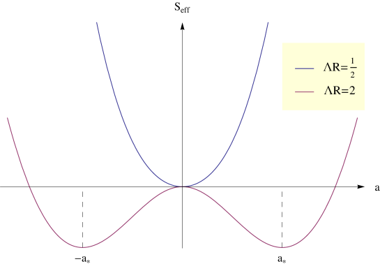
The potential has a minimum at zero for (which is slightly shifted off zero if the Vandermonde determinant is included). However, if , this point becomes a maximum, and the saddle point shifts to a solution of the equation:
| (2.9) |
where
| (2.10) |
and . The saddle-point equation is essentially the condition . For large radius, the saddle-point position thus grows approximately linearly with , (the saddle-point approximation applies when the second derivative of the potential is large; in the present case, ).
The VEV of the circular Wilson in the saddle-point approximation is given by . Since at , the Wilson loop stays constant at small , within the semiclassical approximation. In practice, the exact VEV slowly grows with until reaches , after which and the Wilson loop starts growing very fast. Asymptotically, at very large ,
| (2.11) |
The Wilson loop thus satisfies the perimeter law, and the free energy is quadratic in the radius of the sphere. We will find the same behavior in the SYM at large .
The perimeter law means that the mass of a heavy probe, associated with the Wilson loop, acquires a finite negative renormalization. The quadratic dependence of the free energy on the radius can be interpreted as a finite renormalization of the Newton’s constant. In fact, a short-distance, quadratically divergent contribution to the Newton’s constant does not vanish in the pure theory111This can be seen by setting in eqs. (11), (15) and (18) in [14].. The quadratic dependence of the free energy on the dynamically generated scale can be viewed as a finite remnant of this quadratic UV divergence.
2.3 Saddle-point equation
At large , the eigenvalue distribution is characterized by a continuous density , defined on a interval . The integral (2.1) is dominated by an eigenvalue distribution determined by the saddle-point equation
| (2.12) |
The eigenvalue density is subject to the normalization condition
| (2.13) |
We now study the solutions to (2.12) in different regimes.
Small radius
When , one has . This is the perturbative regime. In this region, the linear force represented by in (2.12) pushes all eigenvalues near . As a result, and we can use the expansion of in powers of ,
| (2.14) |
The solution of the eigenvalue density equation (2.12) is then of the form
| (2.15) |
where is determined by the perturbative order that one wishes to compute. Then (2.15) is a solution to (2.12) with defined by the sum (2.14) truncated at the same .
Substituting the ansatz (2.15) in (2.12) we find an equation of the form . This gives conditions for unknowns, . Then is found by the normalization condition.
Let us explicitly work out the case . Using the formulas,
| (2.16) |
| (2.17) |
one gets a linear system of equations for . Substituting the solution in the normalization condition leads to a polynomial equation for which can be solved in a power series in ,
| (2.18) |
The expectation value of the circular Wilson loop (2.5) is then computed from the formula
| (2.19) |
This gives a linear combination of and Bessel functions. Expanding in powers of , we obtain the perturbative series
| (2.20) |
This may be compared with explicit evaluation of Feynman diagrams, except that the matrix-model calculation is enormously easier and in principle can be pushed to an arbitrary order in . It is interesting to notice that the expansion can be organized differently, without expanding the Bessel functions in . This would give
| (2.21) | |||||
Considering the leading term in , , the first term in this expansion is the Wilson loop VEV in the SYM, which is known to resum an infinite series of Feynman diagrams without internal vertices [7, 8]. The part in (2.20) can be easily recognized as those terms that have no function coefficients. This part of the series has an infinite radius of convergence.
It would be very interesting to determine the asympotic behavior of the full series in (2.20). It is believed that in gauge theories the number of planar graphs of th order grows like a power of , as opposed to the total number of Feynman diagrams [Makeenko:2002uj]. This indicates that, if the coefficient of the term grows as , as occurs in the cases studied in [6], it would be be due to UV renormalons.222 Infrared renormalons arise from the small momentum part of the loop integrals in a certain subset of -loop Feyman diagrams. They should not appear in the present context because the radius of the sphere provides an IR cutoff; integrals over momenta are replaced by sums over spin 0, 1/2, and 1 spherical harmonics of . In this case the planar series (2.20) would be Borel summable, since UV renormalons should not produce poles on the real positive axes of the Borel plane (this expectation is consistent with the alternating sign character of the series).
Large radius
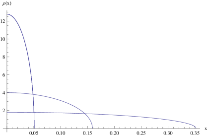
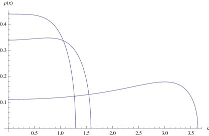
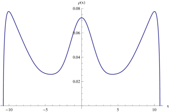
At large radius the running coupling becomes small and negative. In this regime the eigenvalues are strongly repelled from the region around zero. The effective potential for an individual eigenvalue looks like the lower curve in fig. 1. We can imagine two possibilities in this case. If the potential wells near the minima are sufficiently deep, the eigenvalue distribution will consist of two disconnected patches. Clearly, a two-cut solution cannot be continuously connected to the one-cut solution at weak coupling. In this case there will be a large- phase transition at some critical coupling. We found, however, (numerically) that this scenario is not realized in SYM. The effective potential is always sufficiently shallow, such that the short-distance repulsion between the eigenvalues spreads them along a single connected interval for any . For a negative above some critical value, the eigenvalue density gets a double-hump structure with a dip in the middle, shown in fig. 2.
The extent of the eigenvalue distribution grows rapidly as (exponentially in or linearly in ). The series expansion (2.14) is useless in this regime, because its radius of convergence is equal to one. In appendix A we illustrate this point by considering a toy model obtained by truncating the series (2.14). The model exhibits a phase transition at a finite and, as a result, the resulting large radius behavior is markedly different from the behavior in the actual eigenvalue density in theory.
We can solve the saddle-point equation (2.12) asymptotically in the limit , i.e. , where . The density will then take a scaling form: , everywhere apart from tiny regions near the endpoints. Using the asymptotic form of the kernel:
| (2.22) |
we can see that in the scaling limit the Hilbert kernel scales away, and we are left with the equation
| (2.23) |
Differentiating this equation twice, we then get:
| (2.24) |
This equation has a unique normalizable solution:
| (2.25) |
This can be seen to agree with the eigenvalue density [10, 11] obtained from Seiberg-Witten theory directly in flat space.
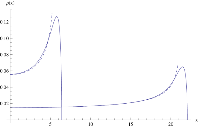
As we will see from the numerics, shown in fig. 3, the analytic solution represents a very good approximation to the large radius eigenvalue density, apart from a small region near the endpoints, where it violates the boundary conditions.
Returning to the original equation, one can calculate that
| (2.26) |
Consequently,
| (2.27) |
Let us now compute the expectation value of the circular Wilson loop and the free energy in this large radius regime. Using the asymptotic analytic formula (2.25) and (2.19), we obtain
| (2.28) |
As in the case, we obtain a perimeter law. The leading behavior can be interpreted as negative mass renormalization for a heavy probe particle going around the circular loop. In terms of the running coupling constant, this is
| (2.29) |
To compute the free energy, we start with the relation
| (2.30) |
At large , using the asymptotic density,
| (2.31) |
Therefore
| (2.32) |
at .
Numerical solution
We start with small values of , where we know the detailed analytic form of the solution. We consider the ansatz
| (2.33) |
By taking sufficiently large, one can achieve any desired accuracy, as long as the solution contains only one cut. We have computed the different coefficients and numerically for , and checked that the numerical solution is stable under further increasing .

Consider first the interval , corresponding to . Fig. 2a shows the eigenvalue density for . The eigenvalue distribution expands as is increased. The same qualitative shape is maintained by further increasing up to , where has a finite value . As the equation (2.12) has an analytic dependence on the parameter , there is no discontinuity in crossing from to the region . Thus, at , the eigenvalue density coincides with . The interesting behavior arises for larger values of . The repulsive force becomes stronger and the eigenvalues are repelled from the region of small . This can be seen in fig. 2b, which shows the eigenvalue density for .
The numerical results show that, unlike the toy model of appendix A, the one-cut solution exists for all values of . There is no phase transition. When is negative and approaches to , in the present case begins to increase exponentially with (therefore linearly with ); the eigenvalue distribution gets stretched out, up to a value , with an eigenvalue density that, as , approaches the asymptotic form (2.25). This is shown in fig. 3, which displays the eigenvalue density for along with the analytic asymptotic eigenvalue density (2.25). We see that there is a good agreement between the numerical and analytic curves away from the boundary , an agreement which is clearly better for .
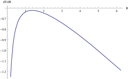
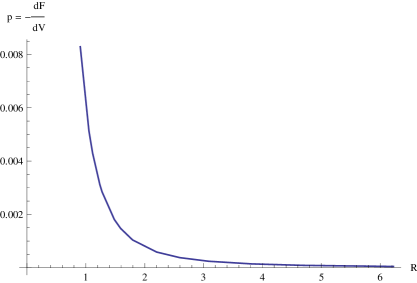
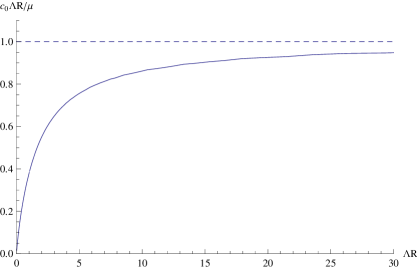
Fig. 4a shows as a function of . This figure illustrates in particular that the point is not special, as is smooth at this point. It also exhibits the linear law at large , obtained analytically in the previous subsection. Fig. 4b shows that the slope of the curve asymptotically approaches the constant found earlier. Note that the linear behavior of is a good approximation even in the region .
Finally, fig. 5a shows the derivative of the free energy as a function of . At it exhibits the linear behavior found analytically in the previous subsection. At , it has the behavior , as it can be easily deduced from the perturbative formulas. We notice that there is a change of sign in at the critical radius where . A natural question is whether this has any thermodynamic implication. The pressure of the system is , where is the volume of , . In stable systems, the pressure must be positive and, in most common systems, also the compressibility, , is positive. This is also the case in the present system, as shown in fig. 5b: the pressure has positive sign in the whole interval . The same plot shows that the compressibility is always positive.
In conclusion, we have seen that the one-cut solution exists for all values of . We have also checked that there are no two-cut solutions at any (see also discussion at the end of appendix A).
3 Remarks on superconformal theories
The simplest superconformal theory (SCYM) is SYM with hypermultiplets in the fundamental respresentation. The large- limit of SCYM on was studied in [2, 3, 4, 5], with the idea to get an insight into its putative AdS dual. One may expect that in the strong coupling limit it should behave similarly to SYM. Quite surprisingly, the strong-coupling limit of the theory is very different from . The free energy tends to a constant rather than growing logarithmically [4], while the Wilson loop VEV grows as a cube of the ’t Hooft coupling [3], in a stark contrast to the exponential growth in the SYM.
Below we will comment on the computation of the free energy in SCYM, in SYM and in its holographic dual. The holographic computation is a classic result in AdS/CFT [15]. Yet, we were unable to find a holographic derivation of the dependence in the literature, and so we will derive this result by reinterpreting the formulas in [15]. We will argue that the logarithm arises due to a subtle difference between field-theory and supergravity UV cutoffs.
3.1 SYM
The SYM localizes to the Gaussian matrix model, whose exact eigenvalue density is given by Wigner semi-circle law:
| (3.1) |
The free energy then is
| (3.2) |
a result which is easy to obtain directly from the Gaussian matrix integral.
represents the integrated one-point function of the action density (more generally, is related to the integrated -point function of the action density). Since , the result is independent of the normalization of , as long as there is no extra -dependent normalization factor. This requirement is equivalent to saying that the measure does not depend on .
3.2 Holographic calculation
At strong coupling, the free energy of SYM is identified with the on-shell supergravity action on :
| (3.3) |
where is the 5d Newton’s constant, is the radius of the Anti-de-Sitter space, and contains the Gibbons-Hawking surface term and boundary counterterms, necessary to eliminate the divergences.
The metric of , foliated such that the boundary is , assumes the following form:
| (3.4) |
The boundary is the large four-sphere at . Using the Einstein’s equations, , the action is calculated to be [15]:
| (3.5) |
where is the supergravity cutoff. The counterterms cancel off quartic, quadratic and logarithmic divergences in this expression. The explicit expressions can be found in [15, 16].
Let us concentrate on the logarithmically divergent term:
| (3.6) |
The counterterm that eliminates this log-divergence is also responsible for the trace anomaly in the energy-momentum tensor [17, 18], so the coefficient in front is directly related to the conformal anomaly of SYM. Once this coefficient is expressed in terms of of the according to the AdS/CFT dictionary:
| (3.7) |
it precisely matches with a logarithmic divergence that is also present in the partition function of on [14].
The common lore of the AdS/CFT duality is that one should first eliminate divergences by adding counterterms [19] and then compare finite quantities. For the free energy one would then obtain a -independent constant, in a clear contradiction with the field-theory calculation. We are going to argue that the reason for this mismatch is a (finite and calculable) difference between the field-theory and supergravity counterterms, that follows from the energy-radius relation for the AdS metric [20].
We will relate the supergravity cutoff with the field-theory cutoff by a simple physics argument [20]. Consider an theory broken down to by pulling one brane out of the stack that creates AdS and placing it at some radial distance away from the horizon. The W-boson, associated with broken symmetry, is described by a string stretching from the horizon to the brane. Consider now the W-boson with the largest possible mass. The upper bounds on the mass, both in field theory and in supergravity, arise from the UV regularization. In field theory, the largest possible mass is obviously . We can express through by computing what is the largest possible mass in supergravity. In order to do that we consider a heavy probe with the largest attainable mass moving along the big circle of . On the field theory side, the action of the heavy probe is . The string action (the area of the worldsheet stretching from the horizon to the cutoff surface along the big circle, fig. 6) is
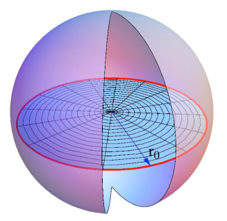
| (3.8) |
from which we conclude that
| (3.9) |
where in the last equality we used the standard AdS/CFT relationship between the radius of and the ’t Hooft coupling of SYM. The necessity to introduce in the energy-radius relation can be also seen from the (constant) Weyl rescaling that brings the near-horizon metric of the D3 brance into the canonical form [21].
Combining (3.6), (3.7) and (3.9), we thus express the free energy in terms of the field-theory quantities:
| (3.10) |
The second, infinite piece is renormalized away upon deriving the matrix model by localization333We were informed by V. Pestun that the dependence on , and consequently on can be easily reconstructed for a generic theory, with the coefficient equal to the -type anomaly. In particular, in SYM, the -dependence is consistent with (3.10).. The finite piece reproduces (3.2).
3.3 SCYM
Consider now the superconformal theory with fundamental massless flavors. The partition function is
| (3.11) |
which leads to the following saddle-point equations:
| (3.12) |
The asymptotic solution at infinite coupling can be found by Fourier transform [3]:
| (3.13) |
The free energy at strong coupling follows then from :
| (3.14) |
The next correction, as argued in [4], is proportional to . We will compute the coefficient of proportionality and also the next term in the expansion.
The asymptotic density extends to infinity, but at any finite the density is supported on a finite interval , where is determined by the equation [3]:
| (3.15) |
where444An analytic expression for the constant in terms of an infinite sum is given in [3].
The deviation of the density from its asymptotic form leads to corrections to , which are calculated in appendix B:
| (3.16) |
where The origin of these two terms is easy to understand. The asymptotic density, which extends all the way to infinity, underestimates the number of small eigenvalues, the true eigenvalue distribution is more compressed. Hence the negative sign of the first correction. However, in addition to an overall increase in the density between and , which is the leading effect, there is a short-range pile up of the eigenvalues near the endpoints, which produces the next term with the positive sign.
Integrating the free energy with the help of (3.15), which, at this order, amounts to setting , we get the final result:
| (3.17) |
This is obviously very different from the simple behaviour in , which is exact and is valid at any coupling. In the SCYM, the free energy is a non-trivial function of , and behaves logarithmically only in the weak-coupling limit.
4 Remarks on theory
This theory is obtained by deformation of SYM by adding a mass555Here the radius of the sphere is absorbed into the definition of the mass of the hypermultiplet: . term for the adjoint hypermultiplet. In this case the equation for the eigenvalues is
| (4.1) |
Now the eigenvalue density depends on a two-parameter space . Some corners of this two-parameter space were studied in [6]. For small , it approaches the eigenvalue density of SYM plus corrections,
| (4.2) |
for and . In particular, one finds and
| (4.3) |
For large and fixed , the theory flows to the SYM theory studied in section 2, with renormalized coupling defined by . To show this explicitly, we take the large limit, where one can approximate
| (4.4) |
Thus, neglecting contributions, we have
| (4.5) |
Using
| (4.6) |
and , we are left with the saddle-point equation (2.12) for the pure SYM theory.
Returning to the theory, by solving the saddle-point equation (4.1) numerically one can also explore other regions of the two-parameter space , away from the corners represented by the and SYM theories. One novel feature with respect to the theory studied in section 2 is that, for a wide range of parameters, eigenvalues accumulate near and near at the same time.
This is illustrated by fig. 7. It exhibits a hill at and two more at . As is further increased, the hill at diminishes, and increases, approaching the eigenvalue density of theory studied in the previous section.
We have also checked that in SYM theory the one-cut solution exists in all regions of the parameter space and that there are no two-cut solutions in any region of the parameter space.
5 Instanton contributions
Instanton contributions are usually believed to be negligible at large , because of the exponential factor in the instanton weight. It is possible, however, that the instanton moduli integration overcomes this exponential suppression making the instanton contribution formally divergent in the large- limit. This phenomenon leads to an instanton-induced phase transition [12]. It was shown in [3] that such a transition does not happen in the superconformal theory discussed in sec. 3.3 and that the instantons always remain exponentially suppressed in SCYM. Here we analyze the instanton weight in the pure SYM.
The expression for the instanton factor in pure SYM theory can be obtained by taking a suitable limit of the instanton weight in theory. When regarding the theory as a UV regularization of the pure SYM some care is necessary in picking the same renormalization scheme in all parts of the localization partition functions. By that we mean the use of the same definition for the running coupling, which is a priori ambiguous due to the choice of the subtraction point. As in sec. 4, we adopt the following definition:
| (5.1) |
where represents the bare coupling of and as before denotes the running coupling constant of the theory. We emphasize that once we have used this renormalization prescription in evaluating the perturbative part of the partition function, the definition of the running coupling in the instanton weight is not a matter of choice any more. We should use the same definition. In particular, the dynamically generated scale,
| (5.2) |
is then given by
| (5.3) |
The pure SYM without matter multiplets arises in the limit , with fixed. The one-instanton contribution to the partition function of the theory can be found e.g. from the expression given in [22] (which is a particular case of the Nekrasov partition function [23, 24]):
| (5.4) |
Here is the theta-angle of the theory. Another possible representation is through a contour integral:
| (5.5) |
where the contour of integration encirlces the poles at counterclockwise.
Upon taking the limit , with fixed, the instanton weight (5.5) becomes
| (5.6) |
with the renormalized coupling given by (5.1). Remarkably, for odd , the theta-angle also gets renormalized:
| (5.7) |
We recall that the running coupling becomes negative at . In such a situation, the factor does not suppress the instanton contribution, but, on the contrary, enhances it! One might naively conclude that instantons become very important at large if .
To clarify this important point, we need to compute . In the large- limit, the instanton weight becomes
| (5.8) |
where the integration can now be taken along the real axis, and
| (5.9) |
The -integral is of the saddle-point type, with the single saddle-point at , so we find that
| (5.10) |
with
| (5.11) |
The instantons are suppressed if and only if for any value of , which is not at all obvious as the first term becomes negative for . We have checked that the full action is nevertheless positive for any , by computing the action analytically in the two limiting cases of and and numerically at intermediate ’s.
At small , the integral in (5.11) can be estimated as . The action thus is large and positive. Obviously, as grows, the action will diminish (at first logarithmically). The question is whether it crosses zero or not. To answer this question we can study the opposite limit of very large .
When , the bare instanton weight, and , which would naively imply that the one-instanton contribution blows up at , but we also need to take into account the last term, the matrix-model average of . Since we know the solution of the matrix model analytically at , we can take this solution and calculate the integral. Inserting from (2.25), and taking into account that , we get:
| (5.12) | |||||
Using the explicit expression for from (2.27), we finally get
| (5.13) |
The instanton action becomes very small at large , but remains positive.
We have checked numerically that the instanton action is a monotonic function of and consequently never becomes smaller than zero. In conclusion, in the large limit, the one-instanton contribution is negligible.
6 Conclusions
We found that Wilson loops in SYM on a large four-sphere obey a perimeter law with a precisely calculable coefficient. The free energy scales as . It would be really interesting to apply localization techniques to confining theories, perhaps by breaking supersymmetry to as in [9]. The supersymmetry breaking unfortunately ruins localization, because the superpotential term that one should add to the Lagrangian does not commute with the supercharge used in the localization procedure.
The large- superconformal theory with fundamental hypermultiplets turns out to be very different from SYM at strong coupling [2, 3, 4, 5]. The dual string theory, if such exists, should thus remain strongly coupled, even when the ’t Hooft coupling is large, in contradistinction to the case, where at large ’t Hooft coupling the dual string theory behaves semiclassically at large .
Acknowledgments
We would like to thank A. Buchel and R. Janik for discussions and V. Pestun for correspondence. K.Z. would like to thank the Perimeter Institute, where this work was initiated, for kind hospitality. The work of K.Z. was supported in part by the RFFI grant 10-02-01315, and in part by the Ministry of Education and Science of the Russian Federation under contract 14.740.11.0347. J.R. acknowledges support by MCYT Research Grant No. FPA 2010-20807 and Generalitat de Catalunya under project 2009SGR502.
Appendix A Toy model with phase transition
It is instructive to consider a toy model, obtained by truncating the expansion of to the first term. We replace
| (A.1) |
The equation for the eigenvalue density (2.12) can then be solved exactly by the following ansatz:
| (A.2) |
where are parameters to be determined. The normalization condition gives
| (A.3) |
In order to determine and we use the formulas
Then the saddle-point equation (2.12) becomes
| (A.4) |
This leads to
| (A.5) |
and is the positive real root of the quartic equation
| (A.6) |
Using these expressions one can compute the eigenvalue density for different values of .
For small , the first few terms in the perturbative expansion are as follows
| (A.7) |
This shows that, in this weak coupling regime, all the eigenvalues are confined in a small region , so that the term is small. Comparing with (2.18), we see that in this regime the difference between the toy model and the actual theory begins at order .
When , approaches the asymptotic value,
| (A.8) |
and
| (A.9) |
As is increased from , the eigenvalues begin to accumulate near some . The eigenvalue density at begins to decrease until it vanishes at the critical value where . This occurs at
| (A.10) |
For , the system no longer admits the one-cut solution (A.2). Now the eigenvalue density has support in two disconnected regions. The new solution is
| (A.11) |
To perform the integrals in (2.12) we now use
| (A.12) |
Solving the normalization condition and (2.12) we find
| (A.13) |
Since and must be positive, the solution exists only for . Thus this solution appears precisely at the point the one-cut solution (A.2) ceases to exist.
Let us now compute the free energy before and after the phase transition. The free energy is given by the formula
| (A.14) |
In the toy model,
| (A.15) |
To understand the character of the phase transition, we only need the derivative with respect to . On the solution, we have
| (A.16) |
In the phase I lying in the regions and , we have
| (A.17) |
where is defined by the positive real root of (A.6). In phase II, lying in the region , we have
| (A.18) |
Therefore
| (A.19) |
By further differentiation, we can compute second and third derivatives of the free energy. At the critical point we find
| (A.20) |
Thus there is a discontinuity in the third derivative of the free energy: the phase transition is of the third kind.
Next, we compute the expectation value of the circular Wilson loop in both phases I and II. We use
| (A.21) |
Hence, in phase I, with eigenvalue density (A.2), we find
| (A.22) |
At small , we find the expansion
| (A.23) |
Up to this order, there is no difference between the toy model and SYM. The difference starts at the terms (cf. (2.20)). As , approaches a finite constant, since approaches the asymptotic value (A.8).
In phase II, we have
| (A.24) |
We consider two limits:
a) When , then , the integral can be computed with the result
| (A.25) |
This of course agrees with (A.22) at the critical point since at this point the eigenvalue densities and are the same.
b) When , we have that . By rescaling the integration variable, the integral then collapses to a point and can be easily computed. We find
| (A.26) |
In terms of , this is
| (A.27) |
Thus the behavior of the Wilson loop in this toy model completely deviates from the behavior of the Wilson loop in the original SYM system of section 2, where obeyed a perimeter law.
One may also consider a more general toy model obtained by replacing in (2.12) where
| (A.28) |
This interpolates between the toy model (A.1), recovered by taking – since –, and the actual matrix model, corresponding to . For sufficiently small the model still undergoes a phase transition towards a phase represented by the two-cut solution. A natural question is for which value of the two-cut solution disappears. One obtains the following picture. Numerically, for sufficiently small , one finds two-cut solutions for in an interval , with a similar . However, as is increased, one reaches a critical value of beyond which the two-cut solution does not exist. In particular, it does not exist in the case of interest, .
Appendix B Free energy in SCYM
Here we present the derivation of eq. (3.16). The starting point is an approximate solution for the density obtained in [3]:
| (B.1) |
with
| (B.2) | |||||
where
| (B.3) |
The function
| (B.4) |
is analytic in the lower half-plane, and has simple poles at ,
| (B.5) |
with residues
| (B.6) |
The constant has a numerical value Its representation through a combination of infinite sums can be found in [3].
The approximate density was obtained with the help of the Wiener-Hopf method and is pretty accurate on the whole interval , except for a small vicinity of the left endpoint, . In particular, it violates the boundary condition and thus should be used with caution. A safe strategy is to use it only for positive .
The first term in (B.2) is the Fourier transform of the asymptotic density (3.13). The second term is the first correction to the density due to the finiteness of . This term is small when is large, but affects the density evenly on the whole interval . The last term, on the contrary, is rapidly oscillating, and consequently is only important in a small vicinity of the endpoints. The purpose of this term is to subtract the poles in the lower half-plane, thus ensuring that for .
When using the approximate solution above, all averages should be computed as integrals over positive . In particular,
| (B.7) |
For the first two terms in (B.2), which are manifestly even functions of , we can use the Sokhotski-Plemelj formula, giving in this case the expected . This trick does not work with the last term, because the principal value integral does not vanish. Instead, the last term should be evaluated by closing the contour in the upper half-plane and computing the residues:
| (B.8) |
where we have only kept the leading terms at . Taking into account that at large
| (B.9) |
we get the formula in the text, eq. (3.16), with
| (B.10) |
References
- [1] V. Pestun, “Localization of gauge theory on a four-sphere and supersymmetric Wilson loops”, Commun.Math.Phys. 313, 71 (2012), 0712.2824.
- [2] S.-J. Rey and T. Suyama, “Exact Results and Holography of Wilson Loops in N=2 Superconformal (Quiver) Gauge Theories”, JHEP 1101, 136 (2011), 1001.0016.
- [3] F. Passerini and K. Zarembo, “Wilson Loops in N=2 Super-Yang-Mills from Matrix Model”, JHEP 1109, 102 (2011), 1106.5763.
- [4] J.-E. Bourgine, “A Note on the integral equation for the Wilson loop in N = 2 D=4 superconformal Yang-Mills theory”, J.Phys.A A45, 125403 (2012), 1111.0384.
- [5] B. Fraser and S. P. Kumar, “Large rank Wilson loops in N=2 superconformal QCD at strong coupling”, JHEP 1203, 077 (2012), 1112.5182.
- [6] J. G. Russo, “A Note on perturbation series in supersymmetric gauge theories”, JHEP 1206, 038 (2012), 1203.5061.
- [7] J. K. Erickson, G. W. Semenoff and K. Zarembo, “Wilson loops in N = 4 supersymmetric Yang-Mills theory”, Nucl. Phys. B582, 155 (2000), hep-th/0003055.
- [8] N. Drukker and D. J. Gross, “An exact prediction of N = 4 SUSYM theory for string theory”, J. Math. Phys. 42, 2896 (2001), hep-th/0010274.
- [9] N. Seiberg and E. Witten, “Monopole Condensation, And Confinement In Supersymmetric Yang-Mills Theory”, Nucl. Phys. B426, 19 (1994), hep-th/9407087.
- [10] M. R. Douglas and S. H. Shenker, “Dynamics of SU(N) supersymmetric gauge theory”, Nucl.Phys. B447, 271 (1995), hep-th/9503163.
- [11] F. Ferrari, “The Large N limit of N=2 superYang-Mills, fractional instantons and infrared divergences”, Nucl.Phys. B612, 151 (2001), hep-th/0106192.
- [12] D. J. Gross and A. Matytsin, “Instanton induced large N phase transitions in two- dimensional and four-dimensional QCD”, Nucl. Phys. B429, 50 (1994), hep-th/9404004.
- [13] S. R. Coleman and E. J. Weinberg, “Radiative Corrections as the Origin of Spontaneous Symmetry Breaking”, Phys.Rev. D7, 1888 (1973).
- [14] C. Burgess, N. Constable and R. C. Myers, “The Free energy of N=4 superYang-Mills and the AdS / CFT correspondence”, JHEP 9908, 017 (1999), hep-th/9907188.
- [15] R. Emparan, C. V. Johnson and R. C. Myers, “Surface terms as counterterms in the AdS / CFT correspondence”, Phys.Rev. D60, 104001 (1999), hep-th/9903238.
- [16] M. Marino, “Lectures on localization and matrix models in supersymmetric Chern-Simons-matter theories”, J.Phys.A A44, 463001 (2011), 1104.0783.
- [17] M. Henningson and K. Skenderis, “The Holographic Weyl anomaly”, JHEP 9807, 023 (1998), hep-th/9806087.
- [18] V. Balasubramanian and P. Kraus, “A Stress tensor for Anti-de Sitter gravity”, Commun.Math.Phys. 208, 413 (1999), hep-th/9902121.
- [19] K. Skenderis, “Lecture notes on holographic renormalization”, Class.Quant.Grav. 19, 5849 (2002), hep-th/0209067.
- [20] A. W. Peet and J. Polchinski, “UV / IR relations in AdS dynamics”, Phys.Rev. D59, 065011 (1999), hep-th/9809022.
- [21] M. Bianchi, D. Z. Freedman and K. Skenderis, “How to go with an RG flow”, JHEP 0108, 041 (2001), hep-th/0105276.
- [22] T. Okuda and V. Pestun, “On the instantons and the hypermultiplet mass of N=2* super Yang-Mills on ”, JHEP 1203, 017 (2012), 1004.1222.
- [23] N. A. Nekrasov, “Seiberg-Witten prepotential from instanton counting”, Adv. Theor. Math. Phys. 7, 831 (2004), hep-th/0206161.
- [24] N. Nekrasov and A. Okounkov, “Seiberg-Witten theory and random partitions”, hep-th/0306238.