Spectroscopic failures in photometric redshift calibration: cosmological biases and survey requirements
Abstract
We use N-body-spectro-photometric simulations to investigate the impact of incompleteness and incorrect redshifts in spectroscopic surveys to photometric redshift training and calibration and the resulting effects on cosmological parameter estimation from weak lensing shear-shear correlations. The photometry of the simulations is modeled after the upcoming Dark Energy Survey and the spectroscopy is based on a low/intermediate resolution spectrograph with wavelength coverage of . The principal systematic errors that such a spectroscopic follow-up encounters are incompleteness (inability to obtain spectroscopic redshifts for certain galaxies) and wrong redshifts. Encouragingly, we find that a neural network-based approach can effectively describe the spectroscopic incompleteness in terms of the galaxies’ colors, so that the spectroscopic selection can be applied to the photometric sample. Hence, we find that spectroscopic incompleteness yields no appreciable biases to cosmology, although the statistical constraints degrade somewhat because the photometric survey has to be culled to match the spectroscopic selection. Unfortunately, wrong redshifts have a more severe impact: the cosmological biases are intolerable if more than a percent of the spectroscopic redshifts are incorrect. Moreover, we find that incorrect redshifts can substantially degrade the perceived accuracy of training set based photo-z estimators, though the actual accuracy is virtually unaffected. The main problem is the difficulty of obtaining redshifts, either spectroscopically or photometrically, for objects at . We discuss several approaches for reducing the cosmological biases, in particular finding that photo-z error estimators can reduce biases appreciably when the photo-z errors are correlated with the spectroscopic failures, but not otherwise.
1 Introduction
Large-scale structure surveys benefit enormously from the information about galaxy redshifts. The redshift information reveals the third spatial dimension of a galaxy survey, enabling a much more accurate mapping of the expansion and growth history of the Universe relative to the case when only angular information is available. Unfortunately, obtaining spectroscopic redshifts for all galaxies is typically impossible in wide-field imaging surveys due to the large number (-) of galaxies and the high cost of spectroscopy, especially for the high-redshift galaxies. To circumvent this problem, the current approach in the community is to estimate redshifts using photometric measurements, i.e. fluxes from a few broad band filters. These redshift estimates are known as photometric redshifts, or photo-zs, and are necessarily coarser than spectroscopic redshifts. Because of the intrinsically large errors, photo-zs typically cannot be used directly for cosmological analysis, unless the photo-z error distributions can be quantified precisely.
The standard approach to quantify, or calibrate, the photo-z error distributions is to use a small subsample of galaxies with known redshifts. As discussed in detail in Cunha et al. (2012), spectroscopic samples used to train photo-zs (cf. Sec. 4.2.1) need to be locally (in the space of observables) representative subsamples of the photometric samples. For calibration of the photo-z error distributions, however, the spectroscopic sample must be globally representative. More specifically, the ideal spectroscopic survey should satisfy the following properties:
-
•
Large area: A spectroscopic survey needs to span a large area to beat down sample variance, and has to have tens of thousands of galaxies to beat down shot-noise in the photo-z error calibration (Cunha et al., 2012). In addition, the spectroscopic sample needs to be imaged under conditions that faithfully reproduce the variations in the full photometric sample (see e.g. Nakajima et al., 2012). Note that requirements might be alleviated with a correction to the individual galaxy redshift likelihoods (Bordoloi et al., 2010, 2012). In the context of dark energy parameter constraints, however, a full analysis that goes beyond the overall redshift distribution and involves the full error matrix is required (Bernstein & Huterer, 2010; Hearin et al., 2010).
-
•
High completeness: The spectroscopic survey needs to span the same range of redshifts, galaxy types, and other observational selection parameters as the photometric survey. When this is not possible, we say that the survey is incomplete. In that case, the photometric survey has to be culled to ensure both surveys have matching selections. Alternatively, the galaxies in the spectroscopic survey can be weighted so as to reproduce the statistical properties of the photometric sample. Achieving high completeness in faint spectroscopic surveys is a major challenge.
-
•
Few wrong redshifts: We show in this paper that spectroscopic surveys need to have extremely accurate redshifts. As shown by many authors (e.g. Ma et al., 2006; Huterer et al., 2006; Amara & Refregier, 2007; Abdalla et al., 2008; Ma & Bernstein, 2008; Kitching et al., 2008; Hearin et al., 2010) the photo-z calibration requires exquisite knowledge of the photo-z error distribution. Errors in the spectroscopic redshifts impair the characterization of the photo-z errors and severely degrade our ability to extract cosmological constraints from photometric surveys.
For fixed observing resources, there is a conflict between accurate redshifts and completeness goals: as we stretch the observational limits (i.e. by observing very faint galaxies) to sample redshifts that would mimic the distribution of the photometric sample, we increase the fraction of incorrect spectroscopic redshifts. As we will show, redshift accuracy is more important for the upcoming surveys. Similarly, for existing instruments, the requirements on large area and number of objects implies that redshifts will have to be obtained with low- and mid-resolution spectroscopy. With low resolution, is it harder to get redshifts for galaxies with narrow emission lines that fall in between the night sky lines. As a result, it is harder to reach high completeness with realistic integration times and the selection functions of low-resolution surveys are harder to quantify. Until the next generation of spectroscopic instruments becomes available, existing and upcoming photometric surveys will have to learn to deal with very incomplete spectroscopic samples for photo-z calibration.
The purpose of this paper is to assess the impact of spectroscopic selection, i.e. completeness and accuracy, on the training and calibration of photometric redshifts and the resulting impact on cosmological constraints derived from weak lensing shear-shear correlations. To achieve this goal, we combine N-body, photometric and spectroscopic simulations patterned after the proposed characteristics of the Dark Energy Survey (DES) and expected spectroscopic follow-up. We then propagate the errors due to imperfect photo-z calibration on the cosmological parameter constraints inferred from the weak gravitational lensing power spectrum observations forecasted for the DES.
The paper is organized as follows. In Sec. 2 we provide a pedagogical introduction to the main issues driving completeness and accuracy of a spectroscopic sample. In Sec. 3 we briefly describe the simulated catalogs we use, leaving the details of the catalog generation to Appendix A. In Sec. 4 we give a step-by-step guide describing how we go from the simulated data to the cosmological constraints, detailing the methods used at each step. Results are presented in Secs. 5 and 6. We discuss the robustness of our assumptions in Sec. 7 and the implications of our findings for spectroscopic survey design in Sec. 8. We present conclusions in Sec. 9.
2 Basics of low-resolution spectroscopy
In this section we provide a brief pedagogical overview of issues in spectroscopy, targeted to theorists.
2.1 Key parameters of spectroscopic surveys
Spectroscopic redshifts are often derived by cross-correlating a library of galaxy templates with observed (or simulated) spectra. For fixed observing conditions (and in the absence of instrumental systematic effects), three main items determine the quality of the estimated spectroscopic redshifts:
-
1.
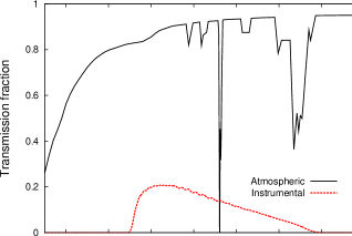
Spectral coverage: The wavelength range covered by the spectrograph needs to bracket a few significant spectral features. As shown in the bottom plot of Fig. 8, for our simulation the coverage is roughly from to , with decreasing sensitivity at longer wavelengths.
-
2.
Integration time: The faintest galaxies detectable by upcoming optical surveys can be a few orders of magnitude fainter than the atmospheric emission. Thus, significant integration times, as well as careful subtraction of the sky background, are needed to obtain secure redshift measurements.
-
3.
Cross-correlation templates: Having an accurate and representative set of galaxy spectral distribution templates is important in deriving accurate redshifts and associated uncertainties. As we discuss in the next section, this is particularly important for early-type galaxies and galaxies at (also known as the redshift desert) because of the lack of strong emission features in the spectrograph window.
2.2 Principal spectral features
The two main emission lines used in optical spectroscopy are the [OII] (singly-ionized oxygen) line at and the (first transition in the Balmer series) line at . The main absorption feature is the break, caused by a confluence of absorption lines, particularly the H and K Calcium lines. In high-resolution spectroscopy, [OII] is the most important line because it is actually a doublet – a pair of closely spaced lines. High-resolution observations - e.g. with DEEP2 (Newman et al., 2012), or SDSS (York et al., 2000) - can distinguish the doublet and hence confidently identify [OII]. Low-resolution observations - e.g. as in the VVDS (Le Fèvre et al., 2005) and zCOSMOS surveys (Lilly et al., 2007), rely on more than one feature. The limited spectral range of the instrument sets the regions of redshift space where one can confidently identify spectral features. In the case of VVDS, for example, there are roughly 5 different redshift regions:
-
•
: The can be detected, but [OII] cannot. There is risk of confusing of a galaxy for [OII] emission of a galaxy at . Fortunately, these galaxies are mostly brighter and thus the line combined with less prominent spectral features is often sufficient to estimate a redshift. Similarly, for early type galaxies, the break cannot be detected, and one relies on smaller absorption features.
-
•
: Neither [OII] nor can be detected. Redshifts have to be estimated based on [OIII] and lines.
-
•
: [OII] and other important lines ([OIII] - , - ) are detectable, but get progressively fainter towards higher redshift (due to increasing atmospheric noise and instrumental sensitivity).
-
•
: [OIII] and are out of the instrument range, but [OII] and the break are still detectable.
-
•
(the redshift desert): Only minor features in the spectra are available. Visual inspection to reduce incompleteness is essential in this range. Potential for wrong redshifts is increased because atmospheric emission lines can be mistakenly identified by the algorithm as real lines.
2.3 Additional systematics affecting the incompleteness
There are a few additional items contributing to the incompleteness of spectroscopic surveys that are not modeled in our simulations but that exist in real surveys:
-
•
Fiber collisions and slit overlaps: If the angular separation between galaxies is too small, one may not simultaneously obtain their spectra (without using a multiple pass strategy). Since clustering of galaxies is type dependent, one has to be careful that fiber collisions and slit overlaps do not introduce selection biases.
-
•
Optical distortions: Geometric distortions due to the spectrograph optics may make extraction of spectra and subsequent measurement of redshifts more difficult near the edge of the instrument field of view.
-
•
CCD fringing: Spatial and wavelength dependent variations in the pixel response in the red end of the spectrograph. Fringing hinders measurement of the spectra and redshifts of faint galaxies.
-
•
Stars and bright galaxies: Light from nearby stars or bright galaxies can contaminate the spectra.
-
•
Cosmic rays: Also can contaminate the spectra.
Issues such as stars, cosmic rays and edge effects will reduce the completeness, more or less randomly, resulting mostly in an increase in the shot noise, without galaxy type or redshift dependence. Note also, that photometric surveys are affected by countless other selection systematics. We are only concerned with systematic differences between the spectroscopic sample relative to the photometric sample, however it is defined.
3 Simulated Data
We use cosmological simulations populated with galaxies and their photometric properties as described in Appendix A.1. The photometric observations are patterned after the expected sensitivity of the Dark Energy Survey (DES) and Vista Hemisphere Surveys (VHS), with galaxies imaged in the grizYJHKs filters over 5100 sq. degrees. For simplicity, we only use the observations on griz bands because they are imaged for longer periods of time, and hence are useful for all our sample. The imaging in these bands is expected to reach magnitude limits of 25.2, 24.7, 24.0, and 23.5 in g,r,i and z.
For computational efficiency, we select a subsample of approximately 1.3 million galaxies, hereafter our photometric sample, from the total 1 billion galaxies present in the simulation. We apply the same quality cuts as in Cunha et al. (2012), i.e. keep galaxies with and at least detection in grz. This selection reduces our photometric sample to 726824 galaxies.
Of this photometric sample, we randomly target a subset of 181892 galaxies, hereafter the spectroscopic sample or training set, for the spectroscopic analysis. The generation of simulated spectra for this subsample is described in the Appendix A.2.
4 From the redshifts to cosmology
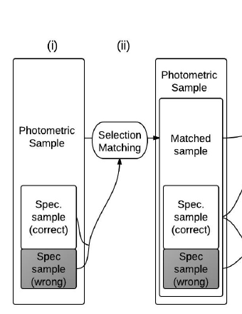
In this section, we describe the step-by-step procedure we used for converting the simulated observations into cosmological constraints. The flowchart in Fig. 1 gives a pictorial version of the explanation below.
-
1.
The first step is to estimate spectroscopic redshifts for the sample for which we have spectra. We use the rvsao.xcsao spectral analyzer algorithm described in Sec. 4.1. Not all spectra yield redshifts, and only the redshifts above certain confidence are kept. Even so, a fraction of the spectroscopic redshifts is incorrect.
-
2.
The spectroscopic sample can only be used for calibration of the photo-z error distributions if it is a representative subsample of the photometric sample. Hence, we statistically match spectroscopic and photometric selection in one of two ways: by applying the spectroscopic selection to the photometric sample with neural networks (cf. Sec. 6.1), or by weighting the photometric sample so that its statistical properties match those of the spectroscopic sample (cf. Sec. 6.2).
-
3.
Next, we calculate photo-zs for both the spectroscopic and photometric samples, cf. Sec. 4.2.
-
4.
After the matching, we can calculate the photo-z error matrices required for cosmological analysis.
-
5.
Finally, we estimate fiducial constraints and biases in the cosmological parameters forecasted for the DES-type weak gravitational lensing survey. We break up the tests in two parts. In the first case, shown as the transparent hexagon in the flowchart, we only test the impact of the selection matching, by using only the correct value for redshifts. In the second case (gray hexagon), we use the actual value of the spectroscopic redshifts - thereby including the small fraction of wrong redshifts.
4.1 Analyzing 1-D spectra
Simulating spectroscopic redshift estimation is challenging because real spectroscopic surveys rely heavily on visual inspection. For our forecasts, visual inspection of thousands of spectra would be out of the question. Instead, we adopt a more reasonable strategy and apply an automated pipeline to all 1-D spectra. We use the publicly available rvsao IRAF external package version 2.7.8 (Kurtz & Mink, 1998). We run the cross-correlation tool xcsao on our simulated spectra. The algorithm performs a Fourier cross-correlation between the “observed” (simulated) spectra and a user-defined library of template spectra. We obtain the template library used in the cross-correlation from the simulation itself. For the first pass, we pick 6 templates chosen to mimic the 6 galaxy templates used in the cross-correlation analysis of the SDSS spectroscopic pipeline111Templates 23 to 28 in the website: http://www.sdss.org/dr7/algorithms/spectemplates/index.html . Using templates from the simulation instead of the original SDSS templates improved the number of correct redshifts by . The limitation of the SDSS template basis is that it was chosen for low redshift spectroscopy, and is not sufficient for redshifts greater than 1 or so. In the second pass, we added three templates from the simulations picked as the brightest templates above redshift 1.4 for which the cross-correlation coefficient — the R statistic described below — was less than 2.5. The additional templates doubled the number of correct redshifts above 1.4.
The cross-correlation analysis can be refined around certain wavelengths by giving it an initial redshift guess (by setting the parameter czguess) to start the search. We perform the analysis five times with: no guess, czguess = 0.4, czguess = 0.8, czguess = 1.2 and czguess=1.6. We then choose which redshift estimate to keep based on the value of the R statistic, output by the pipeline. The R statistic, introduced by Tonry & Davis (1979) (cf. Eq. 23 of that work), is a measure of the strength of the cross-correlation given by the ratio of the height of the assumed true peak in the correlation to the average height of spurious peaks. R varies from 1 to several hundred in our simulation, and as we show later, corresponds to correct redshifts.
We have performed our analysis for a number of settings of the spectroscopic pipeline, but only show results for three main cases, defined as follows:
-
•
Fiducial Pipeline: s estimated using the 6+3=9 templates and the five redshift guesses described above. Yields the highest completeness for .
-
•
Comb2 Pipeline: s estimated using the 6+3=9 templates and only running xcsao twice, with czguess = 0.4 and czguess = 0.8. Yields the highest overall completeness, but the lowest completeness at low and high redshift.
-
•
Original Pipeline: s estimated using the 6 original templates and only four redshift guesses: czguess = none, 0.4, 0.8 and 1.2.
4.2 Photometric redshifts
There exists a cornucopia of publicly available photometric redshift estimation algorithms. For recent reviews and comparison of methods see e.g. Hildebrandt et al. (2010); Abdalla et al. (2011). We consider two different photo-z algorithms that broadly span the space of possibilities. We use a training-set fitting method with a very large training set and basic template-fitting code without any priors, which we briefly describe below.
4.2.1 Training-set redshift estimators
The basic setup of training-set based redshift estimators is to use a sample with known spectroscopic redshifts to estimate the free parameters of a function relating the observables (in our case the magnitudes of the galaxies) to the redshifts. After the best-fit free parameters have been determined, the function can be applied to the data for which no spectroscopic redshifts are available, known as the photometric sample. For this paper, we use an artificial neural network as our training set method, and we leave the details to Appendix B.
4.2.2 Template-fitting redshift estimators
Template-fitting estimators derive photometric redshift estimates by comparing the observed colors of galaxies to colors predicted from a library of galaxy spectral energy distributions. We use the publicly available LePhare photo-z code222http://www.cfht.hawaii.edu/~arnouts/LEPHARE/lephare.html (Arnouts et al., 1999; Ilbert et al., 2006) as our template-fitting estimator. We chose the extended template library, which comes with Lephare because it yielded the best photo-zs for our simulation. This library includes the four CWW templates (Coleman et al., 1980) extended to the IR and UV using templates from Bruzual & Charlot (2003) and six Kinney et al. (1996) starburst templates.
We note that a variety of public template-fitting codes are available (e.g. Coe et al., 2006; Feldmann et al., 2006), and each includes many options of template libraries, extinction laws, priors, etc. For a discussion on propagation of template-fitting uncertainties to redshift uncertainties see Abrahamse et al. (2011).
We emphasize that both categories of photo-z estimators should be thought of as performing the same function, of applying a model to describe the data. For training set methods, the model is the training sample, whereas for template-fitting methods, the model is the set of templates and priors utilised. By construction, the training-set method we use has an excellent training set, and as a result, performs nearly optimally. Conversely, for the template-fitting method, we do not take many pains to optimize the template library nor to find appropriate priors, and thus, the template-fitting code performs substantially worse. With perfect templates and perfect priors, template-fitting should equal the performance of training set methods with perfect training. It is not our intention to suggest that any of these estimators is fundamentally superior, we just wished to test our analysis in optimistic and pessimistic regimes. Most importantly, as we show in later Sections, results are independent of the photo-z estimators used despite the significant differences in performance.
4.3 Effect on the Cosmological Parameters
In Appendix C we review the formalism from BH10 to calculate the biases in the observed weak lensing power spectra, and hence in the cosmological parameters, given some arbitrary source systematic error. Here, we are of course interested in the systematics due to imperfect spectroscopic redshifts. It is beyond the scope of the paper to consider the biases for other cosmological probes, but we believe that the WL results will provide a useful baseline for what to expect from a single probe. In addition, we expect that a joint analysis might allow for self-calibration of the biases.
The fiducial weak lensing survey corresponds to expectations from the Dark Energy Survey, and assumes 5000 square degrees (corresponding to ) with tomographic measurements in uniformly wide redshift bins extending out to . The effective source galaxy density is 12 galaxies per square arcminute, while the maximum multipole considered in the convergence power spectrum is . The radial distribution of galaxies, required to determine tomographic normalized number densities in Eq. (6), is determined from the simulations and shown in Fig. 4.
We consider a standard set of six cosmological parameters with the following fiducial values: matter density relative to critical , equation of state parameter , physical baryon fraction , physical matter fraction (corresponding to the scaled Hubble constant ), spectral index , and amplitude of the matter power spectrum where (corresponding to ).
As detailed in Appendix C, we add the (unbiased) Planck forecasted constraints on the cosmological parameters to those of the DES. The fiducial (combined) constraint on the equation of state of dark energy assuming perfect knowledge of photometric redshifts is .
5 Spectroscopic success and failure
In this section we define the basic concepts regarding successful and failed galaxy spectra, and the accompanying rates.
5.1 Spectroscopic success rate
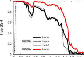
The spectroscopic analysis for the fiducial simulation parameters (16200 secs integration; 9 templates; no manual correction of spectra) yields about correct spectroscopic redshifts (defined as redshifts for which ). In a real survey, one can only choose redshifts based on some quality flag, which is the cross-correlation R statistic (described in Sec. 4.1) in our case. We thus define two success metrics:
-
•
True spectroscopic success rate (): the fraction of galaxies with correct redshifts.
-
•
Observed SSR (): the fraction of galaxies with R greater than a certain value. Unless stated otherwise, we set the value to 6.0.
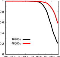
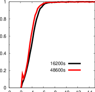
In Fig. 2, we show the true SSR as a function of true redshift (left panel), observed i-band magnitude (center panel) and cross-correlation strength (right panel). The left panel shows that the generally worsens with higher redshift, and the ’hiccups’ in the curves are directly caused by different spectral lines which enter and leave the observed spectral range, as discussed in Sec. 2. The central panel shows the expected result that the spectroscopic success rate plunges beyond certain depth. Finally, the right panel shows that the true SSR increases monotonically with cross-correlation statistic R, showing that we can use R to select an accurate redshift sample with high confidence.
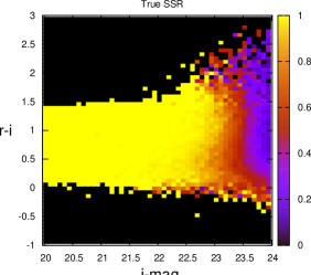
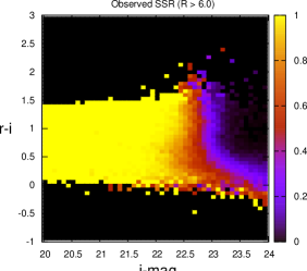
In Fig. 3 we show the true and observed SSRs as a function of -magnitude and – color. The top panel shows that virtually all the incorrect redshifts are at the faint end of the color-magnitude diagram, with slight color dependence. In particular, at the bluest end (–) we see a region of low SSR extending to . This is typically caused by the lack of an appropriate template to describe certain galaxy populations.
The observed SSR, shown in the bottom panel of Fig. 3, shows a more pronounced color variation. We can see that the bluer colors, corresponding to late spectral types, which have significant emission features, yields highest . Conversely, the redder colors have the lowest . As mentioned previously, early type galaxies have virtually no emission lines, and hence are identified by absorption features. Intermediate types can have weak emission lines, but usually have weaker absorption features as well, which makes it difficult to determine a spectroscopic redshift for them.
Because of our stringent choice of cut, the sample with contains a fraction 0.53 of the total galaxies and has correct spectroscopic redshifts. For comparison, if we define samples by the cuts and these would contain a fraction of 0.60 and 0.73 of total galaxies with and correct redshifts, respectively. Faint, intermediate-type galaxy spectra yield the majority of the incorrect redshifts that escape the R selection.
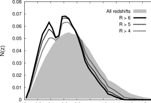
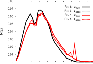
In the top panel of Fig. 4 we show the effect of applying quality cuts based on the statistic R to the true redshift distribution. More stringent (higher R) cuts preferentially remove galaxies from regions where less significant spectroscopic features fall inside the spectrograph window (as explained in Sec. 2). The bottom panel shows that the less stringent cuts allow for a higher fraction of incorrect redshifts, which have a visible impact in the redshift distribution even though of the redshifts are correct.
5.2 Where do the wrong redshifts go?
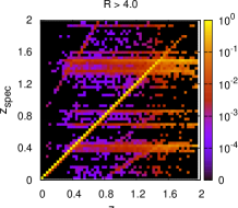
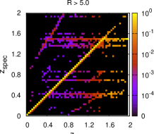
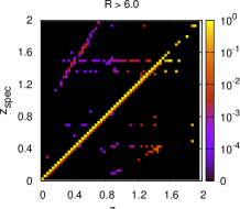
We show the spectroscopic leakage matrices () for several cuts in the R statistic for our Fiducial pipeline scenario in Fig. 5. The spectroscopic redshift errors, which correspond to any departures from the (diagonal) line, clearly make interesting and definite patterns:
-
•
Atmospheric line confusion: Horizontal features in Fig. 5, when many different values of are misinterpreted as a single , correspond to cases where residuals from subtraction of atmospheric lines are confused with actual features in the galaxy spectrum.
-
•
Galaxy line misidentification: Diagonal lines in Fig. 5 (excepting the diagonal, of course) correspond to the cases where the pipeline misidentifies lines of the galaxy itself due to limited spectroscopic coverage and S/N (cf. Sec. 2.2). For example, the diagonal trend from to about corresponds to the pipeline classifying H emission lines as [OII] lines. A corresponding feature due to [OII] being incorrectly classified as H can be seen starting at (0.8, 0) in the plots. Galaxy line misidentification seems to be a much smaller issue than atmospheric line confusion for our simulation.
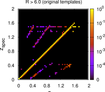
The exact distribution of the wrong redshifts depends on the noise levels assumed and details of the spectroscopic analysis. As described in Appendix A.2, we assumed a constant mean atmospheric emission and absorption, but in reality the observing conditions vary. The distribution of wrong redshifts also depends on details of the spectroscopic analysis. In Fig. 6 we show the matrix for the Original pipeline, described in Sec. 4.1, which only uses the original 6 spectral templates (but not the 3 templates added to increase completeness for .) In addition, it does not use the czguess=1.6 results, which have the effect of increasing the probability that the pipeline will assign a high redshift to a galaxy. The Original pipeline is not optimized in any way towards high-z completeness, and as a result it finds no spectroscopic redshifts above . Conversely, the Fiducial pipeline (cf. right plot in Fig. 5), does find some redshifts above , but at the cost of increasing the number of objects being incorrectly assigned very high values of spectroscopic redshifts and the number of objects at high redshifts being assigned very low redshifts. As we discuss in Sec. 6.1.2, the Original pipeline yields a bias in a factor of two smaller than the Fiducial pipeline.
There are two points to take from this section. First, wrong spectroscopic redshifts occupy preferred regions of the (, ) plane. Since the exact redshift error distribution depends on the details of the spectroscopic analysis and observing conditions, it is challenging to accurately predict the spectroscopic redshift errors in real surveys. Hence, our conclusions concerning the impact of wrong redshift are necessarily only rough estimates. Second, increasing the completeness at high redshift can come at the expense of introducing more catastrophic spectroscopic redshifts. As we shall show in Sec. 6.1.2, this is a very high price to pay, and can severely increase biases in cosmological parameter constraints.
6 Spectroscopic selection matching
As can be inferred from the top panel in Fig. 4, spectroscopic failures alter the redshift distribution of the training set significantly, so that one cannot use such a sample to estimate the error distributions of the photometric sample directly. We test two different approaches to correct for the selection effects in the training set.
One approach, presented in Sec. 6.1 is to cull the photometric sample to remove all galaxies that are not represented in the training set (the set of high-confidence spectroscopic redshift galaxies). The other approach, described in Sec. 6.2 is to apply weights to the spectroscopic sample so that the statistical properties of the weighted spectroscopic galaxies closely match those of the photometric sample. Thus, in the first approach, the photometric sample is modified to match the spectroscopic sample, whereas in the second approach, it is the spectroscopic sample that is modified.
6.1 Culling approach to selection matching
In the culling approach, we use a neural network (described in Appendix B) to accomplish the selection matching. What we want is to be able to classify galaxies in the photometric sample in the same way they were classified in the training set, that is, we need to estimate the cross-correlation strength R statistic for them.
To be more realistic, instead of using R, we map the R values into a new quality parameter Q. The Q parameter is discrete, and roughly matches the more standard quality flags of real surveys (e.g. VVDS, DEEP2). It also has the advantage of having a more limited range than the R statistic, which has no upper limit. The mapping we use is as follows:
The relationship between and Q classification depends slightly on the exposure time, but can be inferred from the right plot of Fig. 2.
Following standard neural network procedure, we split the spectroscopic sample into two parts (of equal size), the training and validation samples. As described in Appendix B, we use the magnitudes as the inputs for the neural network, which then outputs an estimate for . For simplicity, we only perform a single neural net run, though the average of multiple runs is expected to yield best results.
After the neural net run converges, we apply the best-fit function to the complete spectroscopic sample and to the photometric sample to obtain estimates of the Q coefficient, hereafter , for all the galaxies. Note that is continuous, whereas Q is discrete.
The matching between Q and is very good for the galaxies. For the 16200 sec exposures, the width of the distribution is 0.05, and only of the galaxies with have . The matching is less accurate for the galaxies for the lower Q, with the worst case being the sample, for which . Interestingly, the redshift success statistics for the Q-selected sample are very similar to those of a selected sample. Most importantly, the spectroscopic success rate increases monotonically with (not shown), making it an accurate classifier of redshift confidence. We leave more detailed comparisons between Q and for future work.
We apply cuts on , 2.5, and 3.5 to both spectroscopic and photometric samples. With the 16200 sec exposures, the corresponding True SSR for the galaxy samples is 0.996, 0.978 and 0.914, respectively, with a corresponding fraction of objects relative to the total of 0.463, 0.586 and 0.751 in the three cases. For the 48600 sec exposures, we find True SSRs of 0.996, 0,978 and 0.936 respectively, with corresponding fractions of objects retained of 0.655, 0.808 and 0.960.
The next step is to investigate the impact of the selection to the weak lensing analysis. We break up the process into several parts, for clarity:
-
•
If a training set based method is to be used for calculating photo-zs, the first step is to use the training sample with the desired cut to derive photometric redshifts for the matched photometric sample (cf. Sec. 6.1.1). This step may be skipped if a pure template-based algorithm is being used.
-
•
Next, we calculate the WL constraints for the photometric sample selected with the cut and compare that to what we get for the full sample. Constraints degrade both from the reduction in the total number of objects as well as with the shift of the redshift distribution towards lower redshifts (cf. Sec. 6.1.2).
-
•
The next step is to assess the bias resulting from differences in the selection of the spectroscopic and photometric samples as well as the biases due to wrong redshifts. (cf. Sec. 6.1.2).
6.1.1 Photo-z training
We use a neural network photo-z estimator to exemplify the impact of selection matching and wrong redshifts on training-set based photo-z estimation (cf. Sec. 4.2.1). For simplicity, we assume that the photo-zs for the photometric sample should only be calculated for the subset of galaxies surviving the selection cuts of the previous section. In other words, we require that the spectroscopic training sample and the photometric sample have matching selections. We thus define three sets of spectroscopic and photometric samples, specified by the spectroscopic quality cuts on of 3.5, 2.5, or 1.5.
To separate the effects of selection matching from the effect of wrong redshifts, we estimate the photo-zs twice. First, we assume we have the true redshifts for all galaxies passing the cuts, to isolate potential biases due to the spectroscopic selection matching. Then, we perform the photo-z training on the actual spectroscopic redshifts, to gauge the additional impact of wrong redshifts.
Table 1 shows the photo-z scatter for the samples defined by the cuts. The two columns correspond to the scenarios where the true redshifts were used in the training. The scatter is defined as the dispersion in the distribution of for both the training sample and photometric sample. As expected, the photo-z scatter of the training sample is in excellent agreement with the scatter of the photometric sample, suggesting that both samples have close to identical photo-z properties and that the selection matching does not introduce any biases. Furthermore, the scatter improves as we apply more stringent cuts on . The decrease in scatter is as expected, since the objects with low are typically the faintest.
The three columns in Table 1 show the more realistic case where the actual spectroscopic redshifts (wrong redshifts included) was used to train the photo-zs. In the we show the scatter in the training set calculated as the dispersion in the distribution, which we can see is in excellent agreement with the scatter of the photometric sample shown in the fifth column. Comparing the dispersion of the and cases, we see that the presence of wrong redshifts degrades the photo-zs of the photometric sample by as much as in the case of the cut. The degradation is reduced for the more stringent cuts as the fraction of wrong redshifts is reduced.
In reality, one does not know the true redshifts for the training set, but only the spectroscopic redshifts. Hence, the scatter in the training set photo-zs would be estimated using the spectroscopic redshifts, as the dispersion in the distribution. We show this estimate of the scatter in the column. We see substantially larger values of the scatter compared to the column, for all cuts. The point is that the neural network is not substantially affected by the wrong redshifts, so that the true scatter does not degrade. However, our estimate of the scatter using the spectroscopic redshifts is strongly affected, as the wrong spectroscopic redshifts show up as catastrophically incorrect redshifts, which we can often remove.
We therefore conclude that the use of training samples is still justified in the presence of incorrect redshifts. For the sake of comparison, the template-fitting photo-zs without any priors have rms scatter of 0.229, 0.215 and 0.203 for the samples selected with , 2.5 and 3.5, respectively. If the scatter were estimated using the spectroscopic redshifts, then the rms would be 0.313, 0,246 and 0.211 for the same cases. A more careful analysis of the template-fitting photo-zs could certainly produce better results. However, as we show in the next Section, the cosmological biases are very similar whether template or neural net photo-zs are used, and we leave more detailed analyses for future work. For more comparisons between these two methods using a catalog with similar photometry, see Cunha et al. (2012).
| Photo-z scatter and training set size | |||||
|---|---|---|---|---|---|
| Selection | Train | Photo | Train | Photo | Train* |
| 0.121 | 0.121 | 0.149 | 0.149 | 0.214 | |
| 0.098 | 0.099 | 0.105 | 0.106 | 0.142 | |
| 0.082 | 0.083 | 0.081 | 0.082 | 0.098 | |
6.1.2 WL constraints and biases
In this section we examine the constraints and biases in the dark energy equation of state inferred from weak lensing shear-shear correlations. The errors in are caused by our inability to characterize the photometric redshift error distribution of our sample. In other words, we must know the error matrix for our photometric sample to high accuracy. When we rely on a spectroscopic sample to characterize the error distribution, we are actually estimating , but this distribution differs from the true error matrix because of issues in spectroscopic selection matching and wrong spectroscopic redshifts. We now investigate how these spectroscopic redshift errors affect the dark energy equation of state measurements.
Table 2 shows the constraints on and systematic errors for several different sample selections. The results shown used template-fitting photo-zs described in Sec. 4.2.2. For clarity, we artificially separate the issues due to selection matching from that of the wrong redshifts as follows: we perform the cosmological parameter forecast analysis assuming that all redshifts that passed the selection cut were the correct, true redshifts, thereby explicitly isolating the selection matching systematics. The results are presented under the column in Table 2. We can see that biases in are negligible compared to the statistical constraints, demonstrating that the neural network can accurately match the spectroscopic selection to the photometric sample. The table also shows the fraction of galaxies surviving the selection cuts. For example, for the 16200 secs exposures, we see that the cut removes more than half of the sample, which results in nearly a factor of two degradation in the statistical constraints relative to what is achievable with the full sample (). The degradation is so severe because most of the objects removed by the cut are at high redshifts.
Next, we examine the impact of wrong redshifts. As the last column of Table 2 shows, wrong redshifts can be devastating to the weak lensing constraints. The bias in is, perhaps, tolerable only in the cases. In the other scenarios one can see that the biases in are greater than the constraints even with close to correct redshifts ().
Comparing the 48600 secs and 16200 secs results we see that the magnitude of the biases in are set entirely by the spectroscopic success rate (), regardless of the level of completeness. This is another reminder that the emphasis must be on accuracy over completeness.
| Constraints on (template-fitting photo-zs) | |||||
|---|---|---|---|---|---|
| 16200 secs | bias | ||||
| Selection | Gal. Frac. | () | |||
| 0.75 | 91.4 | 0.07 | 0.004 | - 0.52 | |
| 0.59 | 97.8 | 0.09 | 0.002 | - 0.13 | |
| 0.46 | 99.6 | 0.10 | -0.001 | - 0.02 | |
| 48600 secs | |||||
| 0.96 | 93.6 | 0.06 | 0.004 | - 0.39 | |
| 0.81 | 97.8 | 0.07 | 0.005 | - 0.15 | |
| 0.66 | 99.6 | 0.08 | 0.003 | - 0.03 | |
We investigated the dependence of the results on the photo-z estimator by performing the WL analysis with the neural network photo-zs instead of the template photo-zs. The resulting biases in are shown in the third column of Table 3. Comparing to the fourth column, where we reproduce the template photo-z biases from Table 2, we see that the magnitude of the bias is very similar for the two photo-z estimators, despite noticeable differences in the photo-z error distributions of both (see e.g. Cunha et al., 2012).
We also tested the possibility of decreasing the biases by culling photo-z outliers. In the presence of wrong spectroscopic redshifts, the culling could remove not only catastrophic photometric redshifts, but perhaps also identify the wrong s. We used the nearest-neighbor error estimator, NNE (Oyaizu et al., 2008a), to cull of the sample selected as the galaxies with largest NNE error, (). Since the fraction of objects to be culled was fixed, the value of the cut varied for each catalog and photo-z estimator. The results are presented in the last two columns of Table 3. For simplicity, we did not recalculate the fiducial constraints when deriving the biases for the culled samples; given the qualitative nature of this analysis, this is a reasonable approximation. The NNE cut seems quite effective for the neural network photo-zs, typically reducing the biases by half. When the NNE culling was applied to the template-fitting estimator, the effect was negligible for the case, and relatively small for the other cases, suggesting that the NNE is only effective for identifying spectroscopic outliers when a training set based procedure is used. This is by no means obvious since the NNE is very efficient at identifying photo-z outliers even when template-fitting methods are used (Oyaizu et al., 2008a). For comparison, we also tested the effect of applying the same cut using an error estimator from the template-fitting code itself333The error estimate we use is the difference between the Z_BEST68_HIGH and Z_BEST68_LOW outputs of the LePhare code. - shown in the last column of Table 3. We find that the biases due to wrong redshifts for the 1.5, 2.5 and 3.5 cases are reduced to -0.41, -0.086 and -0.014, showing that culling using this error estimator is also beneficial. We emphasize that the improvement from culling outliers is not due to the improvement of the photo-z statistics, but only due to the removal of spectroscopic failures with the culling. The effect on the neural net photo-zs was more significant simply because a larger fraction of failures was removed. In contrast, note that, in Cunha et al. (2012), we found that culling based on photo-z error estimates had little impact on cosmological biases due to sample variance in calibration sample, despite the effective identification of the photo-z outliers.
What about removing the wrong redshifts by comparing the photo-zs to spectroscopic redshifts? This is an intriguing option, but one must be very careful. The outlier islands of the photo-z error distribution often cause the largest biases in cosmological parameters (Bernstein & Huterer, 2010; Hearin et al., 2010). By removing catastrophic objects from the spectroscopic sample, one all but ensures that catastrophic islands will not be calibrated properly, thereby compromising the cosmological constraints. Hence, even though the comparison to photo-zs can produce a cleaner spectroscopic sample, its selection will no longer match that of the photometric sample. There are two ways to salvage the situation. Either one can apply the neural network procedure once again to match the selection, or one can directly remove the regions of observable space occupied by the objects with the corresponding photo-zs. The latter approach is essentially what we have done by performing the NNE cuts described in the previous paragraph. Regions of observable space for which the difference between and are large were removed from both the spectroscopic and photometric samples, thereby removing the spectroscopic outliers and simultaneously matching the corresponding selection in the photometric sample.
Finally, we investigated the dependence of the results on the details of our spectroscopic pipeline, described in Sec. 4.1. We find that our Fiducial pipeline, despite giving the best high redshift completeness, yielded the largest biases in , shown in the Table 2. The different pipelines yielded consistent trends, and we focus on one particular case, that highlights the importance of the settings. The Original pipeline had a factor of two smaller bias for the sample. In the Original setting, recall that only 6 templates were used. As can be seen by comparing the right plot in Fig. 5 with Fig. 6, the 3 additional templates increased the redshift completeness above but resulted in leakage from the high bins to low bins. In particular, some galaxies at were assigned s of and . This failure mode was responsible for about 2/3 of the increase in bias in going from the Original to the Fiducial pipeline. The remainder of the difference was due to the fact that the Fiducial pipeline uses which has the effect of increasing the probability that a galaxy will be assigned a high redshift. As a result, the Fiducial pipeline yields s above 1.5 for several galaxies with .
We conclude that the commonly adopted approach of maximizing the completeness is not recommended because it leads to the increase of the fraction of wrong redshifts which in turn implies worse dark energy parameter biases.
| Biases in (culling catastrophics with NNE ) | ||||||
|---|---|---|---|---|---|---|
| 16200 secs | No NNE Cut | NNE Cut | T. Cut | |||
| Selection | G. Frac. | neural | templ. | neural | templ. | templ. |
| 0.75 | - 0.27 | - 0.52 | - 0.19 | - 0.35 | -0.41 | |
| 0.59 | - 0.13 | - 0.13 | - 0.06 | - 0.11 | -0.09 | |
| 0.46 | - 0.02 | - 0.02 | - 0.01 | - 0.02 | -0.01 | |
6.2 Weights approach to selection matching
In Section 6.1, we matched the selection of the spectroscopic and photometric samples by culling the photometric sample. That is, we selectively removed galaxies from the photometric sample so that it statistically matched, as closely as possible, the spectroscopic sample. In this section we try a more aggressive approach that allows us to keep nearly the full photometric sample. Our technique is to weight galaxies in the spectroscopic sample using the probwts method of Lima et al. (2008) and Cunha et al. (2009), so that the statistical properties of these weighted spectroscopic galaxies match those of the photometric sample. For convenience of reference, we briefly describe the probwts technique in Appendix D.
We select a training set by picking galaxies from the spectroscopic sample with Q above some threshold . We test the reconstruction for several values of . Following standard probwts procedure, we remove the (small) part of the photometric sample that is determined to have zero overlap with the spectroscopic sample. This removes at most a few percent of the photometric sample, with negligible impact on the statistical constraints.
Note that, in the first approach, with the neural net, all the spectroscopic sample is used to characterize the spectroscopic selection in observable space. The cosmological analysis is then only performed on the sample that matches the estimated selection. In the second, we only use reliable spectra, which we re-weight to match the full photometric sample. Then, the full photometric sample is used on the cosmological analysis. The first approach is the more conservative one as it throws away photometric data, to keep only the most reliable sample. The second approach is more aggressive as it tries to keep most of the data and only rescale the training set.
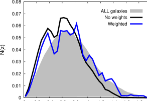
As the top plot of Fig. 7 shows, the weights improve the estimate of the overall redshift distribution when true redshifts are used. One can see that the weights roughly fix the broadest discrepancies, but cannot correct sharper features. For example, the dip in the training sample from around gets rescaled, but its rough shape persists. What this suggests is that objects in this redshift range occupied the same region of observable space, and the weighting affected them all similarly.
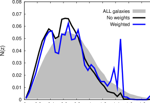
The bottom plot shows the results when the spectroscopic redshifts are used. We see that even a speck of wrong redshifts ( in this case) can have dramatic impact depending on where they are located (cf. bottom plot). Comparing, the bottom plot of Fig. 7 with the middle plot of Fig. 5, we see that the spikes in the Weighted estimated of the redshift distribution at 1.5, 1.4, 0.8, 0.7 and 0.4 all correspond to the regions of concentration of wrong redshifts seen in Fig. 5. However, whereas the spikes below are not particularly prominent, the spikes around and 1.5 are enormous. There are a couple factors contributing to the problem. As can be inferred from the the left plot in Fig. 2, the completeness drops precipitously above . Hence, the few spectroscopic redshifts above typically receive large weights to compensate for the incompleteness. In addition, as shown in the middle plot of Fig. 5, the fraction of correct redshifts for galaxies with is very small, and many of these are incorrectly assigned a spectroscopic redshift of or 1.5. The large weights magnify the impact of the wrong redshifts, resulting in the large spikes, and in large bias in the cosmological parameters, as we show in the next section.
6.2.1 Weak lensing constraints and biases with weights
Table 4 shows the constraints and biases on when one uses the weights technique to match the spectroscopic selection to the photometric sample. As in Sec. 6.1.2, we separate the analysis into two parts. First, in the column, we show only the effect of matching the selection between the spectroscopic and photometric samples. Afterwards, in the column, we use the actual spectroscopic redshifts to show the impact of wrong redshifts.
As shown in the Table the weights perform reasonably for all cases when one considers only the true redshifts. The biases are typically smaller than the statistical errors on , and the statistical constraints are better than for the culling approach of Sec. 6.1.2 since almost all of the photometric sample was usable for analysis. It is interesting to note that more rigorous cuts ( and 5) yielded the smallest biases even though the completeness of the spectroscopic sample was smaller than for the case. It is instructive to re-examine the top plot of Fig. 7. Comparing the blue solid line with the shaded gray region, we see that the weights reconstruction of the overall redshift distribution is quite jagged, yet it yields small biases in w. The reason for this is that the w is sensitive to a very broad redshift range, and an estimator can over- or under-estimate the overall redshift distribution in small redshift ranges as long as there are no net biases. This point is explored in much more detailed in Sec. 5.3.1 of Cunha et al. (2012). Unfortunately, the column in Table 4 shows that the presence of wrong redshifts severely compromises the weights approach.
Because the wrong redshifts are tightly associated with the regions of high incompleteness, particularly at high redshift, and because the variations in completeness are so sharp, the wrong redshifts received very large weights resulting in large cosmological biases. A major part of the problem is the sharp change in completeness with redshift shown on the left plot of Fig. 2. We find that the results for the weights do not improve for the 48600 secs cases because the steep variations in the completeness with redshift become even larger for that case since the increased exposure time did not yield significant increase in completeness above of 1.4.
In summary, we find that the weights approach needs to be considered with care in the presence of wrong redshifts, and that the more conservative approach of culling using the neural network is the safest. In practice, the weights are often needed to account for other types of incompleteness (see e.g. Cunha et al., 2009), so both approaches should be used in tandem.
| Constraints on (template-fitting photo-zs and weights) | |||||
|---|---|---|---|---|---|
| 16200 secs | bias | ||||
| Selection | G. Frac. | () | |||
| 0.73 | 93.2 | 0.06 | 0.070 | - 0.7 | |
| 0.60 | 98.6 | 0.06 | 0.034 | - 0.5 | |
| 0.53 | 99.6 | 0.06 | -0.036 | - 0.3 | |
7 Discussion: Robustness of assumptions and results
We now discuss the dependence of our results on the key assumptions and numerical tools used in this work.
-
•
N-body/photometric simulations: The success rate statistics are affected by luminosity function and distribution of galaxy types in the simulation. However, the main conclusions of our paper, concerning selection matching and impact of wrong redshifts, should not be affected. We tested the selection matching for a variety of situations (several of which we do not show), including varying atmospheric noise models and spectrograph resolution. For all cases, the matching worked well, incurring no additional bias. In addition, Soumagnac et al. (in preparation) obtain similar results using a very different set of spectro/photometric simulations described in Jouvel et al. (2009).
The distribution of wrong redshifts in space could also change for a different simulation, but the preferred loci where the failures concentrate should not vary appreciably, since they are based on confusion between galaxy or atmospheric spectral lines that do not depend on any details of the simulation. Furthermore, the fact that a small fraction of spectroscopic failures can cause severe biases is not likely to change.
-
•
Sky noise model: Our model for sky subtraction is idealized as it assumes a perfect shot-noise model. Sky-subtraction is often not as efficient, and observing conditions vary from the median. In addition, there are issues such as CCD fringing (cf. Sec. 2.3) which are difficult to model. Other effects we did not model include contamination from nearby stars or bright galaxies, and cosmic rays. These other effects, however, are only expected to affect the overall completeness, without galaxy type or redshift dependence.
-
•
Simulated spectra: As discussed in Appendix A.2, the simulated spectra we use are based on the 5 eigenspectra of kcorrect, which are derived based on about 1600 SDSS main sample galaxies, 400 luminous red galaxies and a photometric sample of several thousands of galaxies imaged in the UV, optical and IR. Is this enough? Yip et al. (2004) showed that a set of 3 eigentemplates were sufficient to describe about of the variance in the 170,000 galaxies in the Strauss et al. (2002) SDSS sample. Additional templates improved coverage very slowly, with a set of 500 eigentemplates needed to account for of the sample variance (cf. Table 1 in that work). Yip et al. (2004) show that the missing variance was due mainly to extreme line-emission galaxies. We roughly confirm this trend for our simulated spectra by looking at the distribution of equivalent widths of the [OII] emission line for our simulated galaxies. We find that our equivalent widths reach at most 30 . For comparison, Cooper et al. (2006) find, for the DEEP2 sample, a distribution of [OII] equivalent widths reaching as much as 100 .
In addition, Yip et al. (2004) showed that one needs a random subsample of about 10,000 galaxies to obtain convergence for the first 10 eigentemplates. These results suggest the kcorrect basis should be sufficient to characterize all but a few percent of the low-redshift galaxies444The Yip et al. (2004) analysis was based on principal component analysis, whereas Blanton & Roweis (2007) used non-negative matrix factorization to determine their respective eigenbasis. Thus, comparison between Blanton & Roweis (2007) and Yip et al. (2004) are only meant as ballpark estimates.. However, a few percent of “oddball” galaxies could potentially cause problems for cosmological analysis if they cannot be disentangled from the rest of the sample using colors and if their redshift distribution differs significantly from the rest of the sample with similar colors. The problem is expected to become worse at high-redshift. To properly quantify the impact of the outliers, observing campaigns targeted at the spectroscopic failures of existing spectroscopic surveys are crucial.
In some sense, our choice of template library used for deriving spectroscopic redshifts is pessimistic for the high-redshift galaxies: as discussed in Appendix A.2, the kcorrect templates are based on GALEX colors for the bluer frequencies. Hence, parts of the spectra of high-z objects were simulated using purely photometric data, resulting in excessively featureless spectra in the UV frequencies, which implied lower-than-expected completeness for .
-
•
Spectroscopic redshift pipeline The rvsao.xcsao code uses cross-correlation techniques in Fourier space to derive redshifts from spectra. The disadvantage of this approach relative to a standard method is that one does not include any information about the noise. One can disregard certain regions of the spectrum in the analysis, thereby removing at least the most prominent atmospheric lines. We found that the removal of some lines did not increase the completeness of the sample noticeably, and changed the distribution of the wrong redshifts. We leave more extensive tests on the optimal techniques for spectroscopic redshift estimation for a future work.
-
•
Culling approach to selection matching In a real spectroscopic survey, the success of the neural network culling approach to selection matching is likely to require a more careful redshift confidence classification. In our simulation, the atmospheric conditions were fixed for the full sample, and the noise subtraction was perfect. In a real survey, the variability of observing conditions and other problems such as slit placement and cosmic ray contamination will complicate the mapping between magnitudes in the photometric surveys and the redshift confidence in the spectroscopic survey. This difficulty can likely be overcome if some measure of the observing conditions is used as input when training the neural network. We leave these investigations for a future work.
8 Implications for Survey Design
Given the findings of this paper and Cunha et al. (2012), what should survey planners do to optimize their spectroscopic surveys?
The first step is obvious: one needs to optimize the allocation of time observing different kinds of galaxies. Specifically, one can use color information to preselect galaxies that will require longer exposure times to obtain accurate redshifts. For example, in Sec. 6.1.2, we saw that tripling the exposure time improved the completeness from 0.46 to 0.66 for the cut. If the of the sample that yielded additional redshifts could be known in advance, one would only target this sample for additional observation, which would only require an increase of in the observing time, instead of the naive additional time if the full sample was targeted for follow-up observation. With an optimized observing strategy, one would be able to save precious telescope time and still achieve redshift accuracy that does not degrade the cosmological constraints appreciably. We leave a more detailed analysis for future work.
We showed in this paper that the tolerance for wrong redshifts is extremely low. It is, however, possible to get away with a higher fraction of wrong spectroscopic redshifts by modeling their effects on the cosmological parameters. Then one would need to, in analogy to the photo-z case, fully characterize the spectroscopic error matrix . However, determining the matrix from observations is likely to be very challenging in practice, as in order to control the sample variance of galaxies used for the calibration, one would likely have excessively high requirements on the area of the follow-up (Cunha et al., 2012).
It is also possible that one can use spatial cross-correlations to estimate the spectroscopic error matrix. Since correlations between different redshift bins should be very close to zero, any correlation has to be due to wrong redshifts. Several works have explored this fact for photo-z calibration (Schneider et al., 2006; Erben et al., 2009; Benjamin et al., 2010; Zhang et al., 2010). Schneider et al. (2006), for example, found cross-correlations to work well only in the simplest Gaussian cases. But for spectroscopic failures, the excess correlation signal should be due to a few big outliers, and hence might be more easily detectable.
9 Conclusions
We investigated the impact of spectroscopic failures on the training and calibration of photometric redshifts, and the consequent impact on the forecasted dark energy parameter constraints from weak gravitational lensing. Our tests were based on N-body/spectrophotometric simulations patterned after the DES and expected spectroscopic follow-up observations loosely patterned after the VVDS survey.
Spectroscopic failures consist of two types of issues: the inability to obtain spectroscopic redshifts for certain galaxies, and incorrect redshifts.
The inability to obtain redshifts introduces incompleteness in the spectroscopic sample — i.e. missing redshifts in some region of parameter space (e.g. at faint magnitudes) represented in the full photometric population of galaxies. This incompleteness must be accounted for before one can use the spectroscopic sample to calibrate photo-zs – i.e characterize the photo-z error matrices, e.g. the , of the sample.
We studied two approaches to account for the incompleteness in the spectroscopic sample. In the first approach, we used an artificial neural network to estimate the spectroscopic selection function for the photometric sample. This selection function was then used to cull the photometric sample so that its statistical properties matched the spectroscopic sample. We found this approach works extremely well, yielding only insignificant bias in the WL constraints using the culled sample (refer to column in Table 2). However, the statistical constraints did degrade substantially as, typically, a large fraction of the sample was culled. In the second approach, we accounted for the incompleteness in the spectroscopic sample by applying weights to the galaxies with spectroscopic redshifts, following the approach of Lima et al. (2008), so that the statistical properties of the spectroscopic and photometric samples match. This approach was also successful (cf. column in Table 4) — as expected, because most of the photometric sample could be used — yielding tolerable cosmological biases while obtaining the maximum statistical constraints. Overall, we found that the effects of spectroscopic incompleteness are well under control.
Unfortunately, on the other hand, we found that wrong redshifts can significantly degrade cosmological constraints and of correct spectroscopic redshifts seems to be needed (cf. and columns in Tables 2 and 4). We found the results to be independent of the photo-z estimators used, but somewhat dependent on the settings of the spectroscopic pipeline. In particular, we found that attempts to increase the completeness of the spectroscopic sample during the spectral analysis can result in more catastrophic spectroscopic redshift failures, which will increase cosmological biases.
We tested a couple of approaches to identify wrong spectroscopic redshifts, finding that the NNE error estimator (Oyaizu et al., 2008a) is able to reduce the bias in the measured dark energy equation of state by half while removing only of the photometric sample. Slightly less improvement in the bias was obtained using the template-fitting error estimator.
In summary, we find that wrong redshifts are by far the main issue affecting calibration of photo-z error distributions with spectroscopic samples. Future follow-up spectroscopic observations of the planned and ongoing wide-area photometric surveys must focus primarily on the accuracy of the spectroscopic redshifts even if that implies sacrificing the spectroscopic completeness.
Acknowledgments
CEC would like to thank Joerg Dietrich, Stephanie Jouvel, Anja von der Linden, Jeff Newman and Peter Norberg for discussions about spectroscopic surveys. We also thank G. Bernstein, J. Cohn, and S. Lilly for detailed comments on the draft. This paper has gone through internal review by the DES collaboration. CEC is supported by a Kavli Fellowship at Stanford University. DH is supported by the DOE OJI grant under contract DE-FG02-95ER40899. DH is additionally supported by NSF under contract AST-0807564, and NASA under contract NNX09AC89G. RHW received support from the U.S. Department of Energy under contract number DE-AC02-76SF00515. MTB was supported by Stanford University and the Swiss National Science Foundation under contract 2000 124835/1. This research was supported in part by the National Science Foundation under Grant No. PHY05-51164, Grant No. 1066293 and the hospitality of the Aspen Center for Physics. Fermilab is operated by Fermi Research Alliance, LLC under Contract No. DE-AC02-07CH11359 with the United States Department of Energy.
Appendix A The simulations
In this section, we describe the construction of the simulations used in our analysis.
A.1 N-body/photometric simulations
The simulated galaxy catalog used for the present work was generated using the Adding Density Determined GAlaxies to Lightcone Simulations (ADDGALS) algorithm (Wechsler et al., 2011; Busha et al., 2011a). This algorithm attaches synthetic galaxies to dark matter particles in a lightcone output from a dark matter N-body simulation. The model is designed to match the luminosities, colors, and clustering properties of galaxies.
The simulations used here start with a dark matter lightcone which spans the redshift range from , over one octant of sky (5156 sq. degrees). The lightcone is constructed from three distinct N-body simulations, which range in resolution from a few to a few particles and box sizes ranging from 1 to 4 Gpc/. The simulations were run with the LGadget code and modeled a flat cosmology using parameters consistent with WMAP7 results.
The ADDGALS algorithm used to create the galaxy distribution consists of two steps: galaxies based on an input luminosity function are first assigned to particles in the simulated lightcone, after which multi-band photometry is added to each galaxy using a training set of observed galaxies. For the first step, we begin by defining the relation — the probability that a galaxy with magnitude a redshift resides in a region with local density , defined as the radius of a sphere containing of dark matter. This relation can be tuned to reproduce the luminosity-dependent galaxy 2-point function by using a much higher resolution simulation combined with the technique known as subhalo abundance matching. This is an algorithm for populating very high resolution dark matter simulations with galaxies based on halo and subhalo properties that accurately reproduces properties of the observed galaxy clustering (Conroy et al., 2006; Wetzel & White, 2010; Behroozi et al., 2010; Busha et al., 2011b). The relationship can be measured directly from the resulting catalog. Once this probability relation has been defined, galaxies are added to the simulation by integrating a (redshift dependent) -band luminosity function to generate a list of galaxies with magnitudes and redshifts, selecting a for each galaxy by drawing from the distribution, and attaching it to a simulated dark matter particle with the appropriate and redshift. The advantage of ADDGALS over other commonly used approaches based on the dark matter halos is the ability to produce significantly deeper catalogs using simulations of only modest size. When applied to the present simulation, we populate galaxies as dim as , compared with the completeness limit for a standard halo occupation (HOD) approach.
While the above algorithm accurately reproduces the distribution of satellite galaxies, central objects require explicit information about the mass of their host halos. Thus, for halos with more than 100 particles, we assign central galaxies using the explicit mass-luminosity relation determined from our calibration catalog. We also measure for each halo, which is used to draw a galaxy from the integrated luminosity function with the appropriate magnitude and density to place at the center.
For the galaxy assignment algorithm, we choose a luminosity function that is similar to the SDSS luminosity function as measured in Blanton et al. (2003), but evolves in such a way as to reproduce the higher redshift observations (e.g., SDSS-Stripe 82, AGES, GAMA, NDWFS and DEEP2). In particular, and are varied as a function of redshift in accordance with the recent results from GAMA (Loveday et al., 2012).
Once the galaxy positions have been assigned, photometric properties are added. We begin with a training set of spectroscopic galaxies and the simulated set of galaxies with -band magnitudes generated earlier. For each galaxy in both the training set and simulation we measure , the distance to the 5th nearest galaxy on the sky in a redshift bin. Each simulated galaxy is then assigned an SED based on drawing a random training-set galaxy with the appropriate magnitude and local density, k-correcting to the appropriate redshift, and projecting onto the desired filters. When doing the color assignment, the likelihood of assigning a red or a blue galaxy is smoothly varied as a function of redshift in order simultaneously reproduce the observed red fraction at low and high redshifts as observed in SDSS and DEEP2.
Differences between the training set and simulated galaxy sample complicate the process of color-assignment. In order to compile a sufficiently large training set, we use a magnitude-limited sample of SDSS spectroscopic galaxies brighter than with . The simulated sample, on the other hand, is a volume-limited sample, spanning a broader redshift range. When measuring we restrict ourselves to neighbors brighter than in the simulation sample, while using all objects in the observational catalog. To mitigate differences in luminosity and redshift, each galaxy is rank ordered according to its density in its redshift bin, and require that objects be in the same percentile bin in each sample rather than having the same the absolute value of . This is similar to the method used in Cooper et al. (2008).
The final step for producing a realistic simulated catalog is the application of photometric errors. While the photometric errors generated here are particular to DES, the algorithm can be generalized for any survey. For each galaxy, we add a noise term to the intrinsic galaxy flux, where the noise is drawn from a Gaussian of width
| (1) |
where is the exposure time, the number of pixels covered by a galaxy, the flux of the sky in a single detector pixel, and is the intrinsic flux of the galaxy. Here, galaxies are assumed to have the same angular size, hence is identical for all objects. Application of the above relation to objects from the SDSS catalog shows that it is able to faithfully reproduce the reported errors of the survey.
A.2 Creating simulated spectra
We use the kcorrect v4_1 code (Blanton et al., 2003) to derive simulated spectra. The kcorrect code includes a set of 5 eigenspectra derived using a non-negative matrix factorization (NMF) technique (Blanton & Roweis, 2007). To derive the eigenspectra, the authors start out with a basis of 450 star formation history templates from Bruzual & Charlot (2003) as well as 35 templates from Kewley et al. (2001). The method uses this basis to derive the nonnegative linear combination of templates that best described the observations. In this case, the observations consist of a sample of several thousand photometrically and/or spectroscopically observed galaxies, from the far UV to the near IR (Blanton & Roweis, 2007). The spectroscopic part of the training data consisted of 400 SDSS luminous red galaxies (LRGs) with (Eisenstein & other, 2001) and 1600 SDSS main sample galaxies with (Strauss et al., 2002), with both sets of data observed in the range .
We use the kcorrect subroutine to convert the true redshift and error-free magnitudes of a simulated galaxy from our photometric simulation into a best-fitting spectral energy distribution (SED). The SED is characterized by the coefficients of the 5 eigentemplates, and are output as the variable coeffs. The coeffs are then passed into the subroutine k_reconstruct_spec, which produces a simulated spectrum with a resolution, in units of velocity dispersion, of 300 km/s.
We pattern our mock survey loosely on the VIMOS-VLT Deep Survey (VVDS; Le Fèvre et al., 2005). The characteristics of the instrument that we assume are: collecting area of , aperture of . For simplicity, we assume a constant resolution and a dispersion of over the entire spectrograph range of . Comparing the spectrograph window of to the spectroscopic coverage of the training set used to create the simulated spectra, we see that for objects below redshift of 0.05, there is no spectroscopic representation of the training set galaxies in the range . More problematic is the fact that the spectroscopic training set has wavelength coverage starting at , and only goes to . As a result, for galaxies at about , the blue side of the simulated spectra are based solely on photometric data. Considering that most of the SDSS main sample is below redshift of 0.2, the simulated spectra should begin to lose resolution in the blue-end for . These limitations in the simulated spectra result in higher-than-expected incompleteness above , but do not affect the overall conclusions.
We use a Palomar sky extinction model (courtesy of B. Oke and J. Gunn) with 1.3 airmasses and altitude of 2635 meters to calculate the atmospheric transmission fraction (the solid black line in the bottom panel of Fig. 8). The instrument transmission is based on the VIMOS instrument transmission function555http://www.eso.org/observing/etc/bin/gen/form?INS.NAME=VIMOS+INS.MODE=SPECTRO and is shown as the dashed red line in the bottom panel of Fig. 8. The total transmission is the product of the atmospheric and instrumental transmissions. We assume 16200 secs exposures for the fiducial observation strategy and also investigate a scenario with 48600 secs exposures.
We add atmospheric emission based on the sky spectrum666Sky spectrum obtained from http://www.gemini.edu/sciops/ObsProcess/obsConstraints/atm-models/skybg\_50\_10.dat shown at the top panel of Fig. 8. The total noise is given by the rms sum of the atmospheric noise, shot-noise from the galaxy spectrum itself and readout noise per pixel, which we take to be a constant 5 photons. In reality, we only simulate the sky-subtracted spectrum, as follows. First, we convert the different spectra into photon counts for each pixel. We then assume the atmospheric and galaxy noise follow a Poisson distribution, so that the uncertainty in the produced noise is the square-root of the number of photons emitted. The readout noise is taken to be Gaussian. We calculate the total noise, as
| (2) |
where , , and are the number of photons from the atmosphere, the galaxy and the readout noise, respectively. The expected signal is simply the total number of photons from the galaxy. The expectation value of the error in the flux, is then given by
| (3) |
To obtain the sky-subtracted galaxy spectrum we, at each pixel, sample from a Gaussian distribution with mean given by the flux and width given by the error in the flux .

Appendix B Artificial Neural Networks
We use an Artificial Neural Network (ANN) method to both estimate the spectroscopic redshift quality and photometric redshifts, using an implementation based on (Collister & Lahav, 2004; Oyaizu et al., 2008b) Despite the fancy name, an ANN is simply a function which relates redshifts (or any quantity we wish to estimate) to photometric observables. The training set is used to determine the best-fit value for the free parameters of the ANN. The best-fit parameters are found by minimizing the overall scatter of the photo-zs determined for the training set galaxies. The ANN configurations are not unique in the sense that different sets of parameters can result in the same overall scatter. The best-fit parameters found after minimizing the scatter depend on where in parameter space the optimization run begins. Hereafter we refer to an ANN function using a given set of best-fit parameters as a neural network solution.
The technical details are as follows. We use a particular type of ANN called a Feed Forward Multilayer Perceptron (FFMP), which consists of several nodes arranged in layers through which signals propagate sequentially. The first layer, called the input layer, receives the input photometric observables (magnitudes, colors, etc.). The next layers, denoted hidden layers, propagate signals until the output layer, whose outputs are the desired quantities, in this case the photo-z estimate or the redshift quality Q estimate. Following the notation of Collister & Lahav (2004), we denote a network with layers and nodes in the layer as .
A given node can be specified by the layer it belongs to and the position it occupies in the layer. Consider a node in layer and position with . This node, denoted , receives a total input and fires an output given by
| (4) |
where is the activation function. The photometric observables are the inputs to the first layer nodes, which produce outputs . The outputs in layer are propagated to nodes in the next layer , denoted , with . The total input is a weighted sum of the outputs
| (5) |
where is the weight that connects nodes and . Iterating the process in layer , signals propagate from hidden layer to hidden layer until the output layer. In our implementation, we use a network configuration , which receives magnitudes and outputs a photo-z or a spectroscopic redshift quality. We use hyperbolic tangent activation functions in the hidden layers and a linear activation function for the output layer.
Appendix C Biases in weak lensing measurements of dark energy
To assess the impact of the spectroscopic failures on the cosmological parameters, we closely follow the formalism used in our previous work on the impact of sample variance to photo-z calibration (Cunha et al., 2012). We consider a weak lensing survey, and for simplicity only study the shear-shear correlations. The observable quantity we consider is the convergence power spectrum
| (6) |
where is the rms intrinsic ellipticity in each component, is the average number of galaxies in the th redshift bin per steradian, and is the multipole that corresponds to structures subtending the angle . For simplicity, we drop the superscripts below. We take .
We follow the formalism of Bernstein & Huterer (2010) (hereafter BH10), where the photometric redshift errors are algebraically propagated into the biases in the shear power spectra. These biases in the shear spectra can then be straightforwardly propagated into the biases in the cosmological parameters. We now review briefly this approach.
Let us assume a survey with the (true) distribution of source galaxies in redshift , divided into bins in redshift. Let us define the following terms
-
•
Leakage (or in BH10 terminology): fraction of objects from a given true redshift bin that are placed into an incorrect (non-corresponding) photometric bin.
-
•
Contamination (or in BH10 terminology): fraction of galaxies in a given photometric bin that come from a non-corresponding true-redshift bin.
When specified for each tomographic bin, these two quantities contain the same information. Note in particular that the two quantities satisfy the integrability conditions
| (7) | |||||
| (8) |
A fraction of galaxies in some true-redshift bin “leak” into some photo-z bin , so that is the fractional perturbation in the true-redshift bin, while the contamination is the fractional perturbation in the photometric bin. The two quantities can be related via
| (9) |
where and are the absolute galaxy numbers in the true and photometric redshift bins, respectively. Then,
| (10) | |||||
| (11) |
and the photometric bin normalized number density is affected (i.e. biased) by photo-z catastrophic errors. The effect on the cross power spectra is then
| (12) | |||||
(since the cross power spectra are symmetrical with respect to the interchange of indices, we only consider the biases in power spectra with ). Note that these equations are exact for a fixed contamination coefficient .
The bias in the observable power spectra is the rhs-lhs difference in the above equations777We have checked that the quadratic terms in are unimportant, but we include them in any case.. The cumulative result due to all contaminations in the survey (or, values for each and binned value) can be obtained by the appropriate sum
| (13) | |||||
for each pair of indices , where the second and third line assume and , respectively.
The bias in cosmological parameters is given by using the standard linearized formula (Knox et al., 1998; Huterer & Turner, 2001), summing over each pair of contaminations
| (14) |
where is the Fisher matrix and is the covariance of shear power spectra (see just below for definitions). This formula is accurate when the biases are ’small’, that is, when the biases in the cosmological parameters are much smaller than statistical errors in them, or . Here and label cosmological parameters, and and each denote a pair of tomographic bins, i.e. , where recall is the number of tomographic redshift bins. To connect to the notation in Eq. (12), for example, we have .
We calculate the Fisher matrix assuming perfect redshifts, and following the procedure used in many other papers (e.g. Huterer & Linder, 2007). The weak lensing Fisher matrix is then given by
| (15) |
where are the cosmological parameters and is the inverse of the covariance matrix between the observed power spectra whose elements are given by
where is the width of the binning in multipole . The survey specifications and the cosmological parameter set is described in Sec. 4.3. Finally, we add the information expected from the Planck survey given by the Planck Fisher matrix (W. Hu, private communication). The total Fisher matrix we use is thus
| (17) |
The fiducial constraint on the equation of state of dark energy assuming perfect knowledge of photometric redshifts is .
Our goal is to estimate the biases in the cosmological parameters due to imperfect knowledge of the photometric redshifts. In particular, the relevant photo-z error will be the difference between the inferred distribution for the calibration (or, training) set – using spectroscopic redshifts as a proxy for the true redshifts – and the distribution for the actual survey. Therefore, we define
| (18) | |||||
| (19) |
where the second line trivially follows given that the true, underlying power spectra are the same for the training and photometric galaxies. All of the shear power spectra biases can straightforwardly be evaluated from Eq. (13) by using the contamination coefficients for the training and photometric samples, respectively. Therefore, the effective error in the power spectra is equal to the difference in the biases of the training set (our estimates of the biases in the observable quantities) and the photometric set (the actual biases in the observables).
Appendix D Probwts
In this subsection, we briefly review the weighting method888The weights code is available at http://www.stanford.edu/~ccunha/nearest/. The codes can also be obtained in the git repository probwts at http://github.com of Lima et al. (2008) and Cunha et al. (2009). We define the weight, , of a galaxy in the spectroscopic training set as the normalized ratio of the density of galaxies in the photometric sample to the density of training-set galaxies around the given galaxy. These densities are calculated in a local neighborhood in the space of photometric observables, e.g. multi-band magnitudes. In this case, the DES griz magnitudes are our observables. The hypervolume used to estimate the density is set here to be the Euclidean distance of the galaxy to its nearest-neighbor in the training set. We set , to derive the most localized estimates possible.
The weights can be used to estimate the redshift distribution of the photometric sample using
| (20) |
where the weighted sum is over all galaxies in the training set. Lima et al. (2008) and Cunha et al. (2009) show that this provides a nearly unbiased estimate of the redshift distribution of the photometric sample, , provided the differences in the selection of the training and photometric samples are solely done in the observable quantities used to calculate the weights.
References
- Abdalla et al. (2011) Abdalla F.B., Banerji M., Lahav O., Rashkov V., 2011, Mon. Not. R. Astron. Soc., 417, 1891
- Abdalla et al. (2008) Abdalla F.B. et al., 2008, Mon. Not. Roy. Astron. Soc., 387, 969
- Abrahamse et al. (2011) Abrahamse A., Knox L., Schmidt S., Thorman P., Tyson J.A., Zhan H., 2011, Astrophys. J., 734, 36
- Amara & Refregier (2007) Amara A., Refregier A., 2007, Mon. Not. Roy. Astron. Soc., 381, 1018
- Arnouts et al. (1999) Arnouts S., Cristiani S., Moscardini L., Matarrese S., Lucchin F., Fontana A., Giallongo E., 1999, Mon. Not. R. Astron. Soc., 310, 540
- Behroozi et al. (2010) Behroozi P.S., Conroy C., Wechsler R.H., 2010, Astrophys. J., 717, 379
- Benjamin et al. (2010) Benjamin J., Van Waerbeke L., Menard B., Kilbinger M., 2010, Mon.Not.Roy.Astron.Soc., 408, 1168
- Bernstein & Huterer (2010) Bernstein G., Huterer D., 2010, Mon. Not. R. Astron. Soc., 401, 1399
- Blanton & Roweis (2007) Blanton M.R., Roweis S., 2007, Astro. Journal, 133, 734
- Blanton et al. (2003) Blanton M.R. et al., 2003, Astrophys. J., 592, 819
- Bordoloi et al. (2012) Bordoloi R., Lilly S., Amara A., Oesch P., Bardelli S. et al., 2012
- Bordoloi et al. (2010) Bordoloi R., Lilly S.J., Amara A., 2010, Mon. Not. R. Astron. Soc., 406, 881
- Bruzual & Charlot (2003) Bruzual G., Charlot S., 2003, Mon. Not. R. Astron. Soc., 344, 1000
- Busha et al. (2011a) Busha M., Wechsler R. et al., 2011a, in preparation
- Busha et al. (2011b) Busha M.T., Wechsler R.H., Behroozi P.S., Gerke B.F., Klypin A.A., Primack J.R., 2011b, ApJ, in press
- Coe et al. (2006) Coe D., Benítez N., Sánchez S.F., Jee M., Bouwens R., Ford H., 2006, Astro. Journal, 132, 926
- Coleman et al. (1980) Coleman G.D., Wu C.C., Weedman D.W., 1980, Astrophys. J. Supp., 43, 393
- Collister & Lahav (2004) Collister A.A., Lahav O., 2004, Proc. Astron. Soc. Pac., 116, 345
- Conroy et al. (2006) Conroy C., Wechsler R.H., Kravtsov A.V., 2006, Astrophys. J., 647, 201
- Cooper et al. (2008) Cooper M.C., Tremonti C.A., Newman J.A., Zabludoff A.I., 2008, Mon. Not. R. Astron. Soc., 390, 245
- Cooper et al. (2006) Cooper M.C. et al., 2006, Mon. Not. R. Astron. Soc., 370, 198
- Cunha et al. (2012) Cunha C.E., Huterer D., Busha M.T., Wechsler R.H., 2012, Mon. Not. R. Astron. Soc., 423, 909
- Cunha et al. (2009) Cunha C.E., Lima M., Oyaizu H., Frieman J., Lin H., 2009, Mon. Not. R. Astron. Soc., 396, 2379
- Eisenstein & other (2001) Eisenstein D.J., other, 2001, Astro. Journal, 122, 2267
- Erben et al. (2009) Erben T. et al., 2009, A&A, 493, 1197
- Feldmann et al. (2006) Feldmann R. et al., 2006, Mon. Not. R. Astron. Soc., 372, 565
- Hearin et al. (2010) Hearin A.P., Zentner A.R., Ma Z., Huterer D., 2010, Astrophys. J., 720, 1351
- Hildebrandt et al. (2010) Hildebrandt H. et al., 2010, A&A, 523, A31
- Huterer & Linder (2007) Huterer D., Linder E.V., 2007, Phys. Rev., D75, 023519
- Huterer et al. (2006) Huterer D., Takada M., Bernstein G., Jain B., 2006, Mon. Not. R. Astron. Soc., 366, 101
- Huterer & Turner (2001) Huterer D., Turner M.S., 2001, Phys. Rev., D64, 123527
- Ilbert et al. (2006) Ilbert O. et al., 2006, A&A, 457, 841
- Jouvel et al. (2009) Jouvel S. et al., 2009, A&A, 504, 359
- Kewley et al. (2001) Kewley L.J., Dopita M.A., Sutherland R.S., Heisler C.A., Trevena J., 2001, Astrophys. J., 556, 121
- Kinney et al. (1996) Kinney A.L., Calzetti D., Bohlin R.C., McQuade K., Storchi-Bergmann T., Schmitt H.R., 1996, Astrophys. J., 467, 38
- Kitching et al. (2008) Kitching T.D., Taylor A.N., Heavens A.F., 2008, Mon. Not. Roy. Astron. Soc., 389
- Knox et al. (1998) Knox L., Scoccimarro R., Dodelson S., 1998, Phys. Rev. Lett., 81, 2004
- Kurtz & Mink (1998) Kurtz M.J., Mink D.J., 1998, Proc. Astron. Soc. Pac., 110, 934
- Le Fèvre et al. (2005) Le Fèvre O. et al., 2005, A&A, 439, 845
- Lilly et al. (2007) Lilly S.J. et al., 2007, Astrophys. J. Supp., 172, 70
- Lima et al. (2008) Lima M., Cunha C.E., Oyaizu H., Frieman J., Lin H., Sheldon E.S., 2008, Mon. Not. R. Astron. Soc., 390, 118
- Loveday et al. (2012) Loveday J. et al., 2012, Mon. Not. R. Astron. Soc., 420, 1239
- Ma & Bernstein (2008) Ma Z., Bernstein G., 2008, Astrophys. J., 682, 39
- Ma et al. (2006) Ma Z., Hu W., Huterer D., 2006, Astrophys. J., 636, 21
- Nakajima et al. (2012) Nakajima R., Mandelbaum R., Seljak U., Cohn J.D., Reyes R., Cool R., 2012, Mon. Not. R. Astron. Soc., 420, 3240
- Newman et al. (2012) Newman J.A. et al., 2012, preprint (arXiv:1203.3192)
- Oyaizu et al. (2008a) Oyaizu H., Lima M., Cunha C.E., Lin H., Frieman J., 2008a, Astrophys. J., 689, 709
- Oyaizu et al. (2008b) Oyaizu H., Lima M., Cunha C.E., Lin H., Frieman J., Sheldon E.S., 2008b, Astrophys. J., 674, 768
- Schneider et al. (2006) Schneider M., Knox L., Zhan H., Connolly A., 2006, Astrophys. J., 651, 14
- Strauss et al. (2002) Strauss M.A. et al., 2002, Astro. Journal, 124, 1810
- Tonry & Davis (1979) Tonry J., Davis M., 1979, Astro. Journal, 84, 1511
- Wechsler et al. (2011) Wechsler R.H., T. B.M. et al., 2011, in preparation
- Wetzel & White (2010) Wetzel A.R., White M., 2010, Mon. Not. R. Astron. Soc., 403, 1072
- Yip et al. (2004) Yip C.W. et al., 2004, Astro. Journal, 128, 585
- York et al. (2000) York D.G. et al., 2000, Astro. Journal, 120, 1579
- Zhang et al. (2010) Zhang P., Pen U.L., Bernstein G., 2010, Mon. Not. R. Astron. Soc., 405, 359