arXiv:1207.3335

UT-Komaba/12-6


Gauge-invariant observables and marginal deformations

in open string field theory

Matěj Kudrna,1 Toru Masuda,2 Yuji Okawa,2 Martin Schnabl1 and Kenichiro Yoshida3
1Institute of Physics AS CR
Na Slovance 2, Prague 8, Czech Republic
2Institute of Physics, The University of Tokyo
3-8-1 Komaba, Meguro-ku, Tokyo 153-8902, Japan
3Ministry of Internal Affairs and Communications
2-1-2 Kasumigaseki, Chiyoda-ku, Tokyo 100-8926, Japan
matej.kudrna@email.cz, masudatoru@gmail.com, okawa@hep1.c.u-tokyo.ac.jp,

schnabl.martin@gmail.com, ken16.yoshida@gmail.com


Abstract

The level-truncation analysis of open string field theory for a class of periodic marginal deformations indicates that a branch of solutions in Siegel gauge exists only for a finite range of values of the marginal field. The periodicity in the deformation parameter is thus obscure. We use the relation between gauge-invariant observables and the closed string tadpole on a disk conjectured by Ellwood to construct a map between the deformation parameter of the boundary conformal field theory and the parameter labeling classical solutions of open string field theory. We evaluate the gauge-invariant observables for the numerical solutions in Siegel gauge up to level 12 and find that our results qualitatively agree with the analysis by Sen using the energy-momentum tensor and are consistent with the picture that the finite range of the branch covers one fundamental domain of the periodic moduli space.

1 Introduction

String field theory can potentially be a background-independent formulation of string theory. The current construction of string field theory, however, requires a choice of a consistent background, and different backgrounds are expected to be described by classical solutions of the theory based on the original background we chose.

Thus the first step to address the problem of background independence in string field theory is the construction of classical solutions. There has been remarkable progress in constructing analytic solutions in open string field theory [1] since the first construction of an analytic solution for tachyon condensation by one of the authors [2]. In particular, analytic solutions for marginal deformations of boundary conformal field theory have been constructed and intensively studied [3][21]. A systematic procedure to construct analytic solutions for marginal deformations to all orders in the deformation parameter has been presented in [12, 13]. On the other hand, there has been a puzzle associated with marginal deformations in the level-truncation analysis in Siegel gauge carried out in [22], where the deformation parameter was treated nonperturbatively. This is the problem we discuss in this paper. Let us first explain the setup and describe the puzzle.

When open bosonic string theory on a D25-brane is compactified on a circle of the self-dual radius αsuperscript𝛼\sqrt{\alpha^{\prime}}, there are three marginal operators in the boundary conformal field theory (CFT) describing the compactified direction. The three operators are given by

V1(t)2:cosX(t)α:,V2(t)2:sinX(t)α:,V3(t)i2αtX(t),V_{1}(t)\equiv\sqrt{2}:\cos\frac{X(t)}{\sqrt{\alpha^{\prime}}}:\,,\quad V_{2}(t)\equiv\sqrt{2}:\sin\frac{X(t)}{\sqrt{\alpha^{\prime}}}:\,,\quad V_{3}(t)\equiv\frac{i}{\sqrt{2\alpha^{\prime}}}\,\partial_{t}X(t)\,, (1.1)

where X(t)𝑋𝑡X(t) is the coordinate of the compactified direction. The marginal deformation by the operator V3subscript𝑉3V_{3} corresponds to turning on a constant mode of the gauge field on the D-brane and is exactly marginal. Since the direction of the coordinate X𝑋X is compactified, the one-dimensional moduli space of this deformation is periodic. These three operators are related by the enhanced SU(2)𝑆𝑈2SU(2) symmetry at the self-dual radius, and so the marginal deformations by the other two operators V1subscript𝑉1V_{1} and V2subscript𝑉2V_{2} are also exactly marginal and the moduli space for each deformation is periodic. It is known that the deformation by the operator V1subscript𝑉1V_{1} changes the original Neumann boundary condition to a Dirichlet boundary condition at a special point of the moduli space. In other words, the original D25-brane is deformed to a D24-brane by this marginal deformation.

We thus expect that the equations of motion of open string field theory formulated around a D25-brane compactified on the self-dual radius have a one-parameter family of solutions associated with each of the three marginal deformations, and the moduli space is periodic for each case. In [22] Sen and Zwiebach constructed solutions using level truncation in Siegel gauge. They computed the effective potential of the massless mode associated with the marginal deformation by solving the equations of motion for other fields. They found that the effective potential is approximately flat and becomes flatter as the level of the approximation is increased, which is in accord with the expectation that we have a one-parameter family of solutions. However, they also found that the branch of the effective potential is truncated at a finite distance from the origin. The effective potential does not exist beyond that point, and this result seems stable as the truncation level is increased. It has been a long-standing problem to understand the nature of this phenomenon. First of all, the periodicity in the moduli space is obscure. In particular, it is important to know whether or not the point of the moduli space corresponding to a Dirichlet boundary condition in the case of the deformation by V1subscript𝑉1V_{1} is within the branch.

In order to investigate this problem it is helpful to construct a map between the deformation parameter λBCFTsubscript𝜆BCFT\lambda_{\rm BCFT} of boundary CFT and the parameter λSFTsubscript𝜆SFT\lambda_{\rm SFT} labeling solutions of open string field theory. However, this has in general been a difficult problem. In [22] Sen and Zwiebach attempted to obtain information on the map in the case of the deformation associated with V1subscript𝑉1V_{1} by slightly increasing the radius R𝑅R of the compactification. The marginal deformation becomes a relevant deformation and the effective potential develops a local minimum corresponding to tachyon condensation. They used the location of the local minimum to identify the point of the moduli space corresponding to a Dirichlet boundary condition. However, the extrapolation to the self-dual radius Rα𝑅superscript𝛼R\to\sqrt{\alpha^{\prime}} is not smooth, and they were not able to obtain a definite conclusion.

Later Sen developed a different method to construct a map between λBCFTsubscript𝜆BCFT\lambda_{\rm BCFT} and λSFTsubscript𝜆SFT\lambda_{\rm SFT} in [23]. It is based on the energy-momentum tensor in spacetime. Its dependence on λBCFTsubscript𝜆BCFT\lambda_{\rm BCFT} can be calculated from the boundary state. Its dependence on λSFTsubscript𝜆SFT\lambda_{\rm SFT} was calculated from the dependence of the effective potential on the compactification radius R𝑅R. The two results were combined and a map between λBCFTsubscript𝜆BCFT\lambda_{\rm BCFT} and λSFTsubscript𝜆SFT\lambda_{\rm SFT} was constructed based on numerical results by level truncation up to level 4.111 The analysis was extended to higher levels by André Kurs in his Senior Thesis at Princeton University [24]. In order to use this method, however, it is necessary to calculate the dependence of the effective potential on the compactification radius R𝑅R. Furthermore, this method cannot be used for arbitrary marginal deformations. For instance, it cannot be used directly for the marginal deformation by V3subscript𝑉3V_{3} because the relevant component of the energy-momentum tensor does not depend on the deformation parameter, although we can use the SU(2)𝑆𝑈2SU(2) symmetry to convert the result for V1subscript𝑉1V_{1} into that for V3subscript𝑉3V_{3}.

In this paper we present a new approach to the construction of a map between the deformation parameter λBCFTsubscript𝜆BCFT\lambda_{\rm BCFT} of boundary CFT and the parameter λSFTsubscript𝜆SFT\lambda_{\rm SFT} labeling solutions of open string field theory for marginal deformations. It is based on a relation between gauge-invariant observables discovered in [25, 26] and the closed string tadpole on a disk conjectured by Ellwood [27]. If the closed string tadpole depends on the marginal deformation of boundary CFT, we can construct a map between λBCFTsubscript𝜆BCFT\lambda_{\rm BCFT} and λSFTsubscript𝜆SFT\lambda_{\rm SFT} by calculating the gauge-invariant observable for the solutions of open string field theory. This method can in principle be used for any marginal deformation if there is a closed string tadpole which depends on the deformation parameter. Furthermore, the calculation on the string field theory side is much simpler than that of the method in [23]. The gauge-invariant observables depend linearly on the open string field and can be calculated by contracting the open string field and the identity state with an additional insertion of an on-shell closed string vertex operator.

The paper is organized as follows. In section 2 we briefly review the construction of the solutions for marginal deformations by Sen and Zwiebach in level truncation. In section 3 we apply the conjecture by Ellwood to the solutions for marginal deformations and explain how one can relate the parameter of the solutions in open string field theory with that of the corresponding boundary CFT. In section 4 we illustrate our computation using level truncation up to level 4. In section 5 we summarize our main numerical results for solutions with various values of λSFTsubscript𝜆SFT\lambda_{\mathrm{SFT}} obtained up to level 12. Our results are consistent with the picture that the finite range of the branch covers just one fundamental domain of the periodic moduli space. Further supporting tables and plots are presented in appendix A.

2 Marginal deformations in Siegel gauge

In this section we briefly review the result by Sen and Zwiebach in [22] for marginal deformations in open string field theory using level truncation. We consider open string field theory for a D25-brane in a 26-dimensional flat spacetime with one of the spatial directions compactified on a circle of the self-dual radius and the marginal deformation generated by V1(t)subscript𝑉1𝑡V_{1}(t).

The important features can already be seen at level 1. The string field truncated to level 1 is given by

t0c1|0+t1:cosX(0)α:c1|0,:subscript𝑡0subscript𝑐1ket0subscript𝑡1𝑋0superscript𝛼:subscript𝑐1ket0t_{0}\,c_{1}|0\rangle+t_{1}:\cos\frac{X(0)}{\sqrt{\alpha^{\prime}}}:c_{1}|0\rangle\,, (2.1)

and the potential for the modes t0subscript𝑡0t_{0} and t1subscript𝑡1t_{1} with the normalization used in [22] is

V(t0,t1)=12t02+27364t03+338t0t12.𝑉subscript𝑡0subscript𝑡112superscriptsubscript𝑡0227364superscriptsubscript𝑡03338subscript𝑡0superscriptsubscript𝑡12V(t_{0},t_{1})=-\frac{1}{2}\,t_{0}^{2}+\frac{27\sqrt{3}}{64}\,t_{0}^{3}+\frac{3\sqrt{3}}{8}t_{0}\,t_{1}^{2}\,. (2.2)

Let us derive the effective potential for t1subscript𝑡1t_{1} by solving the equation of motion for t0subscript𝑡0t_{0}. Since the equation of motion for t0subscript𝑡0t_{0} is a quadratic equation, there are two solutions:

t0M=4813(647292t12+8),t0V=4813(647292t12+8).formulae-sequencesuperscriptsubscript𝑡0𝑀4813647292superscriptsubscript𝑡128superscriptsubscript𝑡0𝑉4813647292superscriptsubscript𝑡128t_{0}^{M}=\frac{4}{81\sqrt{3}}\left(-\sqrt{64-\frac{729}{2}\,t_{1}^{2}}+8\right)\,,\qquad t_{0}^{V}=\frac{4}{81\sqrt{3}}\left(\sqrt{64-\frac{729}{2}\,t_{1}^{2}}+8\right)\,. (2.3)

The superscript M𝑀M denotes the marginal branch. The solution t0Msuperscriptsubscript𝑡0𝑀t_{0}^{M} vanishes as t10subscript𝑡10t_{1}\to 0 so that this branch is associated with the marginal deformation. The superscript V𝑉V denotes the vacuum branch. The solution t0Vsuperscriptsubscript𝑡0𝑉t_{0}^{V} is associated with the branch connected to the tachyon vacuum solution. We can see from these expressions that we do not have real solutions when

647292t12<0.647292superscriptsubscript𝑡12064-\frac{729}{2}\,t_{1}^{2}<0\,. (2.4)

The critical values ±t¯1plus-or-minussubscript¯𝑡1\pm\bar{t}_{1} for t1subscript𝑡1t_{1} are thus given by

t¯1=82270.419.subscript¯𝑡18227similar-to-or-equals0.419\bar{t}_{1}=\frac{8\sqrt{2}}{27}\simeq 0.419\,. (2.5)

The two branches meet at these critical values. Since the effective potential is even with respect to t1subscript𝑡1t_{1}, from now on we focus our attention on the region t10subscript𝑡10t_{1}\geq 0.

Corresponding to the two solutions t0Msuperscriptsubscript𝑡0𝑀t_{0}^{M} and t0Vsuperscriptsubscript𝑡0𝑉t_{0}^{V}, there are two branches for the effective potential. By substituting t0Msuperscriptsubscript𝑡0𝑀t_{0}^{M} and t0Vsuperscriptsubscript𝑡0𝑉t_{0}^{V} to V(t0,t1)𝑉subscript𝑡0subscript𝑡1V(t_{0},t_{1}), we obtain

VM(t1)=259049(512+4374t12+( 647292t12)32)=27128t14+656132768t16+𝒪(t18),VV(t1)=259049(512+4374t12( 647292t12)32)=204859049+827t12+𝒪(t14).formulae-sequencesuperscript𝑉𝑀subscript𝑡12590495124374superscriptsubscript𝑡12superscript647292superscriptsubscript𝑡123227128superscriptsubscript𝑡14656132768superscriptsubscript𝑡16𝒪superscriptsubscript𝑡18superscript𝑉𝑉subscript𝑡12590495124374superscriptsubscript𝑡12superscript647292superscriptsubscript𝑡1232204859049827superscriptsubscript𝑡12𝒪superscriptsubscript𝑡14\begin{split}V^{M}(t_{1})&=\frac{2}{59049}\,\Bigl{(}\,-512+4374\,t_{1}^{2}+(\,64-\frac{729}{2}\,t_{1}^{2}\,)^{\frac{3}{2}}\,\Bigr{)}=\frac{27}{128}\,t_{1}^{4}+\frac{6561}{32768}\,t_{1}^{6}+{\cal O}(t_{1}^{8})\,,\\ V^{V}(t_{1})&=\frac{2}{59049}\,\Bigl{(}\,-512+4374\,t_{1}^{2}-(\,64-\frac{729}{2}\,t_{1}^{2}\,)^{\frac{3}{2}}\,\Bigr{)}=-\frac{2048}{59049}+\frac{8}{27}\,t_{1}^{2}+{\cal O}(t_{1}^{4})\,.\end{split} (2.6)

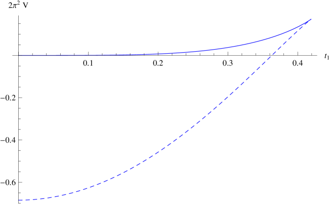
The two branches VM(t1)superscript𝑉𝑀subscript𝑡1V^{M}(t_{1}) and VV(t1)superscript𝑉𝑉subscript𝑡1V^{V}(t_{1}) of the effective potential are shown in figure 1.
Refer to caption

Figure 1: The two branches of the effective potential for t1subscript𝑡1t_{1} at level 1. The solid line is for 2π2VM(t1)2superscript𝜋2superscript𝑉𝑀subscript𝑡12\pi^{2}V^{M}(t_{1}) and the dashed line is for 2π2VV(t1)2superscript𝜋2superscript𝑉𝑉subscript𝑡12\pi^{2}V^{V}(t_{1}).

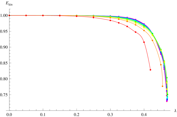
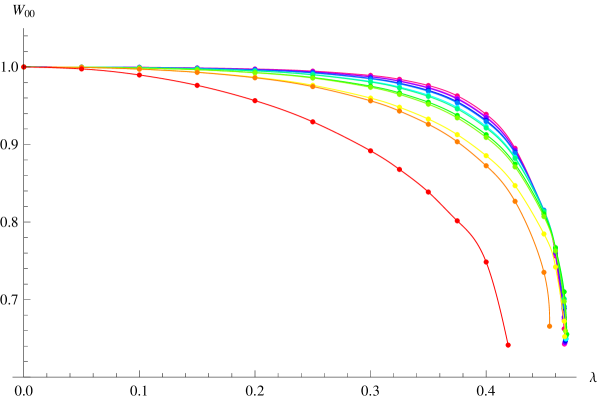
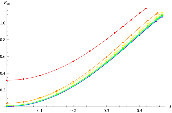
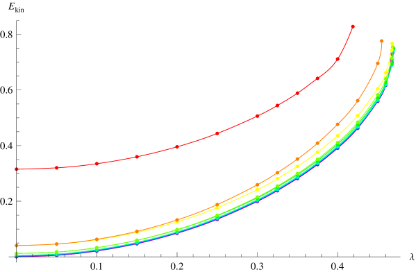
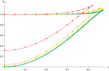
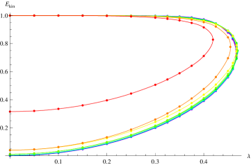
We expect an exactly flat potential for the marginal branch because the deformation by V1(t)subscript𝑉1𝑡V_{1}(t) is known to be exactly marginal. The potential VM(t1)superscript𝑉𝑀subscript𝑡1V^{M}(t_{1}) at level 1 is not exactly flat, but this is considered to be an artifact of level truncation. The higher-order analysis in level truncation shows that the effective potential for t1subscript𝑡1t_{1} on the marginal branch becomes flatter as the truncation level is increased, as expected. See figure 2.222The difference between the energy density Etotsubscript𝐸𝑡𝑜𝑡E_{tot} computed from the full action and the energy density Ekinsubscript𝐸𝑘𝑖𝑛E_{kin} computed from the kinetic term is proportional to t1subscript𝑡1t_{1} times the equation of motion for t1subscript𝑡1t_{1}. It has also been shown analytically that the coefficient in front of t14superscriptsubscript𝑡14t_{1}^{4} in VM(t1)superscript𝑉𝑀subscript𝑡1V^{M}(t_{1}) vanishes in the limit where the truncation level becomes infinite [28]. In this deformation, we can therefore use t1subscript𝑡1t_{1} as the label λSFTsubscript𝜆SFT\lambda_{\rm SFT} of approximate numerical solutions in level truncation.

On the other hand, the existence of the critical value of t1subscript𝑡1t_{1} does not seem to be an artifact of level truncation. The results at higher orders in figure 2 show that the critical value persists and the position of the critical value does not move significantly as the truncation level is increased. The analysis using level truncation thus indicates that the effective potential VM(t1)superscript𝑉𝑀subscript𝑡1V^{M}(t_{1}) on the marginal branch in Siegel gauge becomes exactly flat and terminates at a finite critical value in the limit where the truncation level becomes infinite.
Refer to caption
Refer to caption
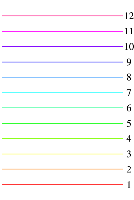
Figure 2: The energy density of the marginal and vacuum branches computed from the full action (the left graph) and from the kinetic term (the right graph). We have chosen t1subscript𝑡1t_{1} as the parameter λ𝜆\lambda of the branches. The energy density is measured from the tachyon vacuum and normalized by the D25-brane tension. In this and other figures, the colors follow the spectrum: higher level results are depicted using shorter wavelength colors. For explicit color coding, see figure 15.

3 Gauge-invariant observables and the closed string tadpole

In [27] Ellwood conjectured a relation between gauge-invariant observables of open string field theory discovered in [25, 26] and the closed string tadpole on a disk. The gauge-invariant observable W(ϕ,𝒱)𝑊italic-ϕ𝒱W(\phi\,,\mathcal{V}) for an open string state ϕitalic-ϕ\phi and an on-shell closed string vertex operator 𝒱𝒱\mathcal{V} is defined by the following correlation function on the upper half-plane:

W(ϕ,𝒱)=𝒱(i)fIϕ(0)UHP.𝑊italic-ϕ𝒱subscriptdelimited-⟨⟩𝒱𝑖subscript𝑓𝐼italic-ϕ0UHPW(\phi\,,\mathcal{V})=\langle\,\mathcal{V}(i)\,f_{I}\circ\phi(0)\,\rangle_{\rm UHP}\,. (3.1)

Here ϕ(0)italic-ϕ0\phi(0) is the operator corresponding to the state ϕitalic-ϕ\phi in the state-operator correspondence and we denoted by fIϕ(0)subscript𝑓𝐼italic-ϕ0f_{I}\circ\phi(0) the conformal transformation of ϕ(0)italic-ϕ0\phi(0) under the map fI(ξ)subscript𝑓𝐼𝜉f_{I}(\xi) associated with the identity state:

fI(ξ)=2ξ1ξ2.subscript𝑓𝐼𝜉2𝜉1superscript𝜉2f_{I}(\xi)=\frac{2\,\xi}{1-\xi^{2}}\,. (3.2)

The closed string tadpole on a unit disk defined in [27] is

𝒜disk(𝒱)=eiθ2πi𝒱(0)c(eiθ)disk.superscript𝒜disk𝒱superscript𝑒𝑖𝜃2𝜋𝑖subscriptdelimited-⟨⟩𝒱0𝑐superscript𝑒𝑖𝜃disk\mathcal{A}^{\rm disk}(\mathcal{V})=-\frac{e^{-i\theta}}{2\pi i}\,\langle\,\mathcal{V}(0)\,c(e^{i\theta})\,\rangle_{\rm disk}\,. (3.3)

This should be independent of θ𝜃\theta. The unit disk with a complex coordinate w𝑤w can be mapped to the upper half-plane of z𝑧z by the following conformal transformation:

z=i1w1+w.𝑧𝑖1𝑤1𝑤z=i\,\frac{1-w}{1+w}\,. (3.4)

The correlation function on a unit disk in (3.3) can be mapped under this conformal transformation to

𝒜disk(𝒱)=1π11+t2𝒱(i)c(t)UHPwitht=tanθ2.formulae-sequencesuperscript𝒜disk𝒱1𝜋11superscript𝑡2subscriptdelimited-⟨⟩𝒱𝑖𝑐𝑡UHPwith𝑡𝜃2\mathcal{A}^{\rm disk}(\mathcal{V})=-\frac{1}{\pi}\,\frac{1}{1+t^{2}}\,\langle\,\mathcal{V}(i)\,c(t)\,\rangle_{\rm UHP}\quad\text{with}\quad t=\tan\frac{\theta}{2}\,. (3.5)

It is easy to confirm that 𝒜disk(𝒱)superscript𝒜disk𝒱\mathcal{A}^{\rm disk}(\mathcal{V}) is independent of t𝑡t when the ghost part of 𝒱𝒱\mathcal{V} is cc~𝑐~𝑐c\tilde{c}. Ellwood conjectured the following relation:

W(Ψ,𝒱)=𝒜Ψdisk(𝒱)𝒜0disk(𝒱),𝑊Ψ𝒱subscriptsuperscript𝒜diskΨ𝒱subscriptsuperscript𝒜disk0𝒱W(\Psi,\mathcal{V})=\mathcal{A}^{\rm disk}_{\Psi}(\mathcal{V})-\mathcal{A}^{\rm disk}_{0}(\mathcal{V})\,, (3.6)

where 𝒜0disksubscriptsuperscript𝒜disk0\mathcal{A}^{\rm disk}_{0} is the closed string tadpole with the original boundary condition and 𝒜Ψdisksubscriptsuperscript𝒜diskΨ\mathcal{A}^{\rm disk}_{\Psi} is the closed string tadpole with the boundary condition corresponding to the classical solution ΨΨ\Psi. If the boundary CFT has marginal deformations labeled by λBCFTsubscript𝜆BCFT\lambda_{\rm BCFT}, we expect that the equation of motion of open string field theory has a one-parameter family of solutions labeled by λSFTsubscript𝜆SFT\lambda_{\rm SFT}. The left-hand side of (3.6) is a function of λSFTsubscript𝜆SFT\lambda_{\rm SFT}. The closed string tadpole appearing on the right-hand side of (3.6) is a function of λBCFTsubscript𝜆BCFT\lambda_{\rm BCFT}. We can thus obtain a map between λBCFTsubscript𝜆BCFT\lambda_{\rm BCFT} and λSFTsubscript𝜆SFT\lambda_{\rm SFT} from the conjectured relation (3.6).

We consider the marginal deformation by the cosine potential V1(t)subscript𝑉1𝑡V_{1}(t). We have to choose a closed string vertex operator 𝒱𝒱\mathcal{V} such that the one-point function 𝒜disk(𝒱)superscript𝒜disk𝒱\mathcal{A}^{\rm disk}(\mathcal{V}) has a nontrivial dependence on λBCFTsubscript𝜆BCFT\lambda_{\rm BCFT}. We choose

𝒱=2iαcc~X¯X.𝒱2𝑖superscript𝛼𝑐~𝑐𝑋¯𝑋\mathcal{V}=-\frac{2i}{\alpha^{\prime}}\,c\tilde{c}\partial X\bar{\partial}X\,. (3.7)

The normalization of 𝒱𝒱\mathcal{V} is the same as that in [29]. The dependence of 𝒜disk(𝒱)superscript𝒜disk𝒱\mathcal{A}^{\rm disk}(\mathcal{V}) on λBCFTsubscript𝜆BCFT\lambda_{\rm BCFT} can be easily determined using the boundary state [30], as studied, for example, in [31]. We have

𝒜disk(𝒱)cos( 2πλBCFT).proportional-tosuperscript𝒜disk𝒱2𝜋subscript𝜆BCFT\mathcal{A}^{\rm disk}(\mathcal{V})\propto\cos\,(\,2\pi\lambda_{\rm BCFT}\,)\,. (3.8)

It is a periodic function of λBCFTsubscript𝜆BCFT\lambda_{\rm BCFT}, and the Dirichlet boundary condition corresponds to the point λBCFT=1/2subscript𝜆BCFT12\lambda_{\rm BCFT}=1/2. The overall normalization of 𝒜disk(𝒱)superscript𝒜disk𝒱\mathcal{A}^{\rm disk}(\mathcal{V}) can be determined by evaluating the one-point function of 𝒱𝒱\mathcal{V} on a disk with the Neumann boundary condition, which corresponds to λBCFT=0subscript𝜆BCFT0\lambda_{\rm BCFT}=0. Our normalization of correlation functions on the upper half-plane is

c(z1)c(z2)c(z3)UHP=(z1z2)(z1z3)(z2z3).subscriptdelimited-⟨⟩𝑐subscript𝑧1𝑐subscript𝑧2𝑐subscript𝑧3UHPsubscript𝑧1subscript𝑧2subscript𝑧1subscript𝑧3subscript𝑧2subscript𝑧3\langle\,c(z_{1})\,c(z_{2})\,c(z_{3})\,\rangle_{\rm UHP}=(z_{1}-z_{2})(z_{1}-z_{3})(z_{2}-z_{3})\,. (3.9)

Here and in what follows we divide correlation functions by the spacetime volume factor. The one-point function of 𝒱𝒱\mathcal{V} on the upper half-plane with the Neumann boundary condition is given by

1π11+t2(2iα)cc~X¯X(i)c(t)UHP=12π.1𝜋11superscript𝑡22𝑖superscript𝛼subscriptdelimited-⟨⟩𝑐~𝑐𝑋¯𝑋𝑖𝑐𝑡UHP12𝜋-\frac{1}{\pi}\,\frac{1}{1+t^{2}}\,\Bigl{(}\,-\frac{2i}{\alpha^{\prime}}\,\Bigr{)}\langle\,c\tilde{c}\partial X\bar{\partial}X(i)\,c(t)\,\rangle_{\rm UHP}=-\frac{1}{2\pi}\,. (3.10)

This fixes the overall normalization of 𝒜disk(𝒱)superscript𝒜disk𝒱\mathcal{A}^{\rm disk}(\mathcal{V}) to give

𝒜disk(𝒱)=12πcos( 2πλBCFT).superscript𝒜disk𝒱12𝜋2𝜋subscript𝜆BCFT\mathcal{A}^{\rm disk}(\mathcal{V})=-\frac{1}{2\pi}\,\cos\,(\,2\pi\lambda_{\rm BCFT}\,)\,. (3.11)

Using the relation (3.6) we have

W(Ψ,𝒱)=12π[cos( 2πλBCFT)1].𝑊Ψ𝒱12𝜋delimited-[]2𝜋subscript𝜆BCFT1W(\Psi,\mathcal{V})=-\frac{1}{2\pi}\,\Bigl{[}\,\cos\,(\,2\pi\lambda_{\rm BCFT}\,)-1\,\Bigr{]}\,. (3.12)

It is convenient to introduce

WXX12πW(Ψ,𝒱)subscript𝑊𝑋𝑋12𝜋𝑊Ψ𝒱W_{XX}\equiv 1-2\pi\,W(\Psi,\mathcal{V}) (3.13)

for 𝒱𝒱\mathcal{V} given by (3.7). Then we have

WXX=cos( 2πλBCFT).subscript𝑊𝑋𝑋2𝜋subscript𝜆BCFTW_{XX}=\cos\,(\,2\pi\lambda_{\rm BCFT}\,)\,. (3.14)

As we mentioned before, the left-hand side is a function of λSFTsubscript𝜆SFT\lambda_{\rm SFT} labeling the solutions so that we can derive a map between λSFTsubscript𝜆SFT\lambda_{\rm SFT} and λBCFTsubscript𝜆BCFT\lambda_{\rm BCFT} from this relation. In particular, the value of the gauge-invariant observable for the solution corresponding to the Dirichlet boundary condition λBCFT=1/2subscript𝜆BCFT12\lambda_{\rm BCFT}=1/2 is given by WXX=1subscript𝑊𝑋𝑋1W_{XX}=-1.

4 Evaluation of the gauge-invariant observables

In this section we illustrate our computation of the gauge-invariant observables for the solutions corresponding to the cosine deformations reviewed in section 2. The solutions in Siegel gauge were constructed by Sen and Zwiebach in [22] up to level 4. We expand the string field in level \ell as follows:

|Ψ==0|Ψ().ketΨsuperscriptsubscript0ketsuperscriptΨ|\,\Psi\,\rangle=\sum_{\ell=0}^{\infty}|\,\Psi^{(\ell)}\,\rangle\,. (4.1)

The expressions up to level 4 in the notation used in section 3 of [22] are given by

|Ψ(0)=t0c1|0,|Ψ(1)=t1:cosX(0)α:c1|0,|Ψ(2)=(u0c1b1+v0L2X+w0L2)c1|0,|Ψ(3)=(u1c1b1+v1L2X+w1L2+z1L1XL1X)|φtwith|φt=:cosX(0)α:c1|0,|Ψ(4)=g~|p4+t2|χ+[aL4X+a¯L4+bL2XL2X+b¯L2L2+b^L2L2X+cc3b1+db3c1+eb2c2+(fL2X+f¯L2)c1b1]c1|0,\begin{split}|\,\Psi^{(0)}\,\rangle&=t_{0}\,c_{1}|0\rangle\,,\\ |\,\Psi^{(1)}\,\rangle&=t_{1}:\cos\frac{X(0)}{\sqrt{\alpha^{\prime}}}:c_{1}|0\rangle\,,\\ |\,\Psi^{(2)}\,\rangle&=\bigl{(}\,u_{0}\,c_{-1}\,b_{-1}+v_{0}\,L_{-2}^{X}+w_{0}\,L_{-2}^{\prime}\,\bigr{)}\,c_{1}\,|0\rangle\,,\\ |\,\Psi^{(3)}\,\rangle&=\bigl{(}\,u_{1}\,c_{-1}\,b_{-1}+v_{1}\,L_{-2}^{X}+w_{1}\,L_{-2}^{\prime}+z_{1}L_{-1}^{X}\,L_{-1}^{X}\,\bigr{)}\,|\varphi_{t}\rangle\quad\text{with}\quad|\varphi_{t}\rangle={}:\cos\frac{X(0)}{\sqrt{\alpha^{\prime}}}:c_{1}|0\rangle\,,\\ |\,\Psi^{(4)}\,\rangle&=\tilde{g}\,|p_{4}\rangle+t_{2}\,|\chi\rangle+\Bigl{[}\,a\,L_{-4}^{X}+\bar{a}\,L_{-4}^{\prime}+b\,L_{-2}^{X}\,L_{-2}^{X}+\bar{b}\,L_{-2}^{\prime}\,L_{-2}^{\prime}+\hat{b}\,L_{-2}^{\prime}\,L_{-2}^{X}\\ &\qquad\quad+c\,c_{-3}\,b_{-1}+d\,b_{-3}\,c_{-1}+e\,b_{-2}\,c_{-2}+(\,f\,L^{X}_{-2}+\bar{f}\,L^{\prime}_{-2}\,)\,c_{-1}\,b_{-1}\,\Bigr{]}\,c_{1}|0\rangle\,,\end{split} (4.2)

where LnXsuperscriptsubscript𝐿𝑛𝑋L_{n}^{X} are the Virasoro generators associated with the field X(t)𝑋𝑡X(t) describing the compactified direction and Lnsuperscriptsubscript𝐿𝑛L_{n}^{\prime} are the Virasoro generators associated with the rest of the matter fields. The primary field |p4ketsubscript𝑝4|p_{4}\rangle at level 4 is given by

|p4=(α3Xα1X34(α2X)212(α1X)4)c1|0,ketsubscript𝑝4superscriptsubscript𝛼3𝑋superscriptsubscript𝛼1𝑋34superscriptsuperscriptsubscript𝛼2𝑋212superscriptsuperscriptsubscript𝛼1𝑋4subscript𝑐1ket0|p_{4}\rangle=\bigl{(}\,\alpha_{-3}^{X}\,\alpha_{-1}^{X}-\frac{3}{4}\,(\alpha_{-2}^{X})^{2}-\frac{1}{2}\,(\alpha_{-1}^{X})^{4}\,\bigr{)}\,c_{1}\,|0\rangle\,, (4.3)

and |χket𝜒|\chi\rangle is

|χ=:cos2X(0)α:|0.|\chi\rangle={}:\cos\frac{2\,X(0)}{\sqrt{\alpha^{\prime}}}:|0\rangle\,. (4.4)

The gauge-invariant observable W(ϕ,𝒱)𝑊italic-ϕ𝒱W(\phi,\mathcal{V}) can be expressed as a BPZ inner product of ϕitalic-ϕ\phi with an open string state. For 𝒱𝒱\mathcal{V} given by (3.7), the gauge-invariant observable is

W(ϕ,𝒱)=ΦXX,ϕ,𝑊italic-ϕ𝒱subscriptΦ𝑋𝑋italic-ϕW(\phi,\mathcal{V})=\langle\,\Phi_{XX}\,,\phi\,\rangle\,, (4.5)

where the open string state ΦXXsubscriptΦ𝑋𝑋\Phi_{XX} has been constructed in [29] and is given by

|ΦXX=(144n,m=1imnmnαmXαnX)eEc0c1|0ketsubscriptΦ𝑋𝑋144superscriptsubscript𝑛𝑚1superscript𝑖𝑚𝑛𝑚𝑛subscriptsuperscript𝛼𝑋𝑚superscriptsubscript𝛼𝑛𝑋superscript𝑒𝐸subscript𝑐0subscript𝑐1ket0|\Phi_{XX}\rangle=\left(\frac{1}{4}-4\sum_{n,\,m=1}^{\infty}i^{m-n}\,m\,n\,\alpha^{X}_{-m}\,\alpha_{-n}^{X}\right)e^{E}c_{0}\,c_{1}\,|0\rangle (4.6)

with

E=12n=1(1)nnαnαn+n=1(1)ncnbn.𝐸12superscriptsubscript𝑛1superscript1𝑛𝑛subscript𝛼𝑛subscript𝛼𝑛superscriptsubscript𝑛1superscript1𝑛subscript𝑐𝑛subscript𝑏𝑛E=-\frac{1}{2}\sum_{n=1}^{\infty}\,\frac{(-1)^{n}}{n}\alpha_{-n}\cdot\alpha_{-n}+\sum_{n=1}^{\infty}\,(-1)^{n}\,c_{-n}\,b_{-n}\,. (4.7)

We denote the gauge-invariant observable W(Ψ,𝒱)𝑊Ψ𝒱W(\Psi,\mathcal{V}) truncated to level \ell by W()(Ψ,𝒱)superscript𝑊Ψ𝒱W^{(\ell)}(\Psi,\mathcal{V}). The quantity W(4)(Ψ,𝒱)superscript𝑊4Ψ𝒱W^{(4)}(\Psi,\mathcal{V}) is given by

W(4)(Ψ,𝒱)==04ΦXX,Ψ()=14t0+14u0318v0+258w0+314a254a¯+96316b+67516b¯77516b^+14e318f+258f¯+192g~.superscript𝑊4Ψ𝒱superscriptsubscript04subscriptΦ𝑋𝑋superscriptΨ14subscript𝑡014subscript𝑢0318subscript𝑣0258subscript𝑤0314𝑎254¯𝑎96316𝑏67516¯𝑏77516^𝑏14𝑒318𝑓258¯𝑓192~𝑔\begin{split}W^{(4)}(\Psi,\mathcal{V})&=\sum_{\ell=0}^{4}\,\langle\,\Phi_{XX},\Psi^{(\ell)}\,\rangle\\ &=\frac{1}{4}\,t_{0}+\frac{1}{4}\,u_{0}-\frac{31}{8}\,v_{0}+\frac{25}{8}\,w_{0}+\frac{31}{4}\,a-\frac{25}{4}\,\bar{a}+\frac{963}{16}\,b+\frac{675}{16}\,\bar{b}-\frac{775}{16}\,\hat{b}\\ &\quad~{}+\frac{1}{4}\,e-\frac{31}{8}\,f+\frac{25}{8}\,\bar{f}+192\,\tilde{g}\,.\end{split} (4.8)

Note that there are no contributions from Ψ(1)superscriptΨ1\Psi^{(1)} and Ψ(3)superscriptΨ3\Psi^{(3)} because of momentum conservation.

In the numerical solution constructed by Sen and Zwiebach in [22], the component fields t0subscript𝑡0t_{0}, t1subscript𝑡1t_{1}, u0subscript𝑢0u_{0}, \ldots are given as functions of t1subscript𝑡1t_{1}. We therefore obtain W(4)(Ψ,𝒱)superscript𝑊4Ψ𝒱W^{(4)}(\Psi,\mathcal{V}) for the solution as a function of t1subscript𝑡1t_{1}, which we are using as the label λSFTsubscript𝜆SFT\lambda_{\rm SFT}. This is how we compute the gauge-invariant observable as a function of λSFTsubscript𝜆SFT\lambda_{\rm SFT} in level truncation. We then compare the result with the expression (3.12) of the gauge-invariant observable as a function of λBCFTsubscript𝜆BCFT\lambda_{\rm BCFT} to find a relation between λSFTsubscript𝜆SFT\lambda_{\rm SFT} and λBCFTsubscript𝜆BCFT\lambda_{\rm BCFT} numerically.

5 Numerical evaluation to level 12

The method illustrated in the preceding section at level 4 can be extended to higher levels. We had generated all required vertices using the conservation laws of [32] and then solved the equations of motion by Newton’s iterative method.333 Newton’s method requires a choice of an initial approximate solution, which is then iteratively improved to any desired accuracy. We define it as Ψ(i)ψ(i1)ψ(i)normsuperscriptΨ𝑖superscript𝜓𝑖1normsuperscript𝜓𝑖\frac{\|\Psi^{(i)}-\psi^{(i-1)}\|}{\|\psi^{(i)}\|} and stop the iteration when we reach 108superscript10810^{-8}. The norm is defined, as usual, by a square root of the sum of coefficients squared in the basis formed by α𝛼\alpha oscillators of the compact direction, bc𝑏𝑐bc oscillators of the ghost sector, and the Virasoro generators in the rest of the matter sector. As the starting point we either used results for the solution with the same λ𝜆\lambda found at lower level or, sometimes more efficiently, used a different solution with a neighboring value of λ𝜆\lambda at the same level. With the help of a computer cluster we were able to perform all our computations to level (12,36)1236(12,36).

To avoid possible confusion between the marginal and vacuum branches, but also out of curiosity, we studied numerically both branches for various values of λ𝜆\lambda, up to the critical level-dependent λcritsubscript𝜆𝑐𝑟𝑖𝑡\lambda_{crit}, where both branches meet. The value of λcritsubscript𝜆𝑐𝑟𝑖𝑡\lambda_{crit} at level 1 is given by the simple analytic formula (2.5). At higher levels we employed the interval bisection method and studied whether Newton’s method converges for given λ𝜆\lambda. The results are given in table 1.

LλcritLλcrit10.41902670.46923920.45486680.46864530.46790090.46862340.468614100.46816050.469761110.46810960.469100120.467748missing-subexpressionmissing-subexpressionmissing-subexpressionmissing-subexpression𝐿subscript𝜆𝑐𝑟𝑖𝑡𝐿subscript𝜆𝑐𝑟𝑖𝑡missing-subexpressionmissing-subexpressionmissing-subexpressionmissing-subexpression10.41902670.46923920.45486680.46864530.46790090.46862340.468614100.46816050.469761110.46810960.469100120.467748\begin{array}[]{|c|c|r|c|}\hline\cr L&\lambda_{crit}&L&\lambda_{crit}\\ \hline\cr 1&0.419026&7&0.469239\\ 2&0.454866&8&0.468645\\ 3&0.467900&9&0.468623\\ 4&0.468614&10&0.468160\\ 5&0.469761&11&0.468109\\ 6&0.469100&12&0.467748\\ \hline\cr\end{array}
Table 1: Results for λcritsubscript𝜆𝑐𝑟𝑖𝑡\lambda_{crit} at levels L=1,,12𝐿112L=1,\ldots,12. The values are rounded down to six digits, so that the solution still exists for these values. It can be found within about 5 iterations if we use as the starting point for Newton’s method the highest λ𝜆\lambda solution found in the previous steps at the same level. Increasing the last digit by one, Newton’s method would not anymore converge within 50 iterations at lower levels and at least 10 iterations at level 12.

Interestingly, the critical value grows at low levels and is largest at level 5, and after one oscillation it monotonically decreases. Simple linear extrapolation in 1/L1𝐿1/L to the infinite level gives the critical value of about 0.4660.4660.466. Values of the energy and the gauge-invariant observables at λcritsubscript𝜆𝑐𝑟𝑖𝑡\lambda_{crit} for each given level L=1,,12𝐿112L=1,\ldots,12 are presented in table 3 of appendix A.

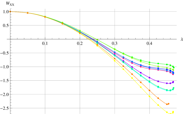
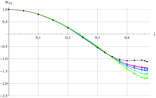
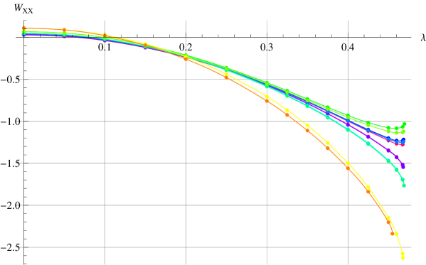
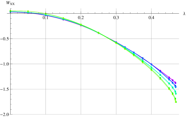
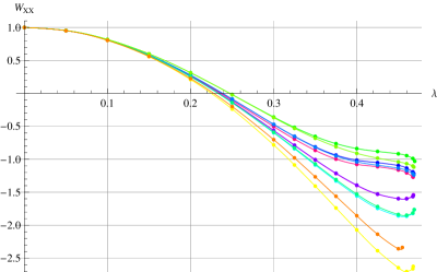
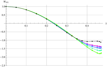
We have constructed the marginal and vacuum branches for about 15 different values of λ𝜆\lambda. Figure 2, presented in section 2, shows the energy density of the marginal and vacuum branches meeting at λcritsubscript𝜆𝑐𝑟𝑖𝑡\lambda_{crit}. The quantity WXXsubscript𝑊𝑋𝑋W_{XX} defined in (3.13) on the marginal branch for various levels is plotted in the left graph of figure 3. Its dependence on the level is rather erratic, so we tried to apply Padé-Borel resummation of contributions of different levels for each solution. The right graph of figure 3 shows the resulting improved values of WXXsubscript𝑊𝑋𝑋W_{XX}, together with a simple extrapolation to the infinite level. More data are presented in appendix A.
Refer to caption
Refer to caption
Figure 3: The values of WXXsubscript𝑊𝑋𝑋W_{XX} at levels L=2,,12𝐿212L=2,\ldots,12 (left) and their Padé-Borel improvements at levels L=4,,12𝐿412L=4,\ldots,12, together with a fit to the infinite level in black (right).

One may notice that starting at level 3 the results at odd levels are close to the values found at the previous even level. The reason is most likely that at even levels new fields with zero momentum appear, and they seem to have larger influence than the fields with nonzero momentum. The similarity of odd and even levels is even greater for WXXsubscript𝑊𝑋𝑋W_{XX} because it receives contributions only from fields at even levels, meaning that any change at odd levels can arise only from the change of the solution and not from adding new fields.

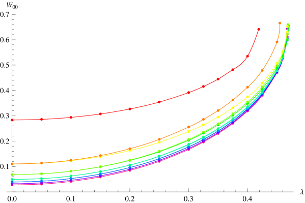
Table 2 summarizes linear extrapolations in 1/L1𝐿1/L of various quantities of interest to the infinite level together with the estimated statistical error. We estimate the error by considering extrapolations using different numbers of data points and computing the sample standard deviation for such results. For WXXsubscript𝑊𝑋𝑋W_{XX} we use the Padé-Borel resummed version. We also computed W00subscript𝑊00W_{00} defined by

W00=1+2πW(Ψ,𝒱)subscript𝑊0012𝜋𝑊Ψ𝒱W_{00}=1+2\pi\,W(\Psi,\mathcal{V}) (5.1)

with

𝒱=2iαcc~X0¯X0.𝒱2𝑖superscript𝛼𝑐~𝑐superscript𝑋0¯superscript𝑋0\mathcal{V}=-\frac{2i}{\alpha^{\prime}}\,c\tilde{c}\partial X^{0}\bar{\partial}X^{0}\,. (5.2)

Up to approximately λ=0.325𝜆0.325\lambda=0.325 the extrapolated values of the energy density Etotsubscript𝐸𝑡𝑜𝑡E_{tot} computed from the full action, the energy density Ekinsubscript𝐸𝑘𝑖𝑛E_{kin} computed from the kinetic term, and W00subscript𝑊00W_{00} are consistent with the expected value 1. Apparently, for higher values of λ𝜆\lambda our method underestimates the error of the extrapolated values.
λEtotσEtotEkinσEkinW00σW00WXXσWXX0.051.6.3×1071.2.1×1071.0.000070.94930.00180.11.0.000011.3.4×1061.0.000280.80510.00250.151.0.0000511.0.0000181.00010.000660.56860.00460.21.0.000161.0.0000571.0.00120.25720.0140.250.99990.00041.0.000140.99960.0020.13380.0120.30.99990.000830.99970.000260.99780.00290.54990.00220.3251.0.00110.9990.000330.99540.00340.74490.010.351.00040.00150.99720.000410.99050.00390.90960.0130.3751.00160.00190.9920.000520.97980.00431.02510.0270.41.00490.00230.97810.000350.95650.00461.0760.0440.4251.0130.00280.94330.00130.90750.0051.06490.0590.451.03210.00350.86680.00460.81160.00641.05620.0760.461.04510.00370.81120.00670.74530.00771.07780.0850.46751.05850.00390.71240.0190.63260.021.11490.092missing-subexpressionmissing-subexpressionmissing-subexpressionmissing-subexpressionmissing-subexpressionmissing-subexpressionmissing-subexpressionmissing-subexpressionmissing-subexpression𝜆subscript𝐸𝑡𝑜𝑡subscript𝜎subscript𝐸𝑡𝑜𝑡subscript𝐸𝑘𝑖𝑛subscript𝜎subscript𝐸𝑘𝑖𝑛subscript𝑊00subscript𝜎𝑊00subscript𝑊𝑋𝑋subscript𝜎subscript𝑊𝑋𝑋missing-subexpressionmissing-subexpressionmissing-subexpressionmissing-subexpressionmissing-subexpressionmissing-subexpressionmissing-subexpressionmissing-subexpressionmissing-subexpression0.0516.3superscript10712.1superscript10710.000070.94930.00180.110.0000113.4superscript10610.000280.80510.00250.1510.00005110.0000181.00010.000660.56860.00460.210.0001610.00005710.00120.25720.0140.250.99990.000410.000140.99960.0020.13380.0120.30.99990.000830.99970.000260.99780.00290.54990.00220.32510.00110.9990.000330.99540.00340.74490.010.351.00040.00150.99720.000410.99050.00390.90960.0130.3751.00160.00190.9920.000520.97980.00431.02510.0270.41.00490.00230.97810.000350.95650.00461.0760.0440.4251.0130.00280.94330.00130.90750.0051.06490.0590.451.03210.00350.86680.00460.81160.00641.05620.0760.461.04510.00370.81120.00670.74530.00771.07780.0850.46751.05850.00390.71240.0190.63260.021.11490.092\begin{array}[]{|l|ll|ll|ll|ll|}\hline\cr\lambda&E_{tot}&\sigma_{E_{tot}}&E_{kin}&\sigma_{E_{kin}}&W_{00}&\sigma_{W00}&W_{XX}&\sigma_{W_{XX}}\\ \hline\cr 0.05&1.&6.3\times 10^{-7}&1.&2.1\times 10^{-7}&1.&0.00007&0.9493&0.0018\\ 0.1&1.&0.00001&1.&3.4\times 10^{-6}&1.&0.00028&0.8051&0.0025\\ 0.15&1.&0.000051&1.&0.000018&1.0001&0.00066&0.5686&0.0046\\ 0.2&1.&0.00016&1.&0.000057&1.&0.0012&0.2572&0.014\\ 0.25&0.9999&0.0004&1.&0.00014&0.9996&0.002&-0.1338&0.012\\ 0.3&0.9999&0.00083&0.9997&0.00026&0.9978&0.0029&-0.5499&0.0022\\ 0.325&1.&0.0011&0.999&0.00033&0.9954&0.0034&-0.7449&0.01\\ 0.35&1.0004&0.0015&0.9972&0.00041&0.9905&0.0039&-0.9096&0.013\\ 0.375&1.0016&0.0019&0.992&0.00052&0.9798&0.0043&-1.0251&0.027\\ 0.4&1.0049&0.0023&0.9781&0.00035&0.9565&0.0046&-1.076&0.044\\ 0.425&1.013&0.0028&0.9433&0.0013&0.9075&0.005&-1.0649&0.059\\ 0.45&1.0321&0.0035&0.8668&0.0046&0.8116&0.0064&-1.0562&0.076\\ 0.46&1.0451&0.0037&0.8112&0.0067&0.7453&0.0077&-1.0778&0.085\\ 0.4675&1.0585&0.0039&0.7124&0.019&0.6326&0.02&-1.1149&0.092\\ \hline\cr\end{array}
Table 2: Extrapolation to the infinite level and its possible statistical error for the four basic quantities computed at several values of λ𝜆\lambda on the marginal branch. Up to about λ=0.325𝜆0.325\lambda=0.325 the first three observables are within the 3σ3𝜎3\sigma tolerance away from the expected value of 111.
Refer to caption
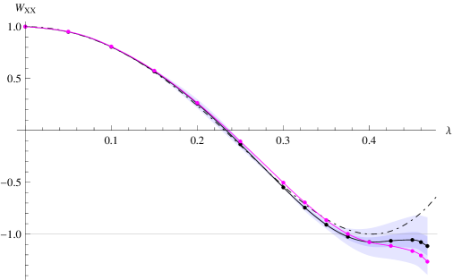
Figure 4: Extrapolation to the infinite level of the Padé-Borel resummed version of WXXsubscript𝑊𝑋𝑋W_{XX}. The black solid line is the infinite-level fit itself, while the shaded regions around it indicate σ𝜎\sigma and 3σ3𝜎3\sigma uncertainty ranges in the extrapolation. The magenta line shows the (unimproved) data at level 12 for comparison. The black dot-dashed line is the one-parameter fit of the form cos(2π(λ+aλ3))2𝜋𝜆𝑎superscript𝜆3\cos\left(2\pi(\lambda+a\lambda^{3})\right).

The results for WXXsubscript𝑊𝑋𝑋W_{XX} together with its estimated error are presented in figure 4. The one-parameter fit of the form cos(2π(λ+aλ3))2𝜋𝜆𝑎superscript𝜆3\cos\left(2\pi(\lambda+a\lambda^{3})\right) is also shown, where the constant a𝑎a has been fitted so that the extrapolation to the infinite level coincides with the boundary CFT result at lower values of λ𝜆\lambda. The best fit value for a𝑎a is about 0.990.990.99 at level 4 and grows at higher levels. For the extrapolation to the infinite level we find a1.48𝑎1.48a\approx 1.48. It would be interesting to calculate this value analytically. The results of WXXsubscript𝑊𝑋𝑋W_{XX} qualitatively agree with the analysis by Sen [23] using the energy-momentum tensor and are consistent with the picture that the finite range of the branch covers one fundamental domain of the periodic moduli space. While our results do not provide sufficient evidence that the branch covers exactly one fundamental domain, we can safely exclude the possibility that the branch covers the fundamental domain many times. We can also exclude the opposite possibility that the branch covers, say, less than 75% of the fundamental domain. If the branch indeed covers exactly one fundamental domain, it would be interesting to understand why it is the case.

6 Discussion

In this paper we presented a method of constructing a map between the deformation parameter λBCFTsubscript𝜆BCFT\lambda_{\rm BCFT} of boundary CFT and the parameter λSFTsubscript𝜆SFT\lambda_{\rm SFT} labeling solutions of open string field theory for marginal deformations. While we applied our method to the specific problem of covering moduli for solutions in Siegel gauge, the basic idea is universal and we can use it for other problems. For example, a similar problem for the system of separated D-branes has recently been discussed in [33, 34] and it would be interesting to compute the gauge-invariant observables in the system.

If we construct the boundary state from numerical solutions following the proposal in [35], we will be able to obtain more information on the boundary CFT. However, construction of the boundary state for numerical solutions seems to be challenging. In particular, the closed string state proposed in [35] is conjectured to reproduce the boundary state up to a BRST-exact term, and such a BRST-exact term would obscure the boundary state especially for approximate solutions constructed numerically.444 After this paper was submitted to arXiv, another approach to the construction of the boundary state was proposed in [36], which is more suitable for the application to numerical solutions.

Our results are qualitatively consistent with the analysis by Sen [23] using the energy-momentum tensor. This is not unexpected because both methods are based on coupling to an infinitesimal closed string field. However, the closed string is described by an unintegrated vertex operator in the gauge-invariant observables and also in the boundary state construction in [35], while the infinitesimal change in the closed string background is related more closely to an integrated vertex operator. It would be an interesting problem to convert the unintegrated vertex operator to the integrated vertex operator in the framework of the gauge-invariant observables and the boundary state construction [35].


Acknowledgments

We would like to thank Ted Erler, Mitsuhiro Kato, Michael Kiermaier, Carlo Maccaferri and Barton Zwiebach for helpful discussions and to Masaki Murata for careful reading of the manuscript. The access to computing and storage facilities owned by parties and projects contributing to the Czech National Grid Infrastructure MetaCentrum, provided under the programme “Projects of Large Infrastructure for Research, Development, and Innovations” (LM2010005), and to CERIT-SC computing facilities provided under the programme Center CERIT Scientific Cloud, part of the Operational Program Research and Development for Innovations, reg. no. CZ. 1.05/3.2.00/08.0144 is highly appreciated. The work of Y.O. was supported in part by Grant-in-Aid for Scientific Research (B) No. 20340048 and Grant-in-Aid for Scientific Research (C) No. 24540254 from the Japan Society for the Promotion of Science (JSPS). The work of M.S. was supported by the EURYI grant GACR EYI/07/E010 from EUROHORC and ESF. The work of Y.O. and M.S. was also supported in part by the MŠMT contract No. LH11106 and by JSPS and the Academy of Sciences of the Czech Republic (ASCR) under the Research Cooperative Program between Japan and the Czech Republic.

Appendix A Tables of numerical results

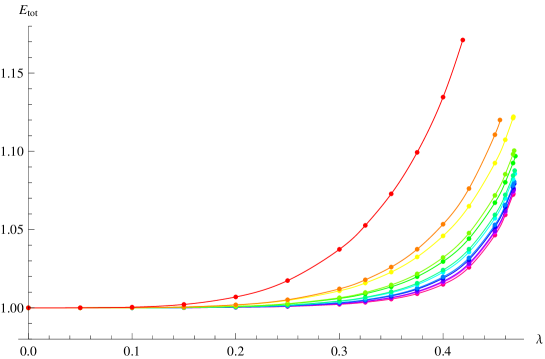
In the following figures Etotsubscript𝐸𝑡𝑜𝑡E_{tot} denotes the energy density computed from the full action and Ekinsubscript𝐸𝑘𝑖𝑛E_{kin} denotes the energy density computed from the kinetic term.
L/λ00.050.10.150.20.250.30.325111.000031.000421.002161.006941.017391.037371.05266211.000011.00011.000561.00191.005151.012091.01789311.000011.00011.000541.001791.004731.010841.01585411.1.000051.000271.000951.002641.006441.00976511.1.000051.000271.000911.002491.005981.009611.1.000031.000181.000621.001751.004361.00672711.1.000031.000171.000611.001681.004131.00634811.1.000021.000131.000461.001311.00331.00515911.1.000021.000131.000451.001271.003171.004921011.1.000021.00011.000371.001041.002661.004181111.1.000021.00011.000361.001021.002581.004031211.1.000021.000091.000311.000871.002231.00353missing-subexpressionmissing-subexpressionmissing-subexpressionmissing-subexpressionmissing-subexpressionmissing-subexpressionmissing-subexpressionmissing-subexpressionmissing-subexpression𝐿𝜆00.050.10.150.20.250.30.325missing-subexpressionmissing-subexpressionmissing-subexpressionmissing-subexpressionmissing-subexpressionmissing-subexpressionmissing-subexpressionmissing-subexpressionmissing-subexpression111.000031.000421.002161.006941.017391.037371.05266211.000011.00011.000561.00191.005151.012091.01789311.000011.00011.000541.001791.004731.010841.015854111.000051.000271.000951.002641.006441.009765111.000051.000271.000911.002491.005981.0096111.000031.000181.000621.001751.004361.006727111.000031.000171.000611.001681.004131.006348111.000021.000131.000461.001311.00331.005159111.000021.000131.000451.001271.003171.0049210111.000021.00011.000371.001041.002661.0041811111.000021.00011.000361.001021.002581.0040312111.000021.000091.000311.000871.002231.00353\begin{array}[]{|l|llllllll|}\hline\cr L/\lambda&0&0.05&0.1&0.15&0.2&0.25&0.3&0.325\\ \hline\cr 1&1&1.00003&1.00042&1.00216&1.00694&1.01739&1.03737&1.05266\\ 2&1&1.00001&1.0001&1.00056&1.0019&1.00515&1.01209&1.01789\\ 3&1&1.00001&1.0001&1.00054&1.00179&1.00473&1.01084&1.01585\\ 4&1&1.&1.00005&1.00027&1.00095&1.00264&1.00644&1.00976\\ 5&1&1.&1.00005&1.00027&1.00091&1.00249&1.00598&1.009\\ 6&1&1.&1.00003&1.00018&1.00062&1.00175&1.00436&1.00672\\ 7&1&1.&1.00003&1.00017&1.00061&1.00168&1.00413&1.00634\\ 8&1&1.&1.00002&1.00013&1.00046&1.00131&1.0033&1.00515\\ 9&1&1.&1.00002&1.00013&1.00045&1.00127&1.00317&1.00492\\ 10&1&1.&1.00002&1.0001&1.00037&1.00104&1.00266&1.00418\\ 11&1&1.&1.00002&1.0001&1.00036&1.00102&1.00258&1.00403\\ 12&1&1.&1.00002&1.00009&1.00031&1.00087&1.00223&1.00353\\ \hline\cr\end{array}
L/λ0.350.3750.40.4250.450.460.467511.072821.099341.1346321.026041.037441.053421.076211.1106131.022821.032491.045951.064921.092481.107381.1212241.014611.021711.032151.047751.071831.085371.0981651.013421.019921.029571.044211.067191.080231.0924961.010291.015721.024131.037471.059381.072191.0844971.009671.014781.022771.035651.057211.069951.0822181.0081.012491.019771.031921.053021.065751.0781891.007631.011911.018911.03081.051771.064531.07701101.006581.010451.016961.028371.049121.061931.0746111.006321.010051.016361.027591.048311.061171.07391121.00561.009021.014971.025871.046471.05941.07233missing-subexpressionmissing-subexpressionmissing-subexpressionmissing-subexpressionmissing-subexpressionmissing-subexpressionmissing-subexpressionmissing-subexpression𝐿𝜆0.350.3750.40.4250.450.460.4675missing-subexpressionmissing-subexpressionmissing-subexpressionmissing-subexpressionmissing-subexpressionmissing-subexpressionmissing-subexpressionmissing-subexpression11.072821.099341.1346321.026041.037441.053421.076211.1106131.022821.032491.045951.064921.092481.107381.1212241.014611.021711.032151.047751.071831.085371.0981651.013421.019921.029571.044211.067191.080231.0924961.010291.015721.024131.037471.059381.072191.0844971.009671.014781.022771.035651.057211.069951.0822181.0081.012491.019771.031921.053021.065751.0781891.007631.011911.018911.03081.051771.064531.07701101.006581.010451.016961.028371.049121.061931.0746111.006321.010051.016361.027591.048311.061171.07391121.00561.009021.014971.025871.046471.05941.07233\begin{array}[]{|l|lllllll|}\hline\cr L/\lambda&0.35&0.375&0.4&0.425&0.45&0.46&0.4675\\ \hline\cr 1&1.07282&1.09934&1.13463&-&-&-&-\\ 2&1.02604&1.03744&1.05342&1.07621&1.11061&-&-\\ 3&1.02282&1.03249&1.04595&1.06492&1.09248&1.10738&1.12122\\ 4&1.01461&1.02171&1.03215&1.04775&1.07183&1.08537&1.09816\\ 5&1.01342&1.01992&1.02957&1.04421&1.06719&1.08023&1.09249\\ 6&1.01029&1.01572&1.02413&1.03747&1.05938&1.07219&1.08449\\ 7&1.00967&1.01478&1.02277&1.03565&1.05721&1.06995&1.08221\\ 8&1.008&1.01249&1.01977&1.03192&1.05302&1.06575&1.07818\\ 9&1.00763&1.01191&1.01891&1.0308&1.05177&1.06453&1.07701\\ 10&1.00658&1.01045&1.01696&1.02837&1.04912&1.06193&1.0746\\ 11&1.00632&1.01005&1.01636&1.02759&1.04831&1.06117&1.07391\\ 12&1.0056&1.00902&1.01497&1.02587&1.04647&1.0594&1.07233\\ \hline\cr\end{array}
Refer to caption
Figure 5: Etotsubscript𝐸𝑡𝑜𝑡E_{tot} for the marginal branch at levels L=1,,12𝐿112L=1,\ldots,12. For the color legend, see figure 15.
L/λ00.050.10.150.20.250.30.325110.9999910.9998570.9992480.9974830.9933250.9844060.976723210.9999980.9999620.9997760.9991340.9973110.9926530.988209310.9999980.9999640.9997960.9992430.9977330.9939410.990326410.9999990.9999810.9998870.9995410.9984870.9955190.99246510.9999990.9999820.9998930.9995810.9986450.9960080.993251610.9999990.9999880.9999250.9996920.9989490.9967130.994255710.9999990.9999880.9999280.9997110.9990280.9969740.994692811.0.9999910.9999440.9997690.9991940.9973870.99531911.0.9999910.9999460.9997790.9992410.997550.995591011.0.9999930.9999560.9998150.9993460.9978250.9960171111.0.9999930.9999570.9998210.9993760.9979360.9962151211.0.9999940.9999630.9998450.9994490.9981340.99653missing-subexpressionmissing-subexpressionmissing-subexpressionmissing-subexpressionmissing-subexpressionmissing-subexpressionmissing-subexpressionmissing-subexpressionmissing-subexpression𝐿𝜆00.050.10.150.20.250.30.325missing-subexpressionmissing-subexpressionmissing-subexpressionmissing-subexpressionmissing-subexpressionmissing-subexpressionmissing-subexpressionmissing-subexpressionmissing-subexpression110.9999910.9998570.9992480.9974830.9933250.9844060.976723210.9999980.9999620.9997760.9991340.9973110.9926530.988209310.9999980.9999640.9997960.9992430.9977330.9939410.990326410.9999990.9999810.9998870.9995410.9984870.9955190.99246510.9999990.9999820.9998930.9995810.9986450.9960080.993251610.9999990.9999880.9999250.9996920.9989490.9967130.994255710.9999990.9999880.9999280.9997110.9990280.9969740.9946928110.9999910.9999440.9997690.9991940.9973870.995319110.9999910.9999460.9997790.9992410.997550.9955910110.9999930.9999560.9998150.9993460.9978250.99601711110.9999930.9999570.9998210.9993760.9979360.99621512110.9999940.9999630.9998450.9994490.9981340.99653\begin{array}[]{|l|llllllll|}\hline\cr L/\lambda&0&0.05&0.1&0.15&0.2&0.25&0.3&0.325\\ \hline\cr 1&1&0.999991&0.999857&0.999248&0.997483&0.993325&0.984406&0.976723\\ 2&1&0.999998&0.999962&0.999776&0.999134&0.997311&0.992653&0.988209\\ 3&1&0.999998&0.999964&0.999796&0.999243&0.997733&0.993941&0.990326\\ 4&1&0.999999&0.999981&0.999887&0.999541&0.998487&0.995519&0.99246\\ 5&1&0.999999&0.999982&0.999893&0.999581&0.998645&0.996008&0.993251\\ 6&1&0.999999&0.999988&0.999925&0.999692&0.998949&0.996713&0.994255\\ 7&1&0.999999&0.999988&0.999928&0.999711&0.999028&0.996974&0.994692\\ 8&1&1.&0.999991&0.999944&0.999769&0.999194&0.997387&0.99531\\ 9&1&1.&0.999991&0.999946&0.999779&0.999241&0.99755&0.99559\\ 10&1&1.&0.999993&0.999956&0.999815&0.999346&0.997825&0.996017\\ 11&1&1.&0.999993&0.999957&0.999821&0.999376&0.997936&0.996215\\ 12&1&1.&0.999994&0.999963&0.999845&0.999449&0.998134&0.99653\\ \hline\cr\end{array}
L/λ0.350.3750.40.4250.450.460.467510.9653170.9475080.91563320.9812810.9703610.9525950.9212380.84466830.9846770.9757660.9614010.9371090.8902340.8537960.78754840.9874060.9789930.9647450.9396570.8902150.8522610.79204950.9886080.9806840.9668870.9419890.8925730.8555880.8036160.9899510.9822940.9683870.9423430.8894220.8493830.79042170.9906290.9832380.9694480.9429810.8886950.8479730.78934580.99150.984330.9704520.9429550.8856790.84250.77696190.9919520.9849710.9711280.9430990.8844120.840510.774259100.9925810.9857940.9718880.9429360.8817790.8359930.762596110.992910.9862750.9723770.9428870.880490.8341320.759646120.9933910.986930.9729850.9426610.8782280.8304230.747139missing-subexpressionmissing-subexpressionmissing-subexpressionmissing-subexpressionmissing-subexpressionmissing-subexpressionmissing-subexpressionmissing-subexpression𝐿𝜆0.350.3750.40.4250.450.460.4675missing-subexpressionmissing-subexpressionmissing-subexpressionmissing-subexpressionmissing-subexpressionmissing-subexpressionmissing-subexpressionmissing-subexpression10.9653170.9475080.91563320.9812810.9703610.9525950.9212380.84466830.9846770.9757660.9614010.9371090.8902340.8537960.78754840.9874060.9789930.9647450.9396570.8902150.8522610.79204950.9886080.9806840.9668870.9419890.8925730.8555880.8036160.9899510.9822940.9683870.9423430.8894220.8493830.79042170.9906290.9832380.9694480.9429810.8886950.8479730.78934580.99150.984330.9704520.9429550.8856790.84250.77696190.9919520.9849710.9711280.9430990.8844120.840510.774259100.9925810.9857940.9718880.9429360.8817790.8359930.762596110.992910.9862750.9723770.9428870.880490.8341320.759646120.9933910.986930.9729850.9426610.8782280.8304230.747139\begin{array}[]{|l|lllllll|}\hline\cr L/\lambda&0.35&0.375&0.4&0.425&0.45&0.46&0.4675\\ \hline\cr 1&0.965317&0.947508&0.915633&-&-&-&-\\ 2&0.981281&0.970361&0.952595&0.921238&0.844668&-&-\\ 3&0.984677&0.975766&0.961401&0.937109&0.890234&0.853796&0.787548\\ 4&0.987406&0.978993&0.964745&0.939657&0.890215&0.852261&0.792049\\ 5&0.988608&0.980684&0.966887&0.941989&0.892573&0.855588&0.80361\\ 6&0.989951&0.982294&0.968387&0.942343&0.889422&0.849383&0.790421\\ 7&0.990629&0.983238&0.969448&0.942981&0.888695&0.847973&0.789345\\ 8&0.9915&0.98433&0.970452&0.942955&0.885679&0.8425&0.776961\\ 9&0.991952&0.984971&0.971128&0.943099&0.884412&0.84051&0.774259\\ 10&0.992581&0.985794&0.971888&0.942936&0.881779&0.835993&0.762596\\ 11&0.99291&0.986275&0.972377&0.942887&0.88049&0.834132&0.759646\\ 12&0.993391&0.98693&0.972985&0.942661&0.878228&0.830423&0.747139\\ \hline\cr\end{array}
Refer to caption
Figure 6: Ekinsubscript𝐸𝑘𝑖𝑛E_{kin} for the marginal branch at levels L=1,,12𝐿112L=1,\ldots,12.
L/λ00.050.10.150.20.250.30.325110.997440.9896480.9762570.9565560.9292480.8918550.867871210.9993270.997160.9930280.9860420.9746810.9563290.94316310.9993290.9972020.9932460.9867320.9763690.959850.94805410.999660.9985490.9963630.992480.985720.9737960.964585510.9996610.9985650.9964450.9927470.9863960.9752260.966539610.9997730.9990250.9975240.9947840.9898160.9805260.972937710.9997740.9990330.9975670.9949260.9901910.9813620.974112810.9998350.9992860.9981730.99610.9922360.9847010.978279910.9998350.9992910.9981970.9961860.992470.9852480.979071010.9998670.9994230.9985180.9968160.9935960.9871510.9814981110.9998670.9994260.9985340.9968740.9937560.9875390.9820731210.9998910.9995280.9987810.9973620.9946360.9890570.98404missing-subexpressionmissing-subexpressionmissing-subexpressionmissing-subexpressionmissing-subexpressionmissing-subexpressionmissing-subexpressionmissing-subexpressionmissing-subexpression𝐿𝜆00.050.10.150.20.250.30.325missing-subexpressionmissing-subexpressionmissing-subexpressionmissing-subexpressionmissing-subexpressionmissing-subexpressionmissing-subexpressionmissing-subexpressionmissing-subexpression110.997440.9896480.9762570.9565560.9292480.8918550.867871210.9993270.997160.9930280.9860420.9746810.9563290.94316310.9993290.9972020.9932460.9867320.9763690.959850.94805410.999660.9985490.9963630.992480.985720.9737960.964585510.9996610.9985650.9964450.9927470.9863960.9752260.966539610.9997730.9990250.9975240.9947840.9898160.9805260.972937710.9997740.9990330.9975670.9949260.9901910.9813620.974112810.9998350.9992860.9981730.99610.9922360.9847010.978279910.9998350.9992910.9981970.9961860.992470.9852480.979071010.9998670.9994230.9985180.9968160.9935960.9871510.9814981110.9998670.9994260.9985340.9968740.9937560.9875390.9820731210.9998910.9995280.9987810.9973620.9946360.9890570.98404\begin{array}[]{|l|llllllll|}\hline\cr L/\lambda&0&0.05&0.1&0.15&0.2&0.25&0.3&0.325\\ \hline\cr 1&1&0.99744&0.989648&0.976257&0.956556&0.929248&0.891855&0.867871\\ 2&1&0.999327&0.99716&0.993028&0.986042&0.974681&0.956329&0.94316\\ 3&1&0.999329&0.997202&0.993246&0.986732&0.976369&0.95985&0.94805\\ 4&1&0.99966&0.998549&0.996363&0.99248&0.98572&0.973796&0.964585\\ 5&1&0.999661&0.998565&0.996445&0.992747&0.986396&0.975226&0.966539\\ 6&1&0.999773&0.999025&0.997524&0.994784&0.989816&0.980526&0.972937\\ 7&1&0.999774&0.999033&0.997567&0.994926&0.990191&0.981362&0.974112\\ 8&1&0.999835&0.999286&0.998173&0.9961&0.992236&0.984701&0.978279\\ 9&1&0.999835&0.999291&0.998197&0.996186&0.99247&0.985248&0.97907\\ 10&1&0.999867&0.999423&0.998518&0.996816&0.993596&0.987151&0.981498\\ 11&1&0.999867&0.999426&0.998534&0.996874&0.993756&0.987539&0.982073\\ 12&1&0.999891&0.999528&0.998781&0.997362&0.994636&0.989057&0.98404\\ \hline\cr\end{array}
L/λ0.350.3750.40.4250.450.460.467510.8387160.8015850.74845420.9260960.903540.8726120.8266950.73512930.9327950.9127230.8855760.8469490.7846270.742080.67220540.9519710.9343690.9091220.8711480.8070380.7627610.69755350.9545190.9374970.912650.8746830.810390.7670180.70999860.9620230.9459030.9213170.8821480.8135820.7663780.70100770.9635890.9478210.9233210.8835830.8135010.7655610.70045180.968660.9537170.9295620.8888970.8153610.7643790.69112290.9697470.9550780.9309430.8896260.8145430.7627670.688646100.972770.9586460.9346360.892280.8141310.7598980.677343110.9735830.9596910.9356840.8926840.8131740.7582920.674445120.9760860.962730.9389210.8950710.8131040.7563210.662292missing-subexpressionmissing-subexpressionmissing-subexpressionmissing-subexpressionmissing-subexpressionmissing-subexpressionmissing-subexpressionmissing-subexpression𝐿𝜆0.350.3750.40.4250.450.460.4675missing-subexpressionmissing-subexpressionmissing-subexpressionmissing-subexpressionmissing-subexpressionmissing-subexpressionmissing-subexpressionmissing-subexpression10.8387160.8015850.74845420.9260960.903540.8726120.8266950.73512930.9327950.9127230.8855760.8469490.7846270.742080.67220540.9519710.9343690.9091220.8711480.8070380.7627610.69755350.9545190.9374970.912650.8746830.810390.7670180.70999860.9620230.9459030.9213170.8821480.8135820.7663780.70100770.9635890.9478210.9233210.8835830.8135010.7655610.70045180.968660.9537170.9295620.8888970.8153610.7643790.69112290.9697470.9550780.9309430.8896260.8145430.7627670.688646100.972770.9586460.9346360.892280.8141310.7598980.677343110.9735830.9596910.9356840.8926840.8131740.7582920.674445120.9760860.962730.9389210.8950710.8131040.7563210.662292\begin{array}[]{|l|lllllll|}\hline\cr L/\lambda&0.35&0.375&0.4&0.425&0.45&0.46&0.4675\\ \hline\cr 1&0.838716&0.801585&0.748454&-&-&-&-\\ 2&0.926096&0.90354&0.872612&0.826695&0.735129&-&-\\ 3&0.932795&0.912723&0.885576&0.846949&0.784627&0.74208&0.672205\\ 4&0.951971&0.934369&0.909122&0.871148&0.807038&0.762761&0.697553\\ 5&0.954519&0.937497&0.91265&0.874683&0.81039&0.767018&0.709998\\ 6&0.962023&0.945903&0.921317&0.882148&0.813582&0.766378&0.701007\\ 7&0.963589&0.947821&0.923321&0.883583&0.813501&0.765561&0.700451\\ 8&0.96866&0.953717&0.929562&0.888897&0.815361&0.764379&0.691122\\ 9&0.969747&0.955078&0.930943&0.889626&0.814543&0.762767&0.688646\\ 10&0.97277&0.958646&0.934636&0.89228&0.814131&0.759898&0.677343\\ 11&0.973583&0.959691&0.935684&0.892684&0.813174&0.758292&0.674445\\ 12&0.976086&0.96273&0.938921&0.895071&0.813104&0.756321&0.662292\\ \hline\cr\end{array}
Refer to caption
Figure 7: W00subscript𝑊00W_{00} for the marginal branch at levels L=1,,12𝐿112L=1,\ldots,12.
L/λ00.050.10.150.20.250.30.325110.997440.9896480.9762570.9565560.9292480.8918550.867871210.9510010.8043910.5614860.2250540.1996540.7030150.979158310.9509380.8033840.556370.2088660.2389660.7829121.08704410.9538820.8179060.5995630.3125920.0209830.3680170.532577510.9538790.8178650.5994310.3125860.0194370.359920.516995610.95170.8080580.5729630.2533240.1400820.5907490.82979710.9516960.8079880.5725950.2520920.1433430.5982230.840638810.9521270.8103970.5808490.2749930.0872980.4718330.655231910.9521260.8103810.5807810.2748380.0873840.4707780.6523291010.9514730.8073890.5724310.2551120.1308550.5636950.7872361110.9514720.8073730.5723460.2548260.131610.5654220.7897351210.9516270.8082810.5756230.2644260.1065730.5041020.694964missing-subexpressionmissing-subexpressionmissing-subexpressionmissing-subexpressionmissing-subexpressionmissing-subexpressionmissing-subexpressionmissing-subexpressionmissing-subexpression𝐿𝜆00.050.10.150.20.250.30.325missing-subexpressionmissing-subexpressionmissing-subexpressionmissing-subexpressionmissing-subexpressionmissing-subexpressionmissing-subexpressionmissing-subexpressionmissing-subexpression110.997440.9896480.9762570.9565560.9292480.8918550.867871210.9510010.8043910.5614860.2250540.1996540.7030150.979158310.9509380.8033840.556370.2088660.2389660.7829121.08704410.9538820.8179060.5995630.3125920.0209830.3680170.532577510.9538790.8178650.5994310.3125860.0194370.359920.516995610.95170.8080580.5729630.2533240.1400820.5907490.82979710.9516960.8079880.5725950.2520920.1433430.5982230.840638810.9521270.8103970.5808490.2749930.0872980.4718330.655231910.9521260.8103810.5807810.2748380.0873840.4707780.6523291010.9514730.8073890.5724310.2551120.1308550.5636950.7872361110.9514720.8073730.5723460.2548260.131610.5654220.7897351210.9516270.8082810.5756230.2644260.1065730.5041020.694964\begin{array}[]{|l|llllllll|}\hline\cr L/\lambda&0&0.05&0.1&0.15&0.2&0.25&0.3&0.325\\ \hline\cr 1&1&0.99744&0.989648&0.976257&0.956556&0.929248&0.891855&0.867871\\ 2&1&0.951001&0.804391&0.561486&0.225054&-0.199654&-0.703015&-0.979158\\ 3&1&0.950938&0.803384&0.55637&0.208866&-0.238966&-0.782912&-1.08704\\ 4&1&0.953882&0.817906&0.599563&0.312592&-0.020983&-0.368017&-0.532577\\ 5&1&0.953879&0.817865&0.599431&0.312586&-0.019437&-0.35992&-0.516995\\ 6&1&0.9517&0.808058&0.572963&0.253324&-0.140082&-0.590749&-0.82979\\ 7&1&0.951696&0.807988&0.572595&0.252092&-0.143343&-0.598223&-0.840638\\ 8&1&0.952127&0.810397&0.580849&0.274993&-0.087298&-0.471833&-0.655231\\ 9&1&0.952126&0.810381&0.580781&0.274838&-0.087384&-0.470778&-0.652329\\ 10&1&0.951473&0.807389&0.572431&0.255112&-0.130855&-0.563695&-0.787236\\ 11&1&0.951472&0.807373&0.572346&0.254826&-0.13161&-0.565422&-0.789735\\ 12&1&0.951627&0.808281&0.575623&0.264426&-0.106573&-0.504102&-0.694964\\ \hline\cr\end{array}
L/λ0.350.3750.40.4250.450.460.467510.8387160.8015850.74845421.267371.562751.857792.138672.3587431.408161.740192.073032.388722.646952.705282.6631940.6821960.8100040.9106790.983621.040151.067331.1025450.6543440.763470.8384850.881990.917620.945530.9892561.071651.308961.530451.717891.838331.849581.8151571.086921.329541.556121.745421.859321.864221.82380.8191980.9511341.040461.090271.136311.171531.219990.8124990.9372991.015161.052171.0951.134981.19199101.007061.213631.393411.528371.598571.600141.5681111.010531.218151.398391.531771.597461.596681.56202120.8650350.9978021.077941.113651.163241.206621.26519missing-subexpressionmissing-subexpressionmissing-subexpressionmissing-subexpressionmissing-subexpressionmissing-subexpressionmissing-subexpressionmissing-subexpression𝐿𝜆0.350.3750.40.4250.450.460.4675missing-subexpressionmissing-subexpressionmissing-subexpressionmissing-subexpressionmissing-subexpressionmissing-subexpressionmissing-subexpressionmissing-subexpression10.8387160.8015850.74845421.267371.562751.857792.138672.3587431.408161.740192.073032.388722.646952.705282.6631940.6821960.8100040.9106790.983621.040151.067331.1025450.6543440.763470.8384850.881990.917620.945530.9892561.071651.308961.530451.717891.838331.849581.8151571.086921.329541.556121.745421.859321.864221.82380.8191980.9511341.040461.090271.136311.171531.219990.8124990.9372991.015161.052171.0951.134981.19199101.007061.213631.393411.528371.598571.600141.5681111.010531.218151.398391.531771.597461.596681.56202120.8650350.9978021.077941.113651.163241.206621.26519\begin{array}[]{|l|lllllll|}\hline\cr L/\lambda&0.35&0.375&0.4&0.425&0.45&0.46&0.4675\\ \hline\cr 1&0.838716&0.801585&0.748454&-&-&-&-\\ 2&-1.26737&-1.56275&-1.85779&-2.13867&-2.35874&-&-\\ 3&-1.40816&-1.74019&-2.07303&-2.38872&-2.64695&-2.70528&-2.66319\\ 4&-0.682196&-0.810004&-0.910679&-0.98362&-1.04015&-1.06733&-1.10254\\ 5&-0.654344&-0.76347&-0.838485&-0.88199&-0.91762&-0.94553&-0.98925\\ 6&-1.07165&-1.30896&-1.53045&-1.71789&-1.83833&-1.84958&-1.81515\\ 7&-1.08692&-1.32954&-1.55612&-1.74542&-1.85932&-1.86422&-1.823\\ 8&-0.819198&-0.951134&-1.04046&-1.09027&-1.13631&-1.17153&-1.2199\\ 9&-0.812499&-0.937299&-1.01516&-1.05217&-1.095&-1.13498&-1.19199\\ 10&-1.00706&-1.21363&-1.39341&-1.52837&-1.59857&-1.60014&-1.5681\\ 11&-1.01053&-1.21815&-1.39839&-1.53177&-1.59746&-1.59668&-1.56202\\ 12&-0.865035&-0.997802&-1.07794&-1.11365&-1.16324&-1.20662&-1.26519\\ \hline\cr\end{array}
Refer to caption
Figure 8: WXXsubscript𝑊𝑋𝑋W_{XX} for the marginal branch at levels L=2,,12𝐿212L=2,\ldots,12.
L/λ00.050.10.150.20.250.30.325410.9536290.8163420.5934240.293180.0733080.4915220.713913510.9536230.816250.5929370.2915510.077540.500750.726754610.9547870.8073470.5773410.269350.1003360.5096930.720384710.954790.8072860.577090.2686230.1019670.5127270.72423810.9518030.8088980.5764780.2637590.1156590.5196820.731568910.9518020.8088790.5763820.2634590.1163870.5216650.7332331010.951420.8080350.5764610.2614330.1141060.5262260.7366161110.9514190.8080230.5763850.261210.1144460.5270150.7381811210.9514440.8075640.5744230.2648850.1178540.5296920.734165missing-subexpressionmissing-subexpressionmissing-subexpressionmissing-subexpressionmissing-subexpressionmissing-subexpressionmissing-subexpressionmissing-subexpressionmissing-subexpression𝐿𝜆00.050.10.150.20.250.30.325missing-subexpressionmissing-subexpressionmissing-subexpressionmissing-subexpressionmissing-subexpressionmissing-subexpressionmissing-subexpressionmissing-subexpressionmissing-subexpression410.9536290.8163420.5934240.293180.0733080.4915220.713913510.9536230.816250.5929370.2915510.077540.500750.726754610.9547870.8073470.5773410.269350.1003360.5096930.720384710.954790.8072860.577090.2686230.1019670.5127270.72423810.9518030.8088980.5764780.2637590.1156590.5196820.731568910.9518020.8088790.5763820.2634590.1163870.5216650.7332331010.951420.8080350.5764610.2614330.1141060.5262260.7366161110.9514190.8080230.5763850.261210.1144460.5270150.7381811210.9514440.8075640.5744230.2648850.1178540.5296920.734165\begin{array}[]{|l|llllllll|}\hline\cr L/\lambda&0&0.05&0.1&0.15&0.2&0.25&0.3&0.325\\ \hline\cr 4&1&0.953629&0.816342&0.593424&0.29318&-0.073308&-0.491522&-0.713913\\ 5&1&0.953623&0.81625&0.592937&0.291551&-0.07754&-0.50075&-0.726754\\ 6&1&0.954787&0.807347&0.577341&0.26935&-0.100336&-0.509693&-0.720384\\ 7&1&0.95479&0.807286&0.57709&0.268623&-0.101967&-0.512727&-0.72423\\ 8&1&0.951803&0.808898&0.576478&0.263759&-0.115659&-0.519682&-0.731568\\ 9&1&0.951802&0.808879&0.576382&0.263459&-0.116387&-0.521665&-0.733233\\ 10&1&0.95142&0.808035&0.576461&0.261433&-0.114106&-0.526226&-0.736616\\ 11&1&0.951419&0.808023&0.576385&0.26121&-0.114446&-0.527015&-0.738181\\ 12&1&0.951444&0.807564&0.574423&0.264885&-0.117854&-0.529692&-0.734165\\ \hline\cr\end{array}
L/λ0.350.3750.40.4250.450.460.467540.9405651.166521.384711.584231.744141.783811.7800550.957651.187981.409471.609041.762671.797681.7945660.9289991.129581.314431.473361.591011.618141.6161670.933541.13431.318041.473471.584831.609041.6054380.9330271.115221.266751.378681.45161.470371.4730590.9340611.114371.261791.367521.435681.454351.45846100.9314591.087811.215791.303241.359481.377671.38591110.9302631.0851.209171.291441.345081.364021.37425120.9238841.086081.206081.280161.332511.355691.3723missing-subexpressionmissing-subexpressionmissing-subexpressionmissing-subexpressionmissing-subexpressionmissing-subexpressionmissing-subexpressionmissing-subexpression𝐿𝜆0.350.3750.40.4250.450.460.4675missing-subexpressionmissing-subexpressionmissing-subexpressionmissing-subexpressionmissing-subexpressionmissing-subexpressionmissing-subexpressionmissing-subexpression40.9405651.166521.384711.584231.744141.783811.7800550.957651.187981.409471.609041.762671.797681.7945660.9289991.129581.314431.473361.591011.618141.6161670.933541.13431.318041.473471.584831.609041.6054380.9330271.115221.266751.378681.45161.470371.4730590.9340611.114371.261791.367521.435681.454351.45846100.9314591.087811.215791.303241.359481.377671.38591110.9302631.0851.209171.291441.345081.364021.37425120.9238841.086081.206081.280161.332511.355691.3723\begin{array}[]{|l|lllllll|}\hline\cr L/\lambda&0.35&0.375&0.4&0.425&0.45&0.46&0.4675\\ \hline\cr 4&-0.940565&-1.16652&-1.38471&-1.58423&-1.74414&-1.78381&-1.78005\\ 5&-0.95765&-1.18798&-1.40947&-1.60904&-1.76267&-1.79768&-1.79456\\ 6&-0.928999&-1.12958&-1.31443&-1.47336&-1.59101&-1.61814&-1.61616\\ 7&-0.93354&-1.1343&-1.31804&-1.47347&-1.58483&-1.60904&-1.60543\\ 8&-0.933027&-1.11522&-1.26675&-1.37868&-1.4516&-1.47037&-1.47305\\ 9&-0.934061&-1.11437&-1.26179&-1.36752&-1.43568&-1.45435&-1.45846\\ 10&-0.931459&-1.08781&-1.21579&-1.30324&-1.35948&-1.37767&-1.38591\\ 11&-0.930263&-1.085&-1.20917&-1.29144&-1.34508&-1.36402&-1.37425\\ 12&-0.923884&-1.08608&-1.20608&-1.28016&-1.33251&-1.35569&-1.3723\\ \hline\cr\end{array}
Refer to caption
Figure 9: Padé-Borel improvement of WXXsubscript𝑊𝑋𝑋W_{XX} for the marginal branch at levels L=4,,12𝐿412L=4,\ldots,12. The black curve shows the pointwise extrapolation to the infinite level.
L/λ00.050.10.150.20.250.30.32510.3153840.3299790.373450.4448230.5423910.6635370.8043950.88048520.04062340.05726080.1067640.187880.2984350.4351770.5934750.67874830.04062340.05611670.1022660.1780620.281750.4107030.5611820.64291440.01217820.02778560.07427140.1506080.2550090.3848040.5361890.6183750.01217820.02761260.07358890.1491080.2524360.380980.5310540.61260660.00482290.02027350.06629730.1418920.2453180.3739740.5241590.6057670.00482290.0202130.06605820.1413650.244410.3726190.522330.60370280.00206980.01746070.06330760.1386150.2416570.3698530.5195350.60088390.00206980.01743180.06319330.1383630.241220.3691980.5186470.599882100.00081750.01617710.06193080.1370860.239920.3678620.5172570.598456110.00081750.01616080.0618660.1369420.2396710.3674870.5167480.597881120.00017770.01551790.06121390.1362730.2389770.3667550.5159620.597061missing-subexpressionmissing-subexpressionmissing-subexpressionmissing-subexpressionmissing-subexpressionmissing-subexpressionmissing-subexpressionmissing-subexpressionmissing-subexpression𝐿𝜆00.050.10.150.20.250.30.325missing-subexpressionmissing-subexpressionmissing-subexpressionmissing-subexpressionmissing-subexpressionmissing-subexpressionmissing-subexpressionmissing-subexpressionmissing-subexpression10.3153840.3299790.373450.4448230.5423910.6635370.8043950.88048520.04062340.05726080.1067640.187880.2984350.4351770.5934750.67874830.04062340.05611670.1022660.1780620.281750.4107030.5611820.64291440.01217820.02778560.07427140.1506080.2550090.3848040.5361890.6183750.01217820.02761260.07358890.1491080.2524360.380980.5310540.61260660.00482290.02027350.06629730.1418920.2453180.3739740.5241590.6057670.00482290.0202130.06605820.1413650.244410.3726190.522330.60370280.00206980.01746070.06330760.1386150.2416570.3698530.5195350.60088390.00206980.01743180.06319330.1383630.241220.3691980.5186470.599882100.00081750.01617710.06193080.1370860.239920.3678620.5172570.598456110.00081750.01616080.0618660.1369420.2396710.3674870.5167480.597881120.00017770.01551790.06121390.1362730.2389770.3667550.5159620.597061\begin{array}[]{|l|llllllll|}\hline\cr L/\lambda&0&0.05&0.1&0.15&0.2&0.25&0.3&0.325\\ \hline\cr 1&0.315384&0.329979&0.37345&0.444823&0.542391&0.663537&0.804395&0.880485\\ 2&0.0406234&0.0572608&0.106764&0.18788&0.298435&0.435177&0.593475&0.678748\\ 3&0.0406234&0.0561167&0.102266&0.178062&0.28175&0.410703&0.561182&0.642914\\ 4&0.0121782&0.0277856&0.0742714&0.150608&0.255009&0.384804&0.536189&0.61837\\ 5&0.0121782&0.0276126&0.0735889&0.149108&0.252436&0.38098&0.531054&0.612606\\ 6&0.0048229&0.0202735&0.0662973&0.141892&0.245318&0.373974&0.524159&0.60576\\ 7&0.0048229&0.020213&0.0660582&0.141365&0.24441&0.372619&0.52233&0.603702\\ 8&0.0020698&0.0174607&0.0633076&0.138615&0.241657&0.369853&0.519535&0.600883\\ 9&0.0020698&0.0174318&0.0631933&0.138363&0.24122&0.369198&0.518647&0.599882\\ 10&0.0008175&0.0161771&0.0619308&0.137086&0.23992&0.367862&0.517257&0.598456\\ 11&0.0008175&0.0161608&0.061866&0.136942&0.239671&0.367487&0.516748&0.597881\\ 12&0.0001777&0.0155179&0.0612139&0.136273&0.238977&0.366755&0.515962&0.597061\\ \hline\cr\end{array}
L/λ0.350.3750.40.4250.450.460.467510.959021.038521.1165320.7667160.8560060.9447911.030371.1074530.727860.8149280.9026950.9891571.0711.100951.1211440.7037420.7911920.8792660.9659161.047751.077621.097850.6974050.7843730.8721050.9586241.040671.070821.0914360.6905960.7775820.8652980.9517381.033571.063521.0838470.6883290.7751380.862730.9491211.031021.061061.0814880.6854750.7722360.8597560.9460351.027721.05761.0777890.6843710.7710440.8585030.9447621.026491.056411.07662100.68290.7695180.8569040.943061.024621.054411.07443110.6822650.7688320.8561830.9423291.023911.053731.07376120.6814040.7679210.8552080.9412681.022711.052431.07229missing-subexpressionmissing-subexpressionmissing-subexpressionmissing-subexpressionmissing-subexpressionmissing-subexpressionmissing-subexpressionmissing-subexpression𝐿𝜆0.350.3750.40.4250.450.460.4675missing-subexpressionmissing-subexpressionmissing-subexpressionmissing-subexpressionmissing-subexpressionmissing-subexpressionmissing-subexpressionmissing-subexpression10.959021.038521.1165320.7667160.8560060.9447911.030371.1074530.727860.8149280.9026950.9891571.0711.100951.1211440.7037420.7911920.8792660.9659161.047751.077621.097850.6974050.7843730.8721050.9586241.040671.070821.0914360.6905960.7775820.8652980.9517381.033571.063521.0838470.6883290.7751380.862730.9491211.031021.061061.0814880.6854750.7722360.8597560.9460351.027721.05761.0777890.6843710.7710440.8585030.9447621.026491.056411.07662100.68290.7695180.8569040.943061.024621.054411.07443110.6822650.7688320.8561830.9423291.023911.053731.07376120.6814040.7679210.8552080.9412681.022711.052431.07229\begin{array}[]{|l|lllllll|}\hline\cr L/\lambda&0.35&0.375&0.4&0.425&0.45&0.46&0.4675\\ \hline\cr 1&0.95902&1.03852&1.11653&-&-&-&-\\ 2&0.766716&0.856006&0.944791&1.03037&1.10745&-&-\\ 3&0.72786&0.814928&0.902695&0.989157&1.071&1.10095&1.12114\\ 4&0.703742&0.791192&0.879266&0.965916&1.04775&1.07762&1.0978\\ 5&0.697405&0.784373&0.872105&0.958624&1.04067&1.07082&1.09143\\ 6&0.690596&0.777582&0.865298&0.951738&1.03357&1.06352&1.08384\\ 7&0.688329&0.775138&0.86273&0.949121&1.03102&1.06106&1.08148\\ 8&0.685475&0.772236&0.859756&0.946035&1.02772&1.0576&1.07778\\ 9&0.684371&0.771044&0.858503&0.944762&1.02649&1.05641&1.07662\\ 10&0.6829&0.769518&0.856904&0.94306&1.02462&1.05441&1.07443\\ 11&0.682265&0.768832&0.856183&0.942329&1.02391&1.05373&1.07376\\ 12&0.681404&0.767921&0.855208&0.941268&1.02271&1.05243&1.07229\\ \hline\cr\end{array}
Refer to caption
Figure 10: Etotsubscript𝐸𝑡𝑜𝑡E_{tot} for the vacuum branch at levels L=1,,12𝐿112L=1,\ldots,12.
L/λ00.050.10.150.20.250.30.32510.3153840.3202660.3350220.360.3958820.4439050.5064370.54458320.04062340.04619180.06303620.09159880.1327120.1877950.2593020.30251930.04062340.04580610.06146630.0879610.1259630.176620.2419080.28108140.01217820.01739930.03317650.05987320.09817320.1492430.2150960.25462750.01217820.01734110.03294060.05932930.09717050.1475930.2125430.2514960.00482290.009991180.02560740.05202540.08991060.1403970.205440.24445470.00482290.009970860.02552510.05183620.08956210.1398230.2045480.24335380.00206980.007218090.02277350.0490870.08681820.1370890.2018350.2406690.00206980.00720840.02273430.04899710.08665280.1368170.2014090.240132100.00081750.005955340.0214790.04773860.0853910.1355530.2001490.238879110.00081750.005949870.02145690.0476880.08529810.13540.1999090.23858120.00017770.005309080.02081330.04704010.0846450.1347420.1992490.237923missing-subexpressionmissing-subexpressionmissing-subexpressionmissing-subexpressionmissing-subexpressionmissing-subexpressionmissing-subexpressionmissing-subexpressionmissing-subexpression𝐿𝜆00.050.10.150.20.250.30.325missing-subexpressionmissing-subexpressionmissing-subexpressionmissing-subexpressionmissing-subexpressionmissing-subexpressionmissing-subexpressionmissing-subexpressionmissing-subexpression10.3153840.3202660.3350220.360.3958820.4439050.5064370.54458320.04062340.04619180.06303620.09159880.1327120.1877950.2593020.30251930.04062340.04580610.06146630.0879610.1259630.176620.2419080.28108140.01217820.01739930.03317650.05987320.09817320.1492430.2150960.25462750.01217820.01734110.03294060.05932930.09717050.1475930.2125430.2514960.00482290.009991180.02560740.05202540.08991060.1403970.205440.24445470.00482290.009970860.02552510.05183620.08956210.1398230.2045480.24335380.00206980.007218090.02277350.0490870.08681820.1370890.2018350.2406690.00206980.00720840.02273430.04899710.08665280.1368170.2014090.240132100.00081750.005955340.0214790.04773860.0853910.1355530.2001490.238879110.00081750.005949870.02145690.0476880.08529810.13540.1999090.23858120.00017770.005309080.02081330.04704010.0846450.1347420.1992490.237923\begin{array}[]{|l|llllllll|}\hline\cr L/\lambda&0&0.05&0.1&0.15&0.2&0.25&0.3&0.325\\ \hline\cr 1&0.315384&0.320266&0.335022&0.36&0.395882&0.443905&0.506437&0.544583\\ 2&0.0406234&0.0461918&0.0630362&0.0915988&0.132712&0.187795&0.259302&0.302519\\ 3&0.0406234&0.0458061&0.0614663&0.087961&0.125963&0.17662&0.241908&0.281081\\ 4&0.0121782&0.0173993&0.0331765&0.0598732&0.0981732&0.149243&0.215096&0.254627\\ 5&0.0121782&0.0173411&0.0329406&0.0593293&0.0971705&0.147593&0.212543&0.25149\\ 6&0.0048229&0.00999118&0.0256074&0.0520254&0.0899106&0.140397&0.20544&0.244454\\ 7&0.0048229&0.00997086&0.0255251&0.0518362&0.0895621&0.139823&0.204548&0.243353\\ 8&0.0020698&0.00721809&0.0227735&0.049087&0.0868182&0.137089&0.201835&0.24066\\ 9&0.0020698&0.0072084&0.0227343&0.0489971&0.0866528&0.136817&0.201409&0.240132\\ 10&0.0008175&0.00595534&0.021479&0.0477386&0.085391&0.135553&0.200149&0.238879\\ 11&0.0008175&0.00594987&0.0214569&0.047688&0.0852981&0.1354&0.199909&0.23858\\ 12&0.0001777&0.00530908&0.0208133&0.0470401&0.084645&0.134742&0.199249&0.237923\\ \hline\cr\end{array}
L/λ0.350.3750.40.4250.450.460.467510.5888870.6420310.71167920.3519070.409040.4768170.5619870.6961330.3255390.3764720.4359320.508110.6051780.6621880.74399840.2995160.3509820.4111330.484270.5827670.6402830.7150450.2956740.3462720.4053130.4769210.5727390.6277050.69281760.2887280.3394590.3987210.4707640.5678180.6243620.69513470.2873730.3377860.3966410.4681370.5643560.6203190.68969580.284710.3351770.3941360.4658710.5628980.6200730.69534290.2840570.3343640.3931150.4645690.5611960.6181680.693439100.2828170.3331530.3919660.4635770.5607780.6186880.700398110.2824440.3326860.3913750.4628150.5597810.6176050.699945120.2817950.3320550.3907860.4623380.5597350.6183080.708963missing-subexpressionmissing-subexpressionmissing-subexpressionmissing-subexpressionmissing-subexpressionmissing-subexpressionmissing-subexpressionmissing-subexpression𝐿𝜆0.350.3750.40.4250.450.460.4675missing-subexpressionmissing-subexpressionmissing-subexpressionmissing-subexpressionmissing-subexpressionmissing-subexpressionmissing-subexpressionmissing-subexpression10.5888870.6420310.71167920.3519070.409040.4768170.5619870.6961330.3255390.3764720.4359320.508110.6051780.6621880.74399840.2995160.3509820.4111330.484270.5827670.6402830.7150450.2956740.3462720.4053130.4769210.5727390.6277050.69281760.2887280.3394590.3987210.4707640.5678180.6243620.69513470.2873730.3377860.3966410.4681370.5643560.6203190.68969580.284710.3351770.3941360.4658710.5628980.6200730.69534290.2840570.3343640.3931150.4645690.5611960.6181680.693439100.2828170.3331530.3919660.4635770.5607780.6186880.700398110.2824440.3326860.3913750.4628150.5597810.6176050.699945120.2817950.3320550.3907860.4623380.5597350.6183080.708963\begin{array}[]{|l|lllllll|}\hline\cr L/\lambda&0.35&0.375&0.4&0.425&0.45&0.46&0.4675\\ \hline\cr 1&0.588887&0.642031&0.711679&-&-&-&-\\ 2&0.351907&0.40904&0.476817&0.561987&0.69613&-&-\\ 3&0.325539&0.376472&0.435932&0.50811&0.605178&0.662188&0.743998\\ 4&0.299516&0.350982&0.411133&0.48427&0.582767&0.640283&0.71504\\ 5&0.295674&0.346272&0.405313&0.476921&0.572739&0.627705&0.692817\\ 6&0.288728&0.339459&0.398721&0.470764&0.567818&0.624362&0.695134\\ 7&0.287373&0.337786&0.396641&0.468137&0.564356&0.620319&0.689695\\ 8&0.28471&0.335177&0.394136&0.465871&0.562898&0.620073&0.695342\\ 9&0.284057&0.334364&0.393115&0.464569&0.561196&0.618168&0.693439\\ 10&0.282817&0.333153&0.391966&0.463577&0.560778&0.618688&0.700398\\ 11&0.282444&0.332686&0.391375&0.462815&0.559781&0.617605&0.699945\\ 12&0.281795&0.332055&0.390786&0.462338&0.559735&0.618308&0.708963\\ \hline\cr\end{array}
Refer to caption
Figure 11: Ekinsubscript𝐸𝑘𝑖𝑛E_{kin} for the vacuum branch at levels L=1,,12𝐿112L=1,\ldots,12.
L/λ00.050.10.150.20.250.30.32510.2834370.2859970.2937890.307180.3268820.354190.3915820.41556620.1101380.1137270.1246190.1432080.1702410.2070020.255740.28580730.1101380.1132990.1228910.1392640.1630720.1954380.2382920.26466740.06804760.07146740.08184610.09956420.1253390.1603920.2068290.23542250.06804760.07138730.08152360.09882970.1240090.1582610.2036490.23160360.04892110.05232510.06265910.08031130.1060140.1410160.1874720.21612770.04892110.05229140.06252360.08000350.1054590.140130.1861580.21455680.03882520.04224040.052610.07032870.09614070.1313170.1780480.20690290.03882520.04222130.05253330.07015490.09582820.130820.1773160.206028100.03188520.03530540.04569150.06344250.08931080.1245810.1714720.200444110.03188520.03529310.04564190.06333030.08910980.1242630.1710040.199886120.02744050.03086890.04128070.05907840.08502080.1204030.1674630.196553missing-subexpressionmissing-subexpressionmissing-subexpressionmissing-subexpressionmissing-subexpressionmissing-subexpressionmissing-subexpressionmissing-subexpressionmissing-subexpression𝐿𝜆00.050.10.150.20.250.30.325missing-subexpressionmissing-subexpressionmissing-subexpressionmissing-subexpressionmissing-subexpressionmissing-subexpressionmissing-subexpressionmissing-subexpressionmissing-subexpression10.2834370.2859970.2937890.307180.3268820.354190.3915820.41556620.1101380.1137270.1246190.1432080.1702410.2070020.255740.28580730.1101380.1132990.1228910.1392640.1630720.1954380.2382920.26466740.06804760.07146740.08184610.09956420.1253390.1603920.2068290.23542250.06804760.07138730.08152360.09882970.1240090.1582610.2036490.23160360.04892110.05232510.06265910.08031130.1060140.1410160.1874720.21612770.04892110.05229140.06252360.08000350.1054590.140130.1861580.21455680.03882520.04224040.052610.07032870.09614070.1313170.1780480.20690290.03882520.04222130.05253330.07015490.09582820.130820.1773160.206028100.03188520.03530540.04569150.06344250.08931080.1245810.1714720.200444110.03188520.03529310.04564190.06333030.08910980.1242630.1710040.199886120.02744050.03086890.04128070.05907840.08502080.1204030.1674630.196553\begin{array}[]{|l|llllllll|}\hline\cr L/\lambda&0&0.05&0.1&0.15&0.2&0.25&0.3&0.325\\ \hline\cr 1&0.283437&0.285997&0.293789&0.30718&0.326882&0.35419&0.391582&0.415566\\ 2&0.110138&0.113727&0.124619&0.143208&0.170241&0.207002&0.25574&0.285807\\ 3&0.110138&0.113299&0.122891&0.139264&0.163072&0.195438&0.238292&0.264667\\ 4&0.0680476&0.0714674&0.0818461&0.0995642&0.125339&0.160392&0.206829&0.235422\\ 5&0.0680476&0.0713873&0.0815236&0.0988297&0.124009&0.158261&0.203649&0.231603\\ 6&0.0489211&0.0523251&0.0626591&0.0803113&0.106014&0.141016&0.187472&0.216127\\ 7&0.0489211&0.0522914&0.0625236&0.0800035&0.105459&0.14013&0.186158&0.214556\\ 8&0.0388252&0.0422404&0.05261&0.0703287&0.0961407&0.131317&0.178048&0.206902\\ 9&0.0388252&0.0422213&0.0525333&0.0701549&0.0958282&0.13082&0.177316&0.206028\\ 10&0.0318852&0.0353054&0.0456915&0.0634425&0.0893108&0.124581&0.171472&0.200444\\ 11&0.0318852&0.0352931&0.0456419&0.0633303&0.0891098&0.124263&0.171004&0.199886\\ 12&0.0274405&0.0308689&0.0412807&0.0590784&0.0850208&0.120403&0.167463&0.196553\\ \hline\cr\end{array}
L/λ0.350.3750.40.4250.450.460.467510.4447210.4818530.53498320.3207910.3621810.4127330.478920.59123830.2952480.331190.3744810.4291790.5070740.5556040.62984340.2685860.3075740.354540.4138480.4979850.5496730.6201550.2640320.302160.3480870.4060380.4878460.5372160.59828660.2494170.2886280.3359810.3959730.4814050.5338420.60250270.2475510.2864250.3333850.3929010.4776920.5297010.59715180.2404520.2800180.3278840.3887050.4759130.5301770.60509290.2394170.2788010.3264560.3870330.4739650.528140.603253100.2341530.2739420.3221410.383530.4720710.5279040.610834110.2334940.2731690.3212370.3824770.4708690.5267060.610477120.2304120.2704020.3188870.3807410.4703540.5274990.621024missing-subexpressionmissing-subexpressionmissing-subexpressionmissing-subexpressionmissing-subexpressionmissing-subexpressionmissing-subexpressionmissing-subexpression𝐿𝜆0.350.3750.40.4250.450.460.4675missing-subexpressionmissing-subexpressionmissing-subexpressionmissing-subexpressionmissing-subexpressionmissing-subexpressionmissing-subexpressionmissing-subexpression10.4447210.4818530.53498320.3207910.3621810.4127330.478920.59123830.2952480.331190.3744810.4291790.5070740.5556040.62984340.2685860.3075740.354540.4138480.4979850.5496730.6201550.2640320.302160.3480870.4060380.4878460.5372160.59828660.2494170.2886280.3359810.3959730.4814050.5338420.60250270.2475510.2864250.3333850.3929010.4776920.5297010.59715180.2404520.2800180.3278840.3887050.4759130.5301770.60509290.2394170.2788010.3264560.3870330.4739650.528140.603253100.2341530.2739420.3221410.383530.4720710.5279040.610834110.2334940.2731690.3212370.3824770.4708690.5267060.610477120.2304120.2704020.3188870.3807410.4703540.5274990.621024\begin{array}[]{|l|lllllll|}\hline\cr L/\lambda&0.35&0.375&0.4&0.425&0.45&0.46&0.4675\\ \hline\cr 1&0.444721&0.481853&0.534983&-&-&-&-\\ 2&0.320791&0.362181&0.412733&0.47892&0.591238&-&-\\ 3&0.295248&0.33119&0.374481&0.429179&0.507074&0.555604&0.629843\\ 4&0.268586&0.307574&0.35454&0.413848&0.497985&0.549673&0.62015\\ 5&0.264032&0.30216&0.348087&0.406038&0.487846&0.537216&0.598286\\ 6&0.249417&0.288628&0.335981&0.395973&0.481405&0.533842&0.602502\\ 7&0.247551&0.286425&0.333385&0.392901&0.477692&0.529701&0.597151\\ 8&0.240452&0.280018&0.327884&0.388705&0.475913&0.530177&0.605092\\ 9&0.239417&0.278801&0.326456&0.387033&0.473965&0.52814&0.603253\\ 10&0.234153&0.273942&0.322141&0.38353&0.472071&0.527904&0.610834\\ 11&0.233494&0.273169&0.321237&0.382477&0.470869&0.526706&0.610477\\ 12&0.230412&0.270402&0.318887&0.380741&0.470354&0.527499&0.621024\\ \hline\cr\end{array}
Refer to caption
Figure 12: W00subscript𝑊00W_{00} for the vacuum branch at levels L=1,,12𝐿112L=1,\ldots,12.
L/λ00.050.10.150.20.250.30.32510.2834370.2859970.2937890.307180.3268820.354190.3915820.41556620.1101380.08756150.01937840.09583220.2606710.4793750.7587840.9246130.1101380.08939060.02659670.07998040.2335460.4393880.7061610.86668940.06804760.04969690.00503900.09516810.2188750.3732130.5534750.65106550.06804760.05013720.00331180.09140590.212480.3637510.5405920.63627860.04892110.03131770.0214780.1094440.2326280.3913250.5865110.6985370.04892110.03152140.02067240.1076650.2295510.3866930.5801630.69130880.03882520.02159460.02996340.1154280.2340270.3844880.5647130.66493290.03882520.02171960.02946760.1143290.232110.3815610.5605990.66015100.03188520.01492490.03589630.1204040.2383250.3893360.5732020.677496110.03188520.01500870.03556340.1196630.237030.3873550.5704220.674281120.02744050.010620.03973970.123320.2395410.3874630.5655680.665187missing-subexpressionmissing-subexpressionmissing-subexpressionmissing-subexpressionmissing-subexpressionmissing-subexpressionmissing-subexpressionmissing-subexpressionmissing-subexpression𝐿𝜆00.050.10.150.20.250.30.325missing-subexpressionmissing-subexpressionmissing-subexpressionmissing-subexpressionmissing-subexpressionmissing-subexpressionmissing-subexpressionmissing-subexpressionmissing-subexpression10.2834370.2859970.2937890.307180.3268820.354190.3915820.41556620.1101380.08756150.01937840.09583220.2606710.4793750.7587840.9246130.1101380.08939060.02659670.07998040.2335460.4393880.7061610.86668940.06804760.04969690.00503900.09516810.2188750.3732130.5534750.65106550.06804760.05013720.00331180.09140590.212480.3637510.5405920.63627860.04892110.03131770.0214780.1094440.2326280.3913250.5865110.6985370.04892110.03152140.02067240.1076650.2295510.3866930.5801630.69130880.03882520.02159460.02996340.1154280.2340270.3844880.5647130.66493290.03882520.02171960.02946760.1143290.232110.3815610.5605990.66015100.03188520.01492490.03589630.1204040.2383250.3893360.5732020.677496110.03188520.01500870.03556340.1196630.237030.3873550.5704220.674281120.02744050.010620.03973970.123320.2395410.3874630.5655680.665187\begin{array}[]{|l|llllllll|}\hline\cr L/\lambda&0&0.05&0.1&0.15&0.2&0.25&0.3&0.325\\ \hline\cr 1&0.283437&0.285997&0.293789&0.30718&0.326882&0.35419&0.391582&0.415566\\ 2&0.110138&0.0875615&0.0193784&-0.0958322&-0.260671&-0.479375&-0.758784&-0.92461\\ 3&0.110138&0.0893906&0.0265967&-0.0799804&-0.233546&-0.439388&-0.706161&-0.866689\\ 4&0.0680476&0.0496969&-0.0050390&-0.0951681&-0.218875&-0.373213&-0.553475&-0.651065\\ 5&0.0680476&0.0501372&-0.0033118&-0.0914059&-0.21248&-0.363751&-0.540592&-0.636278\\ 6&0.0489211&0.0313177&-0.021478&-0.109444&-0.232628&-0.391325&-0.586511&-0.69853\\ 7&0.0489211&0.0315214&-0.0206724&-0.107665&-0.229551&-0.386693&-0.580163&-0.691308\\ 8&0.0388252&0.0215946&-0.0299634&-0.115428&-0.234027&-0.384488&-0.564713&-0.664932\\ 9&0.0388252&0.0217196&-0.0294676&-0.114329&-0.23211&-0.381561&-0.560599&-0.66015\\ 10&0.0318852&0.0149249&-0.0358963&-0.120404&-0.238325&-0.389336&-0.573202&-0.677496\\ 11&0.0318852&0.0150087&-0.0355634&-0.119663&-0.23703&-0.387355&-0.570422&-0.674281\\ 12&0.0274405&0.01062&-0.0397397&-0.12332&-0.239541&-0.387463&-0.565568&-0.665187\\ \hline\cr\end{array}
L/λ0.350.3750.40.4250.450.460.467510.4447210.4818530.53498321.110661.320321.559161.838582.2022731.048921.257121.498161.784772.149612.34412.5764440.7518030.8536280.9534351.045961.119771.136551.1321450.7348430.833960.9299441.016171.077041.083541.0661260.821010.9552111.103551.271391.474831.580381.6967870.8129380.9463581.094071.261611.465741.572441.6906580.7709840.8817670.9954691.108651.212451.244551.2524890.7654640.8753980.9880391.099671.200441.229851.23252100.7902050.9117141.042931.186211.349961.429871.51928110.7865350.907571.038291.181081.344381.424221.51448120.7712120.8828660.9988631.11671.229611.267691.27831missing-subexpressionmissing-subexpressionmissing-subexpressionmissing-subexpressionmissing-subexpressionmissing-subexpressionmissing-subexpressionmissing-subexpression𝐿𝜆0.350.3750.40.4250.450.460.4675missing-subexpressionmissing-subexpressionmissing-subexpressionmissing-subexpressionmissing-subexpressionmissing-subexpressionmissing-subexpressionmissing-subexpression10.4447210.4818530.53498321.110661.320321.559161.838582.2022731.048921.257121.498161.784772.149612.34412.5764440.7518030.8536280.9534351.045961.119771.136551.1321450.7348430.833960.9299441.016171.077041.083541.0661260.821010.9552111.103551.271391.474831.580381.6967870.8129380.9463581.094071.261611.465741.572441.6906580.7709840.8817670.9954691.108651.212451.244551.2524890.7654640.8753980.9880391.099671.200441.229851.23252100.7902050.9117141.042931.186211.349961.429871.51928110.7865350.907571.038291.181081.344381.424221.51448120.7712120.8828660.9988631.11671.229611.267691.27831\begin{array}[]{|l|lllllll|}\hline\cr L/\lambda&0.35&0.375&0.4&0.425&0.45&0.46&0.4675\\ \hline\cr 1&0.444721&0.481853&0.534983&-&-&-&-\\ 2&-1.11066&-1.32032&-1.55916&-1.83858&-2.20227&-&-\\ 3&-1.04892&-1.25712&-1.49816&-1.78477&-2.14961&-2.3441&-2.57644\\ 4&-0.751803&-0.853628&-0.953435&-1.04596&-1.11977&-1.13655&-1.13214\\ 5&-0.734843&-0.83396&-0.929944&-1.01617&-1.07704&-1.08354&-1.06612\\ 6&-0.82101&-0.955211&-1.10355&-1.27139&-1.47483&-1.58038&-1.69678\\ 7&-0.812938&-0.946358&-1.09407&-1.26161&-1.46574&-1.57244&-1.69065\\ 8&-0.770984&-0.881767&-0.995469&-1.10865&-1.21245&-1.24455&-1.25248\\ 9&-0.765464&-0.875398&-0.988039&-1.09967&-1.20044&-1.22985&-1.23252\\ 10&-0.790205&-0.911714&-1.04293&-1.18621&-1.34996&-1.42987&-1.51928\\ 11&-0.786535&-0.90757&-1.03829&-1.18108&-1.34438&-1.42422&-1.51448\\ 12&-0.771212&-0.882866&-0.998863&-1.1167&-1.22961&-1.26769&-1.27831\\ \hline\cr\end{array}
Refer to caption
Figure 13: WXXsubscript𝑊𝑋𝑋W_{XX} for the vacuum branch at levels L=2,,12𝐿212L=2,\ldots,12.
L/λ00.050.10.150.20.250.30.32540.05311120.04400650.005314790.09587170.2239190.3887040.5907820.70652550.05311120.04455740.00353790.09223390.2179090.3799660.5791150.6933660.03903720.02203180.02577390.1090980.2309250.3884820.5808370.68999370.03903720.02226270.02483760.107250.2278990.3840410.5748150.68313380.03098520.01603970.0346420.1186760.2346260.3926280.5744180.67258590.03098520.01617570.0341020.1174640.2326280.3901560.5700380.667684100.02863520.01203730.03817780.1208480.2348250.3881830.5700680.671444110.02863520.01212510.03782590.1200480.2338770.3862670.5672520.668102120.02690780.009476080.04054340.1237080.2390380.3884820.5669750.66749missing-subexpressionmissing-subexpressionmissing-subexpressionmissing-subexpressionmissing-subexpressionmissing-subexpressionmissing-subexpressionmissing-subexpressionmissing-subexpression𝐿𝜆00.050.10.150.20.250.30.325missing-subexpressionmissing-subexpressionmissing-subexpressionmissing-subexpressionmissing-subexpressionmissing-subexpressionmissing-subexpressionmissing-subexpressionmissing-subexpression40.05311120.04400650.005314790.09587170.2239190.3887040.5907820.70652550.05311120.04455740.00353790.09223390.2179090.3799660.5791150.6933660.03903720.02203180.02577390.1090980.2309250.3884820.5808370.68999370.03903720.02226270.02483760.107250.2278990.3840410.5748150.68313380.03098520.01603970.0346420.1186760.2346260.3926280.5744180.67258590.03098520.01617570.0341020.1174640.2326280.3901560.5700380.667684100.02863520.01203730.03817780.1208480.2348250.3881830.5700680.671444110.02863520.01212510.03782590.1200480.2338770.3862670.5672520.668102120.02690780.009476080.04054340.1237080.2390380.3884820.5669750.66749\begin{array}[]{|l|llllllll|}\hline\cr\!L/\lambda\!&0&0.05&0.1&0.15&0.2&0.25&0.3&0.325\\ \hline\cr 4&0.0531112&0.0440065&-0.00531479&-0.0958717&-0.223919&-0.388704&-0.590782&-0.706525\\ 5&0.0531112&0.0445574&-0.0035379&-0.0922339&-0.217909&-0.379966&-0.579115&-0.69336\\ 6&0.0390372&0.0220318&-0.0257739&-0.109098&-0.230925&-0.388482&-0.580837&-0.689993\\ 7&0.0390372&0.0222627&-0.0248376&-0.10725&-0.227899&-0.384041&-0.574815&-0.683133\\ 8&0.0309852&0.0160397&-0.034642&-0.118676&-0.234626&-0.392628&-0.574418&-0.672585\\ 9&0.0309852&0.0161757&-0.034102&-0.117464&-0.232628&-0.390156&-0.570038&-0.667684\\ 10&0.0286352&0.0120373&-0.0381778&-0.120848&-0.234825&-0.388183&-0.570068&-0.671444\\ 11&0.0286352&0.0121251&-0.0378259&-0.120048&-0.233877&-0.386267&-0.567252&-0.668102\\ 12&0.0269078&0.00947608&-0.0405434&-0.123708&-0.239038&-0.388482&-0.566975&-0.66749\\ \hline\cr\end{array}
L/λ0.350.3750.40.4250.450.460.467540.832940.9712941.123921.295641.500011.602281.7105950.8182750.9551451.106331.276741.480041.58171.6844360.807940.9350521.072251.221891.391791.472651.552970.8002110.9264131.062631.211141.379561.45961.5385880.7766140.8892761.015121.15671.31181.379591.4415290.7710450.8827011.007281.147831.3021.368941.42939100.7776590.8899651.010081.137511.270541.325781.37297110.7736760.8854491.004991.131721.263621.317931.36347120.7753680.8958051.008361.1361.268191.322771.36773missing-subexpressionmissing-subexpressionmissing-subexpressionmissing-subexpressionmissing-subexpressionmissing-subexpressionmissing-subexpressionmissing-subexpression𝐿𝜆0.350.3750.40.4250.450.460.4675missing-subexpressionmissing-subexpressionmissing-subexpressionmissing-subexpressionmissing-subexpressionmissing-subexpressionmissing-subexpressionmissing-subexpression40.832940.9712941.123921.295641.500011.602281.7105950.8182750.9551451.106331.276741.480041.58171.6844360.807940.9350521.072251.221891.391791.472651.552970.8002110.9264131.062631.211141.379561.45961.5385880.7766140.8892761.015121.15671.31181.379591.4415290.7710450.8827011.007281.147831.3021.368941.42939100.7776590.8899651.010081.137511.270541.325781.37297110.7736760.8854491.004991.131721.263621.317931.36347120.7753680.8958051.008361.1361.268191.322771.36773\begin{array}[]{|l|lllllll|}\hline\cr L/\lambda&0.35&0.375&0.4&0.425&0.45&0.46&0.4675\\ \hline\cr 4&-0.83294&-0.971294&-1.12392&-1.29564&-1.50001&-1.60228&-1.71059\\ 5&-0.818275&-0.955145&-1.10633&-1.27674&-1.48004&-1.5817&-1.68443\\ 6&-0.80794&-0.935052&-1.07225&-1.22189&-1.39179&-1.47265&-1.5529\\ 7&-0.800211&-0.926413&-1.06263&-1.21114&-1.37956&-1.4596&-1.53858\\ 8&-0.776614&-0.889276&-1.01512&-1.1567&-1.3118&-1.37959&-1.44152\\ 9&-0.771045&-0.882701&-1.00728&-1.14783&-1.302&-1.36894&-1.42939\\ 10&-0.777659&-0.889965&-1.01008&-1.13751&-1.27054&-1.32578&-1.37297\\ 11&-0.773676&-0.885449&-1.00499&-1.13172&-1.26362&-1.31793&-1.36347\\ 12&-0.775368&-0.895805&-1.00836&-1.136&-1.26819&-1.32277&-1.36773\\ \hline\cr\end{array}
Refer to caption
Figure 14: Padé-Borel improvement of WXXsubscript𝑊𝑋𝑋W_{XX} for the vacuum branch at levels L=4,,12𝐿412L=4,\ldots,12.
Refer to caption
Figure 15: Colors of different levels in plots.


LEtotEkinW00WXX11.171150.8284790.6413350.64133521.120040.776630.6656242.3389931.122090.7672490.6521682.6270141.100450.7549920.6596071.1194151.096960.7507090.6552681.0313961.087680.7448180.6529121.765471.085670.7409520.6492661.7656481.08050.7378440.6492361.2403591.079290.7352130.6467531.21667101.075970.7324950.6447821.54666111.075180.731240.6436651.54135121.072860.7291490.6427051.27262missing-subexpressionmissing-subexpressionmissing-subexpressionmissing-subexpressionmissing-subexpression𝐿subscript𝐸𝑡𝑜𝑡subscript𝐸𝑘𝑖𝑛subscript𝑊00subscript𝑊𝑋𝑋missing-subexpressionmissing-subexpressionmissing-subexpressionmissing-subexpressionmissing-subexpression11.171150.8284790.6413350.64133521.120040.776630.6656242.3389931.122090.7672490.6521682.6270141.100450.7549920.6596071.1194151.096960.7507090.6552681.0313961.087680.7448180.6529121.765471.085670.7409520.6492661.7656481.08050.7378440.6492361.2403591.079290.7352130.6467531.21667101.075970.7324950.6447821.54666111.075180.731240.6436651.54135121.072860.7291490.6427051.27262\begin{array}[]{|l|llll|}\hline\cr L&E_{tot}&E_{kin}&W_{00}&W_{XX}\\ \hline\cr 1&1.17115&0.828479&0.641335&0.641335\\ 2&1.12004&0.77663&0.665624&-2.33899\\ 3&1.12209&0.767249&0.652168&-2.62701\\ 4&1.10045&0.754992&0.659607&-1.11941\\ 5&1.09696&0.750709&0.655268&-1.03139\\ 6&1.08768&0.744818&0.652912&-1.7654\\ 7&1.08567&0.740952&0.649266&-1.76564\\ 8&1.0805&0.737844&0.649236&-1.24035\\ 9&1.07929&0.735213&0.646753&-1.21667\\ 10&1.07597&0.732495&0.644782&-1.54666\\ 11&1.07518&0.73124&0.643665&-1.54135\\ 12&1.07286&0.729149&0.642705&-1.27262\\ \hline\cr\end{array}
Table 3: The energy and the gauge-invariant observables of solutions constructed exactly at λcritsubscript𝜆𝑐𝑟𝑖𝑡\lambda_{crit} for each given level.

References

  • [1] E. Witten, “Noncommutative Geometry and String Field Theory,” Nucl. Phys.  B 268, 253 (1986).
  • [2] M. Schnabl, “Analytic solution for tachyon condensation in open string field theory,” Adv. Theor. Math. Phys.  10, 433 (2006) [hep-th/0511286].
  • [3] M. Schnabl, “Comments on marginal deformations in open string field theory,” Phys. Lett.  B 654, 194 (2007) [hep-th/0701248].
  • [4] M. Kiermaier, Y. Okawa, L. Rastelli and B. Zwiebach, “Analytic solutions for marginal deformations in open string field theory,” JHEP 0801, 028 (2008) [hep-th/0701249].
  • [5] T. Erler, “Marginal Solutions for the Superstring,” JHEP 0707, 050 (2007) [arXiv:0704.0930 [hep-th]].
  • [6] Y. Okawa, “Analytic solutions for marginal deformations in open superstring field theory,” JHEP 0709, 084 (2007) [arXiv:0704.0936 [hep-th]].
  • [7] E. Fuchs, M. Kroyter and R. Potting, “Marginal deformations in string field theory,” JHEP 0709, 101 (2007) [arXiv:0704.2222 [hep-th]].
  • [8] Y. Okawa, “Real analytic solutions for marginal deformations in open superstring field theory,” JHEP 0709, 082 (2007) [arXiv:0704.3612 [hep-th]].
  • [9] I. Ellwood, “Rolling to the tachyon vacuum in string field theory,” JHEP 0712, 028 (2007) [arXiv:0705.0013 [hep-th]].
  • [10] I. Kishimoto and Y. Michishita, “Comments on solutions for nonsingular currents in open string field theories,” Prog. Theor. Phys.  118, 347 (2007) [arXiv:0706.0409 [hep-th]].
  • [11] E. Fuchs and M. Kroyter, “Marginal deformation for the photon in superstring field theory,” JHEP 0711, 005 (2007) [arXiv:0706.0717 [hep-th]].
  • [12] M. Kiermaier and Y. Okawa, “Exact marginality in open string field theory: a general framework,” JHEP 0911, 041 (2009) [arXiv:0707.4472 [hep-th]].
  • [13] M. Kiermaier and Y. Okawa, “General marginal deformations in open superstring field theory,” JHEP 0911, 042 (2009) [arXiv:0708.3394 [hep-th]].
  • [14] O. K. Kwon, “Marginally Deformed Rolling Tachyon around the Tachyon Vacuum in Open String Field Theory,” Nucl. Phys.  B 804, 1 (2008) [arXiv:0801.0573 [hep-th]].
  • [15] S. Hellerman and M. Schnabl, “Light-like tachyon condensation in Open String Field Theory,” arXiv:0803.1184 [hep-th].
  • [16] I. Kishimoto, “Comments on gauge invariant overlaps for marginal solutions in open string field theory,” Prog. Theor. Phys.  120, 875 (2008) [arXiv:0808.0355 [hep-th]].
  • [17] N. Barnaby, D. J. Mulryne, N. J. Nunes and P. Robinson, “Dynamics and Stability of Light-Like Tachyon Condensation,” JHEP 0903, 018 (2009) [arXiv:0811.0608 [hep-th]].
  • [18] I. Ellwood, “Singular gauge transformations in string field theory,” JHEP 0905, 037 (2009) [arXiv:0903.0390 [hep-th]].
  • [19] F. Beaujean and N. Moeller, “Delays in Open String Field Theory,” arXiv:0912.1232 [hep-th].
  • [20] M. Kiermaier, Y. Okawa and P. Soler, “Solutions from boundary condition changing operators in open string field theory,” JHEP 1103, 122 (2011) [arXiv:1009.6185 [hep-th]].
  • [21] T. Noumi and Y. Okawa, “Solutions from boundary condition changing operators in open superstring field theory,” JHEP 1112, 034 (2011) [arXiv:1108.5317 [hep-th]].
  • [22] A. Sen and B. Zwiebach, “Large marginal deformations in string field theory,” JHEP 0010, 009 (2000) [hep-th/0007153].
  • [23] A. Sen, “Energy momentum tensor and marginal deformations in open string field theory,” JHEP 0408, 034 (2004) [hep-th/0403200].
  • [24] A. Kurs, “Classical Solutions in String Field Theory,” Senior Thesis at Princeton University (2005).
  • [25] A. Hashimoto and N. Itzhaki, “Observables of string field theory,” JHEP 0201, 028 (2002) [hep-th/0111092].
  • [26] D. Gaiotto, L. Rastelli, A. Sen and B. Zwiebach, “Ghost structure and closed strings in vacuum string field theory,” Adv. Theor. Math. Phys.  6, 403 (2003) [hep-th/0111129].
  • [27] I. Ellwood, “The Closed string tadpole in open string field theory,” JHEP 0808, 063 (2008) [arXiv:0804.1131 [hep-th]].
  • [28] N. Berkovits and M. Schnabl, “Yang-Mills action from open superstring field theory,” JHEP 0309, 022 (2003) [hep-th/0307019].
  • [29] T. Kawano, I. Kishimoto and T. Takahashi, “Gauge Invariant Overlaps for Classical Solutions in Open String Field Theory,” Nucl. Phys. B 803, 135 (2008) [arXiv:0804.1541 [hep-th]].
  • [30] A. Recknagel and V. Schomerus, “Boundary deformation theory and moduli spaces of D-branes,” Nucl. Phys. B 545, 233 (1999) [hep-th/9811237].
  • [31] A. Sen, “Rolling tachyon,” JHEP 0204, 048 (2002) [hep-th/0203211].
  • [32] L. Rastelli and B. Zwiebach, “Tachyon potentials, star products and universality,” JHEP 0109, 038 (2001) [hep-th/0006240].
  • [33] J. L. Karczmarek and M. Longton, “SFT on separated D-branes and D-brane translation,” JHEP 1208, 057 (2012) [arXiv:1203.3805 [hep-th]].
  • [34] M. Longton, “SFT Action for Separated D-branes,” arXiv:1203.4615 [hep-th].
  • [35] M. Kiermaier, Y. Okawa and B. Zwiebach, “The boundary state from open string fields,” arXiv:0810.1737 [hep-th].
  • [36] M. Kudrna, C. Maccaferri and M. Schnabl, “Boundary State from Ellwood Invariants,” arXiv:1207.4785 [hep-th].