Reduced-order model for electrical impedance tomography based on proper orthogonal decomposition
Abstract
Electrical impedance tomography (EIT) is an imaging modality in which the conductivity distribution inside a target is reconstructed based on voltage measurements from the surface of the target. Reconstructing the conductivity distribution is known to be an ill-posed inverse problem, the solutions of which are highly intolerant to modelling errors. In order to achieve sufficient accuracy, very dense meshes are usually needed in a finite element approximation of the EIT forward model. This leads to very high-dimensional problems and often unacceptably tedious computations for real-time applications. In this paper, the model reduction in EIT is considered within the Bayesian inversion framework. We construct the reduced-order model by proper orthogonal decompositions (POD) of the electrical conductivity and the potential distributions. The associated POD modes are computed based on a priori information on the conductivity. The feasibility of the reduced-order model is tested both numerically and with experimental data. In the selected test cases, the proposed model reduction approach speeds up the computation by more than two orders of magnitude in comparison with the conventional EIT reconstruction, without decreasing the quality of the reconstructed images significantly.
1 INTRODUCTION
In electrical impedance tomography (EIT), a set of alternating currents are injected to the target through an array of boundary electrodes, and the resulting voltages on the electrodes are measured. Based on these measurements, the internal conductivity distribution of the target is reconstructed. The applications of EIT include e.g. industrial process monitoring, [15, 34, 35, 43], control [12] and design [49], medical imaging [10, 52] and geophysical exploration [4, 11, 36]. Advantages of EIT are the very good temporal resolution (up to 1000 frames per second [48]), the non-invasive and radiation-free nature, and affordable measuring devices. A drawback of EIT is often the relatively low spatial resolution, which is partly due to the diffusive nature of the modality and partly a result of simplifications that are typically made in image reconstruction in order to compute the reconstructions in the required time frame.
The image reconstruction problem in EIT is known to be an ill-posed inverse problem, i.e. the solutions are very sensitive to measurement noise and modelling errors. Therefore, an accurate model for the measurements – i.e. the forward model – is needed in order to obtain feasible reconstructions. The most accurate forward model for a physically realizable EIT measurements is referred to as the complete electrode model (CEM) [7]. The CEM consists of an elliptic partial differential equation (PDE) and associated boundary conditions. The CEM is usually approximated with the finite element method (FEM) where finite dimensional approximations to the electrical conductivity and potential are written using locally supported piecewise polynomial basis functions. Typically, dense finite element (FE) meshes are needed in order to model the measurements with sufficient accuracy. Therefore, the use of locally supported FE-bases often leads to a high dimensional problem which may require a large amount of memory and time to solve. The image reconstruction problem of EIT is a non-linear inverse problem, and in optimization based reconstruction methods, the conductivity estimate is computed iteratively. In the case of a conventional FE approximation of CEM, the large dimensional forward problem needs to be solved in each iteration step. However, in many industrial and medical applications online reconstructions are needed, and the allowable time for the computations is short – sometimes even in order of milliseconds. Usually, the problem of high computational demand is overcome by using coarse FE-meshes [21, 33] and/or global linearization of the observation model [45, 37] or even highly simplified back projection reconstruction methods [3, 40]. Such choices, however, often lead to severely biased reconstructions. It is thus of great importance to develop new methods for model reduction in EIT, so that the computation time could be decreased without ruining the quality of the reconstructions.
The proper orthogonal decomposition (POD) [18] has been widely used in different types of data and model reduction problems. In data reduction, data vectors are represented in a low dimensional space spanned by POD modes which are eigenvectors of the covariance matrix of the data set. The data reduction applications of the POD include e.g. image processing [51], face recognition [9, 24, 41], and data clustering [50]. Further, the POD has been applied to the reduction of PDE models [6, 8, 14, 31, 39]. In these papers, the basis functions for the FE approximation of the PDE were constructed by using the POD. The POD modes were computed based on the conventional FE approximation of the PDE with some fixed parameters.
The POD and other projection-based model reduction methods have also been applied to inverse problems spanned by PDEs. Firstly, the POD has been applied to constraining the solution of the inverse problem (i.e. the unknown parameter distribution) to a desired subspace which is selected based on the known properties of the target. In EIT, the POD modes for the internal conductivity distribution have been selected based on anatomical information in imaging of thorax [44]. Respectively, in [1, 2] the POD was used to construct a reduced-order basis for the unknown material parameters in other electromagnetic inverse problems. Secondly, the POD has been used for reducing the number of basis functions for the state of the system (i.e. the solution of the PDE). For example, in [17] the temperature distribution was represented in a reduced-order POD basis in an inverse heat conduction problem. Here, the inverse problem was to estimate a scalar Robin coefficient using temperature measurements from the boundary of the domain. An ensemble of temperatures for constructing the POD basis was obtained by solving the heat equation corresponding to an ad hoc selected set of Robin coefficients. For other studies where the POD modes were used for constructing the FE basis for the solution of a PDE, see [6, 8, 14, 31, 39]. Note that in all these papers, the number of unknown parameters in the inverse problem was small, and the POD was applied only in the state of the system. Recently, Lieberman et. al. [28] proposed an approach to the model reduction for high-dimensional statistical inverse problems. They applied a heuristic optimization-based greedy sampling for simultanously constructing the bases for both the unknown high dimensional parameter distribution and the state of the system. The feasibility of the proposed approach was demonstrated with an example of a statistical inverse problem of groundwater flow. By using the reduced model, they computed an estimate for the posterior distribution of the hydraulic conductivity parameters by a Markov Chain Monte Carlo (MCMC) method.
In this paper, we propose a POD-based reduced-order model for EIT. As in [28], we represent both the parameters (the electrical conductivity distribution) and the state of the system (the electrical potential distribution) in reduced bases. We consider the model reduction within the Bayesian framework, and write an explicit statistical prior model for the unknown conductivity distribution. Unlike in [28], we construct the reduced order basis for the conductivity based on the prior distribution. Moreover, we compute the realizations of the potential field using samples drawn from the prior distribution of the conductivity, and use the ensemble of potential fields to construct the POD basis for the potential. Finally, we complete the reduced model by approximating the errors related to the reduced-order approximations by an auxiliary additive noise process. In the last step, the so-called approximation error approach [22, 21] is adopted.
The rest of the paper is organized as follows. In Section 2, the EIT imaging is briefly reviewed; the discussion is limited to the computational aspects of the forward model and the Bayesian inversion. The POD based model reduction for EIT is proposed in Section 3. Further, in Section 4, the reduced-order reconstruction is evaluated both with simulated and experimental data. Finally, the conclusions are drawn in Section 5.
2 ELECTRICAL IMPEDANCE TOMOGRAPHY
In this section, computational aspects of EIT imaging are considered in Bayesian (statistical) framework. The complete electrode model (CEM) and its FE approximation are briefly reviewed in Sections 2.1 and 2.2, respectively. The Bayesian inverse problem of EIT is discussed in Section 2.3.
2.1 Complete electrode model
In EIT, the most accurate measurement model is the CEM [7], which consists of the PDE
| (1) |
and the following boundary conditions:
| (2) | |||||
| (3) | |||||
| (4) |
where is the electrical conductivity, is the electric potential inside the target domain , also referred to as the inner potential, is the spatial coordinate and is the unit outward normal vector. Contact impedances, electrode potentials, and injected currents corresponding to the electrodes are denoted by , , and , respectively. For further use, we denote the vectors and . In addition to (1–4), we write
| (5) |
where the former condition ensures that the charge conservation law is fulfilled and the latter one fixes the reference potential level.
The forward problem of EIT is to solve the inner potential and the electrode potentials , given the conductivity distribution , the contact impedances and the injected currents . The existence and uniqueness of the solution was proven in [42]. The measurements in EIT imaging consist of potential differences, i.e. voltages, between electrodes. The inverse problem in EIT is to reconstruct the conductivity distribution given the voltage measurements corresponding to various sets of electrode currents.
2.2 Finite element approximation of the CEM
The variational form of (1–4) can be written as [42]
| (6) |
where , is a Sobolev space and is a bilinear form such that
| (7) |
In this section, the FE approximation is reviewed briefly. For details, see [45]. Later, in Section 3, we point out how the reduced order approximations affect the FE scheme.
In a finite element implementation of the CEM, the finite dimensional approximations for the conductivity and the inner potential are written as
| (8) |
Here denote the approximated conductivity and inner potential respectively, and are the basis functions, and , are the corresponding coefficients. In the discussion below, we identify and its finite dimensional representation . Usually, the basis functions and are selected as piecewise linear or piecewise quadratic functions. For higher order polynomial approximations, see [38]. The potentials on the electrodes are written as
| (9) |
where are the basis functions chosen as , , , to fulfill the latter condition in (5).
Inserting the above approximations to the variational form (6) leads to the following matrix equation [45]
| (10) |
where , and the vector is defined as
| (11) |
Here, is a vector of zeros and . Furthermore, matrix is of the form
| (12) |
where
| (13) | |||||
| (14) | |||||
| (15) | |||||
| (18) |
where is the measure of the electrode , i.e. the length of the electrode in two dimensions (2D) and the area of the electrode in three dimensions (3D). The integrals are usually computed numerically for example with Gaussian quadratures.
Formally, solution of the system (10) is . In practice, however, the system of equations is solved, for example, with the LU-decomposition. As noted above, the solution consists of the parameter vectors and corresponding to approximations of internal potential field and the electrode potentials , respectively. This is the solution of the forward problem. It should be noted that if the basis functions for the internal potential are locally supported, matrices and are sparse. Further, the demand for the high accuracy approximations often necessitates the use dense FE meshes which implies that and are high-dimensional. On the contrary, if the potential is approximated with a low number of globally supported basis functions – choice made in Section 3 – the matrices and become low-dimensional and dense.
Based on the finite element approximation described above, a set of voltages between selected electrodes can be written in the form , where is obtained from the solution of (10), and is a difference matrix referred to as the measurement pattern. Further, since the dependence of the current pattern and is linear, we can write
| (19) |
where is referred to as the resistance matrix, and . In EIT, the voltages are measured corresponding to several current patterns , where denotes the number of current patterns. If the measurement pattern is the same for all current injections, equation (19) yields . For the notational convenience, we assume here that the contact impedances are known; however, the extension to cases of unknown is straightforward, see [47]. Then, by stacking all the voltage measurements in one column vector , we can write the observation model of EIT
| (20) |
where and is a stochastic term consisting of the measurement noise. Note that the observation model (20) is non-linear with respect to the conductivity distribution .
2.3 Bayesian inversion in EIT
The solution of the statistical inverse problem in EIT is the posterior distribution, i.e. the conditional distribution of given the voltage measurements. We denote the associated posterior density by where is the realization of the voltages . Using the Bayes formula, the posterior density can be written in the form
| (21) |
where is the likelihood density defined by the observation model (20), and acts as a normalization factor. Further, denotes the marginal density of , also referred to as the prior density because it includes the information we have on the conductivity before the measurements.
A practical estimate for the conductivity is obtained by computing some point or spread estimate from the posterior distribution. One of the most commonly used point estimate is the maximum a posteriori (MAP) estimate
| (22) |
The problem of finding the MAP estimate requires solving an optimization problem. For example, if and are modeled as mutually uncorrelated Gaussian random variables and , the MAP estimate gets the form
| (23) |
where and are the Cholesky factors of the inverted covariance matrices and , respectively [20]. Due to non-linearity of the mapping , the solution of the minimization problem (23) is sought iteratively by some optimization method, such as the Gauss-Newton method. In each iteration step, the function and the Jacobian matrix are evaluated. For computation of the Jacobian matrix with the so-called adjoint method, see [19].
It is worth to notice that since the conductivity distribution is a random variable, the internal potential distribution is also stochastic. This realization is the core of the next section in which both the conductivity and the potential distribution are represented in reduced-order bases selected with the POD.
3 REDUCED-ORDER MODELLING IN EIT BASED ON PROPER ORTHOGONAL DECOMPOSITION
In the POD, samples of (possibly) correlated random variables are converted into a set of uncorrelated random variables. In this procedure the original data is projected into a subspace spanned by orthogonal basis functions referred to as the POD modes. Depending on the application, POD is also known as principal component analysis (PCA) [18], Karhunen-Loéve decomposition [23, 29, 30], or Hotelling transform [16]. The governing idea of POD is that in a case of highly correlated data, a low number of POD modes account for most of the data. For this reason, POD is often useful for data and model reduction problems.
In the POD based reduced-order model the FE approximations and (see equation (8)) for the conductivity and potential are further approximated as
| (24) | |||||
| (25) |
where and are the expectations of and , respectively. Further, and are the basis functions of and , and and are the corresponding coefficients. The basis functions and are selected such that and , are minimized over all and dimensional bases, respectively. Such a representation is referred to as the POD [18].
In practice, the POD bases and of dimensions and are obtained as eigenvectors of conductivity and potential covariances and corresponding to and largest eigenvalues, respectively. Here, the covariance matrix is determined by the prior model , and the covariance of the electric potential, , is approximated by the sample covariance
| (26) |
where is a sample from the potential distribution and is the sample mean. The samples are computed by solving the forward problem corresponding to samples drawn from the prior distribution of . That is, corresponding to each conductivity sample , the CEM (1–4) is approximated with the FEM as described in Section 2.2. Here, the conventional locally supported piecewise polynomial FE-bases and for and are used.
Denote the eigenvalues and eigenvectors of by and , respectively, and those of by and . The POD bases and are
| (27) | |||||
| (28) |
Due to the construction, we have for the reduced order conductivity parameters in (24)
| (29) | |||
| (30) |
where denotes the covariance matrix of .
The reduced-order observation model of EIT is constructed by inserting the approximations (24) and (25) into the variational form (6). This yields, equivalently with (10), a system
| (31) |
Here , and
| (32) |
where
| (33) | |||||
| (34) | |||||
| (35) | |||||
| (36) |
and and are defined in Section 2.2. Here, for notational convenience, the expectations of and are denoted by and . Hence, and . When solving the system (31), the terms depending on are moved to the right hand side of the equation.
Because the POD bases used in the reduced-order approximation of are globally supported, matrix is dense. However, if the number of selected POD modes () is small, the dimension of is low, making the solution of the reduced-order CEM computationally inexpensive. The same applies to computing the Jacobian matrix of the reduced-order observation mapping.
We complete the reduced-order observation model by accounting for the error caused by the model reduction. Here, we adopt the approximation error method [21] which is based on statistical modelling of errors. Previously, the approximation error method has been used for recovering from errors caused e.g. by discretization [21, 33], uncertainty of the geometry [13], unknown boundary data [27] and unknown contact impedances [32, 33]. Here, we rewrite the observation equation (20) in the form
| (37) |
where denotes the reduced-order counterpart of the mapping in (20). Further, the error term is of the form where is the measurement noise, and
| (38) |
is the error caused by the reduced-order approximations. To construct a model for the statistics of the error term , we compute corresponding to all conductivity samples in the sample set . Here , a sample of the reduced order representation of conductivity, is computed by projecting to the reduced order subspace spanned by . We approximate the expectation and the covariance matrix of by the sample mean and covariance, and write a Gaussian approximation for , such that . Further, if and the measurement noise are mutually uncorrelated, we can write . where the expectation and the covariance of are of the form and , respectively.
Using the reduced-order models, we write the MAP estimate corresponding to (23) in the form
| (39) | |||||
where we have noted that according to equation (29) the expectation of the parameter vector . Further, and are the Cholesky factors of the inverted covariance matrices and , respectively. The form (39) implies that and are mutually uncorrelated; this approximation has turned out to be adequate in many cases [21]. For modeling the cross-correlation of and , see [26].
Finally, it should be noted that constructing matrix in the reduced order EIT forward model is a time consuming task, especially because it necessitates the sample set . This set is constructed by solving the (original, high dimensional) forward problem of EIT times, and the number of samples () must be set large in order to retrieve the statistics of sufficiently. However, constructing the sample set does not require EIT measurement data; it only depends on the measurement setup, geometry and the prior models. The same applies to computing the eigenvalue decompositions, matrices , and , and the approximation error statistics. Hence, all these time consuming tasks can be performed off-line, before starting the measurements. Once these precomputations are carried out, the solution of the minimization problem (39) is obtained with an iteration with reduced-order models; each iteration step necessitates only calculating the sum (33), solving the low dimensional system (31), (in Gauss-Newton method) computing the Jacobian matrix of the reduced order mapping , and computing the estimate update by solving a linear system with unknowns. If and , these tasks are significantly less demanding than those needed for solving the original MAP-estimate (23).
4 SIMULATIONS AND EXPERIMENTS
In this section, the EIT reconstruction with the proposed POD based reduced-order model is evaluated with numerical and experimental tests. The results are compared with the reconstructions obtained using a conventional FE approximation for the CEM. All the computations are carried out in Matlab environment with Dell Precision T7400 workstation (two quad core Intel Xeon E5420 CPUs and 32 Gb of RAM).
4.1 Prior models and POD bases
We modeled the target domain as a circle with the diameter 28 cm. In the model, 16 electrodes (width 2.5 cm) were set equidistantly on the boundary. Electric currents with an amplitude of 1 mA were injected to the target with opposite current injection scheme, see Figure 1. The contact impedances were set to for all electrodes. The 2D computational models described in this section were used in the EIT reconstructions both in numerical simulation studies and in the experimental studies. In the real data measurements described in Section 4.3, the target domain was a 3D cylinder (diameter of 28 cm, height 7 cm), the conductivity was homogeneous in vertical direction and the electrodes extended from bottom to top of the cylinder. In such a case, the 2D approximation of the EIT model is usually adequate. In all the inverse computations (corresponding to both conventional and reduced-order models) we used FE meshes consisting of 2414 elements. In the conventional FE scheme, we approximated the conductivity distribution in piecewise linear basis and the potential distribution in piecewise quadratic basis. The dimensions of the bases and in the conventional FE-approximation of the CEM were and .
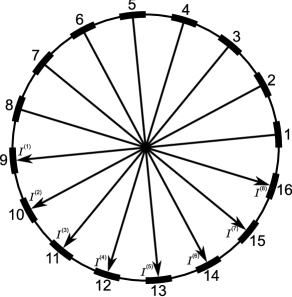
In order to study the effect of the prior model to the model reduction, we constructed the POD based reduced-order models corresponding to two different prior distributions. We denote the probability densities corresponding to the two priors by and . Both of the prior models were selected to be of the form of the proper (informative) smoothness prior [5, 21, 25]. In the two models, the variances of the nodal conductivity values were equal, . The degree of the spatial smoothness, however, differed between the two models; in the model , the cross-covariance decreased faster with the distance between the coordinates and than in the model . Five random samples corresponding to prior models and are depicted on top rows of Figures 2 and 3, respectively. As expected, the samples corresponding to are smoother than those corresponding to . On the bottom rows of Figures 2 and 3, the electric potential fields corresponding to the selected conductivity samples and the first current injection are illustrated.
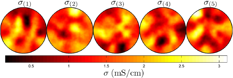
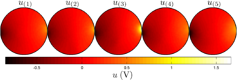
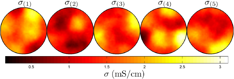
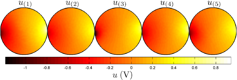
The POD modes corresponding to the priors and were constructed as described in Section 3. The sample sets consisted of 7500 conductivity and potential samples. In the selected test case, the current injections and prior distribution for the conductivity were rotationally symmetric. Hence, the POD basis for the potential was only generated corresponding to the first current injection ; the potential bases corresponding the other current injections were constructed by rotating the first basis by degrees. If the current injections or prior distribution were not rotationally symmetric, the POD basis would have been generated for each current injection separately. The first five POD bases of the conductivity and the potential corresponding to the prior models and are drawn in Figures 4 and 5, respectively. As expected, the POD bases of the conductivity are spatially smoother in the case of prior than in the case of prior . The POD bases of the potential possess qualitatively similar features in cases of the two different prior models.


The fractions of the variances that are captured by using - and -order approximations of and , respectively, are given by and . Figure 6 displays and for both prior models and . A rapid convergence of the retained variance fraction to 1 indicates that an accurate POD approximation requires only a small number of POD bases. Clearly, in the case of prior , the retained variance fraction increases more rapidly than in the case of prior . This result is intuitively appealing: when a random field features a very high spatial smoothness (prior model ), its variations can be represented in a low dimensional basis. For the same reason, increases more rapidly than – indeed, the samples of the electric potential are spatially much smoother than the samples of the conductivity (cf. Figs. 2 and 3). Further, the properties of are reflected by the smoothness of via the diffusion model (1); the smoother is, the smoother is also . In consequence, increases more rapidly in the case of prior than in the case of prior .
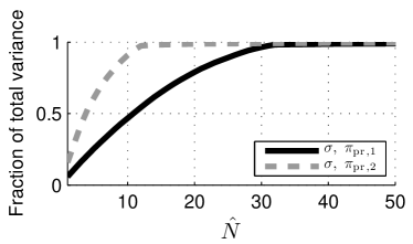
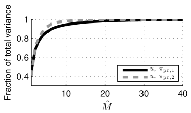
In this section, we demonstrated the effect of the prior model to the POD based model reduction by illustrating the samples, POD bases and retained variance fractions in cases of to two prior models and corresponding to different degrees or spatial smoothness. Below, we evaluate the POD based EIT reconstruction. The MAP estimates for the conductivity distributions are computed only using the prior model , that assumes higher spatial variation for the conductivity.
4.2 Simulation results
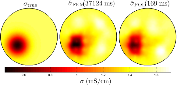
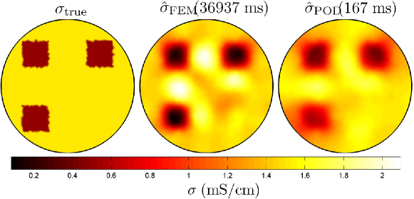
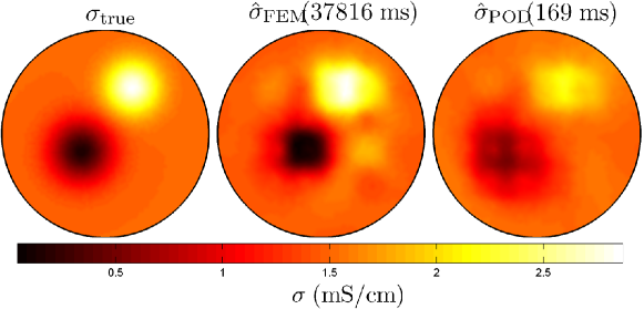
The simulation tests were carried out with three different target distributions: a target with a smooth resistive inclusion (test case 1), a target with three rectangular resistive inclusions with sharp boundaries (test case 2), and a target with both a resistive and a conductive inclusion (test case 3). The targets are illustrated in Figures 7-9 (left).
The simulated measurement data were computed using the conventional FE approximation of the measurement model. The FE mesh consisted of 8394 elements. The conductivity distribution was approximated in piecewise linear basis and the potential distribution in piecewise quadratic basis. The number of nodes in the 1st order FE mesh was 4374 and in the 2nd order mesh 17141. Gaussian distributed noise was added to the simulated measurements. The noise consists of two components: both of the components were of zero mean; the standard deviation (std) of the first component was 1% of the absolute value of the noiseless voltages, and the std of the second component was 0.1% of the difference between the maximum and minimum voltages.
The EIT reconstructions with both the conventional FE approximations and the POD based model reduction were computed. In the former case, the reconstruction was computed by solving the minimization problem (23), and in the latter case by solving (39). Both optimization problems were solved with the Gauss-Newton method, employed with a line-search [46]. The same prior model (see Section 4.1) was used both in conventional and in the reduced-order reconstructions. Further, in both cases, the variance of the measurement noise was assumed to be known. The numbers of POD modes both for and were selected such that of the variances of the respective random variables were retained. This yielded reduced-order representations consisting of 54 basis vectors for the conductivity and 25 basis vectors for the potential.
The reconstructions corresponding to both the conventional and the reduced-order model are depicted in Figures 7-9 (middle and right). The times required for each reconstruction are also indicated in the figures. In test case 1, the position of the inclusion was well tracked in both reconstructions. The computation time for the reconstruction corresponding to the conventional model was about 37 s, and for the reconstruction with the reduced-order model significantly less, below 200 milliseconds. That is, the reconstruction times were more than two orders of magnitude smaller in the case of the reduced-order model. In test cases 2 and 3, the reconstruction times were approximately the same as in test case 1. Also in these test cases, both standard and reduced-order reconstructions correspond well to the true targets. In all test cases, the POD-based reconstructions are only slighly smoother than those based on standard FE bases.
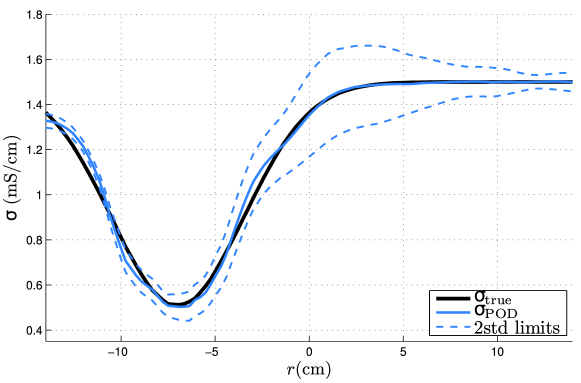
In test case 1, the reliability of the POD based reconstruction was assessed by computing the confidence limits defined by two standard deviations (std) for the reconstructed conductivity. The profiles of the true and the reconstructed conductivities, and the 2 std limits on a cross-section of the target domain are plotted in Figure 10. Here, we selected the cross-section such that it diagonally passes through the midpoints of the inclusion and the center of the circular target domain. The figure shows that the true conductivity is mostly between the 2 std limits. The figure also reveals that the uncertainty of the estimate is lowest near the target boundaries and the highest in the middle of the target. This is because the sensitivity of EIT measurements is highest near the target boundary where the electrodes are attached.
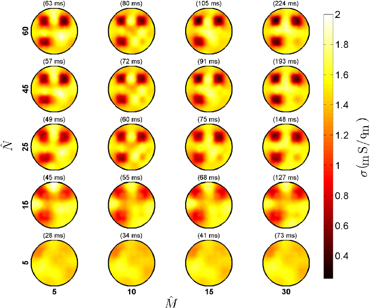
To study the effects of dimensions and of the POD bases and to reduced-order reconstructions, we computed the MAP estimates (39) corresponding to test case 2 using various choices of and . In Figure 11, the results are presented in the form of a table where increases from bottom to top, and increases from left to right. The computation times are written above the corresponding reconstructions. The results demonstrate that especially the number of basis functions for the potential () can be set very small without ruining the quality of the reconstructions – even the reconstructions with are relatively good, given that is large enough (). Clearly, the number of basis functions required for approximation the conductivity () is higher than that of potential – the reconstructions corresponding to are severely blurred. These are expected results, because with the selected prior model the number of basis functions required for retaining essentially all variations of is , while retaining the variations of requires somewhat less basis functions, cf. Figure 6.
4.3 Experimental results
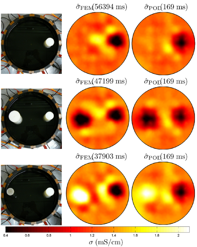
In the experiments, a cylindrical tank was filled with tap water, and three different target conductivities were constructed by inserting both resistive and conductive objects into the tank. The first target included one plastic (resistive) bar, the second target two plastic bars, and the third target contained one plastic and one metallic bar. All these inclusions were homogeneous in the vertical direction. Photos of all three targets are shown in the left column of Figure 12. The diameter of the tank was 28 cm and the height of the water level was 7 cm. The electrode configuration in the tank consisted of 16 uniformly positioned, 25 mm wide boundary electrodes, and they extended vertically from bottom to height of the water level. In Figure 12, the brown stripes on the tank wall indicate the locations of the electrodes. The measurements were carried out using opposite current injection scheme as in the simulations. As the measurement system, the SIPFIN measurement device was used 111SIPFIN is a modification of the Radic Research SIP256 instrument, see http://www.radic-research.de.
Again, the EIT reconstructions were computed both based on a conventional FE approximation of the CEM and with the POD reduced-order model. Same models were used as in the reconstructions based on simulated data in the previous section. The same numbers of POD basis functions were selected as in simulations studies with targets 1-3, i.e. and .
The results are shown in Figure 12. In the reconstructions, both corresponding to the conventional FE approximation of the CEM and the POD reduced-order model, the inclusions are clearly visible and the positions of the inclusions correspond to the real targets. In all test cases, the qualities of the reconstructions corresponding to the POD reduced-order model are comparable to those corresponding to the conventional FE based model. Again, the computation times were remarkably shorter when reduced-order model was used: with the conventional FE approximation, the computation times varied between 37903 ms and 56394 ms, while with the POD approximations the computations took only 169 ms in all test cases.
Some artifacts are present in all reconstuctions. These are due to 1) modeling errors that were not accounted for in the observation model. Such modeling errors are the discretization error and the error resulting from the unknown contact impedances. These errors could be accounted for by the approximation error modeling [21, 32, 33]. 2) Secondly, the selected prior model, the smoothness prior, is obviously not the best possible choice in the test cases. Indeed, accross the boundaries of the inclusions, the conductivity is discontinuous, and the conductivity contrasts are high. In such cases the assumption of smoothness is not a feasible one. However, as the aim of this study was only to demonstrate the feasibility of the POD based model reduction, we omit the considerations of other modeling errors and prior models from this paper.
5 CONCLUSIONS
In this paper, a reduced-order model for EIT has been proposed. The model is based on the POD representations of the electric conductivity distribution and the potential distribution. The model reduction is considered in the Bayesian inversion framework, and the POD bases are constructed based on a priori information on the conductivity. In the reconstructions, the errors caused by the model reduction are treated with the approximation error method. The reduced-order measurement model has been tested both simulated simulated and experimental data. The results show that by expressing the conductivity and the potential with reduced-order basis representation, it is possible to obtain feasible reconstructions with a low computational effort. In the selected test cases, the speedup was more than two orders of magnitude. In this paper, the POD based model reduction was tested with 2D examples. However, the proposed method can be directly implemented to computational 3D model of CEM in the presented form.
References
References
- [1] H.T. Banks, M.L. Joyner, B. Wincheski, and W.P. Winfree. Nondestructive evaluation using a reduced-order computational methodology. Inverse Problems, 16:929–945, 2000.
- [2] H.T. Banks and G.M. Kepler. Reduced order computational methods for electromagnetic material interrogation using pulsed signals and conductive reflecting interfaces. Journal of Inverse and Ill-posed Problems, 11:343–370, 2003.
- [3] D.C. Barber and B.H. Brown. Applied potential tomography. J Phys E: Sci Instrum, 17:723–733, 1984.
- [4] P. Brunet, R. Clement, and C. Bouvier. Monitoring soil water content and deficit using Electrical Resistivity Tomography (ERT) - A case study in the Cevennes area, France. Journal of Hydrology, 380(1-2):146–153, 2010.
- [5] D. Calvetti, J.P. Kaipio, and E. Somersalo. Aristotelian prior boundary conditions. Int. J. Math. Comp. Sci., 1:63–81, 2006.
- [6] Y. Cao, J. Zhu, Z. Luo, and I.M. Navon. Reduced-order modeling of the upper tropical pacific ocean model using proper orthogonal decomposition. Computers & Mathematics with Applications, 52(8-9):1373–1386, 2006.
- [7] K.-S. Cheng, D. Isaacson, J.C. Newell, and D.G. Gisser. Electrode models for electric current computed tomography. IEEE Trans Biomed Eng, 36:918–924, 1989.
- [8] AE Deane, IG Kevrekidis, GE Karniadakis, and SA Orszag. Low-dimensional models for complex geometry flows: Application to grooved channels and circular cylinders. Phys. Fluids A, 3:2337–2354, 1991.
- [9] B.A. Draper, K. Baek, M.S. Bartlett, and J.R. Beveridge. Recognizing faces with PCA and ICA. Computer vision and image understanding, 91(1-2):115–137, 2003.
- [10] I. Frerichs. Electrical impedance tomography (EIT) in applications related to lung and ventilation: a review of experimental and clinical activities. Physiological measurement, 21(2):R1–R21, 2000.
- [11] G. Göktürkler, C. Balkaya, and Z. Erhan. Geophysical investigation of a landslide: The Altindag landslide site, Izmir (western Turkey). Journal of Applied Geophysics, 65(2):84–96, 2008.
- [12] J.A. Gutierrez, T. Dyakowski, M.S. Beck, and R.A. Williams. Using electrical impedance tomography for controlling hydrocyclone underflow discharge. Powder Technology, 108(2-3):180–184, 2000.
- [13] J. Heino, E. Somersalo, and J.P. Kaipio. Compensation for geometric mismodelling by anisotropies in optical tomography. Opt. Exp., 13:296–308, 2005.
- [14] P Holmes, JL Lumley, and G Berkooz. Turbulence, coherent structures, dynamical systems and symmetry. Cambridge University Press, 1998.
- [15] S. Hosseini, D. Patel, F. Ein-Mozaffari, and M. Mehrvar. Study of solid-liquid mixing in agitated tanks through electrical resistance tomography. Chemical Engineering Science, 65(4):1374–1384, 2010.
- [16] H. Hotelling. Analysis of a complex of statistical variables into principal components. J. Educ. Psychol., 24:417–441, 1933.
- [17] B. Jin. Fast Bayesian approach for parameter estimation. International Journal for Numerical Methods in Engineering, 76:230–252, 2008.
- [18] I.T. Jolliffe. Principal Component Analysis. Springer-Verlag, 2002.
- [19] J.P. Kaipio, V. Kolehmainen, E. Somersalo, and M. Vauhkonen. Statistical inversion and Monte Carlo sampling methods in electrical impedance tomography. Inverse Problems, 16:1487–1522, 2000.
- [20] J.P. Kaipio, V. Kolehmainen, M. Vauhkonen, and E. Somersalo. Inverse problem with structural prior information. Inverse Problems, 15(3):713–729, 1999.
- [21] J.P. Kaipio and E. Somersalo. Statistical and Computational Inverse Problems. Springer New York, 2005.
- [22] J.P. Kaipio and E. Somersalo. Statistical inverse problems: discretization, model reduction and inverse crimes. Journal of Computational and Applied Mathematics, 198(2):493–504, 2007.
- [23] K. Karhunen. Uber Lineare Methoden in der Wahrscheinlichkeitsrechnung. Annales Academiae Sciientiarum Fennicae, Series AI: Mathematica-Physica, 37:3–79, 1946.
- [24] M. Kirby and L. Sirovich. Application of the Karhunen-Loeve procedure for the characterization of human faces. IEEE Transactions on Pattern Analysis and Machine Intelligence, 12(1):103–108, 1990.
- [25] V. Kolehmainen, J.P. Kaipio, and H.R.B. Orlande. Reconstruction of thermal conductivity and heat capacity using a tomographic approach. International journal of heat and mass transfer, 50(25-26):5150–5160, 2007.
- [26] V. Kolehmainen, T. Tarvainen, S.R. Arridge, and J.P. Kaipio. Marginalization of uninteresting distributed parameters in inverse problems - application to optical tomography. Int J Uncertainty Quantification, 1:1–17, 2011.
- [27] A. Lehikoinen, S. Finsterle, A. Voutilainen, L.M. Heikkinen, M. Vauhkonen, and J.P. Kaipio. Approximation errors and truncation of computational domains with application to geophysical tomography. Inverse Problems and Imaging, 1(2):371–389, 2007.
- [28] C. Lieberman, K. Willcox, and O. Ghattas. Parameter and state model reduction for large-scale statistical inverse problems. SIAM Journal on Scientific Computing, 32:2523–2542, 2010.
- [29] M. Lòeve. Fonctions aléatoires de second ordre. Rev. Sci., pages 195–206, 1946.
- [30] M. Lòeve. Probability Theory. Princeton, N.J.: Van Nostrand, 1955.
- [31] X. Ma and G. Karniadakis. A low-dimensional model for simulating three-dimensional cylinder flow. J. Fluid Mech., 458:181–190, 2002.
- [32] A. Nissinen, L.M. Heikkinen, and J.P. Kaipio. The Bayesian approximation error approach for electrical impedance tomography experimental results. Meas. Sci. Technol., 19:015501 (9pp), 2008.
- [33] A. Nissinen, L.M. Heikkinen, V. Kolehmainen, and J.P. Kaipio. Compensation of errors due to discretization, domain truncation and unknown contact impedances in electrical impedance tomography. Meas. Sci. Technol., 20:105504 (13pp), 2009.
- [34] L. Pakzad, F. Ein-Mozaffari, and P. Chan. Using electrical resistance tomography and computational fluid dynamics modeling to study the formation of cavern in the mixing of pseudoplastic fluids possessing yield stress. Chemical Engineering Science, 63:2508–2522, 2008.
- [35] B.-G. Park, J.-H. Moon, B.-S. Lee, and S. Kim. An electrical resistance tomography technique for the monitoring of a radioactive waste separation process. International Communications in Heat and Mass Transfer, 35(10):1307–1310, 2008.
- [36] A. Perrone, A. Ianuzzi, V. Lapenna, P. Lorenzo, S. Piscitelli, E. Rizzo, and F. Sdao. High-resolution electrical imaging of the Carco d’Izzo earthflow (southern Italy). Journal of Applied Geophysics, 56(1):17–29, 2004.
- [37] S. Pursiainen. Two-stage reconstruction of a circular anomaly in electrical impedance tomography. Inverse Problems, 22:1689–1703, 2006.
- [38] S. Pursiainen and H. Hakula. A high-order finite element method for electrical impedance tomography. In Progress In Electromagnetics Research Symposium 2006, Cambridge, USA, pages 260–264, 2006.
- [39] S.S. Ravindran. A reduced-order approach for optimal control of fluids using proper orthogonal decomposition. International Journal for Numerical Methods in Fluids, 34(5):425–448, 2000.
- [40] F. Santosa and M. Vogelius. A backprojection algorithm for electrical impedance imaging. SIAM J Appl Math, 50:216–243, 1990.
- [41] L. Sirovich and M. Kirby. Low-dimensional procedure for the characterization of human faces. Journal of the Optical Society of America A, 4(3):519–524, 1987.
- [42] E. Somersalo, M. Cheney, and D. Isaacson. Existence and uniqueness for electrode models for electric current computed tomography. SIAM J Appl Math, 52:1023–1040, 1992.
- [43] M.S. Takriff, A.A. Hamzah, S.K. Kamarudin, and J. Abdullah. Electrical resistance tomography investigation of gas dispersion in gas-liquid mixing in an agitated vessel. Journal of Applied Sciences, 9(17):3110–3115, 2009.
- [44] M. Vauhkonen, J.P. Kaipio, E. Somersalo, and P.A. Karjalainen. Electrical impedance tomography with basis constraints. Inverse Problems, 13:523–530, 1997.
- [45] P.J. Vauhkonen, M. Vauhkonen, T. Savolainen, and J.P. Kaipio. Three-dimensional electrical impedance tomography based on the complete electrode model. IEEE Transactions on Biomedical Engineering, 46:1150–1160, 1999.
- [46] P.J. Vauhkonen, M. Vauhkonen, A. Seppänen, and Kaipio J.P. Iterative image reconstruction in three-dimensional electrical impedance tomography. In Proc. Inverse Problems, Design and Optimization Symposium, Rio de Janeiro, Brazil, 2004.
- [47] T. Vilhunen, J.P. Kaipio, P.J. Vauhkonen, T. Savolainen, and M. Vauhkonen. Simultaneous reconstruction of electrode contact impedances and internal electrical properties. Part I: Theory. Meas. Sci. Technol., 13:1848–1854, 2002.
- [48] R.A. Williams and M.S. Beck, editors. Process Tomography, Principles, Techniques and Applications. Oxford: Butterworth-Heinemann, 1995.
- [49] R.A. Williams, F.J. Dickin, J.A. Gutierrez, T. Dyakowski, and M.S. Beck. Using electrical impedance tomography for controlling hydrocyclone underflow discharge. Control Engineering Practice, 5(2):253–256, 1997.
- [50] K.Y. Yeung and W.L. Ruzzo. Principal component analysis for clustering gene expression data. Bioinformatics, 17(9):763–774, 2001.
- [51] L. Zhang, W. Dong, D. Zhang, and G. Shi. Two-stage image denoising by principal component analysis with local pixel grouping. Pattern Recognition, 43:1531–1549, 2009.
- [52] Y. Zou and Z. Guo. A review of electrical impedance techniques for breast cancer detection. Medical engineering & physics, 25(2):79–90, 2003.