Poisoning Attacks against Support Vector Machines

Abstract

We investigate a family of poisoning attacks against Support Vector Machines (SVM). Such attacks inject specially crafted training data that increases the SVM’s test error. Central to the motivation for these attacks is the fact that most learning algorithms assume that their training data comes from a natural or well-behaved distribution. However, this assumption does not generally hold in security-sensitive settings. As we demonstrate, an intelligent adversary can, to some extent, predict the change of the SVM’s decision function due to malicious input and use this ability to construct malicious data.

The proposed attack uses a gradient ascent strategy in which the gradient is computed based on properties of the SVM’s optimal solution. This method can be kernelized and enables the attack to be constructed in the input space even for non-linear kernels. We experimentally demonstrate that our gradient ascent procedure reliably identifies good local maxima of the non-convex validation error surface, which significantly increases the classifier’s test error.

1 Introduction

Machine learning techniques are rapidly emerging as a vital tool in a variety of networking and large-scale system applications because they can infer hidden patterns in large complicated datasets, adapt to new behaviors, and provide statistical soundness to decision-making processes. Application developers thus can employ learning to help solve so-called big-data problems and these include a number of security-related problems particularly focusing on identifying malicious or irregular behavior. In fact, learning approaches have already been used or proposed as solutions to a number of such security-sensitive tasks including spam, worm, intrusion and fraud detection (Meyer & Whateley, 2004; Biggio et al., 2010; Stolfo et al., 2003; Forrest et al., 1996; Bolton & Hand, 2002; Cova et al., 2010; Rieck et al., 2010; Curtsinger et al., 2011; Laskov & Šrndić, 2011). Unfortunately, in these domains, data is generally not only non-stationary but may also have an adversarial component, and the flexibility afforded by learning techniques can be exploited by an adversary to achieve his goals. For instance, in spam-detection, adversaries regularly adapt their approaches based on the popular spam detectors, and generally a clever adversary will change his behavior either to evade or mislead learning.

In response to the threat of adversarial data manipulation, several proposed learning methods explicitly account for certain types of corrupted data (Globerson & Roweis, 2006; Teo et al., 2008; Brückner & Scheffer, 2009; Dekel et al., 2010). Attacks against learning algorithms can be classified, among other categories (c.f. Barreno et al., 2010), into causative (manipulation of training data) and exploratory (exploitation of the classifier). Poisoning refers to a causative attack in which specially crafted attack points are injected into the training data. This attack is especially important from the practical point of view, as an attacker usually cannot directly access an existing training database but may provide new training data; e.g., web-based repositories and honeypots often collect malware examples for training, which provides an opportunity for the adversary to poison the training data. Poisoning attacks have been previously studied only for simple anomaly detection methods (Barreno et al., 2006; Rubinstein et al., 2009; Kloft & Laskov, 2010).

In this paper, we examine a family of poisoning attacks against Support Vector Machines (SVM). Following the general security analysis methodology for machine learning, we assume that the attacker knows the learning algorithm and can draw data from the underlying data distribution. Further, we assume that our attacker knows the training data used by the learner; generally, an unrealistic assumption, but in real-world settings, an attacker could instead use a surrogate training set drawn from the same distribution (e.g., Nelson et al., 2008) and our approach yields a worst-case analysis of the attacker’s capabilities. Under these assumptions, we present a method that an attacker can use to construct a data point that significantly decreases the SVM’s classification accuracy.

The proposed method is based on the properties of the optimal solution of the SVM training problem. As was first shown in an incremental learning technique (Cauwenberghs & Poggio, 2001), this solution depends smoothly on the parameters of the respective quadratic programming problem and on the geometry of the data points. Hence, an attacker can manipulate the optimal SVM solution by inserting specially crafted attack points. We demonstrate that finding such an attack point can be formulated as optimization with respect to a performance measure, subject to the condition that an optimal solution of the SVM training problem is retained. Although the test error surface is generally nonconvex, the gradient ascent procedure used in our method reliably identifies good local maxima of the test error surface.

The proposed method only depends on the gradients of the dot products between points in the input space, and hence can be kernelized. This contrasts previous work involving construction of special attack points (e.g., Brückner & Scheffer, 2009; Kloft & Laskov, 2010) in which attacks could only be constructed in the feature space for the nonlinear case. The latter is a strong disadvantage for the attacker, since he must construct data in the input space and has no practical means to access the feature space. Hence, the proposed method breaks new ground in optimizing the impact of data-driven attacks against kernel-based learning algorithms and emphasizes the need to consider resistance against adversarial training data as an important factor in the design of learning algorithms.

2 Poisoning attack on SVM

We assume the SVM has been trained on a data set $\mathcal{D}_{\text{tr}}=\{x_{i},y_{i}\}_{i=1}^{n}$, $x_{i}\in\mathbb{R}^{d}$. Following the standard notation, $K$ denotes the matrix of kernel values between two sets of points, $Q=yy^{\top}\odot K$ denotes the label-annotated version of $K$, and $\alpha$ denotes the SVM’s dual variables corresponding to each training point. Depending on the value of $\alpha_{i}$, the training points are referred to as margin support vectors ($0<\alpha_{i}<C$, set $\mathcal{S}$), error support vectors ($\alpha_{i}=C$, set $\mathcal{E}$) and reserve points ($\alpha_{i}=0$, set $\mathcal{R}$). In the sequel, the lower-case letters $s,e,r$ are used to index the corresponding parts of vectors or matrices; e.g., $Q_{ss}$ denotes the margin support vector submatrix of $Q$.

2.1 Main derivation

For a poisoning attack, the attacker’s goal is to find a point $(x_{c},y_{c})$, whose addition to $\mathcal{D}_{\text{tr}}$ maximally decreases the SVM’s classification accuracy. The choice of the attack point’s label, $y_{c}$, is arbitrary but fixed. We refer to the class of this chosen label as attacking class and the other as the attacked class.

The attacker proceeds by drawing a validation data set $\mathcal{D}_{\text{val}}=\{x_{k},y_{k}\}_{k=1}^{m}$ and maximizing the hinge loss incurred on $\mathcal{D}_{\text{val}}$ by the SVM trained on $\mathcal{D}_{\text{tr}}\cup(x_{c},y_{c})$:

$$\max_{x_{c}}L(x_{c})=\sum_{k=1}^{m}(1-y_{k}f_{x_{c}}(x_{k}))_{+}=\sum_{k=1}^{m}(-g_{k})_{+}\enspace$$ (1)

In this section, we assume the role of the attacker and develop a method for optimizing $x_{c}$ with this objective.

First, we explicitly account for all terms in the margin conditions $g_{k}$ that are affected by $x_{c}$:

$$g_{k} =\sum_{j}Q_{kj}\alpha_{j}+y_{k}b-1$$ (2)

$$=\sum_{j\neq c}Q_{kj}\alpha_{j}(x_{c})+Q_{kc}(x_{c})\alpha_{c}(x_{c})+y_{k}b(x_{c})-1\;.$$

It is not difficult to see from the above equations that $L(x_{c})$ is a non-convex objective function. Thus, we exploit a gradient ascent technique to iteratively optimize it. We assume that an initial location of the attack point $x_{c}^{(0)}$ has been chosen. Our goal is to update the attack point as $x_{c}^{(p)}=x_{c}^{(p-1)}+tu$ where $p$ is the current iteration, $u$ is a norm-1 vector representing the attack direction, and $t$ is the step size. Clearly, to maximize our objective, the attack direction $u$ aligns to the gradient of $L$ with respect to $u$, which has to be computed at each iteration.

Although the hinge loss is not everywhere differentiable, this can be overcome by only considering point indices $k$ with non-zero contributions to $L$; i.e., those for which $-g_{k}>0$. Contributions of such points to the gradient of $L$ can be computed by differentiating Eq. (2) with respect to $u$ using the product rule:

$$\frac{\partial g_{k}}{\partial u}=Q_{ks}\frac{\partial\alpha}{\partial u}+\frac{\partial Q_{kc}}{\partial u}\alpha_{c}+y_{k}\frac{\partial b}{\partial u},$$ (3)

where

$$\frac{\partial\alpha}{\partial u}=\begin{bmatrix}\frac{\partial\alpha_{1}}{\partial u_{1}}&\cdots&\frac{\partial\alpha_{1}}{\partial u_{d}}\\ \vdots&\ddots&\vdots\\ \frac{\partial\alpha_{s}}{\partial u_{1}}&\cdots&\frac{\partial\alpha_{s}}{\partial u_{d}}\end{bmatrix},\;\text{simil.}\;\frac{\partial Q_{kc}}{\partial u},\,\frac{\partial b}{\partial u}\enspace.$$

The expressions for the gradient can be further refined using the fact that the step taken in direction $u$ should maintain the optimal SVM solution. This can expressed as an adiabatic update condition using the technique introduced in (Cauwenberghs & Poggio, 2001). Observe that for the $i$-th point in the training set, the KKT conditions for the optimal solution of the SVM training problem can be expressed as:

$$g_{i} =\sum_{j\in\mathcal{D}_{\text{tr}}}Q_{ij}\alpha_{j}+y_{i}b-1\begin{cases}>0;\;i\in\mathcal{R}\\ =0;\;i\in\mathcal{S}\\ <0;\;i\in\mathcal{E}\end{cases}$$ (4)

$$h =\sum_{j\in\mathcal{D}_{\text{tr}}}y_{j}\alpha_{j}=0\enspace.$$ (5)

The equality in condition (4) and (5) implies that an infinitesimal change in the attack point $x_{c}$ causes a smooth change in the optimal solution of the SVM, under the restriction that the composition of the sets $\mathcal{S}$, $\mathcal{E}$ and $\mathcal{R}$ remain intact. This equilibrium allows us to predict the response of the SVM solution to the variation of $x_{c}$, as shown below.

By differentiation of the $x_{c}$-dependent terms in Eqs. (4)–(5) with respect to each component $u_{l}$ ($1\leq l\leq d$), we obtain, for any $i\in\mathcal{S}$,

$$\frac{\partial g}{\partial u_{l}} =Q_{ss}\frac{\partial\alpha}{\partial u_{l}}+\frac{\partial Q_{sc}}{\partial u_{l}}\alpha_{c}+y_{s}\frac{\partial b}{\partial u_{l}}=0$$ (6)

$$\frac{\partial h}{\partial u_{l}} =y_{s}^{\top}\frac{\partial\alpha}{\partial u_{l}}=0\enspace,$$

which can be rewritten as

$$\begin{bmatrix}\frac{\partial b}{\partial u_{l}}\\ \frac{\partial\alpha}{\partial u_{l}}\end{bmatrix} =-{\begin{bmatrix}0&y_{S}^{\top}\\ y_{s}&Q_{ss}\end{bmatrix}}^{-1}\begin{bmatrix}0\\ \frac{\partial Q_{sc}}{\partial u_{l}}\end{bmatrix}\alpha_{c}\enspace.$$ (7)

The first matrix can be inverted using the Sherman-Morrison-Woodbury formula (Lütkepohl, 1996):

$$\begin{bmatrix}0&y_{s}^{\top}\\ y_{s}&Q_{ss}\end{bmatrix}^{-1}=\frac{1}{\zeta}\begin{bmatrix}-1&\upsilon^{\top}\\ \upsilon&\zeta Q_{ss}^{-1}-\upsilon\upsilon^{\top}\end{bmatrix}$$ (8)

where $\upsilon=Q_{ss}^{-1}y_{s}$ and $\zeta=y_{s}^{\top}Q_{ss}^{-1}y_{s}$. Substituting (8) into (7) and observing that all components of the inverted matrix are independent of $x_{c}$, we obtain:

$$\frac{\partial\alpha}{\partial u} =-\frac{1}{\zeta}\alpha_{c}(\zeta Q_{ss}^{-1}-\upsilon\upsilon^{\top})\cdot\frac{\partial Q_{sc}}{\partial u}$$ (9)

$$\frac{\partial b}{\partial u} =-\frac{1}{\zeta}\alpha_{c}\upsilon^{\top}\cdot\frac{\partial Q_{sc}}{\partial u}\enspace.$$

Substituting (9) into (3) and further into (1), we obtain the desired gradient used for optimizing our attack:

$$\frac{\partial L}{\partial u}=\sum_{k=1}^{m}\left\{M_{k}\frac{\partial Q_{sc}}{\partial u}+\frac{\partial Q_{kc}}{\partial u}\right\}\alpha_{c},$$ (10)

where

$$M_{k}=-\frac{1}{\zeta}(Q_{ks}(\zeta Q_{ss}^{-1}-\upsilon\upsilon^{T})+y_{k}\upsilon^{T}).$$

2.2 Kernelization

From Eq. (10), we see that the gradient of the objective function at iteration $k$ may depend on the attack point $x_{c}^{(p)}=x_{c}^{(p-1)}+tu$ only through the gradients of the matrix $Q$. In particular, this depends on the chosen kernel. We report below the expressions of these gradients for three common kernels.

• Linear kernel:

  $$\frac{\partial K_{ic}}{\partial u}=\frac{\partial(x_{i}\cdot x_{c}^{(p)})}{\partial u}=tx_{i}$$

• Polynomial kernel:

  $$\frac{\partial K_{ic}}{\partial u}=\frac{\partial(x_{i}\cdot x_{c}^{(p)}+R)^{d}}{\partial u}=d(x_{i}\cdot x_{c}^{(p)}+R)^{d-1}tx_{i}$$

• RBF kernel:

  $$\frac{\partial K_{ic}}{\partial u}=\frac{\partial e^{-\frac{\gamma}{2}||x_{i}-x_{c}||^{2}}}{\partial u}=K(x_{i},x_{c}^{(p)})\gamma t(x_{i}-x_{c}^{(p)})$$

The dependence on $x_{c}^{(p)}$ (and, thus, on $u$) in the gradients of non-linear kernels can be avoided by substituting $x_{c}^{(p)}$ with $x_{c}^{(p-1)}$, provided that $t$ is sufficiently small. This approximation enables a straightforward extension of our method to arbitrary kernels.

2.3 Poisoning Attack Algorithm

The algorithmic details of the method described in Section 2.1 are presented in Algorithm 1.

In this algorithm, the attack vector $x_{c}^{(0)}$ is initialized by cloning an arbitrary point from the attacked class and flipping its label. In principle, any point sufficiently deep within the attacking class’s margin can be used as a starting point. However, if this point is too close to the boundary of the attacking class, the iteratively adjusted attack point may become a reserve point, which halts further progress.

Algorithm 1 Poisoning attack against SVM

Input: $\mathcal{D}_{\rm tr}$, the training data; $\mathcal{D}_{\rm val}$, the validation data; $y_{c}$, the class label of the attack point; $x_{c}^{(0)}$, the initial attack point; $t$, the step size.
Output: $x_{c}$, the final attack point.

1:   $\{\alpha_{i},b\}\leftarrow$ learn an SVM on $\mathcal{D}_{\rm tr}$.

2:  $k\leftarrow 0$.

3:  repeat

4:     Re-compute the SVM solution on $\mathcal{D}_{\rm tr}\cup\{x_{c}^{(p)},y_{c}\}$ using incremental SVM (e.g., Cauwenberghs & Poggio, 2001). This step requires $\{\alpha_{i},b\}$.

5:     Compute $\frac{\partial L}{\partial u}$ on $\mathcal{D}_{\rm val}$ according to Eq. (10).

6:     Set $u$ to a unit vector aligned with $\frac{\partial L}{\partial u}$.

7:     $k\leftarrow k+1$ and $x_{c}^{(p)}\leftarrow x_{c}^{(p-1)}+tu$

8:  until $L\left(x_{c}^{(p)}\right)-L\left(x_{c}^{(p-1)}\right)<\epsilon$

9:  return: $x_{c}=x_{c}^{(p)}$

The computation of the gradient of the validation error crucially depends on the assumption that the structure of the sets $\mathcal{S}$, $\mathcal{E}$ and $\mathcal{R}$ does not change during the update. In general, it is difficult to determine the largest step $t$ along an arbitrary direction $u$, which preserves this structure. The classical line search strategy used in gradient ascent methods is not suitable for our case, since the update to the optimal solution for large steps may be prohibitively expensive. Hence, the step $t$ is fixed to a small constant value in our algorithm. After each update of the attack point $x_{c}^{(p)}$, the optimal solution is efficiently recomputed from the solution on $\mathcal{D}_{\rm tr}$, using the incremental SVM machinery (e.g., Cauwenberghs & Poggio, 2001).

The algorithm terminates when the change in the validation error is smaller than a predefined threshold. For kernels including the linear kernel, the surface of the validation error is unbounded, hence the algorithm is halted when the attack vector deviates too much from the training data; i.e., we bound the size of our attack points.

3 Experiments

The experimental evaluation presented in the following sections demonstrates the behavior of our proposed method on an artificial two-dimensional dataset and evaluates its effectiveness on the classical MNIST handwritten digit recognition dataset.

3.1 Artificial data

We first consider a two-dimensional data generation model in which each class follows a Gaussian distribution with mean and covariance matrices given by $\mu_{-}=[-1.5,0]$, $\mu_{+}=[1.5,0]$, $\Sigma_{-}=\Sigma_{+}=0.6I$. The points from the negative distribution are assigned the label $-1$ (shown as red in the subsequent figures) and otherwise $+1$ (shown as blue). The training and the validation sets, $\mathcal{D}_{\rm tr}$ and $\mathcal{D}_{\rm val}$ (consisting of $25$ and $500$ points per class, respectively) are randomly drawn from this distribution.

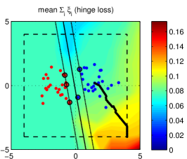
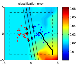
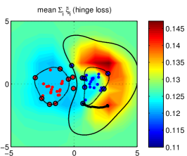
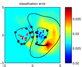
In the experiment presented below, the red class is the attacking class. To this end, a random point of the blue class is selected and its label is flipped to serve as the starting point for our method. Our gradient ascent method is then used to refine this attack until its termination condition is satisfied. The attack’s trajectory is traced as the black line in Fig. 1 for both the linear kernel (upper two plots) and the RBF kernel (lower two plots). The background in each plot represents the error surface explicitly computed for all points within the box $x\in[-5,5]^{2}$. The leftmost plots in each pair show the hinge loss computed on a validation set while the rightmost plots in each pair show the classification error for the area of interest. For the linear kernel, the range of attack points is limited to the box $x\in[-4,4]^{2}$ shown as a dashed line.

For both kernels, these plots show that our gradient ascent algorithm finds a reasonably good local maximum of the non-convex error surface. For the linear kernel, it terminates at the corner of the bounded region, since the error surface is unbounded. For the RBF kernel, it also finds a good local maximum of the hinge loss which, incidentally, is the maximum classification error within this area of interest.

Figure 1: Behavior of the gradient-based attack strategy on the Gaussian data sets, for the linear (top row) and the RBF kernel (bottom row) with $\gamma=0.5$. The regularization parameter $C$ was set to $1$ in both cases. The solid black line represents the gradual shift of the attack point $x_{c}^{(p)}$ toward a local maximum. The hinge loss and the classification error are shown in colors, to appreciate that the hinge loss provides a good approximation of the classification error. The value of such functions for each point $x\in[-5,5]^{2}$ is computed by learning an SVM on $\mathcal{D}_{\rm tr}\cup\{x,y=-1\}$ and evaluating its performance on $\mathcal{D}_{\rm val}$. The SVM solution on the clean data $\mathcal{D}_{\rm tr}$, and the training data itself, are reported for completeness, highlighting the support vectors (with black circles), the decision hyperplane and the margin bounds (with black lines).

3.2 Real data

We now quantitatively validate the effectiveness of the proposed attack strategy on a well-known MNIST handwritten digit classification task (LeCun et al., 1995). Similarly to Globerson & Roweis (2006), we focus on two-class sub-problems of discriminating between two distinct digits. In particular, we consider the following two-class problems: 7 vs. 1; 9 vs. 8; 4 vs. 0. The visual nature of the handwritten digit data provides us with a semantic meaning for an attack.

Each digit in the MNIST data set is properly normalized and represented as a grayscale image of $28\times 28$ pixels. In particular, each pixel is ordered in a raster-scan and its value is directly considered as a feature. The overall number of features is $d=28\times 28=784$. We normalized each feature (pixel value) $x\in[0,1]^{d}$ by dividing its value by $255$.

In this experiment only the linear kernel is considered, and the regularization parameter of the SVM is fixed to $C=1$. We randomly sample a training and a validation data of $100$ and $500$ samples, respectively, and retain the complete testing data given by MNIST for $\mathcal{D}_{\rm ts}$. Although it varies for each digit, the size of the testing data is about 2000 samples per class (digit).

Figure 2: Modifications to the initial (mislabeled) attack point performed by the proposed attack strategy, for the three considered two-class problems from the MNIST data set. The increase in validation and testing errors across different iterations is also reported.

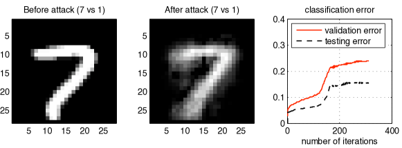
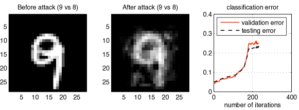
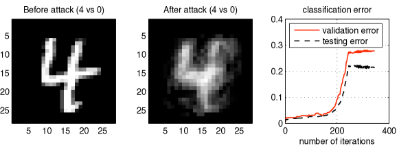
The results of the experiment are presented in Fig. 2. The leftmost plots of each row show the example of the attacked class taken as starting points in our algorithm. The middle plots show the final attack point. The rightmost plots displays the increase in the validation and testing errors as the attack progresses.

The visual appearance of the attack point reveals that the attack blurs the initial prototype toward the appearance of examples of the attacking class. Comparing the initial and final attack points, we see this effect: the bottom segment of the $7$ straightens to resemble a $1$, the lower segment of the $9$ becomes more round thus mimicking an $8$, and round noise is added to the outer boundary of the $4$ to make it similar to a $0$.

The increase in error over the course of attack is especially striking, as shown in the rightmost plots. In general, the validation error overestimates the classification error due to a smaller sample size. Nonetheless, in the exemplary runs reported in this experiment, a single attack data point caused the classification error to rise from the initial error rates of 2–5% to 15–20%. Since our initial attack point is obtained by flipping the label of a point in the attacked class, the errors in the first iteration of the rightmost plots of Fig. 2 are caused by single random label flips. This confirms that our attack can achieve significantly higher error rates than random label flips, and underscores the vulnerability of the SVM to poisoning attacks.

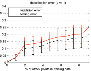
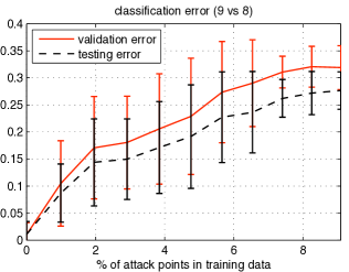
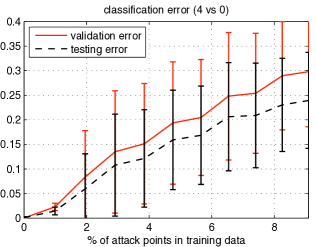
The latter point is further illustrated in a multiple point, multiple run experiment presented in Fig. 3. For this experiment, the attack was extended by injecting additional points into the same class and averaging results over multiple runs on randomly chosen training and validation sets of the same size (100 and 500 samples, respectively). One can clearly see a steady growth of the attack effectiveness with the increasing percentage of the attack points in the training set. The variance of the error is quite high, which can be explained by relatively small sizes of the training and validation data sets.

Figure 3: Results of the multi-point, multi-run experiments on the MNIST data set. In each plot, we show the classification errors due to poisoning as a function of the percentage of training contamination for both the validation (red solid line) and testing sets (black dashed line). The topmost plot is for the $7$ vs.$1$ classifier, the middle is for the $9$ vs. $8$ classifier, and the bottommost is for the $4$ vs. $0$ classifier.

4 Conclusions and Future Work

The poisoning attack presented in this paper is the first step toward the security analysis of SVM against training data attacks. Although our gradient ascent method is arguably a crude algorithmic procedure, it attains a surprisingly large impact on the SVM’s empirical classification accuracy. The presented attack method also reveals the possibility for assessing the impact of transformations carried out in the input space on the functions defined in the Reproducing Kernel Hilbert Spaces by means of differential operators. Compared to previous work on evasion of learning algorithms (e.g., Brückner & Scheffer, 2009; Kloft & Laskov, 2010), such influence may facilitate the practical realization of various evasion strategies. These implications need to be further investigated.

Several potential improvements to the presented method remain to be explored in future work. The first would be to address our optimization method’s restriction to small changes in order to maintain the SVM’s structural constraints. We solved this by taking many tiny gradient steps. It would be interesting to investigate a more accurate and efficient computation of the largest possible step that does not alter the structure of the optimal solution.

Another direction for research is the simultaneous optimization of multi-point attacks, which we successfully approached with sequential single-point attacks. The first question is how to optimally perturb a subset of the training data; that is, instead of individually optimizing each attack point, one could derive simultaneous steps for every attack point to better optimize their overall effect. The second question is how to choose the best subset of points to use as a starting point for the attack. Generally, the latter is a subset selection problem but heuristics may allow for improved approximations. Regardless, we demonstrate that even non-optimal multi-point attack strategies significantly degrade the SVM’s performance.

An important practical limitation of the proposed method is the assumption that the attacker controls the labels of the injected points. Such assumptions may not hold when the labels are only assigned by trusted sources such as humans. For instance, a spam filter uses its users’ labeling of messages as its ground truth. Thus, although an attacker can send arbitrary messages, he cannot guarantee that they will have the labels necessary for his attack. This imposes an additional requirement that the attack data must satisfy certain side constraints to fool the labeling oracle. Further work is needed to understand these potential side constraints and to incorporate them into attacks.

The final extension would be to incorporate the real-world inverse feature-mapping problem; that is, the problem of finding real-world attack data that can achieve the desired result in the learner’s input space. For data like handwritten digits, there is a direct mapping between the real-world image data and the input features used for learning. In many other problems (e.g., spam filtering) the mapping is more complex and may involve various non-smooth operations and normalizations. Solving these inverse mapping problems for attacks against learning remains open.

References

- Barreno et al. (2006) Barreno, Marco, Nelson, Blaine, Sears, Russell, Joseph, Anthony D., and Tygar, J. D. Can machine learning be secure? In Proceedings of the ACM Symposium on Information, Computer and Communications Security (ASIACCS), pp. 16–25, 2006.
- Barreno et al. (2010) Barreno, Marco, Nelson, Blaine, Joseph, Anthony D., and Tygar, J. D. The security of machine learning. Machine Learning, 81(2):121–148, November 2010.
- Biggio et al. (2010) Biggio, Battista, Fumera, Giorgio, and Roli, Fabio. Multiple classifier systems for robust classifier design in adversarial environments. International Journal of Machine Learning and Cybernetics, 1(1):27–41, 2010.
- Bolton & Hand (2002) Bolton, Richard J. and Hand, David J. Statistical fraud detection: A review. Journal of Statistical Science, 17(3):235–255, 2002.
- Brückner & Scheffer (2009) Brückner, Michael and Scheffer, Tobias. Nash equilibria of static prediction games. In Advances in Neural Information Processing Systems (NIPS), pp. 171–179. 2009.
- Cauwenberghs & Poggio (2001) Cauwenberghs, Gert and Poggio, Tomaso. Incremental and decremental support vector machine learning. In Leen, T.K., Diettrich, T.G., and Tresp, V. (eds.), Advances in Neural Information Processing Systems 13, pp. 409–415, 2001.
- Cova et al. (2010) Cova, M., Kruegel, C., and Vigna, G. Detection and analysis of drive-by-download attacks and malicious JavaScript code. In International Conference on World Wide Web (WWW), pp. 281–290, 2010.
- Curtsinger et al. (2011) Curtsinger, C., Livshits, B., Zorn, B., and Seifert, C. ZOZZLE: Fast and precise in-browser JavaScript malware detection. In USENIX Security Symposium, pp. 33–48, 2011.
- Dekel et al. (2010) Dekel, O., Shamir, O., and Xiao, L. Learning to classify with missing and corrupted features. Machine Learning, 81(2):149–178, 2010.
- Forrest et al. (1996) Forrest, Stephanie, Hofmeyr, Steven A., Somayaji, Anil, and Longstaff, Thomas A. A sense of self for unix processes. In Proceedings of the IEEE Symposium on Security and Privacy, pp. 120–128, 1996.
- Globerson & Roweis (2006) Globerson, A. and Roweis, S. Nightmare at test time: Robust learning by feature deletion. In International Conference on Machine Learning (ICML), pp. 353–360, 2006.
- Kloft & Laskov (2010) Kloft, Marius and Laskov, Pavel. Online anomaly detection under adversarial impact. In Proceedings of the 13th International Conference on Artificial Intelligence and Statistics (AISTATS), 2010.
- Laskov & Šrndić (2011) Laskov, Pavel and Šrndić, Nedim. Static detection of malicious JavaScript-bearing PDF documents. In Proceedings of the Annual Computer Security Applications Conference (ACSAC), December 2011.
- LeCun et al. (1995) LeCun, Y., Jackel, L., Bottou, L., Brunot, A., Cortes, C., Denker, J., Drucker, H., Guyon, I., Müller, U., Säckinger, E., Simard, P., and Vapnik, V. Comparison of learning algorithms for handwritten digit recognition. In Int’l Conf. on Artificial Neural Networks, pp. 53–60, 1995.
- Lütkepohl (1996) Lütkepohl, Helmut. Handbook of matrices. John Wiley & Sons, 1996.
- Meyer & Whateley (2004) Meyer, Tony A. and Whateley, Brendon. SpamBayes: Effective open-source, Bayesian based, email classification system. In Proceedings of the Conference on Email and Anti-Spam (CEAS), July 2004.
- Nelson et al. (2008) Nelson, Blaine, Barreno, Marco, Chi, Fuching Jack, Joseph, Anthony D., Rubinstein, Benjamin I. P., Saini, Udam, Sutton, Charles, Tygar, J. D., and Xia, Kai. Exploiting machine learning to subvert your spam filter. In Proceedings of the 1st USENIX Workshop on Large-Scale Exploits and Emergent Threats (LEET), pp. 1–9, 2008.
- Rieck et al. (2010) Rieck, K., Krüger, T., and Dewald, A. Cujo: Efficient detection and prevention of drive-by-download attacks. In Proceedings of the Annual Computer Security Applications Conference (ACSAC), pp. 31–39, 2010.
- Rubinstein et al. (2009) Rubinstein, Benjamin I. P., Nelson, Blaine, Huang, Ling, Joseph, Anthony D., hon Lau, Shing, Rao, Satish, Taft, Nina, and Tygar, J. D. ANTIDOTE: Understanding and defending against poisoning of anomaly detectors. In Proceedings of the 9th ACM SIGCOMM Conference on Internet Measurement (IMC), pp. 1–14, 2009.
- Stolfo et al. (2003) Stolfo, Salvatore J., Hershkop, Shlomo, Wang, Ke, Nimeskern, Olivier, and Hu, Chia-Wei. A behavior-based approach to securing email systems. In Mathematical Methods, Models and Architectures for Computer Networks Security. Springer-Verlag, 2003.
- Teo et al. (2008) Teo, C.H., Globerson, A., Roweis, S., and Smola, A. Convex learning with invariances. In Advances in Neural Information Proccessing Systems (NIPS), pp. 1489–1496, 2008.