EVALUATING POTENTIAL FOR DATA ASSIMILATION IN A FLUX-TRANSPORT DYNAMO MODEL BY ASSESSING SENSITIVITY AND RESPONSE TO MERIDIONAL FLOW VARIATION

Abstract

We estimate here a flux-transport dynamo model’s response time to changes in meridional flow speed. Time-variation in meridional flow primarily determines the shape of a cycle in this class of dynamo models. In order to simultaneously predict the shape, amplitude and timing of a solar cycle by implementing an Ensemble Kalman Filter in the framework of Data Assimilation Research Testbed (DART), it is important to know the model’s sensitivity to flow variation. Guided by observations we consider a smooth increase or decrease in meridional flow speed for a specified time (a few months to a few years), after which the flow speed comes back to the steady speed, and implement that time-varying meridional flow at different phases of solar cycle. We find that the model’s response time to change in flow speed peaks at four to six months if the flow change lasts for one year. The longer the changed flow lasts, the longer the model takes to respond. Magnetic diffusivity has no influence in model’s response to flow variation as long as the dynamo operates in the advection-dominated regime. Experiments with more complex flow variations indicate that the shape and amplitude of flow-perturbation have no influence in the estimate of model’s response time.

1 Introduction

There has been substantial interest in predicting future solar cycles for the past forty years (Ohl, 1966; Ohl & Ohl, 1979). In the current era of extensive use of the high atmosphere and neighboring interplanetary medium by man, such predictions have considerable practical value. For cycles 22 and 23, prediction methods were primarily statistical rather than dynamical. That is, no physical laws were integrated forward in time, as is done for meteorological and climate predictions. But for solar cycle 24 the first such cycle prediction, which involves integrating forward in time a form of Faraday’s law of electromagnetic theory, has been made (Dikpati, de Toma & Gilman, 2006; Choudhuri, Chatterjee & Jiang, 2007).

Given the step-by-step successes of different kinematic dynamo models, starting from convection zone dynamos (Stix, 1976), interface dynamos (Parker, 1993), up to flux-transport dynamos (Wang & Sheeley, 1991; Choudhuri, Schüssler & Dikpati, 1995; Durney, 1995; Dikpati & Charbonneau, 1999; Küker, Rüdiger & Schultz, 2001; Jouve et al, 2008; Guerrero, Dikpati, & de Gouveia Dal Pino, 2009) applied to the Sun, a set of kinematic flux-transport dynamo equations was chosen to numerically integrate forward in time (Dikpati & Gilman, 2006). This was analogous to what was done in the 1950s with the earliest weather forecast models, which were 2D latitude-longitude models. Kinematic flux-transport dynamo models are also 2D, but in latitude and radius.

The kinematic dynamo equations were calibrated with solar observations, and driven by input of observed solar magnetic data. The data input was continuous in time but quite simple – a form of ’data-nudging’, previously used in early weather and climate forecast models. These calculations simulated the relative peaks of the past cycles (Dikpati, de Toma & Gilman, 2006; Choudhuri, Chatterjee & Jiang, 2007) and showed skill even when North and South hemispheres were simulated separately (Dikpati, Gilman, de Toma & Ghosh, 2007).

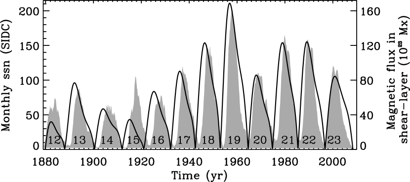
However, the predictive skill has been limited to hindcasting the peak-amplitude of a cycle in those calculations; for example, see Figure 1. Here a simulated sequence of cycles derived from a tachocline toroidal flux integral has been superimposed on observed cycles of monthly smoothed sunspot number (taken from www.sidc.be). The details within a cycle, such as its shape and its rise and fall patterns, have not been reproduced. In order to be able to predict the amplitude, timing and shape of a cycle simultaneously, we need to go beyond simple data-nudging for the entire span of integration. Updating the unknown time variations in the dynamo ingredients in a finite interval within a cycle, say every six to twelve months, will be required. Therefore, we need to implement a sophisticated data-assimilation scheme.

Figure 1: Gray-filled curve shows observed cycles derived from monthly smoothed sunspot number data from the Royal Observatory of Belgium (www.sidc.be); superimposed on that is a simulated sequence of cycles (black curve) derived from total tachocline toroidal flux integral. Simple data-nudging for 12 successive cycles can hindcast the cycle-peaks with high skill, but not the details within a cycle.

Modern Earth system prediction models use sophisticated data assimilation methods to capture all the usable observational information about the system. These methods are highly developed for atmospheric and oceanic predictions (Kalnay, 2003), but have only recently begun to be used for the Sun (Brun, 2007; Kitiashvili & Kosovichev, 2009; Jouve, Brun & Talagrand, 2011). With our present motivation of simulating cycle-shape and its rise and fall patterns, a suitable method is the Ensemble Kalman Filter (EnKF) technique in the framework of Data Assimilation Research Testbed (DART), which has been widely developed at the National Center for Atmospheric Research (Anderson, 2001; Anderson et al, 2005; Anderson & Collins, 2007; Anderson, 2009). Identifying the parameters which govern the spatio-temporal pattern of meridional flow as the so-called state vectors, we can apply an Ensemble Kalman Filter to these state vectors and can create an ensemble of time-varying magnetic fields by advancing our dynamo model. A built-in Monte Carlo step within DART selects the simulation closest to observation after each specified time advancement of the model within a solar cycle. If we advance the model sequentially over an entire solar cycle and determine the rise and fall patterns of that cycle that match best with observations, then we can construct the spatio-temporal pattern of meridional flow for an entire cycle. Similarly, if we know the spatio-temporal variations of meridional flow in a cycle, we can predict the shape, rise and fall patterns of that cycle.

Figure 2: Thick gray curve represents an observed cycle based on monthly smoothed sunspot number; superimposed on it is a corresponding simulated cycle measured by its tachocline flux integral. Successive dashed, dotted and dash-triple-dotted curves describe a sequential data-assimilation method with three successive flow variations during the forward time-advancement of the dynamo model. Meridional flow-speed is adjusted in the model after each specified time-interval during a simulation-run. Combining the curves – dashed, dotted and dash-triple-dotted curves and those beyond – one member of the Ensemble can be constructed.

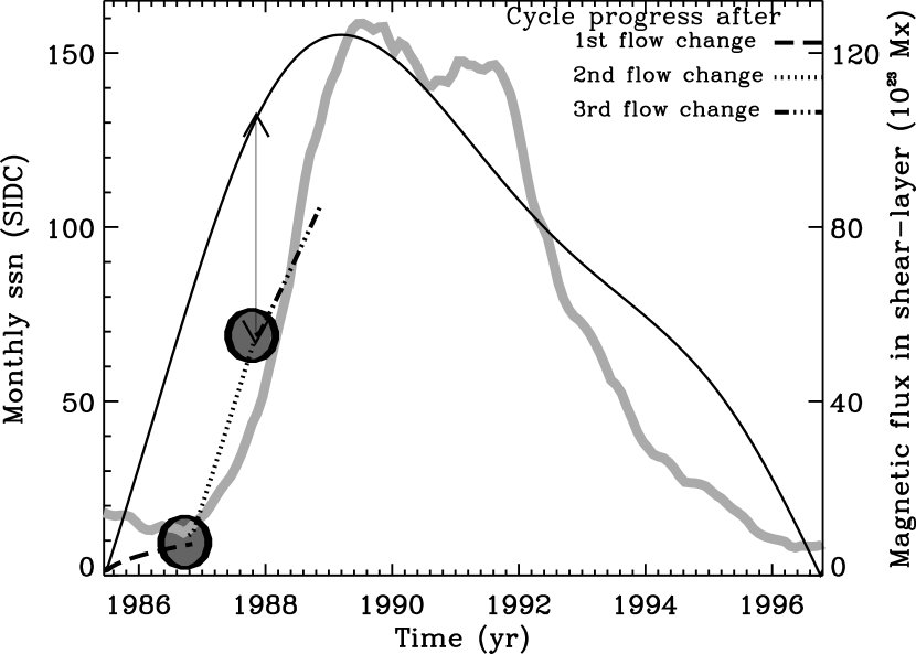
Figure 2 describes how the cycle shape can change when the meridional flow speed changes after a specified time. From Figure 1, the observed cycle 22, derived from monthly smoothed sunspot number data, has been plotted in Figure 2 as a thick gray curve, and the simulated cycle (black curve) has been superimposed on it. As an example, Figure 2 clearly reveals that the simulated cycle’s rise and fall patterns do not match with that of the observed one, because the simulation was performed with a steady meridional flow (see Dikpati & Gilman (2006) for details). Spatio-temporal variations in meridional flow were not known before the 1980’s. Very recently the surface flow-patterns as functions of latitude and time are being detected (Ulrich, 2010) (see also Guerrero, Rheinhardt, Brandenburg, & Dikpati (2011)). So, running the dynamo simulation, including updating the meridional flow speed after a specified time, and checking how the model-output compares with the observation, we can construct members of the Ensemble for a desired solar cycle (e.g. cycle 22, the example in Figure 2) and also the spatio-temporal variations of the meridional flow for that cycle.

From our prior knowledge of the properties of flux-transport dynamos, we can make certain guesses about how the simulated cycle’s phase will progress as the meridional flow varies. For example, near the beginning of the cycle (see Figure 2), we see that the simulated cycle-phase has progressed much faster than the observed one. Among various possibilities, a decrease in the flow-speed would make the cycle-phase progress more slowly, as shown by the dashed line. After a specified time, by comparing model-output with observations, the flow-speed can be updated again, with the aim of securing the closest possible match of the model cycle phase with the observed phase.

In this regard, it is first necessary to know which ingredients in the model determine the shape of a cycle, how those ingredients vary with time and how the model responds to their time-variation. Previous flux-transport dynamo studies (Dikpati & Charbonneau, 1999) indicate that the meridional circulation is the key ingredient that determines the timing and shape of a cycle. We know from observations that the meridional circulations vary substantially with time for both the Earth and the Sun. Perturbations in meridional flow are likely to be particularly important, since from considerations of mass conservation these perturbations are likely to be felt rather quickly throughout the model domain.

However, to make effective use of all the observational data available to predict future behavior of the Sun or Earth system, it is important to determine the ’response time’ of these systems to perturbations of various types and durations occurring at various places within the system. This has been studied extensively for ocean circulation and climate systems (Neelin, 2011; Andrews & Allen, 2008; Stouffer, 2004; Stouffer, Russell & Spelman, 2006; Stouffer & Manabe, 1999; Hoffert, Callegari & Hsieh, 1980; Battisti & Hirst, 1989), but not yet for the solar case. There does not appear to be a single ’response time’, but rather a continuous range of times, beginning soon after the time the meridional circulation starts changing, continuing through a time of ’peak’ response, followed thereafter by a time of declining further response. The time of peak response itself varies considerably, depending on the duration and location of the perturbation introduced, as well as the range of timescales inherent in the physics of the model. The model may respond quite differently to a perturbation of long duration compared to one of very short duration (for a discussion of this point in the case of climate systems, see Neelin (2011) section 6.8).

Comparison of the solar cycle prediction problem to that for the prediction of the Earth’s climate system is particularly instructive. It is well known (Neelin, 2011) that Earth’s climate and its variations in time are determined by interactions among the various major components of the Earth ’system’ (atmosphere, oceans, land surface, polar ice caps) as well as by external solar forcing. These interactions and forcings occur on a wide range of timescales, from days to centuries and millennia (Jöckel, Brenninkmeijer & Lawrence, 2000; Dickey, Marcus & Chin, 2007; White, Dettinger & Cayan, 2000; Foukal, Fröhlich, Spruit & Wigley, 2006; Jones, Ito, & Lovenduski, 2011; Chan & Motoi, 2005). This is analogous to, but even more complex than, the Sun’s ’climate’ system, or the solar dynamo, in which timescales of days (for emergence of new magnetic flux in active regions) to years (for variations in the Sun’s ’conveyor belt’ or meridional circulation) to a decade or two (for transport of magnetic flux to the bottom of the convection zone) and beyond (for the envelope of the solar cycle and the occurrence of ’Maunder minima”) are prominent.

In the Earth system, with the exception of the surface mixing layer, the timescales in the ocean are much longer than those in the atmosphere. They range from months to years for the layer above the thermocline, to decades to millennia for the deeper ocean. It follows that to predict changes in climate on timescales longer than a few weeks, the dynamics and thermodynamics of the ocean must be included in the models that are used (Neelin, 2011; Cane, Zebiak & Dolan, 1986). Analogously, to simulate solar cycle properties requires models that capture the MHD of the whole solar convection zone, for which the timescales are much longer than for emergence of new magnetic flux at the photosphere. Mean field flux-transport dynamo models are among the simplest that do this.

In both the Earth and Sun meridional circulation plays a critical role in determining behavior of the respective systems on longer timescales (Wunsch, 2002; Gnanadesikan, Slater, Swathi & Vallis, 2005; Dikpati & Charbonneau, 1999; Dikpati, de Toma & Gilman, 2006; Dikpati & Gilman, 2006). The closely related ’signal storage’ capacity or memory in both systems is particularly important. In the ocean the memory of past temperature anomalies at the ocean-atmosphere interface is (Cane, Zebiak & Dolan, 1986) retained in the deeper ocean, brought there, and later back to the surface of the ocean, by meridional flow. Similarly, the memory of past photospheric magnetic flux patterns is retained deep in the convection zone, brought there by the predominantly inward meridional flow at high latitudes.

This memory provides the basis for prediction of changes in the climate of the Earth and Sun on timescales of years to a decade or two. For the Earth, these predictions are focused on El Nino and La Nina events, as well as associated extratropical changes (Cane, Zebiak & Dolan, 1986; Meehl et al, 2009). For the Sun, the focus is on predicting how certain global properties of solar cycles, such as peak amplitude, duration and shape differ from one cycle to the next. This paper begins the process of developing a more sophisticated data assimilation scheme by estimating a flux-transport dynamo model’s response time to variations in one of its crucial ingredients, the meridional flow. The results will be important for achieving skill in predicting details within a cycle, the cycle-shape, its rise and fall patterns.

2 Steps Towards Building Sequential Data Assimilation Procedure

In order to implement the EnKF sequential data assimilation scheme for the purpose of successfully predicting cycle-shape, we need essentially two steps: (i) develop the implementation procedure of the scheme in the case of a flux-transport dynamo model, (ii) determine precisely the response of that dynamo model to changes in ingredients that govern the cycle-shape. In this particular class of dynamo models, the spatio-temporal variations in meridional flow are the most important ingredients for creating the variation in the progress of a cycle’s phase (Dikpati, Gilman, deToma & Ulrich, 2010), and hence the shape of that cycle. Therefore we wish to build a data assimilation scheme for our dynamo model that makes use of available data on variations in meridional flow on the Sun. In order to do an ensemble of simulations that optimizes use of the information contained in the meridional flow data, we must first determine the ’response time’ of the dynamo model to changes in meridional flow. This will give us essential guidance about, for example, what time interval over which to integrate the dynamo equations before adjusting the flow. Each segment of the model-run using sequential data assimilation should be long enough to allow the physical system to feel the change, but not so long as to degrade the time resolution of the simulated amplitude compared to the observed one. We explain how we do the response time calculation in section 2.3. The results of these calculations are shown in section 3.

2.1 Dynamo equations

The dynamo equations we use here are the standard ones for flux-transport dynamos (Dikpati & Charbonneau, 1999), given by

$${\partial B\over\partial t}=-{1\over r}\left[{\partial\over\partial r}(r{u_{r}}{B})+{\partial\over\partial\theta}({u_{\theta}}{B})\right]+r\sin\theta({{\bf B}_{p}}.\nabla)\Omega\hskip 170.71652pt$$

$$\hskip 170.71652pt-{\bf{\hat{e}}}_{\phi}\thinspace.\thinspace\left[\nabla\eta\times\nabla\times{B}{\bf{\hat{e}}}_{\phi}\right]+\eta({\nabla}^{2}-{1\over r^{2}\sin^{2}\theta}){B},$$

$${\partial A\over\partial t}=-{1\over r\sin\theta}({\bf u}.\nabla)(r\sin\theta A)+\eta\left({\nabla}^{2}-{1\over r^{2}\sin^{2}\theta}\right)A+{S(r,\theta)B\over 1+{(B/B_{0})}^{2}}+{\alpha B\over 1+{(B/B_{0})}^{2}}.$$

in which, the notations have usual meaning: $A$ and $B$ are respectively the poloidal filed vector potential and toroidal fields, $u_{r}$ and $u_{\theta}$ are $r$ and $\theta$ components of meridional flow, $\Omega$ the differential rotation, $\eta$ the diffusivity, $S$ the surface poloidal source (works as a nonlocal $\alpha$-effect on toroidal fluxtubes risen to the surface from the tachocline) and $\alpha$ the tachocline $\alpha$-effect. $B_{0}$ is the quenching field strength, which may or may not be the same for the nonlocal and local poloidal field sources; however, in this calculation the value of $B_{0}$ is the same for both $\alpha$-effects.

2.2 Estimating Model’s Response Time to Flow-Change

Flux-transport dynamo simulations with steady flow revealed that the dynamo cycle period is inversely proportional to the flow-speed (Wang & Sheeley, 1991; Dikpati & Charbonneau, 1999). This result was obtained by changing the flow speed from a previously set speed and, assuming that it will remain steady for several cycles, the dynamo was relaxed for about 4 or 5 cycles to obtain a new, saturated solution. However, observations (Ulrich, 2010; Gizon, Birch & Sprüit, 2010) indicate that the flow speed varies within a cycle in a time shorter than 11 years. In that situation, the phase of the cycle should change accordingly, and in turn, determine the shape of that cycle.

In order to estimate the response time of the model to a variation in flow, we will be using a calculation of lag-correlation between flow change and cycle’s phase-change. Lag-correlation has been used in the calculation of response time of oceanic and atmospheric models to the variation of their ingredients (Yasunari, 1990; Barsugli & Battisti, 1998; Su, Neelin & Meyerson, 2005; Wu, Kirtman & Pegion, 2006). Correlation coefficients in general give a measure of linear association between two variables. Lagged correlations are obtained by correlating a lagged dataset (cycle’s phase change in our case) with another unlagged dataset (flow change) using the Pearson method. Lagged data are computed by shifting data by a certain unit of time, either forward or backward. In our case, we will choose the unit of time to be 15 days. This means we will shift forward the lagged data, the cycle’s phase-change, by multiples of 15 days with respect to flow-change data. We identify the forward lagged-time that exhibits the highest, positive correlation coefficient between the flow-change and cycle’s phase change with the time of peak response of our dynamo model to flow-change.

Although the lag-correlation methods have been widely used in the context of atmospheric and oceanic models’ response time calculations, it has not been used so widely in the solar models, and, to the best of our knowledge, never in the solar dynamo models. Hence a schematic diagram is presented in Figure 3 to describe the lag-correlation we will use in this paper. In all frames of Figure 3, $v_{0}$ denotes the amplitude of the steady flow, $v_{1}$, $v_{2}...v_{10}$, the amplitudes of the time-varying flow at different times $t_{1}$, $t_{2}....t_{10}$. In each frame of Figure 3, the first column denotes the times at which the flow has been changed, the second column the change in flow-speed with respect to the steady flow-speed, and the third column the phase difference between the two simulated cycles (the cycle with time-varying flow and that with steady flow). In order to obtain a lagged correlation with zero, $t_{1}$, $t_{2},....$ time-lag, the second column quantities are correlated with the third column quantities staggering in the way indicated by the arrows.

In order to carry out the lag correlation analysis in the present context, we must define the phase change of a cycle. It is known from previous studies that the increase (decrease) in meridional flow speed makes the cycle progress faster (slower). The change in cycle-phase caused by flow-variation should be reflected in a simulated cycle as, (i) an amplitude change at a specified time compared to the cycle-amplitude for a steady flow case at that time or, (ii) a change in cycle’s progress-time due to flow-variation to achieve a specified cycle-amplitude. Here we will use the first definition.

Figure 3: Frames a, b and c describe how lag correlations between flow-speed-changes (with respect to steady speed) and cycle-phase-changes (with respect to that with steady-flow case) are calculated. Frame (a) has no lag between flow-speed-changes and cycle-phase-changes, frame (b) has a $t_{1}$ lag (actually lead in our case here) and frame (c) has a $t_{2}$ time-lag (lead here) with respect to the initial time ($t_{0}=0$) when the flow-change starts.

Returning to Figure 2, we illustrate graphically what the phase change is according to definition (i). The solid, black curve in Figure 2 represents a simulated cycle with a steady meridional flow. Implementation of flow-change for a specified time would lead to change in the progress of the cycle, as shown schematically in dashed, dotted and dash-triple-dotted curves. At a specified time, the difference in cycle-amplitudes for steady and time-varying flow (respectively the solid, black curve and dotted curve) is shown by a two-sided arrow, which essentially represents the cycle phase-change as defined in (i). Note that the phase change is negative in this case.

Since we do not have observational guidance about variations in radial of meridional circulation with time, we will consider a fixed, single-cell meridional flow profile as used by Dikpati (2011), and vary the poleward surface flow-speed only. From mass conservation, this will cause instantaneously a proportional speed change everywhere, namely for the flow sinking near the pole, returning equatorward at the bottom of the convection zone and upwelling near the equator. Furthermore, we will use a sinusoidal variation in speed with time ($\sin(\pi\,t/2\,\Delta\tau)$) during a time-span ($\Delta\tau$) of 3 - 24 months within a cycle’s rising, peak or declining phase. This means the speed increases during the first half of the time-span and decreases during the rest, or vice versa. We will also perform a few experiments with more complex flow profiles. Moreover, due to lack of observational information about flow below the surface, we will consider meridional flow profile constrained by mass-conservation in the entire dynamo domain. Thus the flow will be a streamlined flow behaving in a self-similar fashion, namely the percentage change in the amplitude of the flow at a certain point at the surface will reflect the same percentage change at all points of the fluid.

Different forms of speed variation with time can be considered, but a step-function is not a good choice for studying response time of a model to any ingredient variation. For some very idealized physical systems, a step-function is sometimes used to represent the change in the physical parameters for which a system response is calculated. In all the work on response times in geophysical fluid systems cited above, only one, (Hoffert, Callegari & Hsieh, 1980) tried a step-function for the system to respond to (in their case involving deep ocean heat storage and its response to climatic forcing). They concluded that while some properties of response can be studied using a step-function, it is physically quite unrealistic, so they did not base their primary results on that form of change. Instead, as stated in Hoffert, Callegari & Hsieh (1980), they used smooth, quasi periodic variations, as many other investigations have done, because they are much closer to the underlying physics and what is observed. The same is true for the solar meridional circulation. We therefore take smoothly varying changes in meridional circulation, of durations suggested by reference to the observational analyses of Ulrich (2010), rather than sudden step-function like changes.

Simulated solar cycles can be constructed in many ways. The cyclic variation of tachocline toroidal magnetic field at a selected latitude can be extracted (see Charbonneau & Dikpati (2000)), because that is the spot-producing field. Dikpati & Gilman (2006) used a tachocline toroidal flux integral within sunspot latitudes (equator to $45^{\circ}$) to construct theoretical solar cycle for comparing with observed spot-area cycle. Here we will use three different measures for the simulated cycles: (i) tachocline toroidal field ($B_{\phi}$) at $15^{\circ}$ latitude, (ii) $B_{\phi}$ at $60^{\circ}$, (iii) total tachocline toroidal flux integrated from the equator to pole.

3 Results

We calculate the time of peak response of a flux-transport dynamo model for which all the settings of the dynamo-ingredients, the differential rotation, meridional circulation, surface and bottom $\alpha$-effects, magnetic diffusivity and $\alpha$-quenching, are as used in Dikpati, Gilman, deToma & Ulrich (2010) (see also Dikpati (2011) for dimensional and non-dimensional parameter values for meridional circulation). We solve the dynamo equations in the northern hemisphere using a single-cell meridional flow profile.

3.1 Model’s response to flow variation with 9 months’ duration

As mentioned in §2.3, we consider a sinusoidal variation in meridional flow speed with a maximum amplitude of 50% of the steady flow. We first present the results in Figures 4-7, for the flow variation that lasts for 9 months ($\Delta\tau=9$ months). These figures respectively show the results for three distinct cycle-proxies for simulations of the same sequence of cycles: tachocline toroidal field $B_{\phi}$ at $15^{\circ}$ (Figures 4 and 5), $B_{\phi}$ at $60^{\circ}$ (Figure 6) and the total tachocline toroidal flux integral (Figure 7).

Figure 4: Top and middle frames in left column show respectively variation in meridional flow-speed for 9 months during the rising phase of a cycle (frame a) and cyclic toroidal magnetic field at $15^{\circ}$ latitude for steady (black) and time-varying flows (blue and red) (frame b). Bottom frame (c) shows how change in cycle-phase correlates with change in flow-speed as function of time (blue-diamonds are for flow increase with respect to steady flow and red-filled circles are for flow decrease). The time at which cycle-phase-change has the highest correlation with flow-speed-change is a measure of the model’s time of peak response to flow variation. Frames d, e, f show the same information as in frames a,b,c respectively, for variation in flow speed during the declining phase of the cycle.

Figure 5: Enlargement of first 1.5 years of response of tachocline toroidal field at $15^{\circ}$, for the case shown in Figure 4.

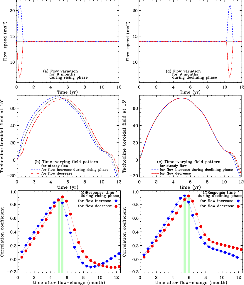
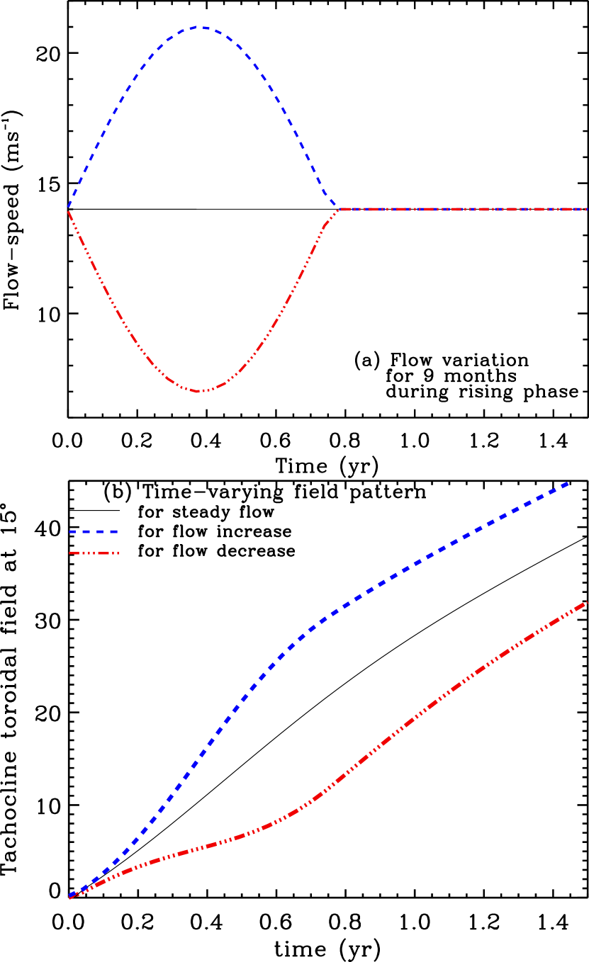
$B_{\phi}|_{{\rm at}15^{\circ}}$ should be a good proxy of the sunspot cycle because $15^{\circ}$ is approximately the peak sunspot latitude. This proxy has been used in the past in flux-transport dynamo simulations (see, for example, Charbonneau & Dikpati (2000)). The three frames in the left column of Figure 4 show the result for flow variation that occurs during the rising phase of the cycle (Figure 4a), in the form of an increase (blue curve) or decrease (red curve) with respect to the steady flow (black curve). In Figure 4b we display the profiles of toroidal field $B_{\phi}$ as functions of time; black curve denotes the cycle with steady flow and blue and red curves represent that with time-varying flow as shown in Figure 4a. The bottom frame (Figure 4c) shows the lag-correlation coefficients, plotted in blue diamonds for flow increase and in red circles for flow decrease. The right column (Figures 4d-f) shows the analogous plot when the flow change occurs during the declining phase of the cycle.

The results seen in Figures 4 and 6 are in many ways quite similar, implying that they do not depend significantly on the choice of latitude for the proxy toroidal field. In both cases, for meridional flow perturbations in both ascending and descending phases, the cycle advances in phase faster when the meridional flow is increased temporarily, and slower when it is decreased (Figures 4b,e; 6b,e). This effect is to be expected, given that in flux-transport dynamos, the cycle period is largely determined by the meridional flow speed (Dikpati & Charbonneau, 1999).

The lag-correlation coefficients in Figures 4c, 4f, 6c, 6f all start with a low value at the beginning of flow-variation, slowly increase with the increase in time-lag between the cycle-phase and flow-change, reach a peak and then decline rapidly. From the lag time of the occurrence of the peak, we estimate the time of peak response of the model to the flow change to be 5 to 6 months for both proxies. But from Figure 5 we can see that the model slowly starts responding to the change in meridional flow within one month after the meridional circulation starts to change. So we are measuring the time of peak response; the system starts to respond almost immediately.

Figures 4 and 6 reveal that the peak in lag-correlation coefficient for the case with flow-increase (blue diamonds) always occurs a few months before that with flow-decrease (red circles). This means that the model responds a little faster to an increase than a decrease in flow speed. We speculate that this difference occurs because when the speed is increased at every point in the domain, the ’signal’ of change is transmitted faster to neighboring points, making it possible for the whole system to adjust faster to the change. The opposite occurs when the flow is decreased everywhere.

Figure 6: Same as in Figure 4, but for the tachocline toroidal field at $60^{\circ}$.

Figure 7: Three frames in left column present changes in cycle pattern for total tachocline toroidal flux, due to changes in flow during rising phase (frame a), declining phase (frame b) and cycle-maximum phase (frame c). Frames (d-f) in right column present the corresponding lag-correlation coefficients.

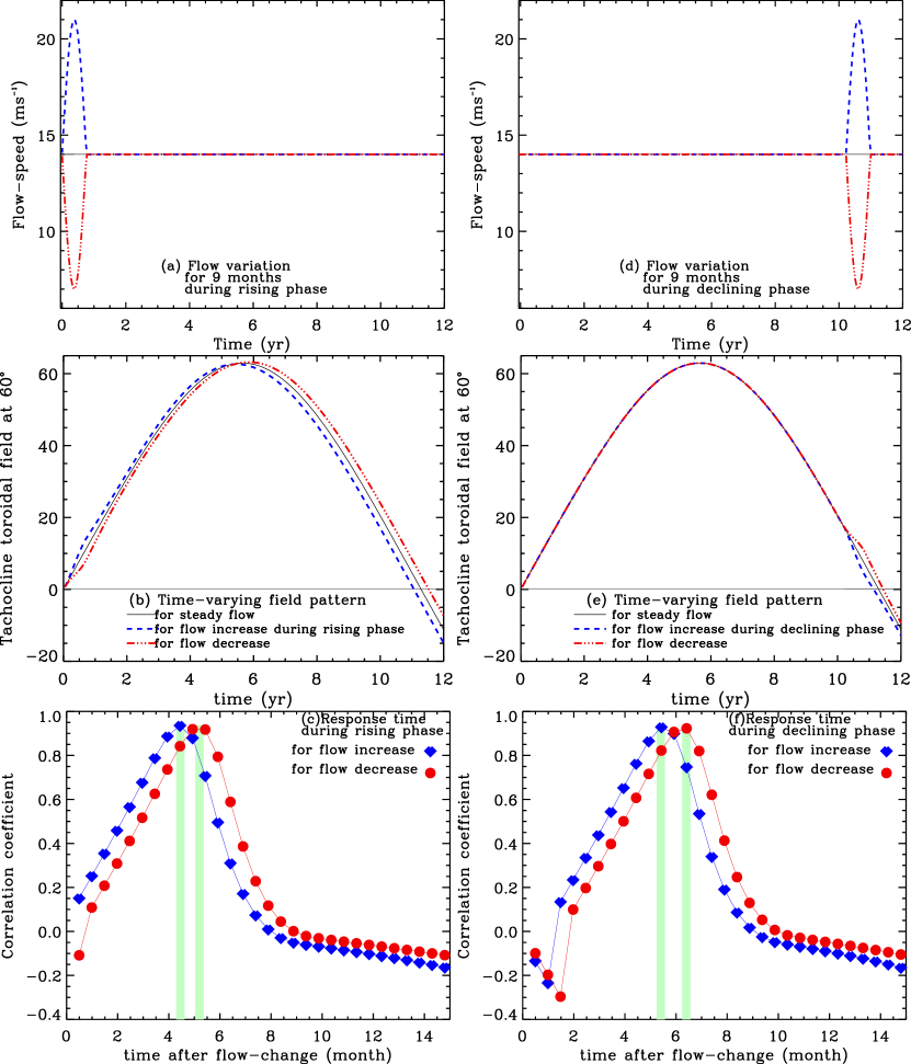
Comparing Figures 4c with 4f and 6c with 6f, we find that the model’s time of peak response to the flow-change is slightly longer (by about a month) in the declining phase than in the rising phase. It is less clear what causes this difference, but it may have to do with the fact that during the rising phase, toroidal fields are being amplified without change of sign, while in the late declining phase the toroidal fields are declining and going through a sign change.

The correlation also has a substantial time duration (a few months), rather than a spike, indicating that the model responds over a range of time-scales, whose peak is about 5 months in this case. This is what we should expect in a system in which advection by meridional circulation and diffusion are competing with each other; in other words the magnetic fields are only partially frozen in the plasma, unlike an ideal MHD case where we may find a delta function type response of the model.

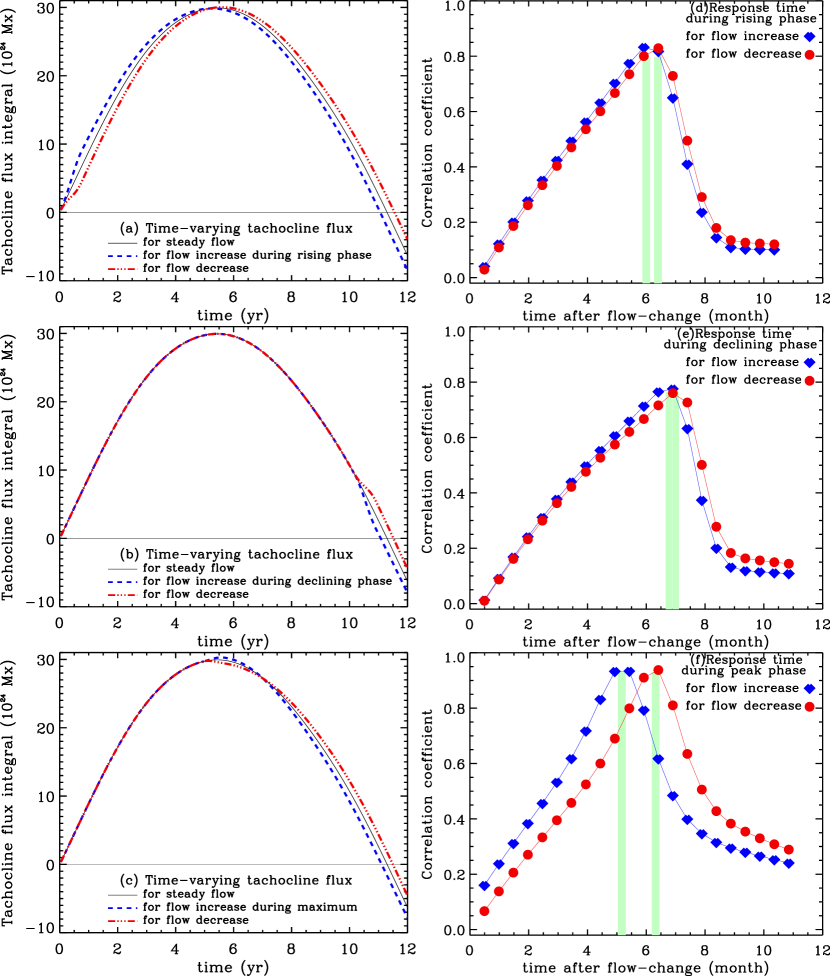
Figure 7 shows the profiles of lag-correlations for the total tachocline flux integral for meridional flow perturbations of nine month’s duration for three cycle phases: ascending and declining phases as seen in Figures 4 and 6, and also near peak phase. We see that for this proxy of the cycle, the time of peak response during the declining phase is close to a month longer than during the rising phase, similar to what was found from toroidal fields at $15^{\circ}$ and $60^{\circ}$ seen in Figures 4 and 6. On the other hand, the difference in response time for flow increases and decreases has shrunk. This is probably because the effect of a given change in meridional flow is different at different latitudes, and all latitudes of the tachocline are included in the flux integral. By contrast, Figure 7f shows that near cycle maximum the difference in response time between flow increase and decrease is even larger. From Figure 7c, it seems clear that near maximum, speed-up or slow-down in phase advancement becomes convolved with changes in peak amplitude. The higher peak from flow increase comes later than the lower peak with flow decrease, but this apparent phase difference is reversed as the declining phase progresses.

3.2 Model’s response to variation in the meridional flow-speed durations shorter and longer than 9 months

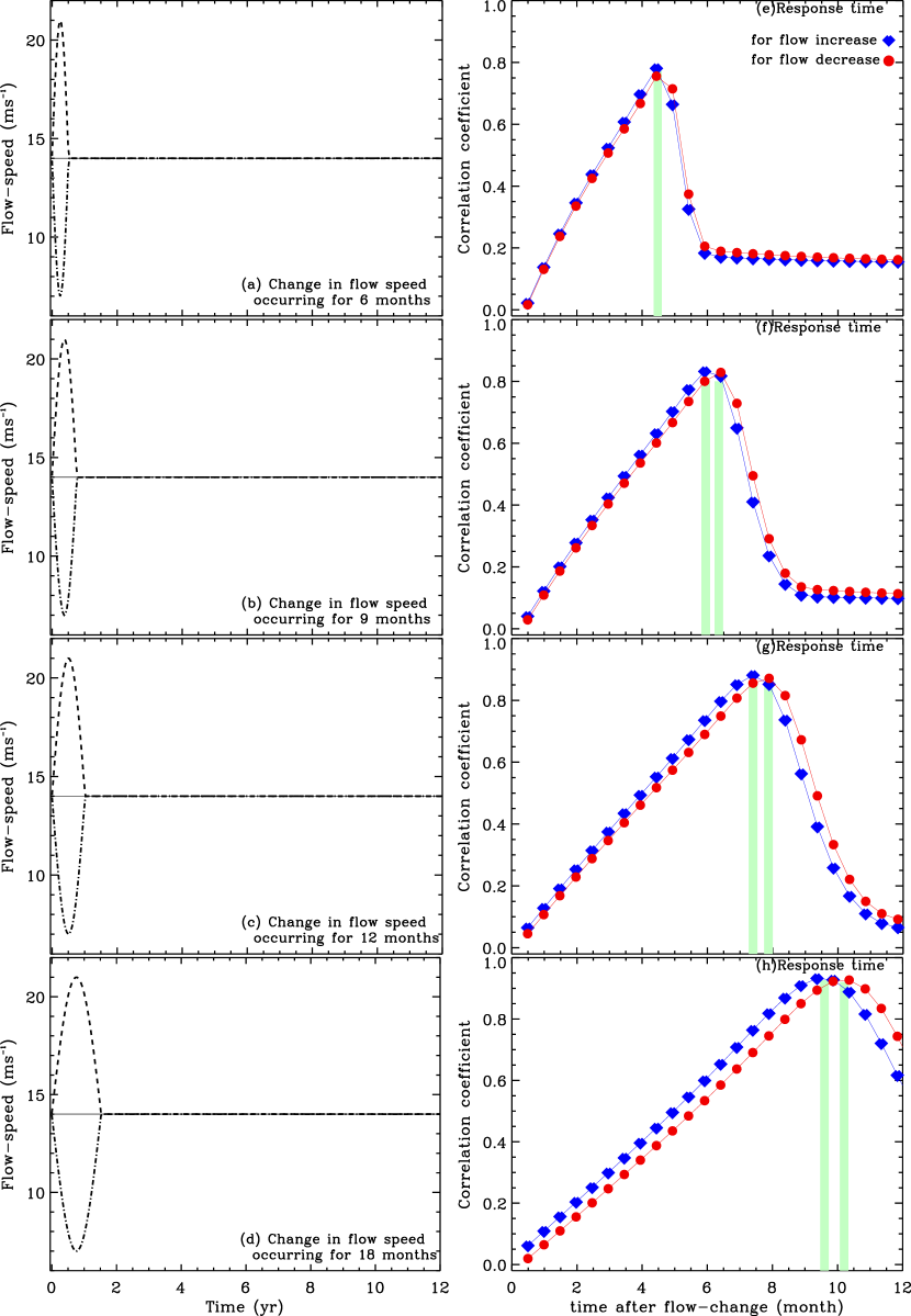
For results presented so far, we have chosen a meridional circulation perturbation that lasts nine months. What happens when the length of this perturbation is changed? Figure 8 gives the answer. Here we display the lag correlations for meridional circulation perturbations of the same profile but durations of 3,4,6,9,12 and 18 months. As the duration of perturbation is lengthened from 3 to 18 months, several features are revealed. First, the time of peak response increases, approximately in proportion to the duration of the perturbation. To first order, the time of peak response remains close to the time width of the meridional flow perturbation at the point of full width at half maximum. But by 24 months, the response time is somewhat shorter than that value (10 months vs 12 months). We judge this to be a real effect, because the response time should remain finite in the face of a permanent change of the meridional flow speed. There should be an asymptotic response time in the system as the duration of the meridional flow perturbation is increased. We have not attempted to find this asymptotic value, but it is clearly longer than ten months in the flux-transport dynamo we have used.

Second, the difference between the time of peak response for flow increase and flow decrease also increases; the systematic increase in the separation between the two vertical pale green marks from top right frame towards the bottom right frame of Figure 8 is clearly evident. As seen earlier in Figures 4, 5, 6 and 7, the time of peak response is shorter in the case of flow-increase than in the case of flow-decrease. During the forward progress of the cycle the increase in flow helps the cycle progress faster and hence, the increase in flow helps transmit the change faster to neighboring points of the domain than that in the case of flow decrease. The more enhanced is this effect, the longer is the duration of flow perturbation.

We compare the times of peak flow-perturbation and peak response for a wide range of perturbation durations in Figure 9. The left hand scale gives both peak times in months, while the right hand scale is a measure of the difference between these times, normalized by the duration of the flow perturbation (twice the time to the peak of the flow- perturbation). We see that for long peak times, their normalized difference approaches zero, i.e., the model responds at about the same rate as the applied perturbation. But for short durations, the normalized difference reaches 0.5, meaning the time of peak response is twice as long as the time to peak perturbation. It appears this ratio will get even larger for perturbations of even shorter duration; this is pushing the limit of applicability of a mean-field formulation. Nevertheless, by extrapolation of the plots of peaks to zero duration, it appears that the shortest possible peak response time is about 1.5 months. But as we have shown, for a more typical meridional flow perturbation of 3-18 months, the response is spread over a much longer time period.

Figure 8: Four frames from top to the bottom in left column present flow-changes with different durations, respectively for 6, 9, 12 and 18 months. Corresponding lag-correlation coefficients between total tachocline toroidal flux and flow-variation have been plotted in frames (e-h) in right column.

Figure 9: Comparison of times of peak flow perturbation and peak response

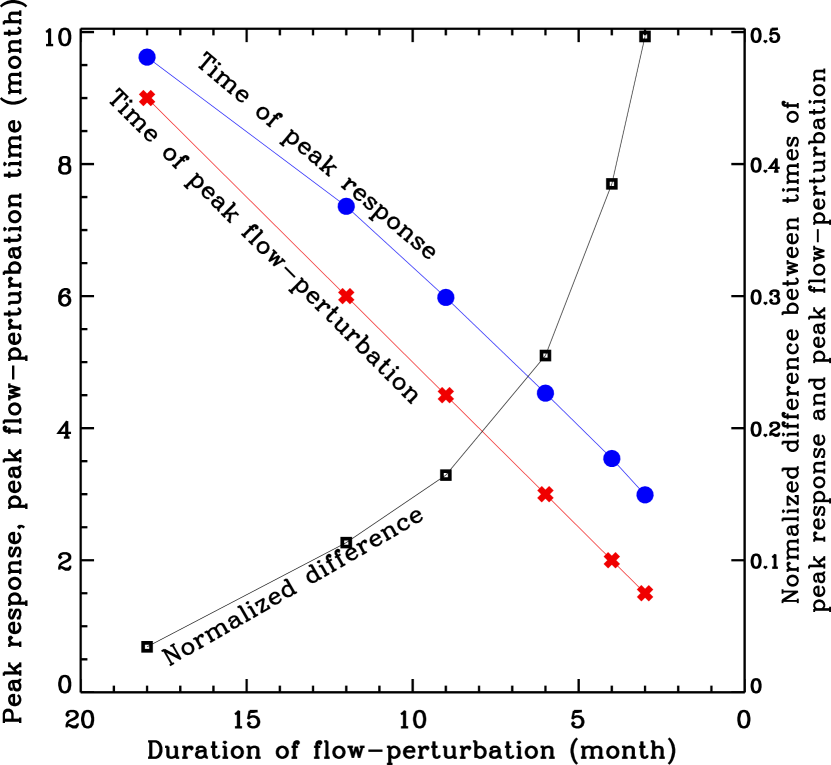
The shortest possible peak response time should be greater than zero, because it takes a certain time for the effect of the changed meridional circulation amplitude to be transmitted from grid point to the next. Since our calculations are for an advection-dominated dynamo, advection times will be shorter than diffusion times, but all ill contribute. We used 101 grid points between inner and outer boundaries, and the same between equator and pole. Therefore, the transmission time is four times longer between adjacent points in latitude than between adjacent radial points, for the same velocity. But mass continuity, the latitudinal flow is $\sim 4$ or 5 times larger than the radial flow; therefore the advection times between adjacent grid points are roughly the same in radial and latitudinal directions. For example, for an average latitudinal flow speed of $4\,{\rm m}{\rm s}^{-1}$ and radial speed of $1\,{\rm m}{\rm s}^{-1}$, the transmission time is about 23 days. We should expect the peak response to be reached in a somewhat longer time than 23 days; we found it roughly to be 1.5 months in the present calculations.

3.3 Model’s response to variation in the meridional flow-speed in the case of a higher diffusivity

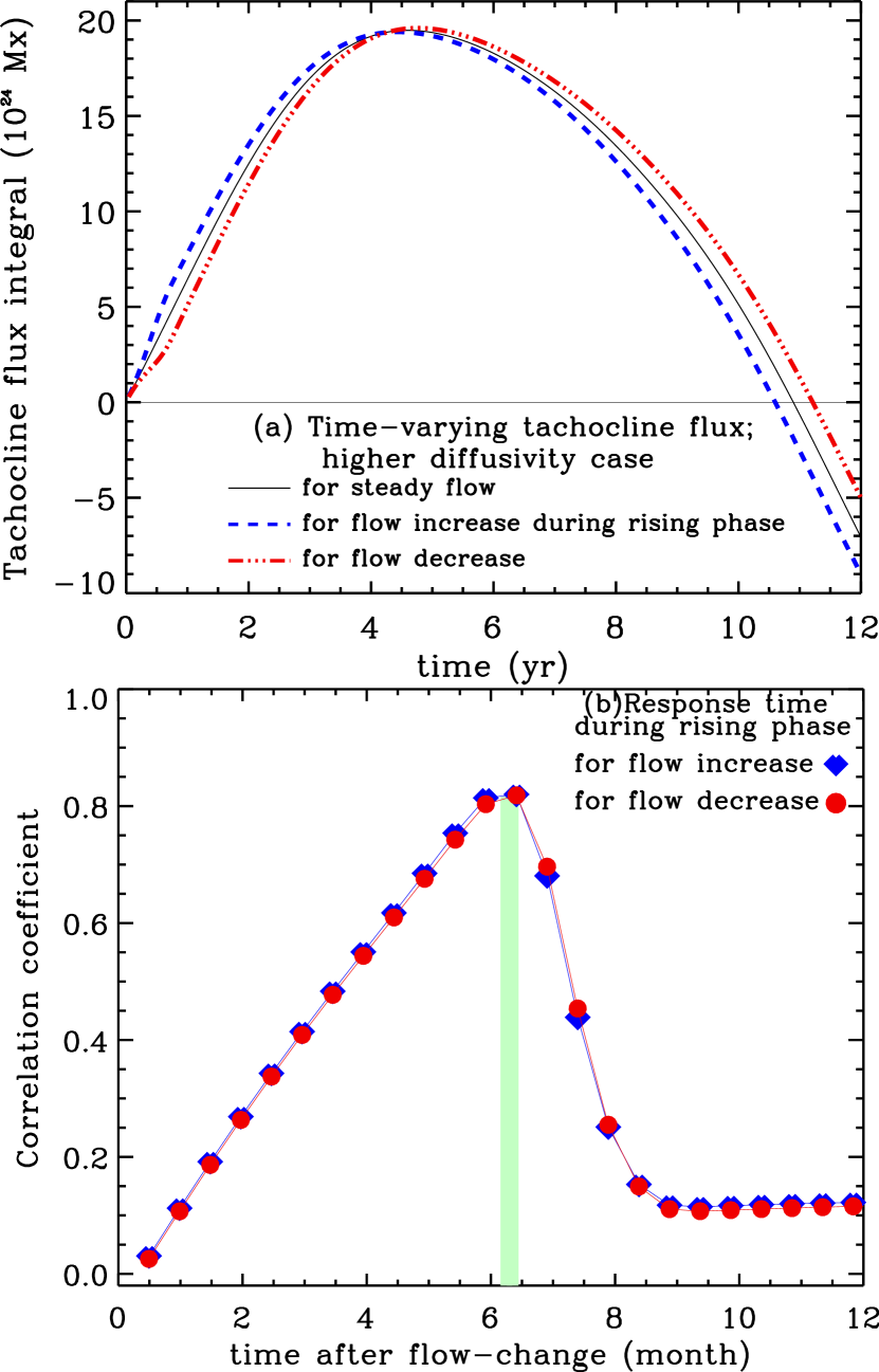
Another physical parameter that the time of peak response could be sensitive to is the magnetic diffusivity. Figure 10 displays the time variation in toroidal flux integral and the lag correlation for a meridional flow perturbation for nine months, applied during the rising phase of a dynamo solution with the magnetic diffusivity of the bulk of the dynamo domain doubled to $10^{11}\,{\rm cm}^{2}\,{\rm s}^{-1}$. We see that the time of peak response remains about six months, essentially the same as found for the lower magnetic diffusivity case shown in Figure 7d. We infer from this result that as long as the dynamo is operating in the advection-dominated regime, the response time does not depend significantly on the diffusivity. For the dynamo model we have used, solutions with magnetic diffusivity smaller than about $2\times 10^{11}\,{\rm cm}^{2}\,{\rm s}^{-1}$ are advection dominated. For substantially higher diffusivities, when diffusion dominates over advection, we would expect the time of peak response time to be influenced by the magnetic diffusivity value. We have not explored that regime here.

Figure 10: Toroidal flux integral and lag correlation profiles for a dynamo solution with double the magnetic diffusivity of solutions displayed in Figure 6. Meridional flow perturbation lasts 9 months and is applied during the rising phase of the cycle

3.4 Model’s response to a complex variation in the meridional flow-speed

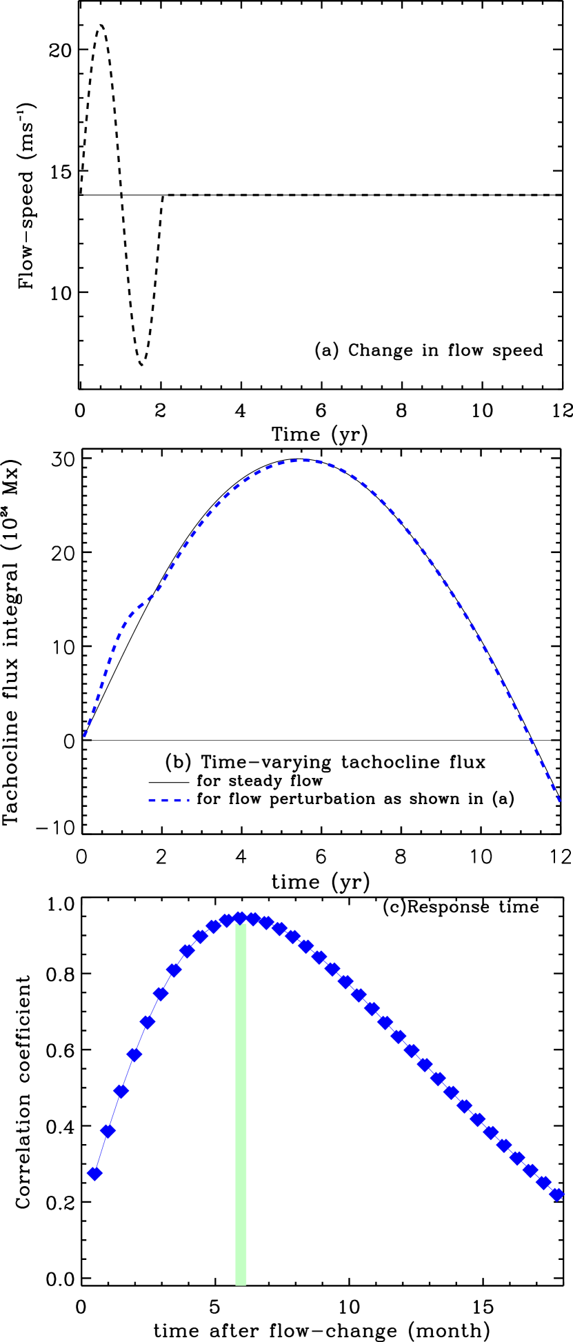
So far, we have done all of our numerical experiments performed with one particular profile of flow perturbation, namely a $\pm\sin(\Delta\tau)$ type profile for flow change with respect to the steady, mean flow. In this section, we perform two experiments to investigate how the model’s response time depends on the choice of flow perturbation profile and amplitude. In Figures 11(b) and (c), we present the time variation of toroidal flux integral and its lag correlation for a meridional flow perturbation as shown in Figure 11a. The duration of the flow perturbation is 24 months in this case; during the first 6 months the flow increases by 50%, and then continuously decreases during the next 12 months, so that the speed gets reduced by 50% with respect to the steady, mean flow of $14\,{\rm m}\,{\rm s}^{-1}$, and finally it increases again during the last 6 months of 24 months’ perturbation to reach the level of steady, mean flow speed.

The toroidal flux integral (TFI) in Figure 10b in the case of time-varying flow shows a fast phase advancement with respect to that for steady flow (thin black curve) and then a slow-down followed by a slight speed-up. The two TFI patterns (dashed blue and thin black curves) ultimately match in the late declining phase of the cycle. This is not surprising, because the time-averaged flow-speeds are the same in both cases (see Figure 11a). However, what is surprising is that the time of peak response in this case with more complex flow perturbation than that used in Figures 4-9 is again about 6 months (see Figure 11c), which is within a similar range of response times we found in §3.1, §3.2 and §3.3.

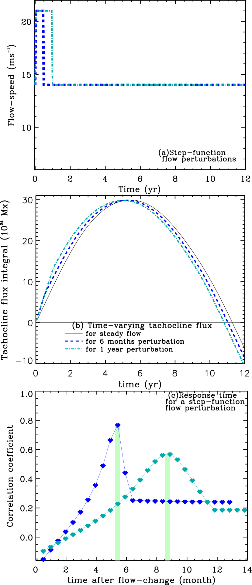
Although a flow perturbation in step-function form may not be a realistic flow variation in the case of solar meridional circulation, we show two cases to study the model’s response to flow variation in step-function profiles. Selecting two different durations of such flow variations, namely the perturbations lasting for 6 months and 1 year respectively (see blue-dashed and bluish green dash-dotted lines in Figure 12(a)) during the rising phase of a solar cycle, we compute the TFI and the model’s response to the above two flow perturbations and plot in Figures 12(b) and (c) respectively. Again blue-dash and bluish-green dash-dotted lines represent respectively the TFIs for flow perturbations with 6 months and 1 year duration. The response times of the model for these two cases of step-function flow perturbations are 5.4 months and 8.6 months respectively. This experiment gives another example of similar lag correlation and model’s response time as shown in Figures 4-9, indicating the robustness of a dynamo model’s response to meridional flow variation. The peak correlation is lower for a stepfunction of 12 months duration than for a sinusoidal perturbation of the same duration, because the flow perturbation peak itself is flat for a year, rather than strongly peaked.

Figure 11: Frames (a,b,c) respectively present flow variation, toroidal flux integral and lag correlation profiles for a dynamo solution with a different and more complex flow perturbation than that in Figure 4(a). Meridional flow perturbation lasts for two years and is applied during the rising phase of the cycle

Figure 12: Top frame presents step-function flow variation with durations of 6 months (blue-dashed line ) and 1 year (bluish-green dash-dotted line). Corresponding toroidal flux integrals and response times of the model are shown in frames (b) and (c) respectively.

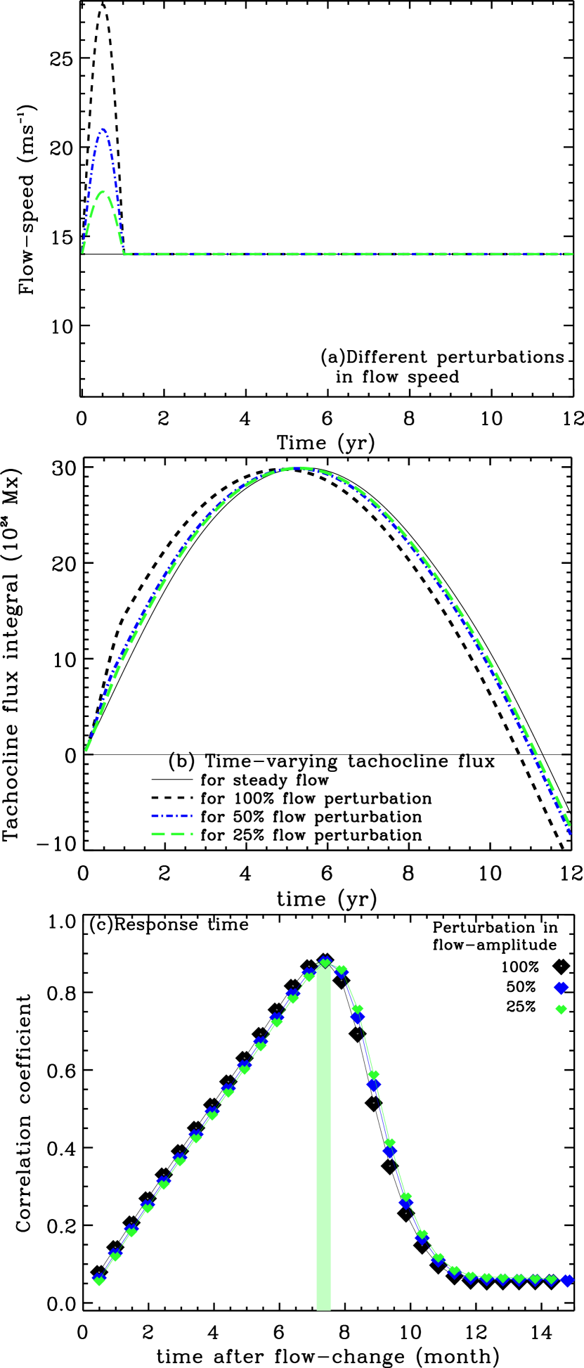
In order to investigate whether the amplitude of the flow perturbation can influence the model’s response to flow variation we perform dynamo simulations with different amplitudes of flow perturbation, namely 25%, 50% and 100% changes in flow speed with respect to the steady flow of $14\,{\rm m}\,{\rm s}^{-1}$. In the previous sections, we focused only on the model’s response to 50% change in flow speed. In Figures 13(a), (b) and (c), we respectively show the flow perturbation, the TFI and the response time. Flow perturbations with 25%, 50% and 100% amplitudes, compared to steady flow (thin black line in Figure 11a), are shown in green long-dashed, blue dash-dotted and black short-dashed lines. If we had included a case for which the flow amplitude was increased by 75%, this curve would have fallen in between the 50% and 100% curves. Corresponding TFIs in Figure 11b show that the changes in phase advancement are approximately proportional to the amplitudes of flow perturbations. Consequently lag correlation patterns, plotted in Figure 11c in small-sized green, medium-sized blue and large black diamonds respectively for 25%, 50% and 100% amplitudes of flow perturbations, almost overlap with one another. The time of peak response is 7.4 months, which indicates again that the model responds to the flow perturbation according to the inherent memory of the model (Yeates, Nandy & Mackay, 2008). The model’s time of peak response is not influenced by the amplitude of the flow perturbations because the the rate of cycle phase changes roughly in proportion to the rate of change of flow amplitude in this class of models.

Figure 13: Green dashed, blue dash-dotted and black long-dash lines in frame (a) present three different amplitudes of flow perturbations, 25%, 50% and 100% with respect to steady flow ($14\,{\rm m}\,{\rm s}^{-1}$). In frame (b) the corresponding curves present toroidal flux integrals and in frame (c) small-sized green, medium-sized blue and large black diamonds present lag correlation plots for the above three flow perturbations respectively. Flow perturbation lasts for 1 year and occurs during the rising phase of the cycle.

4 Discussion and Conclusions

Solar cycle prediction research has progressed significantly during recent years so that physics-based models are being integrated forward in time, in addition to using empirical relations. But so far those efforts have been limited to predictions of peak-amplitude of a cycle and its average duration. Attempts to predict simultaneously the shape, timing and amplitude of a cycle have not been made yet. With knowledge gained from advances in predictions employing oceanic and atmospheric climate models, it has proven necessary to move beyond simple data-nudging to more sophisticated data-assimilation techniques. Efforts using an Ensemble-Kalman Filter (EnKF) approach (Kitiashvili & Kosovichev, 2009) as well as variational approach (Jouve, Brun & Talagrand, 2011) have been made using one-dimensional dynamo models.

Prior results from flux-transport dynamo simulations reveal that the meridional circulation primarily governs the progress of a cycle’s phase in this particular class of dynamo models. The time variations in meridional circulation speed and profile can be used in a sequential data-assimilation approach that involves an EnKF method in the framework of the Data Assimilation Research Testbed (DART) (Anderson, 2009) in order to predict the details within a cycle, namely the rise and fall patterns, the onset, peak and end timings and the peak-amplitude.

A sequential data assimilation approach can be most efficiently used if we know the model’s response time to a change in its ingredients. Then we will know how to update the input data of a specific ingredient into the model. With this motivation we studied a flux-transport dynamo model’s response time to meridional flow-speed variations, and found that the model’s time of peak response to a change in flow-speed that lasts typically from one-half to one and a half years, is about six months on average. This response time is independent of proxies used to measure a theoretical solar cycle, such as tachocline toroidal field at $15^{\circ}$ latitude, at $60^{\circ}$ latitude or the integrated total toroidal flux in the tachocline. All response times are much shorter than the ’circulation time’ or the time it takes for a fluid element to make a complete circuit on a closed streamline that reaches both low and high latitudes as well as passing close to the inner and outer radial boundaries of the dynamo domain.

Incorporating changes in flow-speed lasting for different time-spans, such as 3, 6, 9, 12 and 18 months, we found that the time of peak response of the model increases with the duration of flow variation; it is approximately the length of full width at half maximum of the flow-perturbation profile in time. Response of the model is found to be always slightly faster when the flow change is positive with respect to the mean, steady flow, primarily because the rate of progress in a cycle’s phase is approximately proportional to the flow-speed in this class of dynamo models. We also found that the time of peak response is independent of magnetic diffusivity so long as the dynamo operates in the advection-dominated regime.

Although in most of our numerical experiments we chose a smooth sinusoidal type variation in flow-speed, we have also performed numerical experiments incorporating different shape and amplitudes of flow perturbations. We found that the model’s time of peak response to change in flow is roughly independent of the shape and amplitude of the flow perturbations.

There exists observations of systematic decrease of flow speed during the entire rising phase of the cycle 23 (Basu & Antia, 2003). Consideration of the flow speed change during such a long span of time for studying the response time of a dynamo models is beyond the scope of this paper. In a sequential assimilation scheme the unknown model ingredients require updating more frequently than on a solar cycle time scale in a dynamo model that is attempting to simulate shape of a solar cycle. So the experiments we have performed here have the perturbation lasting for no more than two years. However, it will be interesting to investigate whether a dynamo model would respond within the same cycle or in the next cycle to a systematic flow variation that occurs during an entire rising or declining phase.

We have focused only on the speed variation and taken no variation in latitudinal or radial flow profile, because we do not have information from observations about the complete flow-profiles in the convection zone. We can implement the knowledge gained here about the model’s response time to change in flow-speed to develop EnKF schemes for assimilating time-varying flow data sequentially and simulate a cycle’s rise and fall patterns along with its amplitude and timing.

Flux-transport dynamo models are particularly sensitive to a meridional flow changes; so its influence may be overestimated in this class of models. Data assimilation techniques are useful to better determine the relevant ingredients in the mean-field dynamo models and quantify their influence on observables like the magnetic cycle period.

References

- (1)
- Anderson (2001) Anderson, J. L. 2001, Mon. Wea. Rev., 129, 2884
- Anderson et al (2005) Anderson, J. L., Wyman, B., Zhang, S. & Hoar, T. 2005, J. Atmos. Sci., 62, 2925
- Anderson & Collins (2007) Anderson, J. & Collins, N. 2007, J. Atmos. and Oceanic Tech., 24, 1452.
- Anderson (2009) Anderson, J. L. 2009, IEEE Control Systems Magazine, 29, 66
- Andrews & Allen (2008) Andrews, D.G. & Allen, M.R. 2008, Atmos. Sci. Let., 9, 7
- Barsugli & Battisti (1998) Barsuglu, J. J. & Battisti, D. S. 1998, J. Atmos. Sci., 55, 477
- Basu & Antia (2003) Basu, S. & Antia, H. M. 2003, ApJ, 585, 553
- Battisti & Hirst (1989) Battisti, D.S. & Hirst, A.C. 1989, J. Atmos. Sci., 46, 1687
- Bélanger, Vincent & Charbonneau (2007) Belanger, E., Vincent, A. & Charbonneau, P. 2007, Solar Phys. 245, 141
- Brun (2007) Brun, S. 2006, Astron. Nachr., 328, 329
- Cane, Zebiak & Dolan (1986) Cane, M.A., Zebiak, S.E. & Dolan, S.C. 1986, Nature, 321, 827
- Chan & Motoi (2005) Chan, W. L. & Motoi, T. 2005, GRL, 32, L07601
- Charbonneau & Dikpati (2000) Charbonneau, P. & Dikpati, M. 2000, ApJ, 543, 1027
- Choudhuri, Chatterjee & Jiang (2007) Choudhuri, A. R., Chatterjee, P., & Jiang, J. 2007, Phys. Rev. Lett., 98, 131103
- Choudhuri, Schüssler & Dikpati (1995) Choudhuri A. R., Schüssler & Dikpati, M. 1995, A&A, 303, L29
- Dikpati (2005) Dikpati, M. 2005, Adv. Sp. Res., 35, 322
- Dikpati, Gilman & MacGregor (2005) Dikpati, M., Gilman, P.A. & MacGregor, K.B. 2005, ApJ, 631, 647
- Dikpati & Gilman (2007) Dikpati, M. & Gilman, P.A. 2007, Solar Phys., 241, 1
- Dikpati, Gilman, de Toma & Ghosh (2007) Dikpati, M., Gilman, P. A., deToma, G., Ghosh, S. 2007, Solar Phys. 245, 1
- Dikpati & Charbonneau (1999) Dikpati, M. & Charbonneau, P. 1999, ApJ, 518, 508
- Dikpati et al (2004) Dikpati, M., de Toma, G., Gilman, P.A., Arge, C. N. & White, O. R. 2004, ApJ, 601, 1136
- Dikpati, de Toma & Gilman (2006) Dikpati, M., de Toma, G. & Gilman, P.A. 2006, Geophys. Res. Lett., 33, L05102
- Dikpati & Gilman (2006) Dikpati, M., & Gilman, P.A. 2006, ApJ, 649, 498
- Dikpati (2008) Dikpati, M. 2007, Annales Geophysicae, 26, 259
- Dikpati, Gilman, deToma & Ulrich (2010) Dikpati, M., Gilman, P.A., deToma, G. & Ulrich, R.K. 2010, Geophys. Res. Lett., 37, L14107
- Dikpati (2011) Dikpati, M. 2011, ApJ, 733, 90
- Dickey, Marcus & Chin (2007) Dickey, J.O., Marcus, S.L. & Chin, T.M. 2007, GRL, 34, L17803
- Durney (1995) Durney, B.R. 1995, Solar Phys., 160, 213
- Foukal, Fröhlich, Spruit & Wigley (2006) Foukal, P., Fröhlich, C., Spruit, H. & Wigley, T.M.L. 2006, Nature, 443, 161
- Gizon, Birch & Sprüit (2010) Gizon, L., Birch, A. C. & Sprüit, H. C. 2010, ARAA, 48, 289
- Gnanadesikan, Slater, Swathi & Vallis (2005) Gnanadesikan, A., Slater, R.D., Swathi, P.S., & Vallis, G.K 2005, J. Climate, 18, 2604
- Guerrero, Dikpati, & de Gouveia Dal Pino (2009) Guerrero, G., Dikpati, M. & de Gouveia Dal Pino, E. 2009, ApJ, 701, 725
- Guerrero, Rheinhardt, Brandenburg, & Dikpati (2011) Guerrero, G., Rheinhardt, M., Brandenburg, A. & Dikpati, M. 2011, MNRAS, 375, L1-L5
- Hoffert, Callegari & Hsieh (1980) Hoffert, M.I., Callegari, A.J. & Hsieh, C.-T. 1980, JGR, 85, 6667
- Jöckel, Brenninkmeijer & Lawrence (2000) Jöckel, P., Brenninkmeijer, C.A.M. & Lawrence, M.G. 2000, JGR, 105, 6737
- Jones, Ito, & Lovenduski (2011) Jones, D.C., Ito, T. & Lovenduski, N.S. 2011, GRL, 38, L15604
- Jouve et al (2008) Jouve, L. et al 2008, A&A, 483, 949
- Jouve, Brun & Talagrand (2011) Jouve, L., Brun, A.S. & Talagrand, O. 2011, ApJ, 735, 31
- Kalnay (2003) Kalnay, E. 2003, Atmospheric Modeling, Data Assimilation and Predictability (Cambridge:Cambridge Univ. Press)
- Kitiashvili & Kosovichev (2009) Kitiashvili, I. & Kosovichev, A.G. 2009, Proc. GONG 2008/SoHO21, ”Solar-Stellar Dynamos as Revealed by Helio- and Asteroseismology”, p. 511
- Küker, Rüdiger & Schultz (2001) Küker, M., Rüdiger, G. & Schultz, M. 2001, A&A, 374, 301
- Li et al (2002) Li, K., Irie, M., Wang, J., Xiong, S., Yun, H., Liang, H., Zhan, L., Zhao, H. 2002, Publ. Astron. Soc. Japan, 54, 787
- Meehl et al (2009) Meehl, G.A. et al 2009, Bull. Am. Met. Soc., 90, 1467
- Merka, Merkova & Odstrcil (2007) Merka, J., Merkova, D. & Odstrcil, D. 2007, J. Atm. Solar-Terr. Phys., 69, 170
- Neelin (2011) Neelin, J.D. 2011, Climate Change and Climate Modeling (Cambridge: Cambridge Univ. Press)
- Ohl (1966) Ohl, A. I., 1966, Soln. Dannye. Byull., 9, 84
- Ohl & Ohl (1979) Ohl, A. I., & Ohl, G. I. 1979, NASA Marshall Space Flight Center Solar-Terrest. Pred. Proc., 2, 258
- Parker (1993) Parker, E.N. 1993, ApJ, 408,707
- Stix (1976) Stix, M. 1976, A&A, 47, 243
- Stouffer & Manabe (1999) Stouffer, R.J. & Manabe, S. 1999, J. Climate, 12, 2224
- Stouffer (2004) Stouffer, R.J. 2004, J. Climate, 17, 209
- Stouffer, Russell & Spelman (2006) Stouffer, R.J., Russell, J. & Spelman, M.J. 2006, GRL, 33, L17704
- Su, Neelin & Meyerson (2005) Su, H., Neelin, J. D. & Meyerson, J. E. 2005, J. Climate, 18, 4195
- Ulrich (2010) Ulrich, R.K. 2010, ApJ, 725, 658
- Ulrich & Boyden (2005) Ulrich, R.K. & Boyden, J.E. 2005, ApJ, 620, L123
- Yasunari (1990) Yasunari, T. 1990, Meteorol. Atmos. Phys., 44, 29
- Yeates, Nandy & Mackay (2008) Yeates, A. R., Nandy, D. & Mackay, D. H. 2008, ApJ, 673, 544
- Wang & Sheeley (1991) Wang, Y. M. & Sheeley, N.R.,Jr. 1991, ApJ, 383, 431
- White, Dettinger & Cayan (2000) White, W.B., Dettinger, M.D. & Cayan, D.R. 2000, Proc. 1st Solar & Space Weather Conf., ’The Solar Cycle and Terrestrial Climate’ (ESA SP-463), 125
- Wu, Kirtman & Pegion (2006) Wu, R., Kirtman, B. P. & Pegion, K. 2006, J. Climate, 19, 4914
- Wunsch (2002) Wunsch, C. 2002, Science, 298, 1179