The origin of order in random matrices with symmetries
Abstract
From Noether’s theorem we know symmetries lead to conservation laws. What is left to nature is the ordering of conserved quantities; for example, the quantum numbers of the ground state. In physical systems the ground state is generally associated with ‘low’ quantum numbers and symmetric, low-dimensional irreps, but there is no a priori reason to expect this. By constructing random matrices with nontrivial point-group symmetries, I find the ground state is always dominated by extremal low-dimensional irreps. Going further, I suggest this explains the dominance of g.s. even for random two-body interactions.
One of the most ‘beautiful’ results in mathematical physics is Noether’s theorem. In classical mechanics a (continuous) symmetry leads to a conserved quantity, for example translational invariance leads to conservation of momentum, invariance under displacement in time leads to conservation of energy, and rotational invariance leads to conservation of angular momentum.
In quantum mechanics we can think about symmetries in terms of groups and their irreps. Group irreps divide up a Hilbert space into subspaces; if a Hamiltonian is invariant under a symmetry, meaning it commutes with the generators of a group, then the Hamiltonian becomes block-diagonal in the irreps.
For continuous symmetries, we label the irreps by quantum numbers, which in turn arise from the eigenvalues of the Casimir(s) of the symmetries. For discrete symmetries the Hamiltonian is still block-diagonal in the irreps, although lacking a Casimir there may not be a ‘natural’ quantum number labeling the irreps.
While Noether’s theorem is a powerful result, it tells us nothing about the relative ordering of states. In natural systems, however, we observe an ordering so striking and ubiquitous we tend to take it for granted, namely that the ground state and states lying low in the spectrum tend to belong to ‘small’ quantum numbers with the most symmetric wavefunctions. For example, under translational symmetry the ground state has momentum , under rotational symmetry the ground state has , etc.
Of course this arises because of physics: in most Hamiltonians the kinetic energy terms are quadratic in linear momentum and/or angular momentum . This in turn occurs because Nature, or physicists, prefer almost-local theories, and the first nontrivial non-local terms are quadratic in the gradient.
But surprisingly, even when one removes all trace of ‘physics’ the pattern remains. In nuclear structure this is seen in the discovery that many-body systems with rotationally invariant but otherwise random two-body Hamiltonians nonetheless tend to have ground states with , just like ‘realistic’ interactions, even though such states are a small fraction of the total spaceJBD98 ; ZV04 ; ZAY04 . This phenomenon is robust; for example while textbooks traditionally ascribe the g.s. to the pairing interaction BM ; simple , still dominates the ground state even when the pairing matrix elements are all set to zero Jo99 . It also occurs in boson systems BF00 such as the Interaction Boson ModelIBM . Over the past decade there have been many proposed ‘explanations.’ As the distribution of many-body systems with two-body interactions tend to have a Gaussian distribution of states MF75 , a number of authors have focused on widths BFP99 ; PW04 , while others have statistically averaged in a single -shell the coupling of multiple angular momenta MVZ00 . As a recent Letter stated, ‘the simple question of symmetry and chaos asks for a simple answer which is still missing Vo08 .’
To investigate this phenomenon, I propose a novel approach. In physics (as in art, that arbiter of ‘beauty’) we often delve deeper by stripping away assumptions to see what remains. Previous studies of random two-body interactions used shell-model diagonalization codes, but instead of carefully calculated matrix elements of two-body interactions they used random numbers, insisting only on rotational invariance. Now I go a step further: I abandon the shell-model framework, take random matrices, often used to investigate statistical properties of complex systems BM ; RM , and impose discrete rotational symmetries of the regular polyhedra upon them.
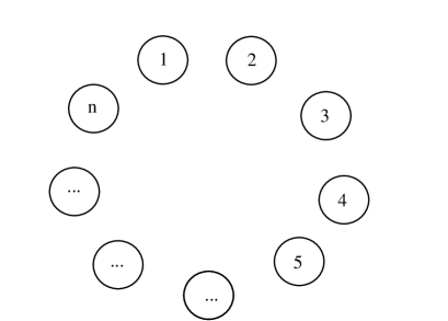
Let’s start with symmetry, the symmetry of discrete rotations in a plane. Figure 1 illustrates with loci evenly spaced in a circle. The generator of discrete rotations is
| (1) |
which send , and so on. One can easily show by hand that the most general real Hamiltonian invariant under discrete rotations is
| (2) |
where are random numbers. (Note: here and throughout I do not consider adding reflection symmetries, saving that for future work.)
One can solve this exactly without diagonalization by discrete Fourier transforms. One writes the matrix element in terms of a real function of a single index, so that, in (2), , etc.. The function from hermiticity, and by further inspection one gleans .
The next step is the Fourier decomposition of :
| (3) |
Inverting,
| (4) |
but using
| (5) |
where is the floor function and prevents double-counting when is even. It is easy to verify that . The are the eigenvalues of , and one is justified in using to label the different irreps. One can also find the eigenvectors easily; is the most symmetric, with constant, while is arguably the least symmetric, with .
While (5) gives the eigenvalues from a simple sum, we consequently have no a priori way of identifying the ground state energy which irrep it belongs to.
Next I assume there are additional degrees of freedom, as yet unspecified, and replace the scalars by real symmetric matrices so that
| (6) |
a matrix of dimension .
This matrix can no longer be immediately solved. What we can do, however, is to put into block-diagonal form, that is,
| (7) |
where
| (8) |
Here comes the key step. While we cannot analytically compute the ground state energy of each , we can compute the variance. If we assume the are independent random matrices, each with the same variance (assumptions which can be relaxed), then the variance of the th block is
| (9) |
For , this yields approximately , while otherwise this will yield approximately (because the average of ). Thus the matrices with will have the larger widths and the ground state will be one of those two.
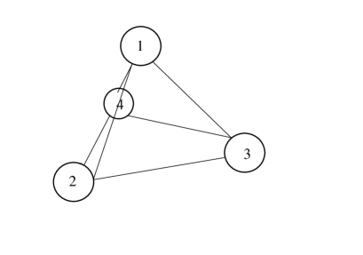
Now is an abelian group, but we can do the same analysis for other, nonabelian point-symmetry groups based on regular polyhedra. First, consider the tetrahedron, illustrated in Fig. 2. The most general Hamiltonian invariant under any discrete rotation about any of its facets is
| (10) |
Bringing this into block diagonal form,
| (11) |
That is, there is an irrep of dimension 1 with matrix and an irrep of dimension 3 with matrix . Again assuming are independent but have the same variance the variance of the 1-dimensional irrep (which has the most symmetric eigenvector) is while that of the 3-dimensional irrep is . All else being equal, the ground state is much more likely belong to the 1-dimensional irrep.
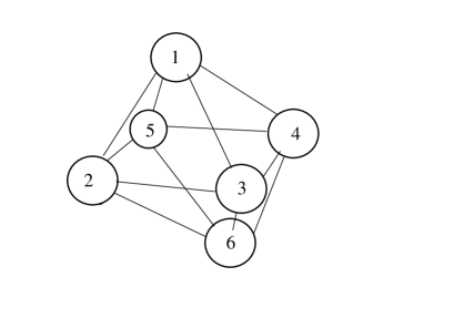
With the basic idea in hand, it is easy to consider other polyhedra. For the octahedron, Fig. 3, the invariant hamiltonian is
| (12) |
which has a 1-dimensional irrep, with matrix , a 2-dimensional irrep with matrix , and a 3-dimensional irrep with matrix . The variances are , , and , respectively.
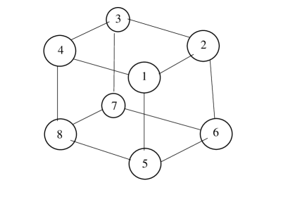
For the cube, Fig. 4, the Hamiltonian is of the form
| (13) |
with two 1-dimensional irreps with matrices and two 3-dimensional irreps with matrices . The 1-dimensional irreps have variance while the 3-dimensional irreps have variance .
While it remains to be proved in general, the lesson is clear: Starting with random matrices and imposing symmetries, the ground state is naturally dominated by certain irreps, generally irreps with lowest dimension.
Now I turn to continuous symmetries such as SU(2). I consider wavefunctions that can be written in the form where all of the rotational information is bound up in the spherical harmonic and refers to internal degrees of freedom SUV98 . I’ll return to the latter in a moment. Using the angles from spherical coordinates, the Hamiltonian is of the form , but imposing rotational invariance means can only depend on the angle between and as given by . Then where is a periodic function and, using Hermiticity (and assuming is real) is symmetric with respect to . Expanding
| (14) |
so clearly the are again the eigenvalues, with as eigenfunctions and with the eigenvalues independent of , as one expects.
Once more I assume to be a matrix-valued function, and thus to be a symmetric matrix given by
| (15) |
As before, let be the variance of the matrix elements independent of . Then I estimate the variance of the matrix elements of
| (16) |
Eqn. (16) can be computed numerically, and leaving off the factor , the values are 1.571, 0.393, 0.245, 0.178, 0.139 for respectively.
This suggests that in many-body system, subspaces with low-valued quantum numbers will have larger widths. But in realistic, finite many-body calculations, subspaces with different s have different dimensions. Furthermore, in the above argument each has independent random matrix elements, which typically has a semi-circular density of states RM , yet for many-body systems with only two-body interactions the density of states tends towards a GaussianMF75 .
I can approximately correct both deficiencies. First, following standard results on matrices with Gaussian-distributed matrix elements RM , I let be the width of the subspace of states with angular momentum . Then, for each , I simply create energies via a random Gaussian distribution of width , and ultimately determine the fraction of ground states with angular momentum .
Finally, I compare against a simulation via configuration-interaction calculations, that is, diagonalizing the Hamiltonian for fixed numbers of particles in finite single-particle spaces. Figure 5 shows the case of eight fermions (neutrons) in the --- shell-model space.
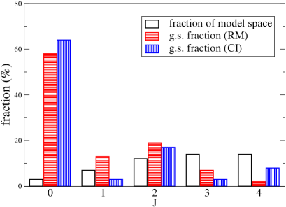
I take an ensemble of rotationally invariant, two-body but otherwise random interactions, and tabulate the fraction of states that have a given angular momentum . This should be compared with the native fraction of states with that in each many-body space, ( is the total dimension of the many-body space), and the fraction with is dramatically enhanced. I also compare with the fraction of ground states with a given predicted by my simple random matrix picture, . The only input are the dimensions and the universal variances computed in (16).
For such a simple picture, the random matrix model yields qualitatively excellent results, generally predicting the enhancement or suppression of different s in the CI simulations relative to the native fractions . The RM model successfully predicts an enormous enhancement of in the ground state, for this case and many others not shown due to lack of space.
This analysis suggests the predominance of angular-momentum zero ground states is primarily a function of the width of the angular-momentum-projected many-body Hamiltonian; furthermore, the width is largely decoupled from the microphysics, instead depending only on the projection integrand (16) and on the dimensionality of subspaces with good quantum numbers. The simplicity and decoupling from the microphysics may be why the phenomenon is so robust and so universal.
The U.S. Department of Energy supported this investigation through grant DE-FG02-96ER40985.
References
- (1) C. W. Johnson, G. F. Bertsch, and D. J. Dean Phys. Rev. Lett. 80, 2749 (1998).
- (2) V. Zelevinsky and A. Volya, Phys. Rep. 391, 311 (2004).
- (3) Y. M. Zhao, A. Arima, and N. Yoshinaga, Phys. Rep. 400, 1 (2004).
- (4) A. Bohr and B. R. Mottelson, Nuclear Structure, Vol II (W. A. Benjamin, Inc., Boston, 1975).
- (5) I. Talmi, Simple Models of Complex Nuclei (Harwood Academic Publishers, Chur, Switzerland, 1993)
- (6) C. W. Johnson, Rev. Mex. Fis. 45 suppl. 2, 25 (1999).
- (7) R. Bijker and A. Frank, Phys. Rev. Lett. 84, 420 (2000).
- (8) F. Iachello and A. Arima, The Interacting Boson Model (Cambridge University Press, Cambridge, 1987).
- (9) K. K. Mon and J. B. French, Ann. Phys. (N.Y.) 95, 90 (1975).
- (10) R. Bijker, A. Frank, and S. Pittel, Phys. Rev. C 60, 021302 (1999)
- (11) T. Papenbrock and H. A. Weidenmüller Phys. Rev. Lett. 93, 132503 (2004); Phys. Rev. C 73, 014311 (2006).
- (12) D. Mulhall, A. Volya, and V. Zelevinsky, Phys. Rev. Lett. 85, 4016 (2000)
- (13) A. Volya, Phys. Rev. Lett. 100, 162501 (2008).
- (14) T. A. Brody, J. Flores, J. B. French, P. A. Mello, A. Pandey, and S. S. M. Wong, Rev. Mod. Phys. 53, 385 (1981); M. L. Mehta, Random Matrices, 2nd ed. (Academic Press, Boston, 1991).
- (15) Y. Suzuki, J. Usukura, and K. Varga, J. Phys. B 31, 31 (1998).