Star-galaxy classification in multi-band optical imaging
Abstract
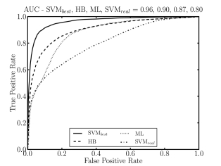
Ground-based optical surveys such as PanSTARRS, DES, and LSST, will produce large catalogs to limiting magnitudes of . Star-galaxy separation poses a major challenge to such surveys because galaxies—even very compact galaxies—outnumber halo stars at these depths. We investigate photometric classification techniques on stars and galaxies with intrinsic FWHM arcsec. We consider unsupervised spectral energy distribution template fitting and supervised, data-driven Support Vector Machines (SVM). For template fitting, we use a Maximum Likelihood (ML) method and a new Hierarchical Bayesian (HB) method, which learns the prior distribution of template probabilities from the data. SVM requires training data to classify unknown sources; ML and HB don’t. We consider i.) a best-case scenario (SVMbest) where the training data is (unrealistically) a random sampling of the data in both signal-to-noise and demographics, and ii.) a more realistic scenario where training is done on higher signal-to-noise data (SVMreal) at brighter apparent magnitudes. Testing with COSMOS data we find that HB outperforms ML, delivering completeness, with purity of for both stars and galaxies. We find no algorithm delivers perfect performance, and that studies of metal-poor main-sequence turnoff stars may be challenged by poor star-galaxy separation. Using the Receiver Operating Characteristic curve, we find a best-to-worst ranking of SVMbest, HB, ML, and SVMreal. We conclude, therefore, that a well trained SVM will outperform template-fitting methods. However, a normally trained SVM performs worse. Thus, Hierarchical Bayesian template fitting may prove to be the optimal classification method in future surveys.
1. Introduction
Until now, the primary way that stars and galaxies have been classified in large sky surveys has been a morphological separation (e.g., Kron, 1980; Yee, 1991; Vasconcellos et al., 2011; Henrion et al., 2011) of point sources (presumably stars) from resolved sources (presumably galaxies). At bright apparent magnitudes, relatively few galaxies will contaminate a point source catalog and relatively few stars will contaminate a resolved source catalog, making morphology a sufficient metric for classification. However, resolved stellar science in the current and next generation of wide-field, ground-based surveys is being challenged by the vast number of unresolved galaxies at faint apparent magnitudes.
To demonstrate this challenge for studies of field stars in the Milky Way (MW), we compare the number of stars to the number of unresolved galaxies at faint apparent magnitudes. Figure 1 shows the fraction of COSMOS sources that are classified as stars as a function of magnitude and angular size. The COSMOS catalog (() (237,43) degrees, Capak et al., 2007a; Scoville et al., 2007a; Ilbert et al., 2009) relies on 30-band photometry plus HST/ACS morphology for source classification (see Section 4 for details). In Figure 1 we plot separately relatively bluer () and redder () sources because bluer stars are representative of the old, metal-poor main sequence turnoff (MSTO) stars generally used to trace the MW’s halo while redder stars are representative of the intrinsically fainter red dwarf stars generally used to trace the MW’s disk. We will see that the effect of unresolved galaxies on these two populations is different, both because of galaxy demographics and because the number density of halo MSTO stars decreases at faint magnitudes while the number density of disk red dwarf stars increases at faint magnitudes.
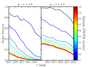
In an optimistic scenario in which galaxies with FWHM arcsec can be morphologically resolved (the blue line in Figure 1, second from the top), unresolved galaxies will still greatly outnumber field MW stars in a point source catalog. For studies of blue stars, field star counts are dominated by unresolved galaxies by and are devastated by unresolved galaxies at fainter magnitudes. The problem is far less severe for studies of red stars, which may dominate point source counts for . Although morphological identification of galaxies with FWHM as small as arcsec is better than possible for the Sloan Digital Sky Survey (median seeing arcsec), future surveys with higher median image quality (for example, arcsec predicted for LSST) may approach this limit.
Utilizing the fundamental differences between SEDs of stars and galaxies can mitigate the contamination of unresolved galaxies in point source catalogs. In general, stellar SEDs are more sharply peaked (close to blackbody) than galaxies, which exhibit fluxes more broadly distributed across wavelength. Traditionally, color-color cuts have been used to eliminate galaxies from point source catalogs (e.g., Gould et al., 1992; Reitzel et al., 1998; Daddi et al., 2004). Advantages of the color-color approach include its simple implementation and its flexibility to be tailored to the goals of individual studies. Disadvantages of this approach can include its simplistic treatment of measurement uncertainties and its limited use of information about both populations expected demographics.
Probabilistic algorithms offer a more general and informative approach to photometric classification. The goal of probabilistic photometric classification of an astronomical source is to use its observed fluxes to compute the probability that the object is of a given type. For example, a star () galaxy () classification algorithm produces the posterior probabilities and and decides classification by comparing the ratio of the probabilities
| (1) |
A natural classification threshold is an odds ratio, , of 1, which may be modified to obtain more pure or more complete samples.
Algorithmically there are a large number of approaches which produce probabilistic classifications. Generally, these fall into i) physically based methods—those which have theoretical or empirical models for what type of physical object a source is, or ii) data driven methods—those which use real data with known classifications to construct a model for new data. Physically based Bayesian and template fitting methods have been extensively used to infer the properties of galaxies (e.g., Coil et al., 2004; Ilbert et al., 2009; Xia et al., 2009; Walcher et al., 2011; Hildebrandt et al., 2010). However, in those studies relatively little attention has been paid to stars which contribute marginally to overall source counts (although see Robin et al. 2007). Several groups have recently investigated data driven, support vector machine based star–galaxy separation algorithms (e.g., Saglia et al., 2012; Solarz et al., 2012; Tsalmantza et al., 2012).
In this paper, we describe, test, and compare two physically based template fitting approaches to star–galaxy separation (maximum-likelihood and hierarchical bayesian), and one data driven (support vector machine) approach. In Section 2, we present the conceptual basis for each of the three methods. In Section 3, we describe the COSMOS data set with which we test the algorithms. In Section 4, we discuss the specific details, choices, and assumptions made for each of our classification methods. Finally, in Section 5 we show the performance of the algorithms, and discuss the advantages and limitations related to their use as classifiers.
2. Probabilistic Photometric Classification Techniques
2.1. Template Fitting: Maximum Likelihood (ML)
One common method for inferring a source’s properties from observed fluxes is template fitting. This method requires a set of spectral templates (empirical or theoretical) that span the possible spectral energy distributions (SEDs) of observed sources. These template SEDs must each cover the full wavelength range spanned by the photometric filters used to measure the fluxes to be fit. The relative template flux in each filter (for example ) for each SED is computed by convolving each SED with each filter response curve. Once these relative flux values are computed for each SED template, the template model is fully specified except for a normalization constant . For a given observed source , the value of is proportional to the total luminosity of the source divided by the luminosity distance squared. This value of is unknown but can be ‘fit’ to the data.
The maximum likelihood (ML) value of for each template that best fits a source’s observed fluxes, , is that which returns the lowest . After assessing the ML values of for all the templates, classification is straightforward—one need only to compare the lowest star to the lowest galaxy . In other words, is the classification criteria (see Equation 1).
2.2. Template Fitting: Hierarchical Bayesian (HB)
Hierarchical Bayesian (HB) algorithms provide another template fitting-based approach to photometric classification. Unlike ML approaches, Bayesian approaches offer the opportunity to utilize information about how likely a source is to be each kind of star or galaxy; the different templates are not treated as equal a priori. With a hierarchical Bayesian algorithm, individual source prior probabilities do not need to be set in advance of the full-sample classification process; the entire sample of sources can inform the prior probabilities for each individual source.
Consider the scenario where a model fits data only slightly better than the best model, while all other models give poor fits and all other models give nearly as likely fits. In this case, ignoring all other models besides the best is the wrong thing to do, since the data are stating that models are generally more favored. Capturing this kind of information is one primary aim of most Bayesian algorithms.
To capture this information, we marginalize over all possible star and galaxy templates to compute the total probability that a source belongs to a certain classification ( or ). For a template fitting-based Bayesian algorithm, this marginalization consists of summing up the likelihood of each template given , as well as the likelihood of each template (across redshift). Note that the likelihood of each template is itself calculated as a marginalized likelihood. For each template fit, we compute the total likelihood of the fit by marginalizing over the uncertainty in fitting coefficient . This marginalization is the total probability of a Gaussian distribution with variance —a value which is returned using least squares fitting techniques (e.g., Hogg et al., 2010a).
By Bayes’ theorem, marginalization requires we specify the prior probability that any object might have a given SED template (at a given redshift). The prior probability distributions might be chosen to be uninformative (for example, flat), informed by knowledge from outside studies, or informed by the data on all the other objects. The latter approach, referred to as a hierarchical model, is widely used in statistical data analysis (e.g., Gelman et al., 2003) and is beginning to be used in astronomy (Mandel et al., 2009; Hogg et al., 2010b; Mandel et al., 2011; Shu et al., 2012). The benefits of hierarchical approaches are many—because every inference is informed by every datum in the data set, they generally show improved probabilistic performance over simpler approaches, while requiring no additional knowledge outside the observed data and the template SEDs. Functionally, hierarchical approaches consist of parameterizing the prior probability distributions (for example, with the mean and variance of a Normal distribution), and varying these parameters (known as “hyperparameters”) to determine the probability of all the data under all the models.
For our work, we optimize the hyperparameters of the SED template prior distributions to return the maximum marginalized likelihood of all the data. This procedure will enable us to simultaneously infer the star–galaxy probability of each source while determining the hyperparameters that maximize the likelihood of the observed dataset. A brief description of the functional form of these priors is given below in Section 4.2. Although we focus on the star–galaxy probabilities in this paper, the optimized hyperparameters themselves yield a measurement of the detailed demographics of a dataset.
2.3. Support Vector Machine (SVM)
A support vector machine (SVM) is a type of machine learning algorithm particularly well suited to the problem of classification. SVM algorithms are frequently used in non-astronomical problems, and are considered a gold standard against which to compare any new classification method. SVM algorithms are “supervised”, meaning they train on a catalog of objects with known classifications to learn the high dimensional boundary that best separates two or more classes of objects. For classification problems which do not separate perfectly, SVMs account for misclassification errors by looking at the degree of misclassification, weighted by a user specified error penalty parameter. In general the optimal boundary need not be restricted to a linear hyperplane, but is allowed to be non-linear and so can require a very large number of parameters to specify the boundary. In order for non-linear SVM classification to be computationally feasible, a kernel function is used to map the problem to a lower dimensional feature space (Boser et al., 1992).
For the case of star–galaxy separation based on broad band photometry, the SVM algorithm learns the boundary which best separates the observed colors and apparent magnitudes111We use apparent magnitude here. of stars and galaxies. For more details on the SVM technique, please see Müller et al. (2001).
Successful implementation of a SVM algorithm requires a training dataset that is a sufficient analog to the dataset to be classified. A SVM has recently been applied to source classification in the Pan-STARRS 1 photometric pipeline (Saglia et al., 2012), with promising initial results. However, these results were obtained based on analysis of bright, high signal-to-noise data (), using training data which is a subset of the data itself.
To investigate the impact of training set quality and demographics on the problem of star–galaxy separation, we will consider the utility and performance of SVM algorithms in a new classification regime, where the data is of lower signal to noise (described in Section 3), and the number of unresolved galaxies is comparable to or larger than the number of stars.
3. Test Data
To investigate the advantages and disadvantages of star–galaxy classification techniques, we need a test catalog which has a large number of sources, is well understood and calibrated, and for which spectroscopy or multi-wavelength observations reveal the true source classifications. In addition, we want these data to be magnitude limited as faint as in order to understand the problem of classification in current and upcoming surveys like Pan-STARRS 1, DES, and LSST. The COSMOS catalog satisfies these requirements.
The COSMOS survey (Scoville et al., 2007b) covers 2 square degrees on the sky using 30 band photometry, and is magnitude limited down to . Broadband photometry exists down to limiting magnitudes which complement the limiting magnitude, and Spitzer IRAC coverage exist for sources as faint as (Capak et al., 2007b; Sanders et al., 2007; Taniguchi et al., 2007). In addition, GALEX and XMM coverage are of sufficient depth to pick out relatively bright star-forming galaxies and AGN (Hasinger et al., 2007; Zamojski et al., 2007). The spectral coverage beyond the optical, particularly the near-infrared, can be a powerful discriminator between star and galaxy classification. For instance, Ilbert et al. (2009) show the vs. colors cleanly separate star and galaxy loci, since stars have systematically lower colors. In addition to 30 band photometry, the COSMOS field has HST/ACS band coverage, down to a limiting magnitude of (Koekemoer et al., 2007; Scoville et al., 2007a). Diffraction limited HST imaging allows the morphological discrimination of point-like and extended sources, further strengthening the fidelity of the COSMOS star–galaxy classification.
We follow the COSMOS team’s star–galaxy classification criteria in order to determine the ‘true’ classification for the purpose of testing our methods. These consist of a classification from fitting star and galaxy templates to the 30 band photometry, and a morphological classification using the ACS_MU_CLASS statistic derived by the analysis of the HST photometry by Scarlata et al. (2007). We label COSMOS sources as stars if ACS_MU_CLASS says the source is pointlike, and the ‘star’ is lower than that for ‘AGN/QSO’. For galaxies, we require the source to have a non-pointlike ACS_MU_CLASS. This classification assumes that all galaxies in the HST images are resolved. We view this as an excellent approximation of the truth – COSMOS ACS images are very deep (), and can thus detect the faint extended features of nearly unresolved galaxies. We have qualitatively confirmed this by examining the distribution of galaxy FWHM, and find the distribution to be smoothly decreasing down to the smallest FWHM in the data. We estimate the number of galaxies labeled as stars to be below the few-percent level. For the labeling, we use an updated version of the publicly available photometric catalog, provided by P. Capak (private communication). While present in the catalog, we do not use any photometric redshift information in determining the classification of COSMOS sources.
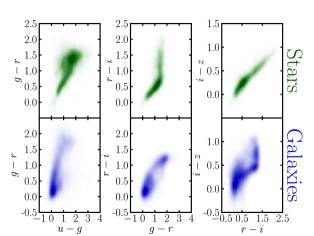
Throughout this paper, we restrict our analysis to sources likely to be unresolved in ground based data (FWHMHST/ACS arcsec). We do so since commonly used morphological classification criteria will easily distinguish quite extended sources, accounting for a majority of galaxies to depths of . However, galaxies with angular sizes arcsec are unlikely to be resolved in surveys with seeing arcsec, and so are an appropriate test bed for the type of sources which will rely the most on photometric star–galaxy separation. In total, our sample consists of 7139 stars and 9167 galaxies with apparent magnitudes , and is plotted in ugriz color–color space in Figure 2. Over this magnitude range, the median signal-to-noise in the band ranges from at to at , with lower corresponding ranges of 10 to 7 in the . Of all 18606 sources with FWHM arcsec in the COSMOS catalog, we identified 2300 AGN, which we discard from our current analysis.
4. Implementation of Three Star–Galaxy Classifiers
In this Section, we describe our implementation of ML template fitting, HB template fitting, and a SVM on the photometry of COSMOS sources for purposes of star–galaxy classification.
4.1. ML Template Fitting
Template based star–galaxy classification relies on the use of spectral energy distribution templates which (as well as possible) span the space of colors for both stars and galaxies. For our stellar model library, we first adopt the Pickles (1998) set of empirically derived SEDs, which span O to M type stars for both main sequence, giant, and supergiant stars. The vast majority of the SEDs in the Pickles library have solar abundances, so we supplement the library with theoretical SEDs from Castelli-Kurucz (CK) (Castelli & Kurucz, 2004). We use CK models with abundances ranging from [Fe/H], surface gravities ranging from , and effective temperatures from K. We include binary star templates by combining like-metallicity templates using flux calibrated CK models. Finally, we include SDSS M9 through L0 dwarf templates provided by J. J. Bochanski (private communication). These templates have been extended from the templates of Bochanski et al. (2007) into the near infrared, but lack data for wavelengths shorter than Å. We extend these templates down to the Å using a main sequence CK model with K. Details of this extension are likely to be unimportant, since the flux of such stars between Å is negligible. Our final combined library of stellar templates includes 131 from the Pickles library, 256 from the CK library, 11 from Bochanski et al. (2007), and 1319 binary templates constructed from the CK library, for a total of 1717 stellar templates.
We select for our galaxy templates those used by the COSMOS team, described in (Ilbert et al., 2009), provided publicly through the Le Phare photometric redshift package222 http://www.cfht.hawaii.edu/%7Earnouts/LEPHARE/lephare.html (Arnouts et al., 1999; Ilbert et al., 2006). These templates consist of galaxy SEDs from Polletta et al. (2007), encompassing 7 elliptical and 12 spiral (S0-Sd) SEDs. Additionally, 12 representative starburst SEDs are included, which were added by Ilbert et al. (2009) to provide a more extensive range of blue colors. Templates from Polletta et al. (2007) include effects of dust extinction, since they were selected to fit spectral sources in the VIMOS VLT Deep Survey (Le Fèvre et al., 2005). We do not consider any additional dust extinction beyond these fiducial templates. In order to model our galaxies across cosmic time, we redshift these templates on a discrete linear grid of redshifts, ranging from 0 to 4 in steps of 0.08. Simple tests using the ML procedure indicate small changes to the step size of our grid are unimportant.
For all of the above templates, model fluxes were constructed by integrating the SED flux density values with the throughput response curves for each filter. These consist of a response curve for the observations taken by the Canada-France-Hawaii Telescope, and , , , response curves for data collected by the Subaru telescope. We obtained the same response curves used by Ilbert et al. (2009) through Le Phare55footnotemark: 5. To check for any mismatch between the data, calibrations, and/or response curves, we verified that model colors generated from the SEDs overlap well with the star and galaxy loci.
4.2. HB Template Fitting
While the HB template fitting technique builds on the foundation described in Section 4.1, the details of star–galaxy inference require significantly more mathematical formalism to thoroughly describe. We present the details of this formalism and a detailed, step-by-step description of our HB inferential procedure in Appendix A. Open-source C code is available at http://github.com/rossfadely/star-galaxy-classification. In this section, we qualitatively describe features specific to our HB algorithm. We emphasize that hierarchical Bayesian algorithms are unsupervised: we use no training set and do not set priors in advance of running the algorithms. As described in Section 2.2, the priors for the templates are inferred from the data itself.
Our HB template fitting method draws from the same set of SED templates described above in Section 4.1. However, to speed up the algorithm, we used only 250 of the 1313 star templates, spanning a range of physical and color-color properties. In practice, we find the individual choice of these templates to be unimportant (since many are very similar) so long as the templates span the colors of stars, with a sampling close to or better than the typical color uncertainties of the data. We believe similar arguments to be true for galaxies, but have not explored such issues since we currently use only 31 galaxy templates.
The primary choice we must make for our HB approach is the functional form(s) of the prior probability distributions in the model. Since our templates are discrete both in SED shape and physical properties, we parameterize the prior probability of each template to be a single valued weight, within the range 0 to 1, such that the weights sum to 1 (see, for example, A9 and A10). These weights themselves become hyperparameters in our optimization. We thus have 281 hyperparameters corresponding to template priors since we use 250 star and 31 galaxy templates. The overall prior probability that any given object is or is also parameterized as two weights that sum to one (A13 and A14 in Appendix), which we optimize.
For the galaxy models, we must choose a form for our redshift priors. Ideally, these should be parameterized as weights for each discrete redshift, repeated as a separate set for each galaxy template. Unfortunately, this would not only add more hyperparameters to optimize, but also significantly slows down likelihood computations. Instead, we adopt a flat prior distribution across redshifts. While not ideal, such a prior eases comparison with ML classification results, and eliminates the need to specify an informative prior which correctly describes the data. Tests of flat versus fixed-form prior distributions indicate that the classification results presented in Section 5 do not vary substantially between the two choices.
Finally, for each template fit we marginalize over the (Gaussian) uncertainty in the fit amplitude, for which we must specify a prior distribution (A6 and A7 in Appendix). We adopt a log-normal prior for the fit amplitudes, which we set by taking the mean and variance of the log-amplitudes from fits of all the data for a given template. This approach makes the priors essentially uninformative, since the variance for all the data is large with respect to the variance for data which is well fit by the template. Like redshift priors, these too could be treated as hyperparameters but come at the cost of much slower likelihood computations.
In summary, we fix redshift and fit-amplitude priors and vary the prior weights of the template and probabilities. Thus, we optimize 283 prior (hyper)parameters to values which yield the maximum likelihood of the entire dataset.
4.3. SVM Models
We use the LIBSVM 333http://www.csie.ntu.edu.tw/%7Ecjlin/libsvm/— set of routines, described in Chang & Lin (2011). The provided routines are quick and easy to implement, and only require the user to specify a training set of data, a set of data to be classified (a.k.a., test data), and the form and parameter values of the kernel function used.
We employ a Gaussian radial basis function for the SVM kernel, for which we must specify a scaling factor . Together with the error penalty parameter () we have two nuisance parameters whose optimal values we need find. We do this by using a Nelder-Mead simplex optimization algorithm to find the parameter values which provide the highest number of correct classifications in the test data. In detail, the optimal values for will be different for each combination of training and test data.
To select the training data, we consider two scenarios. First is a ‘best case’ situation (SVMbest), where a well-characterized training set exists which is a fair sampling of the test data, with both the same object demographics and same signal-to-noise () as the data to be classified. To emulate this scenario, we select the training set as a random sample of the COSMOS catalog. Second, we consider a more realistic case where the available training set is only sampling the demographics of the high portion of the catalog to be classified (SVMreal). In this case, the demographics of objects in the training set may not match the demographics of the majority of objects in the set to be classified.
We consider SVMbest an optimistic scenario—obtaining a large spectroscopic or multi-wavelength sample of training data, down to the limiting magnitude of a given survey, is very costly in terms of telescope time. The other extreme, SVMreal, is a bit more realistic—for a given survey, classifications are typically easily obtained only at the high end of the data. In both cases, we consider a training sample size which is a fifth of the total catalog size.
Finally, to implement the SVM classification routine we need to scale both the training data and test data. That is, for the colors and apparent magnitude used, we must scale the range of each to lie between and . We map both training and test data to the interval using the full range of values in the test data. This is important in the case of SVMreal, since the training data may not span the full range of values for the test data. We find that scaling can have a significant effect for the SVMreal model. For example, poor classification performance is obtained if the SVMreal training data is scaled to itself rather than to the test data.
5. Results and Discussion
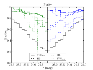
We report the classification performance of Maximum Likelihood (ML) and Hierarchical Bayesian (HB) template fitting, as well as a thoroughly tested Support Vector Machine (SVM) on our COSMOS based test data. There are many different measures which can be used to assess the performance of each algorithm. First, we consider the completeness444Defined as the fraction of sources of true type , correctly classified as . and purity555Defined as the number of sources of true type , correctly classified as , divided by the total number of sources classified as . of classified samples, evaluated at 666Defined in Equation 1. Figures 3 and 4, display the completeness and purity, respectively, as a function of magnitude. Examining Figure 3, all methods seem to be fairly competitive for galaxy classification, returning completeness across all magnitudes. SVMbest and ML yield the most consistently robust completeness for galaxies. In the case of stars, however, it is clear only our HB template fitting and SVMbest deliver acceptable completeness—at the completeness of ML template fitting falls to 50% or below, and the completeness for SVMreal goes to zero. The mismatch in source demographics between the realistic training set and the faint COSMOS sources severely undermines the efficacy of SVMreal.
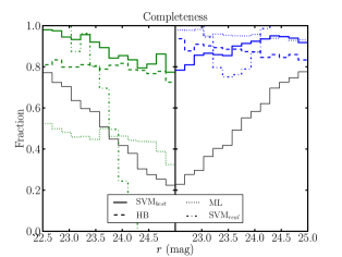
In terms of purity (Figure 4), SVMbest outperforms all other approaches. For stars, HB yields similar performance to SVMbest, but all approaches underperform SVMbest in terms of galaxy purity. When taken in concert with the results of Figure 3, we see that HB delivers similar or better performance than ML in all cases, even with the relatively simple HB approach presented here. For stars, ML and HB yield similar sample purity, but HB does so with a much higher completeness ( vs. ). For galaxies, HB yields a consistently higher sample purity by but a consistently lower sample completeness by .
We infer below that the performance achieved by the SVMbest algorithm may represent the best possible classification of stars and galaxies that could be done, based on single-epoch photometry alone. However, it is unlikely that an ideal training set will be available for object classification in future, deep datasets. Identifying the regions of ugirz color–color space where classification fails can highlight possible ways to improve the unsupervised HB (or ML) classification methods implemented here. For example, we want to check for regions of color-color space in which templates used in ML and HB may be missing, or to check whether the implementation of simple, but stronger, priors could increase performance.
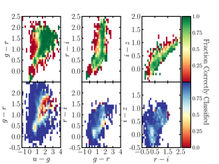
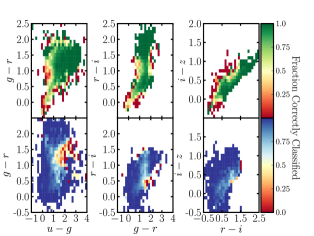
Figures 5 and 6 show the fraction of sources correctly classified using HB and SVMbest, distributed over colors. Comparing with Figure 2 reveals that the places where classification is least successful are regions where stars and galaxies overlap the most in color. For example, both the SVMbest and the HB algorithm struggle to correctly identify galaxies with 1 3 and 1 1.5. The number density of galaxies in the failing region is low, making HB even more likely to call everything a star. Similarly, both stars and galaxies populate and , presenting a challenge to both SVM and HB algorithms. In this case, the number density of galaxies is higher than that of stars, making HB even more likely to call everything a galaxy and training SVM on a color separation that favors galaxies over stars.
In the region of , the stellar locus has essentially zero overlap with galaxies in the sample. The SVMbest algorithm yields exquisite classification of these stars, while the HB algorithm returns only a mediocre performance (although and is populated with few stars, so those poorly classified regions do not represent a significant fraction of all stars). In future work, the classification of stars could therefore be improved with the implementation of stronger priors on the permitted redshifts at which galaxies may live—for example, by forcing a zero probability of elliptical galaxies at high redshifts.
Locating regions of color space in which the classifiers struggle to correctly separate stars and galaxies not only helps to decipher weaknesses in classification algorithms, but can be used to identify the specific science cases which will be most highly impacted. To illustrate, we examine places where both SVMbest and HB underperform and compare these regions to the object types in our templates. For stars we identify two such regions. The first lies within and , which has been suggested to be comprised of white dwarf, M dwarf binaries (Silvestri et al., 2006; Covey et al., 2007). The second region, with and , is consistent with metal-poor main-sequence turnoff stars. The relatively poorer performance in this region is particularly troubling, since these populations are some of the main tracers for low-surface brightness Galactic halo structure.
For galaxies, association of underperforming regions to specific populations is less clear-cut. For instance, we find the poor performing region with consistent with S0/SA SEDs with redshifts less than 0.4, but also with dusty starbursting galaxies across a wider redshift range. While far from comprehensive, these associations highlight the fact that classification performance can affect certain science cases more than others, and should be accounted for both during individual analyses and in future algorithm development.
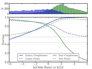
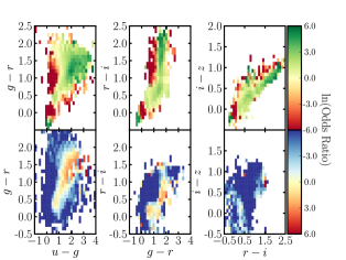
One of the great advantages of probabilistic classification is that one need not restrict the classification criterion to a fixed value. By moving away from , one can obtain more/less pure or complete samples of stars and galaxies, depending on the user’s science case. In detail, how the purity or completeness varies as a function of depends on the algorithm used. To illustrate, we show in Figure 7 how purity and completeness vary for the log odds ratio output by our HB algorithm. In the figure, as decreases, we are requiring that the relative likelihood that an object is a galaxy is much higher than that for a star. Similarly, as increases we are requiring objects be more stringently classified as a star. Thus, by moving away from we change the star/galaxy purity and completeness to the point where everything is called a star or galaxy, giving 100% complete samples with a purity set by the sample fraction. One caveat, however, is that modifying the threshold to achieve more pure samples may select objects which lie in particular regions in SED space. To illustrate, we show in Figure 8 the distribution of in color space.
We have considered the completeness and purity of sets of data classified as stars or galaxies (as a function of ) as one means of comparing different classification algorithms. A strength of this approach to quantifying the efficacy of classification algorithms is its transparent connection to different science requirements, in terms of purity and completeness. A weakness of this approach is the impossibility of selecting an overall “best” algorithm that presents an average over competing scientific requirements. For example, Figure 3 shows that compared to SVMbest, our HB method gives better completeness in stars but slightly worse completeness for galaxies—which performs better in general?
We assess the overall performance of the various classification algorithms using the Receiver Operating Characteristic (ROC) curve. A ROC curve is a plot of the true positive rate versus the false positive rate of a binary classifier, as the classification threshold () is varied. In Figure 9, we plot the ROC curve for all four classification approaches considered here. An ideal classifier has a true positive rate equal to one for all values of . Thus, the Area Under the Curve (AUC) statistic is an assessment of the overall performance of the classifier. There are several points worth noting in Figure 9. First, we find our HB approach to template fitting outperforms the ML approach. Considering our simple HB implementation is not very computationally demanding (tens of minutes on typical desktop computer), even a basic HB approach should always be preferred over the ML case. SVM algorithms, when trained with data which accurately capture the SED and properties of the entire data, generally perform much better than our current template fitting methods. This is not surprising, since template driven algorithms are never likely to have as complete models as something data driven. In reality, available training data will likely only capture the high end of the survey in question. As shown in Figure 9, a SVMreal scenario underperforms even ML template fitting, casting severe doubt onto the usefulness of SVM with ill-suited training information. Future surveys which intend to use supervised techniques, therefore, will have to carefully consider if alternate strategies for obtaining training data (e.g., Richards et al., 2012a, b) can outperform template fitting methods.
6. Conclusions
Imminent and upcoming ground-based surveys are observing large portions of the sky in optical filters to depths (), requiring significant amounts of money, resources, and person power. In order for such surveys to best achieve some of their science goals, accurate star–galaxy classification is required. At these new depths, unresolved galaxy counts increasingly dominate the number of point sources classified through morphological means. To investigate the usefulness of photometric classification methods for unresolved sources, we examine the performance of photometric classifiers using ugriz photometry of COSMOS sources with intrinsic FWHM arcsec, as measured with HST. We have focused our analysis on the classification of full survey datasets with broad science goals, rather than on the classification of subsets of sources tailored to specific scientific investigations.
Our conclusions are as follows:
-
•
Maximum Likelihood (ML) template fitting methods are simple, and return informative classifications. At , ML methods deliver high galaxy completeness () but low stellar completeness (). The purity of these samples range from , and are a strong function of the relative sample fraction.
-
•
We present a new, basic Hierarchical Bayesian (HB) approach to template fitting which outperforms ML techniques, as shown by the Receiver Operating Characteristic (ROC). HB algorithms have no need for training, and have nuisance parameters that are tuned according to the likelihood of the data itself. Further improvements to this basic algorithm are possible by hierarchically modeling the redshift distribution of galaxies, the SEDs of the input templates, and the distribution of apparent magnitudes.
-
•
Support Vector Machine (SVM) algorithms can deliver excellent classification, which outperforms template fitting methods. Successful SVM performance relies on having an adequate set of training data. For optimistic cases, where the training data is essentially a random sample of the data (with known classifications), SVM will outperform template fitting. In a more-realistic scenario, where the training data samples only the higher signal to noise sources in the data to be classified, SVM algorithms perform worse than the simplest template fitting methods.
-
•
It is unclear when, if ever, adequate training data will be available for SVM-like classification, HB algorithms are likely the optimum choice for next-generation classifiers.
-
•
A downside of a paucity of sufficient training data is the inability to assess the performance of both supervised (SVM) and unsupervised (ML, HB) classifiers. If knowing the completeness and purity in detail is critical to the survey science goals, it may be necessary to seek out expensive training/testing sets. Otherwise, users will have to select the best unsupervised classifier (HB here), and rely on performance assessments extrapolated from other studies.
-
•
Ground based surveys should deliver probabilistic photometric classifications as a basic data product. ML likelihoods are useful and require very little computational overhead, and should be considered the minimal delivered quantities. Basic or refined HB classifications require more overhead, but can be run on small subsets of data to learn the priors and then run quickly on the remaining data, making them a feasible option for large surveys. Finally, if excellent training data is available, SVM likelihoods should either be computed or the data should be made available. In any scenario, we strongly recommend that likelihood values, not binary classifications, should be delivered so that they may be propagated into individual analyses.
The future of astronomical studies of unresolved sources in ground based surveys is bright. Surveys like PanSTARRS, DES, and LSST will deliver data that, in conjunction with approaches discussed here, will expand our knowledge of stellar systems, the structure of the Milky Way, and the demographics of distant galaxies. We have identified troublesome spots for classification in single-epoch photometric data, which may hinder studies of M-giant and metal-poor main-sequence turnoff stars in the Milky Way’s halo. Future studies could improve upon our preliminary results by impleneting more-sophisticated prior distributions, by identifying crucial improvements needed in current template models or training data, or by pursuing complementary non-SED based classification metrics.
References
- Arnouts et al. (1999) Arnouts, S., Cristiani, S., Moscardini, L., Matarrese, S., Lucchin, F., Fontana, A., & Giallongo, E. 1999, MNRAS, 310, 540
- Bochanski et al. (2007) Bochanski, J. J., West, A. A., Hawley, S. L., & Covey, K. R. 2007, AJ, 133, 531
- Boser et al. (1992) Boser, B. E., Guyon, I. M., & Vapnik, V. N. 1992, in Proceedings of the fifth annual workshop on Computational learning theory, COLT ’92 (New York, NY, USA: ACM), 144–152
- Capak et al. (2007a) Capak, P. et al. 2007a, ApJS, 172, 99
- Capak et al. (2007b) —. 2007b, ApJS, 172, 99
- Castelli & Kurucz (2004) Castelli, F., & Kurucz, R. L. 2004, arXiv:0405087
- Chang & Lin (2011) Chang, C.-C., & Lin, C.-J. 2011, ACM Transactions on Intelligent Systems and Technology, 2, 27:1, software available at http://www.csie.ntu.edu.tw/~cjlin/libsvm
- Coil et al. (2004) Coil, A. L., Newman, J. A., Kaiser, N., Davis, M., Ma, C.-P., Kocevski, D. D., & Koo, D. C. 2004, ApJ, 617, 765
- Covey et al. (2007) Covey, K. R., et al. 2004, AJ, 134, 2398
- Daddi et al. (2004) Daddi, E., Cimatti, A., Renzini, A., Fontana, A., Mignoli, M., Pozzetti, L., Tozzi, P., & Zamorani, G. 2004, ApJ, 617, 746
- Gelman et al. (2003) Gelman, A., Carlin, J. B., Stern, H. S., & Rubin, D. B. 2003, Bayesian Data Analysis, Second Edition (Chapman & Hall/CRC Texts in Statistical Science), 2nd edn. (Chapman & Hall)
- Gould et al. (1992) Gould, A., Guhathakurta, P., Richstone, D., & Flynn, C. 1992, ApJ, 388, 345
- Hasinger et al. (2007) Hasinger, G. et al. 2007, ApJS, 172, 29
- Henrion et al. (2011) Henrion, M., Mortlock, D. J., Hand, D. J., & Gandy, A. 2011, MNRAS, 412, 2286
- Hildebrandt et al. (2010) Hildebrandt, H., et al. 2010, arXiv:1008.0658
- Hogg et al. (2010a) Hogg, D. W., Bovy, J., & Lang, D. 2010a, arXiv:1008.4686
- Hogg et al. (2010b) Hogg, D. W., Myers, A. D., & Bovy, J. 2010b, ApJ, 725, 2166
- Ilbert et al. (2006) Ilbert, O. et al. 2006, A&A, 457, 841
- Ilbert et al. (2009) Ilbert, O., et al. 2009, ApJ, 690, 1236
- Koekemoer et al. (2007) Koekemoer, A. M. et al. 2007, ApJS, 172, 196
- Kron (1980) Kron, R. G. 1980, ApJS, 43, 305
- Le Fèvre et al. (2005) Le Fèvre, O. et al. 2005, A&A, 439, 877
- Mandel et al. (2011) Mandel, K. S., Narayan, G., & Kirshner, R. P. 2011, ApJ, 731, 120
- Mandel et al. (2009) Mandel, K. S., Wood-Vasey, W. M., Friedman, A. S., & Kirshner, R. P. 2009, ApJ, 704, 629
- Müller et al. (2001) Müller, K.-R., Mika, S., Rätsch, G., Tsuda, K., & Schölkopf, B. 2001, IEEE Neural Networks, 12, 181
- Pickles (1998) Pickles, A. J. 1998, PASP, 110, 863
- Polletta et al. (2007) Polletta, M. et al. 2007, ApJ, 663, 81
- Reitzel et al. (1998) Reitzel, D. B., Guhathakurta, P., & Gould, A. 1998, AJ, 116, 707
- Richards et al. (2012a) Richards, J. W., et al., ApJ, 744, 192
- Richards et al. (2012b) Richards, J. W., et al., MNRAS, 419, 1121
- Robin et al. (2007) Robin, A. C., et al. 2007, ApJS, 172, 545
- Saglia et al. (2012) Saglia, R. P. et al. 2012, ApJ, 746, 128
- Sanders et al. (2007) Sanders, D. B. et al. 2007, ApJS, 172, 86
- Scarlata et al. (2007) Scarlata, C. et al. 2007, ApJS, 172, 406
- Scoville et al. (2007a) Scoville, N. et al. 2007a, ApJS, 172, 38
- Scoville et al. (2007b) —. 2007b, ApJS, 172, 1
- Shu et al. (2012) Shu, Y., Bolton, A. S., Schlegel, D. J., Dawson, K. S., Wake, D. A., Brownstein, J. R., Brinkmann, J., & Weaver, B. A. 2012, AJ, 143, 90
- Silvestri et al. (2006) Silvestri, N. M., et al. 2006, AJ, 131, 1674
- Solarz et al. (2012) Solarz, A. et al. 2012, ArXiv e-prints
- Taniguchi et al. (2007) Taniguchi, Y. et al. 2007, ApJS, 172, 9
- Tsalmantza et al. (2012) Tsalmantza, P. et al. 2012, A&A, 537, A42
- Vasconcellos et al. (2011) Vasconcellos, E. C., de Carvalho, R. R., Gal, R. R., LaBarbera, F. L., Capelato, H. V., Frago Campos Velho, H., Trevisan, M., & Ruiz, R. S. R. 2011, AJ, 141, 189
- Walcher et al. (2011) Walcher, J., Groves, B., Budavári, T., & Dale, D. 2011, Ap&SS, 331, 1
- Xia et al. (2009) Xia, L. et al. 2009, AJ, 138, 95
- Yee (1991) Yee, H. K. C. 1991, PASP, 103, 396
- Zamojski et al. (2007) Zamojski, M. A. et al. 2007, ApJS, 172, 468
Appendix A Hierarchical Bayesian Star–Galaxy Classification
In this appendix, we provide a detailed, step-by-step description of our Hierarchical Bayesian algorithm. First, let us define the data as the sets:
| (A1) |
where , is the observed magnitude and uncertainty in filter number for number of filters. One sequence for the filters corresponds to . The zeropoint, , is:
| (A2) |
where is the standard flux density spectrum (Vega or AB), and is the fraction of photons incident on the top of the atmosphere which are counted by the detector, as a function of wavelength.
Next, we generate a model for the data using the templates:
| (A3) |
where corresponds to the flux density of a given spectral template. Finally, we define a goodness of fit statistic:
| (A4) |
where is a constant unitless amplitude applied to the model for the fit (discussed more below as ). The variance , where is a few percent and represents a nuisance parameter which (in a global sense) accounts for error in the models as well as underestimates in . The value of from our template fitting is the fundamental quantity on which our inference procedure is based, as follows below.
We represent the hypothesis that an object is a star or a galaxy by “” or “” respectively. For a given object , we fit a set of templates corresponding to using the procedure outlined above. The likelihood of template and amplitude under the stellar hypothesis given the single observed data point is:
| (A5) |
where is the full set of observations of object and the associated noise model, and is defined in Equation A4. Note that the is not necessarily the best-fit value for but rather the obtained with template when it is given amplitude .
We could optimize this likelihood, but really we want to compare the whole model space to the whole model space. We must marginalize this likelihood over the amplitude and template. To demonstrate this, let us step through each marginalization for the model space.
Marginalization over the amplitude looks like
| (A6) |
where the integral is over all permitted values for the amplitude , and the prior PDF depends on the template , the full hypothesis . Note, the prior PDF obeys the normalization constraint
| (A7) |
Here we have also introduced some “hyperparameters” , which are variables which parameterize prior distributions. The subset of hyperparameters which apply to might be, for example, the mean and variance of a log-normal distribution on . It is the simultaneous inference of the star–galaxy probabilities and the hyperparameters that make the approach hierarchical.
Any realistic prior PDF for the comes from noting that (for stars), the are dimensionless squared distance ratios between the observed star and the template star; in this case the prior involves parameters of the stellar distribution in the Galaxy. When we look at galaxies (below), this situation will be different. In the (rare) case that the prior PDF varies slowly around the best-fit amplitude,
| (A8) |
where is the best-fit chi-squared, is the best-fit amplitude, and is the standard uncertainty in found by least-square fitting. This approximation is that the prior doesn’t vary significantly within a neighborhood of the best-fit amplitude.
Marginalization over the template space looks like
| (A9) |
where is the prior probability (a discrete probability, not a PDF) of template given the hypothesis and the hyperparameters . It obeys the normalization constraint
| (A10) |
Note is a discrete set of weights, whose value corresponds to the hyperparameter for template .
To summarize, the marginalized likelihood that a source is a star is computed as:
| (A11) |
The marginalized likelihood that source is a galaxy , is calculated following a very similar sequence. In calculating the likelihood, we allow a given galaxy template to be shifted in wavelength by a factor . This introduces another step in the calculation that marginalizes the likelihood across redshift for a template, giving
| (A12) |
where now is the constant amplitude for galaxy template at a redshift . The marginalization across redshift also introduces a prior , which is also is parameterized by a subset of , under some assumed form for the prior.
This model is fully generative; it specifies for any observed flux the PDF for that observation given either the star hypothesis or the galaxy hypothesis . We can write down then the full probability for the entire data set of all objects :
| (A13) |
where even the overall prior probability that an object is a star (or, conversely, a galaxy) depends on the hyperparameters . These obey the normalization constraint
| (A14) |
The likelihood is the total, marginalized likelihood for the combined data set of all the observations for all objects . From here we can take a number of approaches. One option is to find the hyperparameters that maximize this total marginalized likelihood, or we can assign a prior PDF on the hyperparameters, and sample the posterior PDF in the hyperparameter space. For computational reasons, we choose to optimize in this work.
With either a maximum-likelihood set of hyperparameters or else a sampling, inferences can be made. For our purposes, the most interesting inference is, for each object , the posterior probability ratio (or odds)
| (A15) |
where we have re-used most of the likelihood machinery generated (above) for the purposes of inferring the hyperparameters. That is, the star–galaxy inference and the hyperparameter inferences proceed simultaneously.