Acceptance corrections to net baryon and net charge cumulants
Abstract
We show that the effect of finite acceptance drastically influences the net-baryon and net-charge cumulants, which are believed to be sensitive probes of the QCD phase diagram. We derive the general formulae that relate the true cumulants which reflect the full dynamics of the system with the actually measured cumulants for a given acceptance, modeled by a binomial probability parameter . We find that this relation involves additional moments which cannot be expressed by cumulants and should be measured in order to extract any potential information about the QCD critical point. We demonstrate that for a wide range of the true cumulant ratios the measured ratios quickly converge if , which makes the interpretation of the data very challenging, especially in case of the net-proton cumulants. Our study further suggests that the measurement of net-charge cumulants may be more advantageous for the investigation of the QCD phase diagram.
pacs:
25.75.-q, 24.85.+p, 24.60.-kI Introduction
The exploration of the phase structure of Quantum Chromodynamics (QCD) has been a central topic in the study of the strong interactions for many years. Theoretically, the QCD phase diagram has been investigated with either effective models or by first principle Lattice QCD calculations. Experimentally, the phase structure of strongly interacting matter is studied with the help of relativistic heavy ion collisions. Experiments at the Relativistic Heavy Ion Collider (RHIC) and recent results from the Large Hadron Collider (LHC) have indicated that the collisions at the very highest energies produce a strongly interacting quark-gluon plasma at nearly vanishing net-baryon density.
Meanwhile Lattice QCD (LQCD) calculations have established that for vanishing net-baryon density the transition between the hadronic and partonic “phase” is an analytic cross over Aoki:2006we with a pseudo-critical temperature of Aoki:2006br ; Bazavov:2011nk . Therefore, true phase transitions, if at all present, will be located at finite values of the baryon density. Indeed, model calculations predict a first order coexistence region at high baryon density (several times nuclear matter density) and moderate temperatures, which ends in a critical point (for a compilation of various model results see, e.g., Stephanov:2007fk ). The precise location of this critical point, however, is not yet known from theory. Model calculations typically predict the location of the critical point to be at rather large values of the baryon number chemical potential, , which currently cannot be explored by Lattice QCD methods, due to the fermion sign problem.
Experimentally, the region of the phase diagram at finite density and moderate temperature is explored by heavy ion collisions at various energies. Freeze out points extracted from experiments range from values of nearly vanishing baryon chemical potential for LHC and top RHIC energies to values of at BraunMunzinger:2003zd . Since the location of the critical end point (CEP) is not really known the entire accessible region of the phase diagram needs to be explored by scanning the full range of available beam energies. Both the CEP as well as the first-order phase transition are associated with characteristic fluctuations – long range for the second-order transition at the CEP, and possible spinodal instabilities in case of a first order transition Sasaki:2007db ; Randrup:2009gp . Therefore fluctuations of various quantities such as particle multiplicities or mean transverse momentum have been proposed as suitable observables Stephanov:1999zu . Measurements of this sort have been carried out by the NA49 collaboration Alt:2008ca ; :2008vb at the CERN SPS and are also part of the recently started RHIC beam energy scan Aggarwal:2010wy . The first results by the NA49 collaboration Alt:2008ca ; :2008vb , which concentrated on the variances of various particle ratios and the transverse momentum, showed only very small deviations from the expected Poisson fluctuations of a Hadron Resonance Gas (HRG).
Meanwhile it has been realized that higher order cumulants would be more sensitive to the fluctuations associated with the second order transition, including the CEP Stephanov:2008qz ; Skokov:2010uh ; Stephanov:2011pb . The principle reason is that they scale with a higher power of the correlation length, which will be finite due to the rather short lifetime of the system created in these collisions. While the cumulants of many distributions may carry information about the CEP, theoretically the cumulants of the net-baryon number and of the net-charge are preferable since they are well defined as derivatives of the QCD partition function with respect to the appropriate chemical potentials. In addition, fluctuations of conserved quantities are less affected by final state interaction in the hadronic phase Koch:2008ia . Of course in an actual experiment, where the baryon number and electric charge of the entire system are conserved, corrections need to be applied to be able to compare with theoretical calculations which are typically carried out in the grand canonical ensemble, where charges are conserved only on the average. This point has been recently addressed, e.g., in Bzdak:2012an .
In addition to corrections due to charge conservation, in a real experiment one only observes a fraction of the final state particles. In case of the net-baryon distribution, typically the neutrons are not observed. Furthermore there are acceptance cuts as well as efficiency corrections for the protons, so that less than of baryons are actually observed. As we shall argue in this paper, this will lead to substantial corrections for the observed cumulants that need to be taken into account before any conclusions about critical fluctuations can be drawn. Specifically we will show that it is not sufficient to know the distribution of net-baryons (or net-charges) in order to predict the observed cumulants of the net-proton distribution. Instead, information for the full baryon/anti-baryon distribution, , is needed, which is not easily calculated in theory111In principle can only be calculated for systems where a quasi-particle description applies.. The same is true for the net-charge distribution, however in this case corrections are smaller since a larger fraction of charge particles are observed in a typical experiment. On the positive side, we will show that by measuring various factorial moments of the observed distribution one is able to extract the cumulants of the physical net-baryon distribution, , which is, after all, the desired goal.
We note that the question of acceptance corrections to various moments of particle distributions have already been discussed in the literature. For example corrections to the variance or second order cumulants of the net charge and net baryon number distributions have been investigated in Refs. Bleicher:2000ek ; Pruneau:2002yf ; Bower:2001fq , while acceptance effects on factorial moments have been addressed in Brooks:1996nu ; Kirejczyk:2004sc . Here we will concentrate on the corrections to higher order cumulants which are central to the discussion of the QCD critical point.
This paper is organized as follows. In the following section we will derive the relation between the cumulants of the underlying distribution to that of the actually measured distribution, and we will show that additional information other than cumulants is required. In the next section we will present some examples to illustrate the problems which arise if the acceptance corrections are large, as it is the case for the measurement of the net-baryon distribution. Before we conclude we will discuss a few observations pertinent to our results.
II Cumulants
Suppose we have an underlying probability distribution which captures the full dynamics of the system. Subsequently, we will refer to as the distribution within the “required acceptance”, where by required acceptance we mean that all particles that are necessary to capture the relevant physics are measured. This does not necessarily imply that all particles in the final state need to be measured.222To which extent an actual experiment does have the “required acceptance” is not easy to tell and naturally depends on the specific physics under consideration. Here and stand for either baryons and anti-baryons, i.e., and or positively and negatively charged particles, i.e., and . Let further be the net-baryon or net-charge cumulants associated with the underlying distribution . Of course in a real experiment additional cuts such as in the transverse momentum or rapidity will have to be applied. In addition, the efficiency to detect particles will be smaller that (in case of neutrons it is typically zero). To reflect this let us introduce the probability distribution of the actually observed multiplicities and . Let us further denote the net-baryon or net-charge cumulants of by . Finally, we assume that all acceptance corrections may be modeled by a binomial probability distribution333In reality, more sophisticated models than the binomial distribution are likely required to properly address the various acceptance corrections (see e.g. Pruneau:2002yf ). However, using the binomial distribution will illustrate the essential issues related with acceptance corrections.
| (1) |
The parameters and describe all possible acceptance effects in our system. For example, the detector acceptance is naturally modeled by the binomial distribution and it can be different for different particles. Additional cuts in the transverse or/and longitudinal momenta also introduce acceptance correction. In the context of the cumulants of the net-baryon distribution, it has been argued in Refs. Kitazawa:2011wh ; Kitazawa:2012at that the fact that neutrons are not observed in a typical experiment may also be modeled by a binomial distribution. Thus, Eq. (1) applies as well. Finally, we note that the different sources of limited acceptance can be represented by an effective parameter, which is simply the product of all binomial probabilities. For example, in case of the net-proton distribution: (number of protons), (number of anti-protons), see Eq. (1), and
| (2) |
where represents the fact that only protons are measured instead of baryons (), characterizes the cut in momentum for measured protons, is a detector efficiency for protons in a given momentum cut, and so on. Similar relation holds for .
In order to proceed it is convenient to introduce the factorial moments:
| (3) | ||||
| (4) |
Using Eq. (1) it is straightforward to show (see e.g. Brooks:1996nu ; Kirejczyk:2004sc ):
| (5) |
The next step is to express the cumulants of the distribution in terms of the factorial moments . Using the relation, Eq. (5), we can then write in terms to the measured factorial moments for given acceptance parameters and . Finally can be expressed by the cumulants , which will allow us to relate to . However, as we shall see below, the factorial moments and in general cannot be solely expressed in terms of the cumulants of the net distributions, and , respectively. Additional terms, not related to cumulants will arise.
It is useful to define the moment generating function:
| (6) | |||||
where [see Eq. (1)] and is the net multiplicity distribution
| (7) |
Equation (6) allows to calculate the cumulant generating function
| (8) |
For in Eqs. (6,8) we obtain the moment- and the cumulant generating function, , of the net multiplicity distribution . By definition, the cumulants and read:
| (9) |
The above equations allow us to calculate the cumulants and . To obtain the relation between them is straightforward but tedious. For instance both and contain [see Eq. (3)], so we express by and substitute into the expression for . In this way we can relate cumulants by cumulants and the factorial moments .
First, let us relate the measured cumulants with the cumulants of the underlying distribution . Here we present the results up to and we assume . In the Appendix we give the general relations up to Friman:2011pf (see also Schaefer:2011ex ; Gavai:2003mf ) with an arbitrary and . We obtain
| (10) | ||||
| (11) | ||||
| (12) |
and more complicated:
| (13) | |||||
To simplify the notation we have introduced
| (14) |
As can be seen from the above equations it is impossible to relate the cumulants solely with the cumulants and the parameter . In Eq. (11) the value of is present. In the information about and is needed. In Eq. (13) , and mixed factorial moments and appear. As already discussed in the introduction, these additional terms would have to be calculated in a given theory, in order to make a reliable predictions for the measured cumulants . In general this is difficult and likely can only be done if a quasi-particle description for the dynamics applies.
It is interesting to consider two limits of : for we obviously obtain , and for very small the following relations hold
| (15) |
where . In the limit the ratios of cumulants read: , . It means that even if the cumulant ratio contains information about the QCD phase diagram (or any other interesting physics) this information is lost if the acceptance is too small. In other words in the limit the Skellam distribution is obtained, i.e., we are in the limit of Poisson statistics.
To summarize, Eqs. (10-13) allow to obtain the values of cumulants at a given acceptance parameter , knowing the cumulants and certain factorial moments of the underlying distribution . This distribution according to our assumptions is obtained for the “required acceptance”, defined by .
In practice, the more interesting question is to which extent one can express the cumulants , which contain the relevant physics, in terms of the measurable cumulants, , and factorial moments, . Actually this can be easily done using Eqs. (10-13) and the relation (5):
| (16) | ||||
| (17) | ||||
| (18) |
and
| (19) | |||||
where we introduced the notation
| (20) |
These equations can be directly used to extract the values of the true cumulants that characterize the system with , which we assumed to capture the relevant physics. We repeat: The measurement of the cumulants is not sufficient to extract the desired cumulants . The additional measurement of various factorial moments is required as well.
For example, in the context of the net-baryon fluctuations, denote the net-baryon cumulants. To determine all we need as input is the value of the acceptance parameter , the measured cumulants of the net-proton distribution, and the factorial moments measured for protons and anti-protons.
III Examples
In the following we present a few examples where we show the relation between the observed cumulants and the cumulants of the underlying distribution, . These are merely examples to illustrate the situation and certain assumptions about the necessary factorial moments will have to be made.
III.1
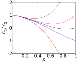
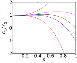
As an example we show the dependence of the ratio as a function of the acceptance parameter for different values of . As seen from Eq. (12), depends only on cumulants and and factorial moments and . To proceed we denote
| (21) |
where and is a free parameter that allows to change the widths of the distributions and 444For simplicity we assume that is the same for and multiplicity distributions.. Substituting Eq. (21) to Eq. (12) and using Eq. (10), we obtain:
| (22) |
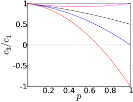
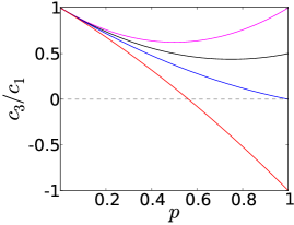
In the context of the net-baryon fluctuations it is expected that the width of the baryon (anti-baryon) distribution is comparable to the Poisson distribution Aggarwal:2010wy , that is . However, when net-charge fluctuations are studied the parameter is expected to be of the order of one 555The charge multiplicity distribution in heavy-ion and proton-proton collisions can be described by the negative binomial distribution, see, e.g., Adare:2008ns .. In Fig. 1 and Fig. 2 we present the dependence of as a function of for four values of , and , and we note that, as previously discussed, equals to the value of at . In Fig. 1 we assume that the multiplicity distribution is narrower than the Poisson distribution: in the left plot, and in the right plot.
In Fig. 2 we choose to be positive, i.e., the multiplicity distribution is broader than the Poisson distribution: in the left plot, and in the right plot.
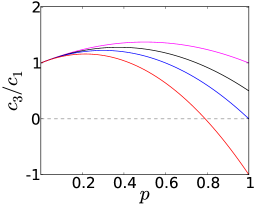
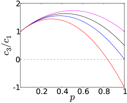
In case of net-baryon fluctuations the fact that we only measure protons (anti-protons) instead of all baryons (anti-baryons) already introduces . In addition finite detection efficiencies and cuts in the transverse momentum reduce the value of even more. We estimate that for the STAR measurement Aggarwal:2010wy the parameter may not be far from reality (assuming that the cut in rapidity is good enough to capture the relevant physics, and its contribution to can be neglected). As seen in Figs. 1 and 2 already the value of shifts the observed ratio into positive values even if is negative. Moreover, for different values of the values of quickly converge which makes the interpretation of the experimental results challenging. Taking a more realistic value of we see that it is practically impossible to distinguish between different values of , unless .
III.2
It is interesting to repeat the same exercise for . However, in this case we need additional information about , and the mixed factorial moments and . We investigated different values of parameters and we obtain similar plots as in Figs. 1 and 2. To present a few examples, we will assume that 666We note that this choice corresponds to a system at zero baryon chemical potential in the context of the net-baryon cumulants. However, the formalism presented in this paper is not restricted to this choice. Also, the corrections shown here are expected to be similar in case of finite chemical potential., and introduce the following parametrization
| (23) | |||||
| (24) | |||||
| (25) |
Equations (23,24) result from the assumption that is given by the negative binomial distribution. The parameter is identical as in Eq. (21), and controls the width of the multiplicity distribution. reflects the correlation between and . To further reduce the number of parameters we assume that 777We checked that modifications of this assumption do not introduce any new qualitative features.:
| (26) |
Finally, the value of is determined from the ratio that is an input in our calculation.
In Fig. 3 and Fig. 4 we present the dependence of as a function of the acceptance parameter for five values of and . In Fig. 1 we assume , see Eq. (14), and . In the left plot , and in the right one .
In Fig. 4 we assume and . In this case the multiplicity distribution is broader than Poisson, which is expected if the net-charge cumulants are investigated. In the left plot , and in the right one .
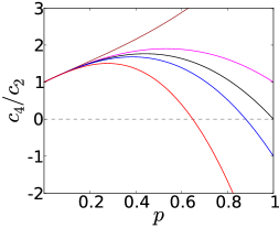
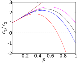
As seen from Figs. 3 and 4 the convergence of for various values of is even more rapid than in case of . Taking , as in the STAR measurement of net-proton cumulants, we see that even if there is any information about the QCD phase diagram in the net-baryon cumulants, this information is strongly diluted if only protons and anti-protons are measured.888Our finding naturally explains the large difference between net-baryon and net-proton cumulants observed in the UrQMD model Schuster:2009jv . At all lines are practically indistinguishable, unless (it should be of the order of ).
IV Comments
Let us discuss a few observations pertinent to the results from the previous sections:
(i) We demonstrated that a limited acceptance 999In particular the difficulty in measuring neutrons in the context of net-baryon fluctuations. makes a direct interpretation of measurements of higher order cumulants very difficult. Instead, we propose that the measurement of additional factorial moments, as shown in Eqs. (16-19), or the more general ones in the Appendix, is the way to proceed. This allows a rather unambiguous determination of the true cumulants .
(ii) The main problem with the measurement of the net-proton fluctuations is that the maximal value of is approximately .101010Of course if one compares with theoretical predictions which directly calculate the proton cumulants, such as Athanasiou:2010kw , the effective binomial probability is closer to one, similar to that for charged particles. However, it is not clear how to determine the proton cumulants in a model independent way. Moreover, additional cuts in the transverse momentum are usually needed. Also detection efficiencies are never . As a result, which makes the interpretation of the data very challenging. Even if one measured the additional factorial moments as proposed in this paper, their contribution becomes large for small values of [see Eqs. (16-19)] and thus need to be determined very precisely. This clearly favors the analysis of net-charge fluctuations, where there is no problem equivalent to the neutrons. Thus the parameter will likely be larger than and the extrapolation to the full acceptance by measuring the necessary factorial moments will be much more reliable. The cumulants of the net-charge fluctuations should also be sensitive to the CEP, however with a potentially smaller overall magnitude Stephanov:2008qz .
(iii) For the purpose of this paper, we have assumed that the “required acceptance”, i.e., , captures the relevant physics. To which extent this is the case for an actual experiment, such as STAR, is not clear and difficult to estimate. For example, it is not clear to us what the size of the rapidity window should be, in order to capture the relevant physics. One estimator would be the width of a thermal fireball, which is of the order of one unit of rapidity. However, it may very well be larger, and, therefore, the true value of may very well be smaller than in the STAR measurement.
(iv) Given the expression for the true cumulants in terms of the measured cumulants and factorial moments, Eqs. (16-19), it may be conceivable that one could explore the necessary rapidity range experimentally. As one increases the rapidity window the resulting should approach an asymptotic value once the window captures the relevant physics. On the other hand, doing the same exercise with the measured cumulants only may lead to false conclusions, especially in case of the net-proton distribution. Since the binomial parameter is already very small reducing the rapidity window will only lead to small variations (see Figs. 1-4) suggesting that the physics does not change.
(v) In our examples for we find that the choice for the correlation term in Eq. (25) leads to significant corrections for the measured cumulant ratio. Therefore, these correlation terms need to be measured precisely and we expect them to play an even stronger role in higher order cumulant ratios, such as .
(vi) We note the formalism presented here may be applied to higher order cumulants, such as , in a straightforward but tedious way (see Appendix). We believe that the problem to resolve the true cumulants gets even more difficult, the higher the order of the cumulant under consideration is.
(vii) Instead of measuring the cumulants one may consider other moments which are independent of the (binomial) acceptance corrections. For example the scaled factorial moments Pruneau:2002yf ; Brooks:1996nu ; Kirejczyk:2004sc , , see Eqs. (3, 4), would be such an alternative. Or one could construct combinations of moments similar to the one suggested in Bower:2001fq for the second moments. While these alternative moments should in principle carry similar information as the cumulants, they are not fully determined by the net-baryon distribution, . Therefore, a theoretical determination of these moments, e.g. from Lattice QCD, will necessarily require some model-dependent assumptions.
V Conclusions
In this paper we have studied the effect of finite acceptance on higher order cumulants of net-baryon and net-charge distributions. To this end we have folded the true probability distribution with binomial distribution in order to simulate the finite acceptance corrections. Our main finding is that the task of extracting the cumulants of the true distribution requires the measurement of not only the cumulants of the measurable distribution but in addition of various factorial moments, which cannot be expressed in terms of cumulants. We also demonstrated that for various values of the true cumulants ratios the measured ratios quickly converge with decreasing acceptance parameter . This makes the physical interpretation of the net-proton cumulants very difficult. We further argued that it may be advantageous to investigate the cumulants and factorial moments of the net-charge distribution, since in this case acceptance corrections are considerably smaller than for the net-baryon distribution. This may allow for a more reliable extraction of the true cumulants via the methods presented in this paper.
VI Acknowledgments
A.B. was supported by Contract No. DE-AC02-98CH10886 with the U. S. Department of Energy. V.K. was supported by the Office of Nuclear Physics in the US Department of Energy’s Office of Science under Contract No. DE-AC02-05CH11231. A.B. also acknowledges the grant N N202 125437 of the Polish Ministry of Science and Higher Education (2009-2012).
Appendix A General relations
Here we present the general relations between cumulants characterized by the “required acceptance”, and the measurable factorial moments at a given acceptance parameters and . As seen in Eqs. (17-19) it is not possible to express cumulants solely by cumulants but also factorial moments appear. Therefore, here we express solely by the factorial moments . This significantly simplifies our notation but makes no difference for an experimental application. We obtain
| (27) | ||||
| (28) | ||||
| (29) | ||||
| (30) |
and and are more complicated
| (31) |
and
| (32) |
In the above equations all cumulants can be directly measured due to the equality:
| (33) |
and
| (34) | ||||
| (35) |
References
- (1) Y. Aoki, G. Endrodi, Z. Fodor, S. D. Katz, and K. K. Szabo, Nature 443, 675 (2006), hep-lat/0611014.
- (2) Y. Aoki, Z. Fodor, S. D. Katz, and K. K. Szabo, Phys. Lett. B643, 46 (2006), hep-lat/0609068.
- (3) A. Bazavov et al., Phys. Rev. D 85, 054503 (2012) [arXiv:1111.1710 [hep-lat]].
- (4) M. A. Stephanov, PoS LAT 2006, 024 (2006) [hep-lat/0701002].
- (5) P. Braun-Munzinger, K. Redlich and J. Stachel, “Particle production in heavy ion collisions,” In *Hwa, R.C. (ed.) et al.: Quark gluon plasma* 491-599 [nucl-th/0304013].
- (6) C. Sasaki, B. Friman, and K. Redlich, Phys. Rev. Lett. 99, 232301 (2007), hep-ph/0702254.
- (7) J. Randrup, Phys. Rev. C79, 054911 (2009), arXiv:0903.4736.
- (8) M. A. Stephanov, K. Rajagopal, and E. V. Shuryak, Phys. Rev. D60, 114028 (1999), hep-ph/9903292.
- (9) NA49 Collaboration, C. Alt et al., Phys. Rev. C79, 044910 (2009), arXiv:0808.1237.
- (10) NA49 Collaboration, T. Anticic et al., Phys.Rev. C79, 044904 (2009), arXiv:0810.5580.
- (11) M. M. Aggarwal et al. [STAR Collaboration], Phys. Rev. Lett. 105, 022302 (2010) [arXiv:1004.4959 [nucl-ex]].
- (12) M. A. Stephanov, Phys. Rev. Lett. 102, 032301 (2009) [arXiv:0809.3450 [hep-ph]].
- (13) V. Skokov, B. Friman and K. Redlich, Phys. Rev. C 83, 054904 (2011) [arXiv:1008.4570 [hep-ph]].
- (14) M. A. Stephanov, Phys. Rev. Lett. 107, 052301 (2011) [arXiv:1104.1627 [hep-ph]].
- (15) V. Koch, Landolt Boernstein I/23, 8 (2010), arXiv:0810.2520.
- (16) A. Bzdak, V. Koch and V. Skokov, arXiv:1203.4529 [hep-ph].
- (17) M. Bleicher, S. Jeon and V. Koch, Phys. Rev. C 62, 061902 (2000) [hep-ph/0006201].
- (18) C. Pruneau, S. Gavin and S. Voloshin, Phys. Rev. C 66, 044904 (2002) [nucl-ex/0204011].
- (19) D. Bower and S. Gavin, Phys. Rev. C 64, 051902 (2001) [nucl-th/0106010].
- (20) T. C. Brooks et al. [MiniMax Collaboration], Phys. Rev. D 55, 5667 (1997) [hep-ph/9609375].
- (21) M. Kirejczyk, Acta Phys. Polon. B 35, 2425 (2004) [nucl-ex/0406029].
- (22) M. Kitazawa and M. Asakawa, Phys. Rev. C 85, 021901 (2012) [arXiv:1107.2755 [nucl-th]].
- (23) M. Kitazawa and M. Asakawa, Phys. Rev. C 86, 024904 (2012) [arXiv:1205.3292 [nucl-th]].
- (24) B. Friman, F. Karsch, K. Redlich and V. Skokov, Eur. Phys. J. C 71, 1694 (2011) [arXiv:1103.3511 [hep-ph]].
- (25) B. J. Schaefer and M. Wagner, Phys. Rev. D 85, 034027 (2012) [arXiv:1111.6871 [hep-ph]].
- (26) R. V. Gavai and S. Gupta, Phys. Rev. D 68, 034506 (2003) [hep-lat/0303013].
- (27) A. Adare et al. [PHENIX Collaboration], Phys. Rev. C 78, 044902 (2008) [arXiv:0805.1521 [nucl-ex]].
- (28) T. Schuster, M. Nahrgang, M. Mitrovski, R. Stock and M. Bleicher, arXiv:0903.2911 [hep-ph].
- (29) C. Athanasiou, K. Rajagopal and M. Stephanov, Phys. Rev. D 82, 074008 (2010) [arXiv:1006.4636 [hep-ph]].