PRISMA: PRoximal Iterative SMoothing Algorithm
Abstract
Motivated by learning problems including max-norm regularized matrix completion and clustering, robust PCA and sparse inverse covariance selection, we propose a novel optimization algorithm for minimizing a convex objective which decomposes into three parts: a smooth part, a simple non-smooth Lipschitz part, and a simple non-smooth non-Lipschitz part. We use a time variant smoothing strategy that allows us to obtain a guarantee that does not depend on knowing in advance the total number of iterations nor a bound on the domain.
1 Introduction
We propose an optimization method (PRISMA — PRoximal Iterative SMoothing Algorithm) for problems of the form111All the theorems hold also in general Hilbert spaces, but for simplicity of exposition we consider a Euclidean setting.:
| (1.1) |
where:
-
•
is a convex and -smooth function, that is, differentiable with a Lipschitz continuous gradient: .
-
•
is a convex -Lipschitz continuous function: .
-
•
is a proper, lower semicontinuous, convex (but possibly non-continuous/non-finite) function. For example, could be an indicator function for a convex constraint.
We further assume that we can calculate gradients of , and that and are “simple” in the sense that we can calculate their proximity operators222For more clarity here we explicitly define the proximity operator as a function of too because our algorithm heavily depends on this parameter changing over time.:
| (1.2) |
where , , and similarly for . That is, our method can be viewed as a black-box one, which accesses and only through the gradients of and the proximity operators of and . Each iteration of PRISMA requires one evaluation of each of , and and a few vector operations of overall complexity , and after such iterations we have
| (1.3) |
Applications.
Our main motivation for developing PRISMA was for solving optimization problems involving the matrix max-norm (aka norm). The max-norm has recently been shown to possess some advantages over the more commonly used trace-norm Lee et al. (2010); Jalali and Srebro (2012); Foygel and Srebro (2011), but is lagging behind it in terms of development of good optimization approaches—a gap we aim to narrow in this paper. Both norms are SDP representable, but standard SDP solvers are not applicable beyond very small scale problems. Instead, several first-order optimization approaches are available and commonly used for the trace-norm, including singular value thresholding Cai et al. (2008) and other Jaggi and Sulovsky (2010); Ma et al. (2009); Tomioka et al. (2010). However, until now there have been no practical first-order optimization techniques available for the max-norm. In Sec. 4 we show how max-norm regularized problems can be written in the form (1.1) and solved using PRISMA, thus providing for the first time an efficient and practical first order method for max-norm optimization.
We also demonstrate how PRISMA can be applied also to other optimization problems with complex structure, including robust principal component analysis (robust PCA), sparse inverse covariance selection and basis pursuit. In particular, for robust PCA, we show how PRISMA yields better performance then previously published approaches, and for basis pursuit we obtain the best known convergence rate using only first-order and proximity oracles.
Our Approach. Following ideas of Nesterov Nesterov (2005b) and others, we propose to smooth the function and use its proximity operator to obtain gradients of its smoothed version. However, unlike Nesterov (2005b), where a fixed amount of smoothing is used throughout the run, we show how to gradually change the amount of smoothing at each iteration. We can then use an accelerated gradient descent approach on plus the smoothed version of , as in Nesterov (2005b). We also use the ideas of partial linearization to handle the component : instead of attempting to linearize it as in gradient descent, we include it as is in each iteration, as in FOBOS Duchi and Singer (2009) and ISTA/FISTA Beck and Teboulle (2009). The gradual smoothing allows us to obtain a guarantee that does not depend on knowing in advance the total number of iterations, needed in Nesterov (2005b), nor a bound on the domain, needed in Nesterov (2005b); Chambolle and Pock (2011), and paying only an additional factor.
Notation. We use to denote the Fenchel conjugate, the indicator of the set (zero inside and infinite outside), the set of positive definite matrices, and the set of p.s.d. ones.
2 Smoothing of Nonsmooth Functions
As was suggested by Nesterov (2005a, b) and others, in order to handle the non-smooth component , we approximate it using a smooth function. Such a smoothing plays a central role in our method, and we devote this section to carefully presenting it. In particular, we use the -Moreau envelope Bauschke and Combettes (2011), known also as Moreau-Yosida regularization. For a function , the Moreau envelope , where , is defined as
| (2.1) |
The function is a smooth approximation to (in fact, the best possible approximation of bounded smoothness), as summarized in the following Lemmas:
Lemma 2.1 (Proposition 12.29 in Bauschke and Combettes (2011)).
Let be a proper, lower semicontinuous, convex function and . Then is -smooth and its gradient can be obtained from the proximity operator of as: .
Lemma 2.2.
Let a convex, -Lipschitz function, then
-
1.
if , then ;
-
2.
if , then .
Proof.
The proof extends the one of Lemma 2.5 in Shalev-Shwartz et al. (2010) to vectorial functions. Define . We have , and this proves the left hand side of the first property. For the other side of the inequality, we have
| (2.2) |
where we have used the Lipschitz property of . Hence
| (2.3) |
The second property follows from the first one and (Proposition 12.22 in Bauschke and Combettes (2011)). ∎
These two lemmas show how to obtain a smooth approximation of a Lipschitz continuous function, with the tradeoff between the smoothness and the degree of approximation controlled by the Lipschitz constant of the non-smooth function. Furthermore, in order to be able to work with the smoothed approximation , and in particular calculate its gradients, all that is required is access to the proximity operator of the non-smooth function . This is the reason we require access to .
Relation to Nesterov Smoothing. The Moreau envelope described above also underlies Nesterov’s smoothing method Nesterov (2005b), although his derivation is somewhat different. Nesterov refers to a non-smooth function that can be written as:
| (2.4) |
where , is a bounded closed convex set, and proposes to smoothen the function , where is a linear operator, with , where:
| (2.5) |
with , , and . The smoothness and approximation properties of are then given in terms of the diameter of the set , the parameter and a certain norm of the matrix . Any convex function can indeed be written in the form (2.4), where is its convex conjugate and is the set of all subgradients of — the diameter of thus corresponds to the Lipschitz constant (bound on the magnitude of the subgradients) of . Focusing on being the identity and (i.e. ), we have that defined in (2.5) is exactly the Moreau envelope :
Proposition 2.3.
If is a proper, lower semicontinuous convex function, is its Fenchel conjugate, the set of all its subgradients and , then .
This is obtained as a corollary from a slightly more general Lemma:
Lemma 2.4.
If is a proper, lower semicontinuous convex function which can be written as (2.4) and , then , where is the infimal convolution of and .
Proof.
Nesterov’s formulation is somewhat more general, allowing for different regularizers and different sets , but our presentation is a crisper and more direct statement of the assumptions on the function to be smoothed and its relationship to : we just need to be able to calculate the proximity operator of , to obtain gradients of , and we need to rely on its Lipschitz constant in order to be able to control the quality of the approximation.
3 PRoximal Iterative SMoothing Algorithm
Our proposed method, PRISMA, is given as Algorithm 1. As is standard in “accelerated” first order methods (e.g. Beck and Teboulle (2009)), we keep track of two sequences of iterates, and . At each iteration we perform a proximal gradient update , where the gradient of is calculated according to Lemma 2.1 and is some sequence of parameters. We then set to be a linear combination of and . Note also that the recursive formula for the sequence satisfies
| (3.1) |
We establish the following guarantee on the values of the objective function.
Theorem 3.1.
If the sequence is nonincreasing, then the iterates of Algorithm 1 satisfy, ,
| (3.2) |
In the following we show two possible ways to set the sequences . One possibility would be to decide on a fixed number of iterations and to set to a constant value.
Corollary 3.2.
For a given set . Then for every
| (3.3) |
This choice is optimal if we know the number of iterations we will use, as well as the Lipschitz constant and a bound on the distance from a minimizer, sharing the same limitation with Nesterov (2005b). But with this fixed choice of smoothing, even if we perform additional iterations, we will not converge to the optimum of our original objective (only of the smoothed, thus approximate, objective).
We propose a dynamic setting of , that gives a bound that holds uniformly for any number of iterations, and thus a method which converges to the optimum of the original objective.
Corollary 3.3.
Let and set in Algorithm 1, then, uniformly for any and for every
| (3.4) |
Proof.
It is easy to derive that (by induction) and the elementary chain of inequalities . The assertion then follows from Theorem 3.1 and these facts. ∎
Note that the optimal choice of does depend on the Lipschitz constant and on the distance of our initial point from a minimizer, but that the algorithm does converge for any choice of . Thus, compared to the bound in Corollary 3.2, the price we pay for not knowing in advance how many iterations will be needed is only an additive logarithmic factor333Ouyang and Gray (2012a) use a similar proof technique, for the simpler case when , and they report a convergence rate bound without the logarithmic term. Unfortunately their proof contains an error; they fixed it in the arxiv version of their paper Ouyang and Gray (2012b). Their new theorem contains the term , which is not known how it can be bounded..
When the updates reduce to , and . This can be viewed as an adaptive version of an accelerated backward-backward splitting algorithm.
Before proving Theorem 3.1, we need two additional technical lemmas.
Lemma 3.4 (descent lemma, Thm. 18.15 in Bauschke and Combettes (2011), Thm. 2.1.5 in Nesterov (2004)).
The convex function is -smooth if and only if
| (3.5) |
Lemma 3.5 (Thm. 2.1.2 in Nesterov (2004)).
For a -strongly convex function , and ,
| (3.6) |
Proof.
(of Theorem 3.1) Denote . Fix an arbitrary . Since is -smooth by Lemma 2.1, applying Lemma 3.5 yields
We now use the strong convexity of the function , whose minimizer equals (by Lemma 2.1). Using Lemma 3.5 with , we obtain
| (3.7) |
We let for every and note that by the algorithmic construction of . Therefore,
| (3.8) |
where we have used the convexity of the functions . Using Property 1 in Lemma 2.2 we have
We now use Property 2 in Lemma 2.2 to change the smoothing parameter. Denoting by , we obtain
| (3.9) |
Using the definition of (3.1), and summing we obtain
| (3.10) |
Relation to Prior Work
With , PRISMA with fixed smoothing reduces to a variant of FISTA (Beck and Teboulle, 2009), with essentially the same guarantee of .
Conversely, with , or being an indicator for a convex domain, PRISMA becomes similar to Nesterov’s smoothed accelerated method (Nesterov, 2005b), obtaining the rate of , but with some important differences. First, we provide an explicit bound in terms of the Lipschitz constant of , as discussed in Sec. 2. Second, Nesterov’s method relies on a fixed domain and involves two projections onto the domain at each iteration, whereas PRISMA uses only a single projection. Moreover, Nesterov’s methods and guarantees rely on the domain being bounded and require that the number of iterations must be fixed in advance, in order to set its parameters. On the other hand, the dynamic tuning of in PRISMA allows us to obtain a guarantee that depends only on , and with parameters (i.e. and ) which do not have to depend on it, or on a fixed number of iterations. Unbounded domains are frequently encountered in practice, for example, in our motivating application of max-norm optimization. The excessive gap primal-dual algorithm in Nesterov (2005a) improves over the one in Nesterov (2005b) because it does not need to fix in advance the number of iterations, but it shares the same shortcoming on the assumption of the bounded domain.
The primal-dual algorithm in Chambolle and Pock (2011) can minimize functions of the form , where is a linear operator, and it assumes to have access to and . The original problem is transformed into a saddle point problem and they obtain a convergence rate for the primal-dual gap, for non-smooth objective functions. However this kind of guarantee will translate to a guarantee on the functional objective value only assuming that and are Lipschitz (see also the discussion on this point in Loris and Verhoeven (2011)). Moreover it is not clear how the obtained bound explicitly depends on the Lipschitz constants and the other relevant quantities.
A different approach is given by the Alternating Direction Method of Multipliers (ADMM) algorithms (Boyd et al., 2011), that optimize the augmented Lagrangian associated to the optimization problem, updating alternatively the variables of the problem. ADMM approaches have the drawback that constraints in the optimization problem are not necessarily satisfied at every iteration. This makes them ill suited to problems like max-norm matrix completion, where two matrices would be generated at each iteration, only one of the two being PSD, and for none of the two a convergence rate bound is known. Recently, Goldfarb et al. (2012); Scheinberg et al. (2010) presented an ADMM method, called Alternating Linearization Method (ALM), which uses alternate projections of an augmented Lagrangian. It is applicable when , that is, for objectives which can be decomposed into a smooth plus a “simple” function, and it has the same rate of convergence of FISTA. It can also be used with non-smooth functions, using the smoothing method proposed by Nesterov (2005b), and hence it shares the same shortcomings.
Another recent related method (Loris and Verhoeven, 2011) is applicable when and is quadratic. This method differs significantly from both PRISMA and Nesterov’s aforementioned methods, in part because no and no affine update of are required. The applicability of Loris and Verhoeven (2011) is not as general as PRISMA (for example it does not apply to max norm regularization or basis pursuit) and it is not clear whether it can be extended to any smooth function . Similar to PRISMA, it attains an rate without requiring boundedness of the domain.
PRISMA combines the benefits of many of the above methods: we can handle functions decomposable to three parts, as in the max-norm optimization problem, with an unbounded domain, and without having the parameters to depend on the distance to a minimizer nor to fix a priori the number of iterations, at the cost of only an additional log-factor. This is an important advantage in practice: setting parameters is tricky and we typically do not know in advance how many iterations will be required.
4 Applications
4.1 Max Norm Regularized Matrix completion
The max norm (also known as the norm) of a matrix is given by , where is the maximal row norm of . The max norm has been suggested as an effective regularizer for matrix completion (i.e. collaborative filtering) problems, with some nice theoretical and empirical advantages over the more commonly used nuclear norm (or trace norm) Srebro et al. (2005); Foygel and Srebro (2011); Lee et al. (2010). It has also been recently suggested to use it in clustering problems, where it was shown to have benefits over a nuclear-norm based approach, as well as over spectral clustering Jalali and Srebro (2012). However, the max norm remains much less commonly used than the nuclear norm. One reason might be the lack of good optimization approaches for the max norm. It has also been recently brought our attention that Jaggi (2011) suggested an optimization approach for which is similar in some ways to these first order methods, and which requires iterations, but where each iteration consists of solving a max-cut type problem instead of an SVD—the practicality of such an approach is not yet clear and as far as we know it has not been implemented. Instead, the only practical approach we are aware of is a non-convex proximal point (NCPP) approach, without any performance guarantees, and relying on significant “tweaking” of learning rates Lee et al. (2010). Here we present the first practical first order optimization method for max norm regularized problems.
To demonstrate the method, we focus on the matrix completion setting, where we are given a subset of observed entries of a matrix and would like to infer the unobserved entries. Using max norm regularization, we have to solve the following optimization problem:
| (4.1) |
where is a projection onto the entries in (zeroing out all other entries). Expressing the max norm through its semi-definite representation we can rewrite (4.1) as
Setting , and , we can apply PRISMA. The proximity operator of corresponds to the projection onto the set of positive semidefinite matrices, that can be computed by an eigenvalue decomposition and setting to zero all the negative eigenvalues. The proximity operator of amounts to thresholding the diagonal elements of the matrix.
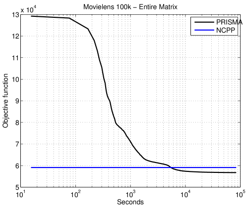
To demonstrate the applicability of PRISMA, we conducted runtime experiments on the MovieLens 100K Dataset444http://www.grouplens.org/node/73, selecting an equal and increasing number of users and movies with the most ratings. We used training data equal to 25% of the total number of entries, selected uniformly at random among the ranked entries. We implemented PRISMA in MATLAB. We stopped PRISMA when the relative difference was less than . The computation bottleneck of the algorithm is the computation of the eigenvalue decomposition at each step. So, to speed-up the algorithm, we implemented the strategy to calculate only the top eigenvalues, where is defined as . If the smallest calculated eigenvalue is positive, we increase by 5 and recalculate them, otherwise we proceed with the projection step. This strategy is based on the empirical observation that the algorithm produces solutions of decreasing rank, and practically this procedure gives a big speed-up to the algorithm. This kind of strategy is common in the matrix completion literature and RPCA, see e.g. Goldfarb et al. (2009). We compared our algorithm to SDPT3 Tütüncü et al. (2003), a state-of-the package for semidefinite-quadratic-linear programming. For simplicity the parameter was set the same in all the experiments, equal to that guarantees reasonable good generalization performance for all the sizes considered. The parameter of PRISMA was set to a rough estimate of the optimal value, that is, to . The running times and the final value of the objective function are listed in Table 1. SDPT3, a highly optimized SDP solver relying on interior point methods, indeed has very good performance for relatively small problems. But very quickly, the poor scaling of interior point methods kick in, and the runtime increases dramatically. More importantly, SDPT3 ran out of memory and could not run on problems of size 300x300 or larger, as did other SDP solvers we tried. On the other hand, the number of iterations required by PRISMA to reach the required precision increases only mildly with the size of the matrices and the increase in time is mainly due to the more expensive SVDs. We could run PRISMA on much larger problems, including the full MovieLens 100K data set. In Figure 1 we report the objective value as function of time (in seconds) for PRISMA on this data set. The time of each PRISMA iteration decreased over time, as the rank of the iterate decreases, ranging from 30 seconds of the first iterations to 2 seconds of the last ones, yielding a total runtime of several hours on the entire dataset. In contrast, it is inconceivable to use generic SDP methods for such data. On the other extreme, non-convex proximal-point (NCPP) methods are indeed much faster on this (and even much larger) data sets, taking only about ten seconds to reach a reasonable solution. However, even running NCPP for many hours with different step size settings and regardless of the allowed dimensionality, NCPP was not able to reach the global minimum, and was always at least worst than the solution found by PRISMA—the minimum objective value attained by NCPP is also plotted in Figure 1. PRISMA thus fills a gap between the very pricey SDP methods that are practical only on tiny data sets, and the large-scale NCPP methods which require significant parameter tweaking and produce only rough (even if sometimes satisfying) solutions.
| SDPT3 | PRISMA | ||||
|---|---|---|---|---|---|
| Matrix Size | Cost | Time | Cost | Iter. | Time |
| 100x100 | 1078.76 | 13s | 1079.00 | 7366 | 124s |
| 150x150 | 2617.65 | 89s | 2618.11 | 7866 | 218s |
| 200x200 | 4795.76 | 364s | 4796.97 | 8908 | 281s |
| 250x250 | 7736.76 | 1323s | 7738.59 | 9524 | 404s |
| 300x300 | – | – | 11406.39 | 9843 | 578s |
4.2 Robust PCA
In the method of Candes et al. (2011) for robust PCA, a data matrix is given and the goal is to solve
| (4.2) |
This problem is of the form (1.1) with the choice . We used the RPCA method to solve the task of background extraction from surveillance video. By stacking the columns of each frame into a long vector, we get a matrix whose columns correspond to the sequence of frames of the video. This matrix can be decomposed into the sum of two matrices . The matrix , which represents the background in the frames, should be of low rank due to the correlation between frames. The matrix , which represents the moving objects in the foreground in the frames, should be sparse since these objects usually occupy a small portion of each frame.
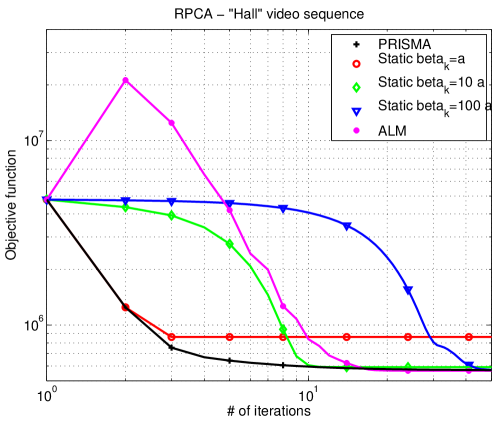
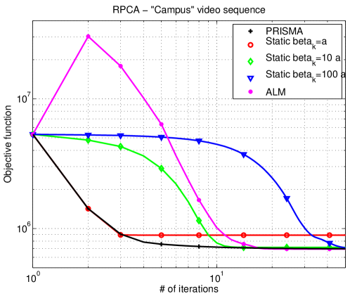
We have compared our MATLAB implementation of PRISMA to ALM Goldfarb et al. (2009, 2012), where this problem is solved with an augmented Lagrangian method, smoothing both the trace and the norm. We further used the ALM continuation strategy described in Goldfarb et al. (2009), that is usually beneficial in practice even though no theoretical iteration count guarantees are known for it. The parameter of PRISMA, analogously to max-norm experiments, is set to . We also compared it to the static strategy, setting to constant times .
In our experiments, we used two videos555http://perception.i2r.a-star.edu.sg/bk_model/bk_index.html introduced in Li et al. (2004), “Hall” and ”Campus” with the same parameters used in Goldfarb et al. (2009). Since for all algorithms the complexity for each update is roughly the same, and dominated by an SVD computation, we directly compare the number of iterations in order to reduce the hardware/implementation dependence of the experiments. The average CPU time per iteration for the algorithms and datasets are reported in Table 2. The results are shown in Figure 2. On both image sequences PRISMA outperforms the static algorithm, uniformly over the number of iterations. Notice also that for some constant settings the algorithm does not converge to the optimum, as expected from Theorem 3.1. Moreover it also outperforms the state-of-the-art algorithm ALM.
| Campus | Hall | |
|---|---|---|
| PRISMA (static & dynamic) | ||
| ALM |
4.3 Sparse Inverse Covariance Selection
In sparse inverse covariance selection (SICS) – see Wainwright et al. (2007); Yuan and Lin (2007) and references therein – the goal is to solve
| (4.3) |
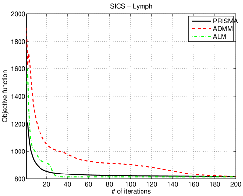
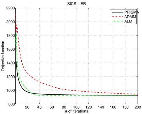
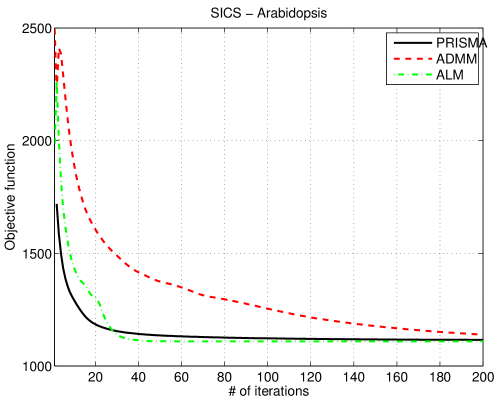
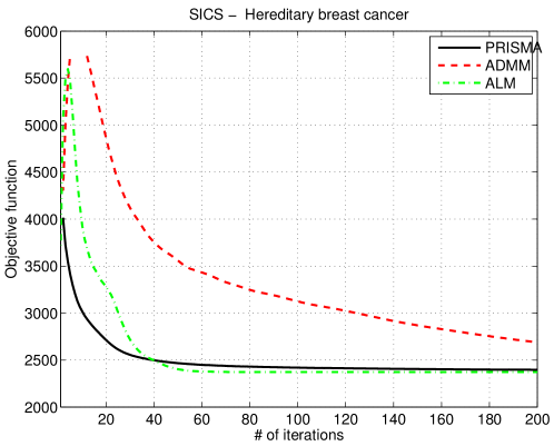
where is a given positive semidefinite matrix. This problem is of the form (1.1) with the choice , . The required proximity operator of at can be easily computed by computing a singular value decomposition of and solving a simple quadratic equation to obtain each singular value of the result. We have compared PRISMA with two state-of-the-art approaches: ALM Scheinberg et al. (2010), which achieves stats-of-the-art empirical results, and ADMM Boyd et al. (2011)666We used the MATLAB code available at http://www.stanford.edu/~boyd/papers/admm/., a recently popular general optimization method that performs very well in practice, but lacks iteration complexity guarantees.
ALM uses a complex continuation strategy that requires tuning of four different parameters – we used the data-set specific parameter settings provided by Scheinberg et al. (2010). For ADMM we used the default parameters. For both ALM and ADMM there is no clear theory on how to set their parameters. To set the parameter of PRISMA we need a rough estimate of . The optimal solution of (4.3) will be very close to a diagonal matrix, so we approximate its optimum of adding the constraint , and it is easy to see that the optimal is . Using the fact that , we set in all experiments. That is, both for ADMM and PRISMA we did not specifically tune any parameters.
We experimented on same five gene expression network data sets from Li and Toh (2010), which were also used by Scheinberg et al. (2010), and used the same setting .
The results on the datasets are shown in Fig. 3-7. Again we show the objective function in relation to the number of iterations, being the complexity per step of the algorithms roughly the same. The average times per iteration are reported in Table 3,4. We can see that the performance of PRISMA is pretty close to the one of ALM, while ADMM results in a slower convergence. Notice that the difference between ALM and ADMM is probably mainly due to the continuation strategy used in ALM, whose parameters are been tuned on these datasets. On the other hand PRISMA just has one parameter, whose optimal setting is given by the theory.
| Hereditary breast cancer | Lymph | |
|---|---|---|
| PRISMA | ||
| ALM | ||
| ADMM |
| Estrogen receptor | Arabidopsis thaliana | Leukemia | |
|---|---|---|---|
| PRISMA | |||
| ALM | |||
| ADMM |
5 Discussion and Future work
We have proposed PRISMA, a new algorithm which can be used to solve many convex nonsmooth optimization problems in machine learning, signal processing and other areas. PRISMA belongs to the broad family of proximal splitting methods and extends in different ways forward-backward splitting, accelerated proximal, smoothing and excessive gap methods. PRISMA is distinguished from these methods by its much wider applicability, which allows for solving problems such as basis pursuit or semidefinite programs such as max norm matrix completion.
We have validated our method with experiments on matrix completion, robust PCA problems, and sparse inverse covariance selection, showing that a simple to code implementation of PRISMA can handle large scale problems and outperforms or be equal in efficiency to current state of the art optimization algorithms. But PRISMA can be useful also for other learning-related problems.
For example, Basis Pursuit (BP) Chen et al. (2001); Guigue et al. (2005) can also be solved with PRISMA. The BP optimization problem is formulated as
| (5.1) |
where are prescribed input/output data. In most applications, the sample size is much smaller than the dimensionality, . This problem is of the form (1.1) with the choice , where . BP can be rephrased as a linear program, which is then solved with standard approaches (simplex, interior point methods, etc.), or it can be solved with ADMM, but in both cases no complexity results are known. It is easy to see that, for every , its projection on can be written as , where is any solution of , hence we can use PRISMA to solve this problem. The complexity of the projection step is , since . It would be interesting to see whether PRISMA would indeed yield empirical advantages here, as well as in varied other learning and optimization problems.
References
- Bauschke and Combettes [2011] H. H. Bauschke and P. L. Combettes. Convex Analysis and Monotone Operator Theory in Hilbert Spaces. CMS Books in Mathematics. Springer, 2011.
- Beck and Teboulle [2009] A. Beck and M. Teboulle. A fast iterative shrinkage-thresholding algorithm for linear inverse problems. SIAM Journal of Imaging Sciences, 2(1):183–202, 2009.
- Boyd et al. [2011] S. Boyd, N. Parikh, E. Chu, B. Peleato, and J. Eckstein. Distributed optimization and statistical learning via the alternating direction method of multipliers. Foundations and Trends in Machine Learning, 3(1):1–122, 2011.
- Cai et al. [2008] J. F. Cai, E. J. Candes, and Z. Shen. A singular value thresholding algorithm for matrix completion. SIAM Journal on Optimization, 20(4):1956–1982, 2008.
- Candes et al. [2011] E. J. Candes, X Li, Y. Ma, and J. Wright. Robust principal component analysis? Journal of the Association for Computing Machinery, 58(3), 2011.
- Chambolle and Pock [2011] A. Chambolle and T. Pock. A first-order primal-dual algorithm for convex problems with applications to imaging. Journal of Mathematical Imaging and Vision, 40(1):120–145, 2011.
- Chen et al. [2001] S. S. Chen, D. L. Donoho, and M. A. Saunders. Atomic decomposition by basis pursuit. SIAM Review, 43(1):129–159, 2001.
- Duchi and Singer [2009] J. Duchi and Y. Singer. Efficient online and batch learning using forward backward splitting. The Journal of Machine Learning Research, 10:2899–2934, 2009.
- Foygel and Srebro [2011] R. Foygel and N. Srebro. Concentration-based guarantees for low-rank matrix reconstruction. 24th Annual Conference on Learning Theory (COLT), 2011.
- Goldfarb et al. [2009] D. Goldfarb, S. Ma, and K. Scheinberg. Fast alternating linearization methods for minimizing the sum of two convex functions. arXiv:0912.4571, 2009.
- Goldfarb et al. [2012] D. Goldfarb, S. Ma, and K. Scheinberg. Fast alternating linearization methods for minimizing the sum of two convex functions. Mathematical Programming, pages 1–34, 2012.
- Guigue et al. [2005] V. Guigue, A. Rakotomamonjy, and S. Canu. Kernel basis pursuit. In Proceedings of the Sixteenth European Conference on Machine Learning, pages 146–157. Springer, 2005.
- Jaggi [2011] M. Jaggi. Convex optimization without projection steps. arXiv:1108.1170, 2011.
- Jaggi and Sulovsky [2010] M. Jaggi and M. Sulovsky. A simple algorithm for nuclear norm regularized problems. In Proceedings of the 27th International Conference on Machine Learning (ICML 2010), pages 471–478, 2010.
- Jalali and Srebro [2012] A. Jalali and N. Srebro. Clustering using max-norm constrained optimization. In International Conference on Machine Learning, 2012.
- Lee et al. [2010] J. Lee, B. Recht, R. Salakhutdinov, N. Srebro, and J. Tropp. Practical large-scale optimization for max-norm regularization. In Advances in Neural Information Processing Systems 23, pages 1297–1305, 2010.
- Li and Toh [2010] L. Li and K.-C. Toh. An inexact interior point method for l1-regularized sparse covariance selection. 2010.
- Li et al. [2004] L Li, W Huang, I Y Gu, and Q Tian. Statistical modeling of complex backgrounds for foreground object detection. IEEE Trans Image Process, 13(11):1459–1472, 2004.
- Loris and Verhoeven [2011] I. Loris and C. Verhoeven. On a generalization of the iterative soft-thresholding algorithm for the case of non-separable penalty. Inverse Problems, 27(12):125007, 2011.
- Ma et al. [2009] S. Ma, D. Goldfarb, and L. Chen. Fixed point and Bregman iterative methods for matrix rank minimization. Mathematical Programming, pages 1–33, 2009.
- Nesterov [2004] Y. Nesterov. Introductory lectures on convex optimization: A basic course. Springer, 2004.
- Nesterov [2005a] Y. Nesterov. Excessive gap technique in nonsmooth convex minimization. SIAM J. on Optimization, 16(1):235–249, May 2005a.
- Nesterov [2005b] Y. Nesterov. Smooth minimization of non-smooth functions. Mathematical Programming, 103(1):127–152, 2005b.
- Ouyang and Gray [2012a] H. Ouyang and A. Gray. Stochastic smoothing for nonsmooth minimizations: Accelerating SGD by exploiting structure. In Proceedings of the 29th International Conference on Machine Learning (ICML 2012), 2012a.
- Ouyang and Gray [2012b] H. Ouyang and A. Gray. Stochastic smoothing for nonsmooth minimizations: Accelerating SGD by exploiting structure. arXiv:1205.4481, 2012b.
- Scheinberg et al. [2010] K. Scheinberg, S. Ma, and D. Goldfarb. Sparse inverse covariance selection via alternating linearization methods. In Advances in Neural Information Processing Systems 23, pages 2101–2109. 2010.
- Shalev-Shwartz et al. [2010] S. Shalev-Shwartz, N. Srebro, and T. Zhang. Trading accuracy for sparsity in optimization problems with sparsity constraints. SIAM Journal on Optimization, 20(6), 2010.
- Srebro et al. [2005] N. Srebro, J. D. M. Rennie, and T. S. Jaakkola. Maximum-margin matrix factorization. In Advances in Neural Information Processing Systems 17, pages 1329–1336. MIT Press, 2005.
- Tomioka et al. [2010] R. Tomioka, T. Suzuki, M. Sugiyama, and H. Kashima. A fast augmented Lagrangian algorithm for learning low-rank matrices. In International Conference on Machine Learning, 2010.
- Tütüncü et al. [2003] Reha H. Tütüncü, K. C. Toh, and Michael J. Todd. Solving semidefinite-quadratic-linear programs using sdpt3. Math. Program., 95(2):189–217, 2003.
- Wainwright et al. [2007] M. J. Wainwright, P. Ravikumar, and J. D. Lafferty. High-dimensional graphical model selection using -regularized logistic regression. In Advances in Neural Information Processing Systems 19, pages 1465–1472, 2007.
- Yuan and Lin [2007] M. Yuan and Y. Lin. Model selection and estimation in the Gaussian graphical model. Biometrika, 94(1):19–35, 2007.