Calculating Dispersion Interactions using Maximally Localised Wannier Functions

Abstract

We investigate a recently developed approachSilvestrelli (2008, 2009a) that uses maximally-localized Wannier functions (MLWFs) to evaluate the van der Waals (vdW) contribution to the total energy of a system calculated with density-functional theory (DFT). We test it on a set of atomic and molecular dimers of increasing complexity (argon, methane, ethene, benzene, phthalocyanine, and copper phthalocyanine) and demonstrate that the method, as originally proposed, has a number of shortcomings that hamper its predictive power. In order to overcome these problems, we have developed and implemented a number of improvements to the method and show that these modifications give rise to calculated binding energies and equilibrium geometries that are in closer agreement to results of quantum-chemical coupled-cluster calculations.

Published as J. Chem. Phys. 135, 154105 (2011).

I Introduction

Local and semi-local exchange-correlation functionals used in density-functional theory Hohenberg and Kohn (1964); Kohn and Sham (1965) (DFT) can not account for the effect of long-ranged dispersion, or van der Waals (vdW), interactions. Dispersion interactions are crucial for weakly-bound systems, particularly where no covalent or ionic bonding is present, and often dominate intermolecular binding energies and equilibrium geometries. Incorporating vdW interactions in DFT remains a challenging task and a wide variety of methods have been developed, approaching the problem from many different perspectives Zaremba and Kohn (1976); Lundqvist et al. (1995); Andersson, Langreth, and Lundqvist (1996); Dobson and Dinte (1996); Kohn, Meir, and Makarov (1998); Dobson and Wang (1999); Rydberg et al. (2000); Dion et al. (2004); Tkatchenko and Scheffler (2009). In this work we focus on the method recently proposed by Silvestrelli Silvestrelli (2008, 2009a), which has been recently applied to various systems Silvestrelli (2009b); Silvestrelli, Toigo, and Ancilotto (2009); Costanzo et al. (2010); Silvestrelli et al. (2009) and implemented in a number of modern electronic structure codes Giannozzi et al. (2009); Gonze et al. (2009). This approach uses maximally-localized Wannier functions Marzari and Vanderbilt (1997) (MLWFs) as a means of decomposing the electronic density of the system into a set of localized but overlapping fragments, which may then be used to calculate a vdW correction to the DFT total energy by considering pairwise interactions between density fragments as derived by Andersson, Langreth and Lundqvist Andersson, Langreth, and Lundqvist (1996) (ALL).

In this Article, we explore the parameters and approximations involved in Silvestrelli’s method and improve its results where possible by modifying various aspects of the method. We apply the method and our proposed modifications to a series of test systems, then to two more challenging systems, a phthalocyanine and a copper phthalocyanine dimer. We thus demonstrate that although this method can offer an easily implementable and computationally efficient way of calculating the dispersion correction to the energy with the possibility of improved accuracy (once some modifications are applied to it), it is largely dependent on a number of parameters and choices one can make.

The remainder of the Article is organized as follows: in Sec. II we recap the necessary background theory relating to MLWFs and Silvestrelli’s method; in Sec. III we highlight some of the problems with the method as it stands, and describe our improvements; in Sec. IV we then present and discuss results for vdW-corrected total energies and equilibrium geometries obtained by applying these methods to a series of dimer systems and compare to quantum chemical coupled-cluster and semi-empirical vdW (DFT+D) approaches; finally, in Sec. V we draw our conclusions.

II Theoretical Background

II.1 Maximally-Localized Wannier Functions

Wannier functions Wannier (1937) are orthogonal localized functions that span the same space as the eigenstates of a single particle Hamiltonian. Consider the set of $N_{{\rm occ}}$ occupied (valence) eigenstates $\{|u_{m}\rangle\}$ of a molecule. The total energy is invariant with respect to unitary transformations among the eigenstates

$$|{w_{n}}\rangle=\sum_{m=1}^{N_{{\rm occ}}}U_{mn}|{u_{m}}\rangle.$$ (1)

If the unitary matrix $\mathbf{U}$ is chosen such that the resulting $N_{{\rm occ}}$ orbitals $\{w_{n}({\bf r})\}$ minimize their total quadratic spread, given by

$$\Omega=\sum_{n}\left(\langle w_{n}|r^{2}|w_{n}\rangle-\langle w_{n}|{\bf r}|w_{n}\rangle^{2}\right)=\sum_{n}\left(\langle r^{2}\rangle_{n}-\bar{{\bf r}}_{n}^{2}\right),$$ (2)

then they are said to be maximally-localized Wannier functions Marzari and Vanderbilt (1997) (MLWFs). Each MLWF is characterized by a value for its quadratic spread, $S_{n}^{2}$, and its centre, $\bar{{\bf r}}_{n}$.

In the construction of MLWFs it is sometimes useful to consider not only the valence manifold but also a range of unoccupied eigenstates above the Fermi level — often those constituting the antibonding counterparts to the valence states. This not only allows the MLWFs to be more localized Thygesen, Hansen, and Jacobsen (2005a, b) but can also restore symmetries that would otherwise be broken arbitrarily through the construction of MLWFs for the valence manifold only.

In order to do so, one defines an outer energy window, $E_{{\rm win}}$, consisting of $N_{{\rm win}}\geq N_{{\rm occ}}$ states, from which one may extract an optimal $N_{{\rm dis}}$-dimensional subspace ($N_{{\rm win}}\geq N_{{\rm dis}}\geq N_{{\rm occ}}$) using the disentanglement approach described in Ref. Souza, Marzari, and Vanderbilt, 2001,

$$|{u_{m}^{{\rm opt}}}\rangle=\sum_{p=1}^{N_{{\rm win}}}U_{pm}^{{\rm dis}}|{u_{p}}\rangle,$$ (3)

where $\mathbf{U}^{{\rm dis}}$ is a rectangular $N_{{\rm win}}\times N_{{\rm dis}}$ unitary matrix. $N_{{\rm dis}}$ MLWFs may then be localized by suitable rotation of the optimal subspace in the usual manner:

$$|{w_{n}^{{\rm dis}}}\rangle=\sum_{m=1}^{N_{{\rm dis}}}U_{mn}|{u_{m}^{{\rm opt}}}\rangle.$$ (4)

or, in terms of the Bloch states:

$$|{w_{n}^{{\rm dis}}}\rangle=\sum_{m=1}^{N_{{\rm dis}}}\sum_{p=1}^{N_{{\rm win}}}U_{mn}U_{pm}^{{\rm dis}}|{u_{p}}\rangle.$$ (5)

Furthermore, an inner, or frozen, energy window may be defined if one wishes to make certain that a range of low-lying eigenstates are included in the optimal subspace, for example, the occupied states. Algorithms for determining MLWFs from the eigenstates obtained from electronic structure calculations are implemented within the Wannier90 software package Mostofi et al. (2008).

The single-particle density operator is given by

$$\hat{\rho}=\sum_{1}^{N_{{\rm occ}}}|{u_{n}}\rangle\langle{u_{n}}|.$$ (6)

It can also be written in terms of the $N_{{\rm occ}}$ fully-occupied valence MLWFs, $|{w_{n}}\rangle$ or equivalently in terms of a larger set of $N_{{\rm dis}}$ disentangled MLWFs $|{w_{n}^{{\rm dis}}}\rangle$ that span the occupied subspace, which can be guaranteed by using a suitable frozen/inner window in the disentanglement procedure, and that have occupancies $f_{kl}^{w}$,

$$\hat{\rho} =\sum_{n=1}^{N_{{\rm occ}}}|{w_{n}}\rangle\langle{w_{n}}|,$$ (7)

$$=\sum_{k,l=1}^{N_{{\rm dis}}}f_{kl}^{w}|{w_{k}^{{\rm dis}}}\rangle\langle{w_{l}^{{\rm dis}}}|,$$ (8)

where we have substituted Eq. (1) and Eq. (5), respectively, into Eq. (6), and where the occupancies are given by

$$f_{kl}^{w}=\sum_{p=1}^{N_{{\rm occ}}}\sum_{m,s=1}^{N_{{\rm dis}}}U_{ml}U_{pm}^{{\rm dis}}U_{sk}^{*}U_{ps}^{*{\rm dis}}.$$ (9)

We can write the density as a sum of diagonal ($l=k$) and off-diagonal ($l\neq k$) terms,

$$\rho({\bf r}) =\sum_{l=1}^{N_{{\rm dis}}}f_{ll}^{w}|w_{l}^{{\rm dis}}({\bf r})|^{2}+\sum_{l\neq m}^{N_{{\rm dis}}}f_{lm}^{w}w_{l}^{*{\rm dis}}({\bf r})w_{m}^{{\rm dis}}({\bf r}),$$

$$\equiv\rho_{D}({\bf r})+\rho_{OD}({\bf r}).$$ (10)

It is important to note that in this form, $\rho_{D}({\bf r})$ alone integrates to the number of valence electrons $N_{e}$, because the mututal orthogonality of the MLWFs ensures $\int\rho_{\rm OD}({\bf r})d{\bf r}=0$.

In the case of considering MLWFs obtained from the manifold of occupied states only ($N_{\rm dis}=N_{\rm occ}$), the the occupancy matrix is simply the identity matrix, $f_{kl}=\delta_{kl}$, and the charge density in terms of the MLWFs is simply given by

$$\rho({\bf r})=\sum_{n=1}^{N_{\rm occ}}|w_{n}({\bf r})|^{2}$$ (11)

It is worth noting that in the case of spin-degenerate systems, the occupancies must be scaled by a factor of 2.

We have adapted the Wannier90 code to calculate the occupation matrices, and can choose to make a diagonal approximation to the density by retaining only the first term of Eq. (10). The effect of approximating the true density with the diagonal approximation will be discussed later in Sec. IV.9 in the context of the improvements, described in Sec. III, to Silvestrelli’s method.

II.2 Silvestrelli’s method

Silvestrelli’s approach Silvestrelli (2008, 2009a) is based on the Andersson, Langreth and Lundqvist Andersson, Langreth, and Lundqvist (1996) (ALL) expression for the vdW energy in terms of pairwise interactions between density fragments $\rho_{n}({\bf r})$ and $\rho_{l}({\bf r}^{\prime})$, separated by a distance $r_{nl}$,

$$E_{{\rm vdW}}=-\sum_{n>l}g_{nl}(r_{nl})\frac{C_{6nl}}{{r_{nl}^{6}}},$$ (12)

where $g_{nl}(r_{nl})$ is a damping functionSilvestrelli (2009a) which screens the unphysical divergence of Eq. (12) at short range, and

$$C_{6nl}=\frac{3}{4(4\pi)^{3/2}}\int_{V}d{\bf r}\int_{V^{\prime}}d{\bf r}^{\prime}\frac{\sqrt{\rho_{n}({\bf r})\rho_{l}({\bf r}^{\prime})}}{\sqrt{\rho_{n}({\bf r})}+\sqrt{\rho_{l}({\bf r}^{\prime})}},$$ (13)

in atomic units. It should be noted that these expressions are only strictly valid in the limit of non-overlapping density fragments. There are various forms for the damping functionGrimme et al. (2007); Wu et al. (2001) that might have a slight short-range effect but should not affect the long-range behaviour of the vdW energies. Here we chose to use the damping function as proposed in the original paper by SilvestrelliSilvestrelli (2008).

Now, in accord with Eq. (11), the MLWFs obtained from the valence orbitals of a system provide a localized decomposition of the electronic charge density, such that $\rho_{n}({\bf r})=|w_{n}({\bf r})|^{2}$, so that Eq. (13) becomes

$$C_{6nl}=\frac{3}{32\pi^{3/2}}\int_{|{\bf r}|\leq r_{c}}d{\bf r}\int_{|{\bf r}^{\prime}|\leq r_{c}^{\prime}}d{\bf r}^{\prime}\frac{|w_{n}({\bf r})||w_{l}({\bf r}^{\prime})|}{|w_{n}({\bf r})|+|w_{l}({\bf r}^{\prime})|},$$ (14)

where $r_{c}$ is a suitably chosen cutoff radius obtained by equating the length scale for density change to the electron gas screening length Silvestrelli (2009a); we will revisit this point later.

In order to make the calculation of the integrals more tractable, the charge density is approximated by replacing each MLWF $w_{n}(\mathbf{r})$ with a hydrogenic $s$-orbital that has the same centre $\bar{{\bf r}}_{n}$ and spread $S_{n}$ as the MLWF, and whose analytic form is is given by

$$w^{H}_{n}({\bf r})=\frac{3^{3/4}}{\sqrt{\pi}S_{n}^{3/2}}e^{-\sqrt{3}|\mathbf{r}-\bar{{\bf r}}_{n}|/S_{n}},$$ (15)

which, on substitution into Eq. (14) and after some algebra, gives

$$C_{6nl}=\frac{S_{n}^{3/2}S_{l}^{3}}{2\cdot 3^{5/4}}F(S_{n},S_{l}),$$ (16)

where

$$F(S_{n},S_{l})=\int_{0}^{x_{c}}dx\int_{0}^{y_{c}}dy\frac{x^{2}y^{2}e^{-x}e^{-y}}{e^{-x}/\beta+e^{-y}},$$ (17)

$\beta=(S_{n}/S_{l})^{3/2}$, $x_{c}=\sqrt{3}r_{c}/S_{n}$ and $y_{c}=\sqrt{3}r_{c}^{\prime}/S_{l}$. Whereas evaluating Eq. (14) using the true MLWFs requires a computationally demanding six-dimensional numerical integration, Eq. (17) may be evaluated easily since it is only a two-dimensional integral that depends solely on the MLWF spreads and centres, not their detailed shapes or orientations.

We note that in the case of a spin-degenerate system, since every MLWF is doubly occupied, the density of each fragment must be multiplied by a factor of 2 and, therefore, the $C_{6nl}$ integral in Eq. (14) must be scaled by a factor of $\sqrt{2}$.

III Improvements to Silvestrelli’s Method

The approximations that go into the method described in the previous Section will clearly not always hold, and the need to examine them is clear. In this Section, we introduce our enhancements to the method that address possible drawbacks.

III.1 Partly Occupied Wannier Functions

Using a manifold of eigenstates that includes but is larger than the subspace spanned by just the valence states results in partly-occupied MLWFs that are generally more localized and that better reflect the symmetries of the system, as opposed to MLWFs obtained by rotation of the valence subspace only, which arbitrarily break the symmetry (we will demonstrate examples of this phenomenon in Sec. IV).

In order to account for the partial occupancy of the MLWFs, we make a slight modification to Silvestrelli’s approach, explicitly introducing occupancies in the definition of the $C_{6nl}$ integral; since in the diagonal approximation, the density of each fragment is now given by $\rho_{n}({\bf r})=f_{nn}^{w}|w_{n}({\bf r})|^{2}$, the expression for $F(S_{n},S_{l})$ in Eq. (17) becomes

$$F(S_{n},S_{l})=\int_{0}^{x_{c}}dx\int_{0}^{y_{c}}dy\frac{x^{2}y^{2}e^{-x}e^{-y}}{e^{-x}/(\beta\sqrt{f_{nn}^{w}})+e^{-y}/\sqrt{f_{ll}^{w}}},$$ (18)

where the $f_{nn}^{w}$ are given by Eq. (9). We will see in Sec. IV that this seemingly simple idea can give rise to a marked improvement in the accuracy of the method.

III.2 Modification to describe $p$-like states

MLWFs describing only the valence manifold often take the form of well-localized functions centred on a bond between two atoms, and are thus reasonably well-described by the approximation of replacing them with a suitable $s$-orbital. When anti-bonding states are included in the construction of the MLWFs, the resulting orbitals have more atomic-orbital character. This is demonstrated by the atom-centred $p$-like MLWF shown in Fig. 1. It is clear that the density associated with such an MLWF will not be very well represented by a single $s$-like function at its centre. In order to approximate $p$-like orbitals appropriately when calculating $C_{6}$, one could imagine using a suitably-oriented analytic expression for a hydrogenic $p$-orbital, for example, a canonical $p_{z}$-orbital given by

$$p_{z}({\bf r})=\frac{30^{5/4}r\cos{\theta}}{\sqrt{32\pi}S^{5/2}}e^{-\sqrt{30}r/2S},$$ (19)

which has been normalized such that its quadratic spread is $\langle p_{z}|({\bf r}-\bar{{\bf r}})^{2}|p_{z}\rangle=S^{2}$. As a consequence of the explicit angular dependence, using this function in Eq. (14) would give rise to four-dimensional integrals for which analytic solutions are not readily available. Numerical evaluation of these integrals, for realistic systems, would be prohibitively computationally expensive. We solve this problem by identifying the $p$-like MLWFs in the system and replacing them with the hydrogenic form given in Eq. (19). Then, we further approximate each lobe (lower and upper) of this $p$-like orbital with two separate hydrogenic $s$-orbitals of the form of Eq. (15). In order to do so, for each of the upper ($+$) and lower ($-$) lobes of the orbital, it is necessary to know the spread $S_{\pm}$ and centre $\bar{{\bf r}}_{\pm}$, given by

$$S_{\pm}^{2} =\int_{0}^{\infty}\int_{0}^{\pi/2}\int_{0}^{2\pi}r^{4}p_{z}^{2}({\bf r})\sin\theta drd\theta d\phi,$$ (20)

$$\bar{{\bf r}}_{\pm} =\bar{{\bf r}}\hskip 2.84526pt\pm\int_{0}^{\infty}\int_{0}^{\pi/2}\int_{0}^{2\pi}r^{3}\cos\theta\,p_{z}^{2}({\bf r})\sin\theta drd\theta d\phi\>\hat{{\bf z}},$$ (21)

which, after some algebra, simplifies to

$$S_{\pm} =\frac{7S}{8\sqrt{2}},$$ (22)

$$\bar{{\bf r}}_{\pm} =\bar{{\bf r}}{}\pm\frac{15S}{8\sqrt{30}}\>\hat{{\bf z}},$$ (23)

where $\bar{{\bf r}}$ and $S$ are the original centre and spread, respectively, of the true MLWF. These expressions may be easily generalized to arbitrary orientations of the symmetry axis of a $p$-like state by rotating the offset vectors $(\bar{{\bf r}}_{\pm}-\bar{{\bf r}})$ accordingly.

Thus, we have developed a formalism whereby the charge density due to MLWFs with $p$-like character can be represented by a pair of $s$-like hydrogenic orbitals with appropriate centres and spreads. In Sec. IV we will show how this works in practice for calculating vdW energy corrections.

In the relatively simple systems studied in this paper, the $p$-like orbitals are easily distinguished from other orbitals by their partial occupancies, given by Eq. (9), which are typically closer to 0.5 rather than 1. Alternatively, and especially for structurally more complex systems, the shape of each MLWF could be characterized using the efficient method described in Appendix A of Ref. Shelley et al., 2011 as another means of automating the procedure of identifying $p$-like functions.

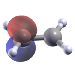
Figure 1: Partly occupied $p$-like orbital on ethene molecule. In the method described here, each of the two lobes (coloured red and blue) is replaced by an $s$ orbital and considered a separate fragment.

III.3 Symmetry Considerations

Minimizing the total spread $\Omega$ with respect to the elements of the unitary matrix $\mathbf{U}$, and thus producing MLWFs, has the effect of picking from the space of all possible unitary matrices one which produces the most localized Wannier functions accessible through optimization from a chosen initial guess. This is often enough to uniquely determine the MLWFs. In some cases, however, it does not give rise to a unique choice, even if the optimization procedure is perfect. For example, the atomic positions and electron density of the system may possess certain symmetry elements, such as rotations about a particular axis. Then there will exist a number of equally valid and degenerate representations of the MLWFs and their centres, which give the same spread, and are related by symmetry. The minimization procedure breaks the symmetry by choosing one of these representations; in other words there will be a degree of arbitrariness in the final MLWFs. It is clear from Eq. (12) that any degree of non-uniqueness of the centres will cause an undesirable variability of the vdW energy calculated in Silvestrelli’s method. This is indeed what we observe in some of the examples below. Moving away from a description of the MLWFs using the valence states only, and towards using partly occupied MLWFs that include anti-bonding states and which retain the symmetries of the system, enables us to overcome these problems, as we demonstrate below.

IV Applications

IV.1 Calculation Details

For the application of Silvestrelli’s method to the following dimer systems we used the Quantum Espresso (QE) packageGiannozzi et al. (2009) to perform the ground-state DFT calculations, and Wannier90Mostofi et al. (2008) to obtain the centres and spreads of the MLWFs. Our results are compared to both the semi-empirical DFT+D methodGrimme (2006); Barone et al. (2009) as implemented in QE, which is expected to give good asymptotic behaviour, and a wavefunction-based coupled-cluster approach, CCSD(T), which is considered the ‘gold-standard’ of quantum chemistry.

The PBE Perdew, Burke, and Ernzerhof (1996) generalized-gradient approximation for exchange and correlation, except in the case of argon where the revPBE Zhang and Yang (1998) functional was used; norm-conserving pseudopotentials, and $\Gamma$-point sampling of the Brillouin zone were used throughout. We note that we have chosen to use revPBE for the argon system since PBE produces significant binding in rare gas dimers as it overestimates the long-range part of the exchange contributionDion et al. (2004, 2005); Chakarova-Käck et al. (2006). For all the other systems we studied in this manuscript, however, PBE does not cause spurious binding and would therefore normally be considered an appropriate functional. A plane-wave basis set cut-off energy of 80 Ry was used in all calculations with QE except for the case of the phthalocyanine and copper phthalocyanine where a 50 Ry energy cutoff was used. For the dimers of argon, methane, ethene, phthalocyanine and copper phthalocyanine, cubic simulation cells of length 15.87 Å, 15.87 Å, 21.16 Å and 23.81 Å, respectively, were used. For the dimers of benzene, a hexagonal cell with $a=15.87$ Å and $c=31.75$ Å was used. For all the systems, the choice of energy windows when using the disentanglement procedure in Wannier90 for our modified method was as follows: inner (frozen) energy windows were chosen to include all the valence states; outer energy windows ranged from the lowest eigenvalue of the system, $\epsilon_{0}$, to a maximum of $E_{{\rm win}}=\epsilon_{{\rm LUMO}}+\alpha(\epsilon_{{\rm HOMO}}-\epsilon_{0})$, where $\epsilon_{{\rm HOMO}}$ is the energy of the highest occupied valence Kohn-Sham (KS) state and $\epsilon_{{\rm LUMO}}$ is the energy of the lowest unoccupied KS state. The factor $\alpha=0.4$ was chosen to scale down the valence energy bandwidth, used to estimate the energy difference required above the LUMO when including anti-bonding states. We discuss the sensitivity of the method to this factor in Sec. IV.10.

IV.2 Argon

We will first investigate the severity of the aforementioned issues relating to symmetry, by considering the case of an argon dimer. Optimization of the MLWFs describing a single argon atom produces four doubly occupied MLWFs arranged tetrahedrally around the atom. Due to spherical symmetry, the orientation of these MLWFs with respect to a given coordinate system is arbitrary for an isolated atom and the final MLWFs obtained will depend on the initial guess used. In the dimer, this arbitrariness is removed, at least in principle, since the spherical symmetry is broken by the presence of the other atom at a specific orientation. At large separations, this is not in practice necessarily the case: the electron density overlap between the Ar atoms is vanishingly small, since the wavefunctions decay exponentially away from the atom. Therefore, to within attainable numerical precision, the orientation of the MLWFs on each atom is uncorrelated with the orientation of the other atom: the MLWFs can be freely rotated with respect to the atom without affecting the total spread. Note, however, that since the vdW energy only decays as $R^{-6}$, its value is influenced by the orientation of the MLWF centres (and hence their separation) out to distances beyond which the calculated spread (and thus the optimised MLWF orientation) has ceased to be sensitive to separation.

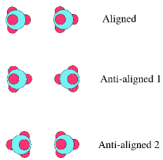
Figure 2: Illustration of three of the many possible configurations of MLWF centres (small pink spheres) for the two argon atoms (large blue spheres) in the fragment method.

This dependence can be investigated in a two-atom system by fixing the relative orientations of the MLWF centres between the two atoms in the dimer. This is achieved by first calculating the MLWF centres for a single atom of argon and then translating and rotating these centres to the second Ar atom with various choices of alignment. We will refer to this approach as the fragment method. In this method, we calculate the dispersion correction to the energy for a dimer system using various possible arrangements of MLWF centres on the other atom. Three possible high-symmetry choices are shown in Fig. 2. For each of these orientations, Fig. 3 (top) shows the binding energy of the Ar dimer as the separation of the atoms varies. We see that there is considerable displacement of the curves, and the binding energy and the equilibrium separation change according to the alignment chosen by up to $0.04$ kcal/mol and 0.08 Å, respectively.

In contrast to this fragment approach, in Fig. 3 (bottom) we show the binding energy as calculated with the normal approach of using the optimized MLWFs of the entire dimer system. However, here we have used varying initial guesses corresponding to the set of possible alignments shown in Fig. 2. We see that at small separations, the MLWF centres always converge to the same positions, regardless of the initial guess, and the binding energy curve is nearly independent of the choice of initial guess ($\sim 10^{-3}$ kcal/mol variation).

At larger separation, however, the spread minimization is insufficiently sensitive to the relative orientation of the MLWFs on different atoms, and does not necessarily alter it from the initial guess, resulting in several different possible results depending on the initial orientation of the centres. If a random initial guess is chosen, then the energy varies discontinuously, as a function of separation, within the bounds imposed by the limiting cases described using the fragment method. This is because the MLWF centres converge to different orientations depending on their starting positions (curve labelled ‘random’ in Fig. 3 (bottom)).

In order to avoid this problem of non-uniqueness of binding energy curves, a random initial guess is used first for a configuration at small separation, in the knowledge that the result will be independent of the guess used. Then the centres computed at the previous, smaller separation are used as the initial guess for the calculation at a larger separation. In this manner, a unique continuous curve is obtained (labelled ‘continuous’ in Fig. 3 (bottom)). This is the approach that we adopt for all subsequent calculations in this paper.

From the continuous curve, we obtain 3.97 Å for the equilibrium separation and $-0.28$ kcal/mol for the binding energy. This is in good agreement with the coupled cluster CCSD(T) calculations of Ref. Slavíc̆ek et al., 2003, which give 3.78 Å and $-0.28$ kcal/mol, respectively, whereas revPBE without dispersion corrections gives 4.62 Å and $-$0.04 kcal/mol.

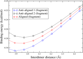
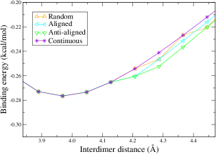
Figure 3: Binding energy versus interatomic separation for the argon dimer, for varying relative orientations of the MLWF centres surrounding each atom (see Fig. 2). Top panel: results obtained using the fragment method, in which the MLWF centres are calculated for a lone Ar atom and then translated and rotated to the second Ar atom. Bottom panel: results obtained using the true MLWF centres with various initial guesses for their positions. The curve labelled ‘continuous’ is obtained by using the MLWF centres from a configuration at small separation as the initial guess for the centres at larger separations. In this way, the discontinuities in the curve are avoided and a unique curve is obtained (see text for details).

IV.3 Methane

The methane dimer is a straightforward application of the Silvestrelli method: the positions of the MLWF centres, which lie on the four tetrahedral C-H bonds of each CH₄ molecule (see Fig. 4), obey the same symmetries as the atomic positions, so there exists no arbitrariness of orientation.

In Fig. 5, we compare to the results of both DFT+D and CCSD(T) calculations. Our geometries and CCSD(T) results were drawn from the Benchmark Energy and Geometry Database (BEGDB)R̆ezác̆ et al. (2008).

The accuracy of Silvestrelli’s method in the case of the methane dimer is good compared to CCSD(T): the former gives an equilibrium separation of 3.66 Å and binding energy of $-0.69$ kcal/mol, and the latter 3.72 Å and $-0.53$ kcal/mol, respectively. DFT+D is in somewhat worse agreement with CCSD(T), yielding 3.54 Å and $-0.76$ kcal/mol, respectively.

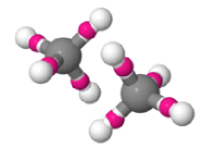
Figure 4: Illustration of the methane dimer. Carbon atoms are shown by large grey spheres, hydrogen by small white spheres, and the valence MLWF centres are shown by small pink spheres.

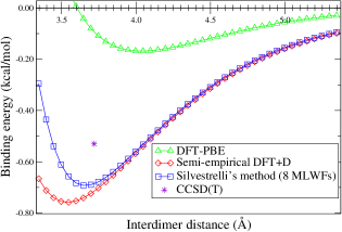
Figure 5: Binding energy curves for the methane dimer with various methods.

IV.4 Ethene

We now turn our attention to the ethene dimer, which includes a C-C double bond. Again we will compare results for the original and modified methods against CCSD(T) and DFT+D results. We have again used the geometries for each molecule taken from the BEGDB.

To use Silvestrelli’s original method in this case, we include only the valence manifold in the creation of the MLWFs, giving six MLWFs per molecule arranged as shown in Fig. 6 (left). In our modified method we use seven MLWFs per molecule, with $p$-like, partly occupied orbitals on each carbon atom (Fig. 6 (right)).

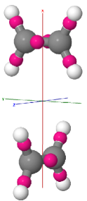
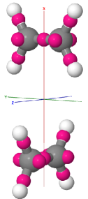
Figure 6: Colours as in Fig. 4. Left: Ethene dimer with six MLWFs per molecule. Right: Ethene dimer with seven MLWFs per molecule. The centres of the $p$-like MLWFs are placed on the carbon atoms, but here we show the centres of the individual lobes of these $p$-like orbitals as calculated by our method.

As seen in Fig. 7, neither the original Silvestrelli method (blue squares) nor DFT+D (red diamonds) reproduce the CCSD(T) values very accurately. By expanding the manifold of eigenstates used in the construction of the MLWFs and applying our modified method to include partial MLWF occupancies and splitting of the $p$-like functions (see Sec. III), we find an excellent agreement (black circles) with the CCSD(T) equilibrium values of 3.72 Å for the separation and $-1.51$ kcal/mol for the binding energy; our method gives 3.73 Å and $-1.60$ kcal/mol, respectively; Silvestrelli’s method gives 3.83 Å and $-1.69$ kcal/mol; DFT+D yields 3.55 Å and $-2.04$ kcal/mol.

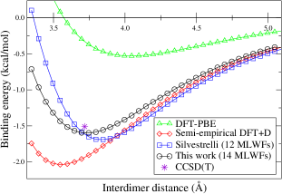
Figure 7: Binding energy for an ethene dimer with various methods.

IV.5 Benzene

For benzene, the valence states can be represented by 15 doubly-occupied Wannier functions. The MLWF optimization procedure in this case therefore breaks the $D_{6h}$ symmetry of the benzene ring: the end result is that there are three C-C ‘double’ bonds and three C-C ‘single’ bonds in the MLWF representation. Those alternating double and single C-C bonds represent a delocalised $\pi$-bond around the ring. The double bonds are represented by two centres located above and below the plane of the molecule, while the single bonds are represented by one centre on the bond. When two molecules are put in proximity (see Fig. 8) and the vdW energy is calculated by Silvestrelli’s method, the breaking of the symmetry affects the vdW energy in an arbitrary manner, dependent on how the two rings are aligned (i.e. whether the pairs of double bonds in adjacent molecules are aligned or anti-aligned). This alignment is defined by where the initial guesses for the centres of the Wannier functions are placed.

The case of the benzene dimer therefore illustrates again the need to include the unoccupied antibonding states in the construction of the MLWFs: doing so increases the number of MLWFs to 18 and introduces partial occupancies, but restores the $D_{6h}$ symmetry of the system and also localises the MLWFs more. This then makes the vdW contribution independent of the initial guess for the Wannier function centres.

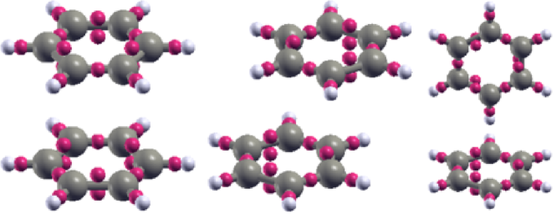
Figure 8: The three configurations used for the benzene dimer calculations: S (vertical displacement), PD (vertical and lateral displacement) and T (vertical displacement plus rotation in plane of one molecule), and the valence MLWF centres in each case (depicted by pink spheres).

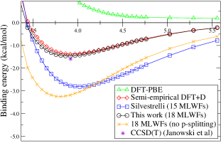
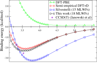
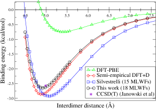
Figure 9: Binding energy (kcal/mol) curves for the various methods for the benzene dimer in the S, PD and T configurations (top, middle and bottom respectively). For the S configuration we also show the curve using 18 MLWFs per molecule if no $p$-splitting is used; in this case the method overbinds. CCSD(T) benchmark values are from Janowski et al. Janowski and Pulay (2007)

We applied our implementation of the original Silvestrelli’s method (with 15 MLWFs), and then our modified method (with 18 MLWFs, partial occupancies and splitting of $p$-like states) to determine the binding energy as a function of displacement for three types of displacement (labelled S, PD, and T, illustrated in Fig. 8 of one of the molecules in the benzene dimer. We compare this to DFT+D and to the CCSD(T) calculations of Ref. Janowski and Pulay, 2007. We note that we used the same bond lengths for C-C and C-H as Ref. Janowski and Pulay, 2007 to within two decimal places, to construct perfectly symmetric benzene rings for our calculations.

The binding energy curves for the various methods for the three configurations are shown in Fig. 9. Silvestrelli’s method (blue squares) does not agree very well with CCSD(T) calculations, overestimating equilibrium distances by 0.07-0.25 Å (Table 1) and overestimating binding energies by 0.28-1.25 kcal/mol (Table 2). In particular, the dispersion curve obtained from Silvestrelli’s method does not agree asymptotically with the DFT+D curve (red diamonds). In the T configuration Silvestrelli’s method performs better in terms of equilibrium distance, binding energy and asymptotics as it can be seen in Fig. 9 (bottom).

For the S configuration we also show the binding curve obtained if the anti-bonding states are included in the construction of the MLWFs, but splitting of the $p$-like states is not used (orange crosses); it is clear that in this case the method does not perform well, as replacing a $p$-like orbital by an $s$-orbital is a very poor approximation.

Our full modified method, including both the larger manifold and the splitting of $p$-like states (black circles in Fig. 9), on the other hand, has excellent agreement in terms of equilibrium distances and binding energies with the DFT+D curves and the CCSD(T) values, for all three configurations, to within 0.05 Å and 0.33 kcal/mol (Table 1 and 2); the asymptotic behaviour of the energy is also better captured.

Method	S	PD	T
Silvestrelli (15 MLWFs)	4.01	3.78	5.06
This work (18 MLWFs)	3.89	3.55	4.88
Semi-empirical DFT+D	3.93	3.58	4.89
CCSD(T) (Janowski et al Janowski and Pulay (2007))	3.92	3.53	4.99

Table 1: Equilibrium distances in Å for the benzene dimers in the three configurations (Fig. 8) using the various methods. For all DFT calculations the PBE functional was used.

Method	S	PD	T
Silvestrelli (15 MLWFs)	$-$2.85	$-$3.23	$-$2.85
This work (18 MLWFs)	$-$1.47	$-$2.31	$-$2.64
Semi-empirical DFT+D	$-$1.38	$-$2.11	$-$2.87
CCSD(T) (Janowski et al Janowski and Pulay (2007))	$-1.60$	$-2.55$	$-2.57$

Table 2: Binding energies (kcal/mol) at equilibrium geometry for the benzene dimers in the three configurations (Fig. 8) using the various methods. For all DFT calculations the PBE functional was used.

IV.6 H₂Pc and CuPc

To examine the difficulties encountered applying these methods to larger systems, we have investigated the phthalocyanine (H₂Pc) dimer in the simplest configuration (S vertically displaced) first by applying Silvestrelli’s method and then by applying our modifications it, and comparing the binding energy curve to one obtained using DFT+D. The optimised MLWF centres for a single H₂Pc are shown in Fig. 10 (top). We see that as with the benzene molecule, there are alternating single and double MWLF centres on the C-C bonds of the six-membered rings, representing delocalised $\pi$-bonds. We also find, however, that using only the 93 valence MLWFs (186 valence electrons) is problematic, as a good representation of the electronic density of the system cannot be obtained in this way since this breaks the symmetry of the system, but most importantly it yields one lone MLWF of unrealistically large spread ($\sim$2.5 Å) located some distance from any atoms (Fig. 10 (top)). This is due to the fact that an odd number (93 MLWFs) is incompatible with the $D_{2h}$ symmetry of the molecule.

Using a larger and even number of MLWFs (112 per molecule) we can restore this $D_{2h}$ symmetry of the molecule (Fig. 10 (bottom)) and represent the electronic density of the system in a way more compatible with its chemistry. When anti-bonding states are included, it is important to make a chemically intuitive initial guess for the centres and forms of the MLWFs. We make initial guesses as follows: we place $p$-like orbitals on the carbon atoms and $s$-like orbitals on every bond and $p$-like orbitals on the hydrogenated nitrogens as well as two $s$-like orbitals on every non-hydrogenated nitrogen atom. In this way, we have partly occupied MLWFs that represent the 372 valence electrons of the dimer. The binding energy curves obtained by using this representation and our modifications to Silvestrelli’s method are shown in Fig. 11 and compared to DFT+D. The binding energy obtained from our method is $-23.63$ kcal/mol and the equilibrium distance 3.58 Å; with DFT+D we obtain $-18.91$ kcal/mol and 3.68 Å. As for benzene, we see very good agreement with DFT+D; these values roughly agree with the stacking distance of crystalline H₂Pc (around 3.2–3.4 Å)Orti and Bredas (1988). Silvestrelli’s original method severely overbinds the dimer (giving a binding energy of $-41$ kcal/mol) because of the unphysically large spread of the lone MLWF that appears in the valence representation. This is due to the strong dependence of the vdW energy on the spreads (Eq. (16)).

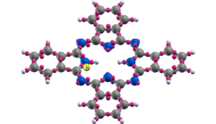
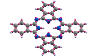
Figure 10: Left: Phthalocyanine ($\text{H}_{2}\text{Pc}$) molecule and its valence MLWF centres. Hydrogen atoms are by small white spheres, carbon atoms by large grey spheres and nitrogen atoms by large blue spheres. The MLWF centres are shown by the small pink spheres. Using only the valence MLWFs does not give a satisfactory description of the system since it yields a lone MLWF of unphysically large spread (shown by large yellow sphere and labelled by the letter L). Right: H₂Pc molecule and its 112 MLWF centres, now including anti-bonding states. With this representation all the $D_{2h}$ symmetry of the ring is restored and a better chemical picture is given. There are $s$-like orbitals on every bond and the non-hydrogenated nitrogens, and $p$-like partly occupied orbitals on every carbon the two hydrogenated nitrogens (not shown here as these are located inside the corresponding atoms).

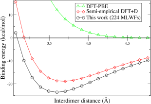
Figure 11: Binding energy curves for H₂Pc dimer in the S configuration (vertically displaced) versus intermolecular distance obtained with the various methods.

In the case of CuPc dimer (vertically displaced S configuration) we again do not use the valence manifold of 390 MLWFs per dimer (195 MLWFs per molecule: 98 spin up and 97 spin down), but instead use a larger manifold of MLWFs. We note that the dimer configuration used here does not correspond to any phases CuPc is observed in experimentally, but was used for illustrative purposes as it is the simplest one. This is a spin-polarized system, so a different set of MLWFs is required for spin up/down electrons, yielding a total of 234 singly occupied MLWFs per molecule (117 for every spin channel). There are 10 $d$-like MLWFs (five for every spin channel) centred on each copper atom, and $s$-like MLWFs on bonds and nitrogens. The MLWFs corresponding to spin up and spin down electrons have essentially the same centres for the same bonds or atoms (Fig. 12).

In such cases, where some Wannier functions centres are very closely centred, it would be incorrect to consider them as separate fragments since this would violate the fundamental assumption of the ALL method, that it is valid for non-overlapping fragments only. This can be understood from the fact that Eq. (13) is strongly non-linear, so adding the contributions of overlapping density fragments does not give the same result as summing the densities beforehand. As a result, Silvestrelli’s method severely overbinds the dimer ($\sim-108$ kcal/mol), demonstrating that the method breaks down for overlapping fragments.

We alleviate this problem by amalgamating all the centres and spreads of the closely placed MLWFs (in this case the $d$-like MLWFs on Cu) into one MLWF with a centre and spread given by the arithmetic mean of the closely placed MLWFs, and occupancies given by the sum of the separate MLWFs. The criterion for amalgamating MLWFs can be automated such that MLWFs less than a particular threshold distance apart are combined. In our case, we used a value of 0.1 Å for this threshold, which had the desired effect of including the $d$-like orbitals on Cu in the amalgamation procedure, while leaving all other MLWFs in the system unaffected.

In Fig. 13 we compare the binding energy curves obtained using DFT+D to our modified method (now including the amalgamation of closely-overlapping MLWFs) using a larger manifold of 468 MLWFs per dimer. This gives much more sensible results, with a binding energy of $-27.22$ kcal/mol and an equilibrium separation of 3.57 Å, in fair agreement with DFT+D, which gives $-22.21$ kcal/mol and 3.63 Å, respectively. These values are in reasonable agreement with those for H₂Pc (as obtained using our method above), and also with those obtained with other methods for other metal phthalocyanines (NiPc and MgPc calculated with the TS-vdW scheme in Ref. Marom et al., 2010 using the PBE funtional).

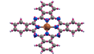
Figure 12: Copper phthalocyanine (CuPc) molecule and its 234 MLWF centres, again including anti-bonding states. Colours as in Fig. 10, with copper shown by the large brown sphere in the centre. There are $s$-symmetry MLWFs on every bond and atom except for copper, $p$-like MLWFs on the carbons and 5 $d$-symmetry MLWFs on the copper atom. Now there are no $p$-like orbitals on any nitrogen atom as for H₂Pc.

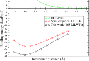
Figure 13: Binding energy curves for the CuPc dimer in the S configuration (vertically displaced) obtained using the various methods.

IV.7 Intermolecular $C_{6}$ coefficients

It is expedient to define effective intermolecular $C_{6}$ coefficients,

$$C_{6{\rm eff}}=\frac{1}{2}\sum_{n,l}C_{6nl},$$ (24)

where only intermolecular terms are summed over, i.e., $n$ and $l$ correspond to MLWFs on different molecules, and the factor of $1/2$ accounts for double-counting. In Table 3, we compare our values to those of the original method of Silvestrelli, benchmark dispersion-corrected MP2 calculations (MP2+$\Delta$vdW) and reference results obtained using the Dipole Oscillator Strength Distribution (DOSD) approach, given in the database of Ref. Tkatchenko et al., 2009.

As previously discussed in Ref. Silvestrelli, 2009a, comparison with reference values is made somewhat difficult by the fact that they are obtained by fitting to experimental data and hence also include higher-order terms ($C_{8}$, $C_{10}$) in an effective manner.

Taking the reference values as a benchmark, it can be seen from Table 3 that, for the systems under consideration, there is no clear or systematic improvement in calculated effective $C_{6}$ coefficients with our modifications to Silvestrelli’s approach as compared to Silvestrelli’s original approach: in the case of ethene the original method compares more favourably, while in the case of the benzene dimers our approach performs much better. In spite of this, however, it is worth noting that our approach (as shown earlier) significantly improves the values obtained for equilibrium separations and binding energies, as compared to CCSD(T), for all systems considered for which we have access to CCSD(T) results.

System	$C_{6}$ ($E_{h}a_{0}^{6}$)
	Silvestrelli	This work	MP2+$\Delta$vdW	pseudo-DOSD
Argon	92.4	92.4	76.1	64.3
Methane	99.1	99.1	119	130
Ethene	275	261	328	300
Benzene S	2727	1288	2364	1723
Benzene PD	2727	1284	2364	1723
Benzene T	2769	1262	2364	1723

Table 3: Effective intermolecular $C_{6}$ coefficients. Dispersion-corrected MP2 (MP2+$\Delta$vdW) and reference values are drawn from Ref. Tkatchenko et al., 2009. For the argon and methane dimers, our approach is identical to the original method of Silvestrelli. The differences between the values reported in the first column (Silvestrelli) and those in Ref. Silvestrelli, 2009a are attributable to the different calculational details such as choice of exchange and correlation functional, simulation cell size and plane-wave energy cutoff.

IV.8 Sensitivity to cutoff radius $r_{c}$

The sensitivity of the binding energy on the cutoff radius $r_{c}$ in Eq. 16 was tested on the S configuration of the benzene dimer with 18 MLWFs per molecule (Fig. 14). Even small changes of 1% in the cutoff radius result in significant changes in the binding energy curves, with the binding energy and equilibrium distance varying by 6-8% and 0.2-0.8% respectively. For larger changes in $r_{c}$, the method breaks down, as the energy changes are unphysically large. Although the cutoff radius is physically justified Andersson, Langreth, and Lundqvist (1996), this strong dependence of the vdW correction on it is a weakness of the method.

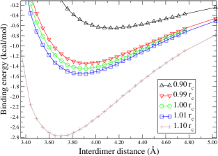
Figure 14: Binding energy curve for the benzene dimer in the S configuration for various values of $r_{c}$ using our modified method with 18 MLWFs per molecule.

IV.9 Approximations to the density

In the original method of Silvestrelli, the KS density is approximated by replacing all real MLWFs with hydrogenic $s$ wavefunctions $w_{n}^{H}({\bf r})$ given by Eq. (15); for the purpose of calulating the $C_{6}$ coefficients, the electronic charge density of the system is, therefore, effectively approximated as

$$\rho_{\rm s}({\bf r})=\sum_{n=1}^{N_{\rm occ}}|w_{n}^{H}({\bf r})|^{2}.$$ (25)

In the modified method presented here, in which the MLWFs are constructed using a manifold of the KS states beyond just the occupied orbitals, there are two levels of approximation to the charge density. First, the off-diagonal component $\rho_{OD}({\bf r})$ is neglected from Eq. (10) and, second, the “hydrogenic” approximation of the original approach is applied, whereby the disentangled Wannier functions, $w_{n}^{\rm dis}({\bf r})$, are replaced by hydrogenic orbitals, $w_{n}^{H}({\bf r})$, of the same center and spread. In our method, therefore, the density is approximated as

$$\rho_{\rm dis}({\bf r})=\sum_{n=1}^{N}f^{w}_{nn}|w_{n}^{H}({\bf r})|^{2},$$ (26)

where $N$ is now the of total number of fragments, after the splitting of $p$-like orbitals or amalgamation of co-centric MLWFs has been performed. We consider each of these approximations in turn for a typical system, the benzene molecule.

The XCrySDenKokalj (2003) package was used to generate the isosurface plots referred to in this Section.

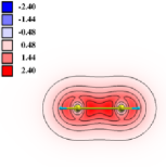
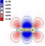
Figure 15: Density profile on a plane parallel to a C-C bond ($xz$-plane) in a benzene molecule. Left: the original Kohn-Sham density $\rho({\bf r})$ from the plane-wave DFT calculation. Right: The off-diagonal component $\rho_{OD}({\bf r})$ of the density (see Eq. (10)) when a disentangled manifold is used to construct $N_{\textrm{dis}}=18$ MLWFs. Note the much-reduced scale compared to that of the total density. The units are Å^-3.

In Fig. 15 we show density isosurface plots for the KS density $\rho({\bf r})$ (left) and the off-diagonal density $\rho_{\rm OD}({\bf r})$ (right), which emphasises that the latter is uniformly small in magnitude, comprising only a small fraction of the total density ($\sim 5-7\%$), as a result of the exponential localisation of the MLWFs.

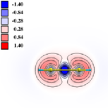
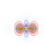
Figure 16: Density difference isosurface plots showing the difference $\rho({\bf r})-\rho_{\rm s}({\bf r})$ between the KS density and the approximate “hydrogenic” density of the original Silvestrelli approach (Eq. (25)). Left: cross-section through a “single” bond. Right: cross-section through a “double” bond.

In Fig. 16 we show the difference between the KS density $\rho({\bf r})$ and the “hydrogenic” approximation $\rho_{\rm s}({\bf r})$ of the original Silvestrelli method (Eq. (25)) for two of the C-C bonds in benzene: on the left a “single” bond; on the right a “double” bond. These two bonds only differ because of the symmetry-breaking inherent in the MLWF construction when just the valence states are used. We see that the density associated with the $\pi$-bond is not well represented in either case.

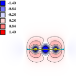
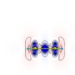
Figure 17: Density difference isosurface plots, on the same plane as in Fig. 15, showing the difference $\rho({\bf r})-\rho_{\rm dis}({\bf r})$ between the KS density and the “hydrogenic” density of our method when a disentangled set of MLWFs is used (Eq. (26)). Left: without splitting of $p$-like states; right: with splitting of $p$-like states into two $s$-like states. The mean difference with the KS density compared to the original Silvestrelli’s method is reduced overall for both cases, but even more in the case of $p$-splitting.

Finally, in Fig. 17, we show the difference between the KS density $\rho({\bf r})$ and that of our modified method $\rho_{\rm dis}({\bf r})$ (Eq. (26)) with 18 MLWFs obtained by disentanglement from a larger manifold. The left-hand plot is without splitting the $p$-like states, and the right-hand plot is with (as described in Sec. III).

We see that while this introduces small regions where the density differs significantly (right at the MLWF centers), everywhere else it is overall an improvement, producing a better representation of the density compared to the original Silvestrelli’s method, especially in the case of $p$-splitting.

In summary, discarding the off-diagonal component of the density (in the case of disentangled MLWFs) is a relatively minor approximation, and has a considerably smaller effect than approximating the density in various ways using hydrogenic orbitals, the latter being inherent to both our approach and the original approach of Silvestrelli. The maximum difference between the KS density $\rho({\bf r})$ and the density in our method is reduced by $\sim 23\%$ and the minimum difference by $\sim 5\%$, compared to the difference between the KS density and the density in Silvestrelli’s method.

IV.10 Sensitivity to energy window $E_{{\rm win}}$

To use our modifications to Silvestrelli’s method, the disentanglement procedure has to be used in the construction of Wannier functions, as outlined in the Methods section. Because including ever more high-energy plane-wave states inevitably allows extra variational freedom in the construction of the MLWFs, we find that the precise values of the MLWF spreads are sensitive to the outer energy window used for the disentanglement. Specifically as $E_{{\rm win}}$ is increased, the MLWFs become more localised (their spreads decrease). As a result, the vdW energy is also affected by the choice of $E_{{\rm win}}$.

In this work we have chosen throughout to estimate an appropriate energy window using

$$E_{{\rm win}}=\epsilon_{{\rm LUMO}}+\alpha(\epsilon_{{\rm HOMO}}-\epsilon_{0})$$ (27)

where $\alpha$ is a factor used to scale the valence energy bandwidth. This is motivated by the idea that to enable us to restore the symmetry, we need to include the antibonding counterparts to the valence states, without including too large a number of irrelevant higher-lying unbound states. Eq. (27) is an attempt to estimate the range of energies spanned by these antibonding states. In Fig. 18 we show the dependence of the vdW binding energy curves for the benzene dimer in the S configuration on $\alpha$. While there is considerable variation for too-small $\alpha$, we find that for values beyond 0.4, the curves vary only a rather small amount with $\alpha$; As long as a value of $\alpha$ around this value is chosen, it should yield reasonable results, suggesting the extra degree of empiricism introduced by this procedure is relatively limited in scale. The value of $\alpha$ was set to 0.4 in all the other calculations in this work.

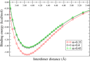
Figure 18: Binding energy curve for the benzene dimer in the S configuration for various values of $\alpha$ using our modified method with 18 MLWFs per molecule.

V Conclusion

We conclude that Silvestrelli’s method is computationally efficient and very easy to implement for small systems where initial guesses for the Wannier centres can be specified. However, there is a very strong dependence of the calculated vdW energy on the position and spread of the Wannier centres, and these are not always as unique as one might hope. Symmetry-breaking, often induced by considering only the valence manifold in the construction of the MLWFs, may introduce arbitary dependence on initial guesses in a way that significantly affect the vdW energy. We have shown that arbitrarily-broken symmetries may often be restored by increasing the number of Wannier functions used and generating them with a suitably-chosen range of the conduction states as well as the valence states. This necessitates the inclusion of occupancies in the formalism. We note that in cases where no symmetries are restored when we use more MLWFs, as in the example of ethene, it is the better localisation of the MLWFs that may be responsible for improved vdW energies, since the method is based on pairwise summation of well-separated fragments.

Particularly, in cases with a larger number of Wannier functions, we have shown that the approximation implicit in replacing the true Wannier functions with hydrogenic $s$-orbitals may not always yield an accurate representation of the electronic density, and have shown how in cases where there is $p$-like symmetry, it is better to substitute the $p$-symmetry functions with two $s$-like functions. By considering the problems associated with applying these adapted methods to larger systems such as H₂Pc and CuPc, we have demonstrated that the approach is not necessarily a good candidate for studying larger systems, where specifying initial guesses for a large number of non-trivial MLWFs may be difficult; chemical insight for the form of these higher-lying states has to be employed, but becomes more difficult for even larger systems. In the case of copper phthalocyanine, we showed that MLWFs that are centred effectively at the same point (such as the five $d$-like MLWFs on each Cu atom) cannot be treated as separate fragments of density; they should instead be amalgamated into one fragment of density of an averaged centre and spread and summed occupancies. The reason for this is that the method is valid only in the limit of well-separated fragments. Finally, we have demonstrated that there is also a strong dependence of the vdW energy on the cutoff radius used in the integral of Eq. (16), and although the value used is justified on physical grounds, it nevertheless represents something of an adjustable parameter with considerable influence on the results obtained. Overall, we conclude that while Silvestrelli’s method suffers from several drawbacks, it can be made rather accurate once modifications are applied to it (albeit with the introduction of further empirical character); these improvements, and Silvestrelli’s method in general, however, may be less suitable for more structurally complex, large-scale systems, for which alternative methods that are more fully ab initio may be desirable.