An elementary formula for computing shape derivatives of EFIE system matrix

Abstract

We derive analytical shape derivative formulas of the system matrix representing electric field integral equation discretized with Raviart-Thomas basis functions. The arising integrals are easy to compute with similar methods as the entries of the original system matrix. The results are compared to derivatives computed with automatic differentiation technique and finite differences, and are found to be in excellent agreement.

1 Introduction

The adjoint variable methods based on shape gradients have recently gained significant attention in the shape optimization of microwave devices [9, 15]. The main reason for such an interest is that the adjoint variable approach eases significantly the computational burden of the optimization process: computing the gradient of the objective requires only one solve of the governing state equations, and in addition, at most one solve of the adjoint problem.

The adjoint variable methods rely on the availability of the derivatives of the system matrix with respect to the control parameters. Traditionally these derivatives have been computed with finite difference (FD) formulas. The main drawback of this approach is that the accuracy greatly depends on the step length parameter, which has to be carefully chosen in order to find a suitable balance between round off and truncation errors.

Use of the automatic differentiation (AD) was proposed in [15] to compute the derivatives of the system matrix arising from a method of moments discretization of the electric field integral equation (EFIE). The method was applied to antenna shape optimization problems in [15, 16]. AD computes the exact derivatives of the computer code, but there are some complications involved.

AD can be implemented either as a source transformation tool, or using operator overloading. Source transformation tools are complicated to implement, and existing tools are available only for some programming languages. While using these tools, one may be forced to restructure the code, and avoid such features of the programming language that are not supported. Tools based on the operator overloading are more simple to implement, but not all programming languages support operator overloading. Moreover, there is some execution overhead related to this approach. In both cases, AD has to be applied also to all subroutines that are called from the code, which may present difficulties if one wishes to use any external libraries.

The electric field integral equation is a widely used method to compute scattering of time harmonic electromagnetic field from perfectly electrically conducting (PEC) bodies and surfaces [10, 3, 8]. In this paper we derive simple analytical formulas for calculating the system matrix derivatives of the discretized EFIE system. The arising integrals are such that they are easy to compute using methods similar to those used to calculate the elements of the original system matrix. The results are compared against derivatives calculated using automatic differentiation and difference formulas.

We employ the lowest order Raviart-Thomas (RT) basis functions [13] in the discretization. They are almost identical to the Rao-Wilton-Glisson (RWG) basis functions [12], which are the usual choice to discretize the EFIE, except that usually the RWG functions are scaled with the length of the edge which they are related to.

The shape derivatives of the electromagnetic field solution together with the far field pattern has been characterized and analyzed in [4, 5, 11]. Contrary to these works, we consider differentiation of the discretized system, and utilize the adjoint variable method.

2 Preliminaries

Let $S$ be a surface with or without boundary in $\mathbb{R}^{3}$ and $\mathcal{T}$ its triangulation. It can be a boundary of a some sufficiently regular open domain in $\mathbb{R}^{3}$, in which case it models the scattering object. If it is not a boundary of any set, but it otherwise exhibits sufficient regularity, it acts as a model for a thin perfectly conducting screen.

In what follows, $\mathrm{RT}(\mathcal{T})$ denotes the space spanned by the lowest order Raviart-Thomas (RT) basis functions on $\mathcal{T}$, $\nabla_{s}\cdot$ denotes the surface divergence, and $\nabla_{s}$ denotes the surface gradient.

In the EFIE the unknown function to be solved is, roughly speaking, the equivalent surface current $\mathbf{J}=\hat{\mathbf{n}}\times\mathbf{H}$, where $\hat{\mathbf{n}}$ is the surface unit normal and $\mathbf{H}$ is the total magnetic field. The source term in the equation is the incident electric field denoted by $\mathbf{E}_{p}$.

The current $\mathbf{J}$ satisfies the Rumsey reaction principle [8, 2, 1, 14]:

Find $\mathbf{J}\in H^{-1/2}_{\times}(\nabla_{s}\cdot;S)$ s.t.

$$\frac{i}{\omega\epsilon}\int_{S}\nabla_{s}\cdot\mathbf{u}(x) \int_{S}g_{k}(x-y)\nabla_{s}\cdot\mathbf{J}(y)dydx-i\omega\mu\int_{S}\mathbf{u}(x)\cdot\int_{S}g_{k}(x-y)\mathbf{J}(y)dydx$$

$$=\int_{S}\mathbf{u}(x)\cdot\mathbf{E}_{p}(x)dx\quad\forall\mathbf{u}\in H^{-1/2}_{\times}(\nabla_{s}\cdot;S).$$ (1)

Here $g_{k}$ is the fundamental solution of the Helmholtz equation:

$$g_{k}(x)=\frac{e^{ik|x|}}{4\pi|x|},$$ (2)

and $\nabla_{s}\cdot$ is the surface divergence. We denote the Euclidean norm of $x\in\mathbb{R}^{3}$ by $|x|$.

For detailed treatment of the space $H^{-1/2}_{\times}(\nabla_{s}\cdot;S)$ and the above equation we refer to [2]. We note that the integrals in (1) should be interpreted as a certain duality pairing, but at the discrete level they are proper integrals.

After discretizing the equation (1) we arrive to the following finite dimensional variational problem:

Find $\mathbf{J}_{h}\in\mathrm{RT}$ such that

$$a(\mathbf{v},\mathbf{J}_{h})=\int_{S}\mathbf{v}(x)\cdot\mathbf{E}_{p}(x)dx,\quad\forall\mathbf{v}\in\mathrm{RT}(\mathcal{T}),$$ (3)

where the bilinear form $a$ is given by

$$a(\mathbf{v},\mathbf{u})= \frac{i}{\omega\epsilon}\int_{S}\nabla_{s}\cdot\mathbf{v}(x)\int_{S}g_{k}(x-y)\nabla_{s}\cdot\mathbf{u}(y)dydx-$$

$$i\omega\mu\int_{S}\mathbf{v}(x)\cdot\int_{S}g_{k}(x-y)\mathbf{u}(y)dydx.$$ (4)

We denote the corresponding linear system of equations of (3) by

$$\boldsymbol{\mathrm{A}}\boldsymbol{\mathrm{x}}=\boldsymbol{\mathrm{b}}.$$ (5)

Let $T_{p},T_{q}\in\mathcal{T}$, $\mathbf{u},\mathbf{v}\in\mathrm{RT}(\mathcal{T})$, and $\mathrm{supp}\,\mathbf{u}$ and $\mathrm{supp}\,\mathbf{v}$ intersect $T_{p}$ and $T_{q}$, resp. In order to compute the entries of $\boldsymbol{\mathrm{A}}$ one needs to compute integrals of type

$$I_{1}(\mathbf{u},\mathbf{v};{T_{p}},{T_{q}}) =\int_{T_{q}}\mathbf{v}(x)\cdot\int_{T_{p}}g_{k}(x-y)\mathbf{u}(y)dydx,$$ (6)

$$I_{2}(\mathbf{u},\mathbf{v};{T_{p}},{T_{q}}) =\int_{T_{q}}\nabla_{s}\cdot\mathbf{v}(x)\int_{T_{p}}g_{k}(x-y)\nabla_{s}\cdot\mathbf{u}(y)dydx.$$ (7)

We denote the usual interpolating nodal piecewise first order polynomials on $S$ associated with $\mathcal{T}$ by $(\lambda_{m})_{m=1}^{N}$, where $N$ is the number of vertices in $\mathcal{T}$.

2.1 Adjoint variable methods for the EFIE system

Let $\boldsymbol{\alpha}$ be the vector of design variables, and $\mathcal{J}(\boldsymbol{\alpha},\boldsymbol{\mathrm{x}}(\boldsymbol{\alpha}))$ be a real valued objective function. In general, real valued functions are not differentiable with respect to complex arguments in the conventional complex analytic sense. Therefore we differentiate $\mathcal{J}$ separately with respect to the real and imaginary parts of the variables $\boldsymbol{\mathrm{x}}$:

$$\frac{\rm d\mathcal{J}}{\rm d\alpha_{k}}=\frac{\partial\mathcal{J}}{\partial\alpha_{k}}+\frac{\partial\mathcal{J}}{\partial\Re\boldsymbol{\mathrm{x}}}\frac{\partial\Re\boldsymbol{\mathrm{x}}}{\partial\alpha_{k}}+\frac{\partial\mathcal{J}}{\partial\Im\boldsymbol{\mathrm{x}}}\frac{\partial\Im\boldsymbol{\mathrm{x}}}{\partial\alpha_{k}}.$$ (8)

Here $\partial\mathcal{J}/\partial\alpha_{k}$ reflects the explicit dependence of $\mathcal{J}$ on the design.

The convention $\nabla_{\boldsymbol{\mathrm{x}}}\mathcal{J}:=\nabla_{\Re\boldsymbol{\mathrm{x}}}\mathcal{J}+i\nabla_{\Im\boldsymbol{\mathrm{x}}}\mathcal{J}$ will be used to simplify notation. It can be easily checked that equation (8) can now be written as

$$\frac{\rm d\mathcal{J}}{\rm d\alpha_{k}}=\frac{\partial\mathcal{J}}{\partial\alpha_{k}}+\Re\left[(\nabla_{\boldsymbol{\mathrm{x}}}\mathcal{J})^{H}\frac{\partial\boldsymbol{\mathrm{x}}}{\partial\alpha_{k}}\right].$$ (9)

By differentiating the state relation $\boldsymbol{\mathrm{A}}\boldsymbol{\mathrm{x}}=\boldsymbol{\mathrm{b}}$, we obtain

$$\boldsymbol{\mathrm{A}}\frac{\partial\boldsymbol{\mathrm{x}}}{\partial\alpha_{k}}=-\frac{\partial\boldsymbol{\mathrm{A}}}{\partial\alpha_{k}}\boldsymbol{\mathrm{x}}+\frac{\partial\boldsymbol{\mathrm{b}}}{\partial\alpha_{k}}.$$ (10)

In the so called direct differentiation approach, the derivatives $\partial\boldsymbol{\mathrm{x}}/\partial\alpha_{k}$ are solved from (10), and (9) is used to compute the gradient of the objective function. However, the right hand side of (10) is different for each design variable, which makes this approach rather inefficient.

By introducing the adjoint problem

$$A^{H}\gamma=\nabla_{\boldsymbol{\mathrm{x}}}\mathcal{J},$$ (11)

and using (10), equation (9) can be written as

$$\frac{\partial\mathcal{J}}{\partial\alpha_{k}} =\frac{\partial\mathcal{J}}{\partial\alpha_{k}}+\Re\left[(\nabla_{\boldsymbol{\mathrm{x}}}\mathcal{J})^{H}\boldsymbol{\mathrm{A}}^{-1}\left(\frac{\partial\boldsymbol{\mathrm{b}}}{\partial\alpha_{k}}-\frac{\partial\boldsymbol{\mathrm{A}}}{\partial\alpha_{k}}\boldsymbol{\mathrm{x}}\right)\right]$$ (12)

$$=\frac{\partial\mathcal{J}}{\partial\alpha_{k}}+\Re\left[(\gamma^{H}\left(\frac{\partial\boldsymbol{\mathrm{b}}}{\partial\alpha_{k}}-\frac{\partial\boldsymbol{\mathrm{A}}}{\partial\alpha_{k}}\boldsymbol{\mathrm{x}}\right)\right].$$ (13)

In the adjoint variable method, equation (11) is solved for $\gamma$, and equation (13) is used to compute the gradient of the objective. Notice that the adjoint problem (11) does not depend on the design, and therefore $\gamma$ is the same for all design variables. In case of some particular objective functions (see e.g. [9]), the adjoint vector $\gamma$ can be immediately obtained from the solution vector $\boldsymbol{\mathrm{x}}$, and one does not have to solve the adjoint problem at all.

In any case, the derivatives of the right hand side and the system matrix with respect to the design variables are required. This paper presents analytical formulas, which can be used to compute them efficiently in the case where $\boldsymbol{\mathrm{A}}$ is a system matrix arising from the EFIE formulation (3).

3 The derivative formulas

We define the shape deforming mapping with the aid of the global nodal shape functions $\lambda_{m}$ as follows.

Let $\boldsymbol{\tau}\in\mathbb{R}^{3}$ be a vector and $0\leq s<1$. We define the deformation mapping $F_{s}^{m}$ associated with node $m$ by

$$F_{s}^{m}(x)=x+s\boldsymbol{\tau}\lambda_{m}(x).$$ (14)

Note that the domain of $F_{s}^{m}$ is the whole of $S$. We shall drop the superscript $m$ from $F_{s}^{m}$ whenever it does not cause confusion.

Let $K$ be a triangle in $\mathbb{R}^{2}$ and $F$ a diffeomorphism from $K$ to its image. We define the Piola transform $\mathop{\mathcal{P}_{F}}$ associated with $F$ by

$$\mathop{\mathcal{P}_{F}}\mathbf{u}=\frac{1}{\det F^{\prime}}F^{\prime}\mathbf{u}\circ F^{-1},$$ (15)

which maps smooth sections of the tangent bundle of $K$ to those of $F(K)$. Here the Jacobian of $F$ by is denoted by $F^{\prime}$. We note that the divergence of the Piola transformed function $\mathbf{u}$ is given by

$$\nabla_{s}\cdot\mathop{\mathcal{P}_{F}}\mathbf{u}=\frac{1}{\det F^{\prime}}(\nabla_{s}\cdot\mathbf{u})\circ F^{-1}.$$ (16)

This simplifies the calculations greatly, as we shall see.

The Raviart-Thomas basis functions can be defined using the Piola transform and reference element as follows. Let $\widehat{K}$ be the standard 2-simplex

$$\{(x,y)\in\mathbb{R}^{2}:\,0<x,\,0<y,\,\mathrm{and}\,0<x+y<1\}$$

and define functions $\widehat{\mathbf{u}}_{i}$ on $\widehat{K}$ by

$$\begin{cases}\widehat{\mathbf{u}}_{1}(x,y)=[x,\,1-y]^{T},&\\ \widehat{\mathbf{u}}_{2}(x,y)=[x,\,y]^{T}&\mathrm{and}\\ \widehat{\mathbf{u}}_{3}(x,y)=[1-x,\,y]^{T}.\end{cases}$$ (17)

Now the restriction of an arbitrary $\mathbf{u}\in\mathrm{RT}(\mathcal{T})$ to the triangle $K$ is a Piola transform of some $\widehat{\mathbf{u}}_{i}$ ie.

$$\mathbf{u}=\mathop{\mathcal{P}_{F_{K}}}\widehat{\mathbf{u}}_{i}$$

for some $i\in\{1,2,3\}$, where $F_{K}$ is the affine mapping which maps $\widehat{K}$ to $K$. We note that the the determinant of $F_{K}^{\prime}$ is given by $\det F_{K}^{\prime}=\pm 2|K|$, where $|K|$ is the area of $K$ and the sign is determined by its orientation.

The main objects of interest in this work are the derivatives

$$\frac{\partial}{\partial s}I_{m}(\mathop{\mathcal{P}_{F_{S}}}\mathbf{u},\mathop{\mathcal{P}_{F_{s}}}\mathbf{v};F_{s}({T_{p}}),F_{s}({T_{q}}))\big{|}_{s=0},\quad m=1,2.$$ (18)

To start with, we note that

$$I_{1} (\mathop{\mathcal{P}_{F_{s}}}\mathbf{u},\mathop{\mathcal{P}_{F_{s}}}\mathbf{v};F_{s}({T_{p}}),F_{s}({T_{q}}))=$$

$$\int_{F_{s}({T_{q}})}\int_{F_{s}({T_{p}})}\frac{F_{s}^{\prime}(x)\mathbf{v}\circ F_{s}^{-1}(x)}{\det F_{s}^{\prime}(x)}\cdot\frac{F_{s}^{\prime}(y)\mathbf{u}\circ F_{s}^{-1}(y)}{\det F_{s}^{\prime}(y)}g_{k}(x-y)dydx=$$

$$\int_{T_{q}}\int_{T_{p}}F_{s}^{\prime}(x)\mathbf{v}(x)\cdot F_{s}^{\prime}(y)\mathbf{u}(y)g_{k}(F_{s}(x)-F_{s}(y))dydx.$$ (19)

and

$$I_{2} (\mathop{\mathcal{P}_{F_{s}}}\mathbf{u},\mathop{\mathcal{P}_{F_{s}}}\mathbf{v};F_{s}({T_{p}}),F_{s}({T_{q}}))=$$

$$\int_{F_{s}({T_{q}})}\int_{F_{s}({T_{p}})}\frac{(\nabla_{s}\cdot\mathbf{v})\circ F_{s}^{-1}(x)}{\det F_{s}^{\prime}(x)}\cdot\frac{(\nabla_{s}\cdot\mathbf{u})\circ F_{s}^{-1}(y)}{\det F_{s}^{\prime}(y)}g_{k}(x-y)dydx=$$

$$\int_{T_{q}}\int_{T_{p}}\nabla_{s}\cdot\mathbf{v}(x)\cdot\nabla_{s}\cdot\mathbf{u}(y)g_{k}(F_{s}(x)-F_{s}(y))dydx.$$ (20)

For conciseness, we denote $I_{m}^{s}=I_{m}(\mathop{\mathcal{P}_{F_{s}}}\mathbf{u},\mathop{\mathcal{P}_{F_{s}}}\mathbf{v};F_{s}({T_{p}}),F_{s}({T_{q}}))$.

Looking at (19) and (20) we find that we only need to compute derivatives of $g_{k}$ and $F^{\prime}_{s}$ wrt. $s$.

Lemma 1.

Let $F_{s}^{m}$ be given by Eq. (14). It holds that

$$\frac{\partial}{\partial s}|F_{s}^{m}(x)-F_{s}^{m}(y)|\big{|}_{s=0}=\frac{(x-y)\cdot\boldsymbol{\tau}(\lambda_{m}(x)-\lambda_{m}(y))}{|x-y|}$$ (21)

and

$$\frac{\partial}{\partial s}F_{s}^{\prime}(x)^{T}F_{s}^{\prime}(y)\big{|}_{s=0}=(\boldsymbol{\tau}\nabla_{s}\lambda_{m}(x))^{T}+\boldsymbol{\tau}\nabla_{s}\lambda_{m}(y).$$ (22)

Proof.

Just by calculating

$$|F_{s}^{m}(x)-F_{s}^{m}(y)|^{2} =|x-y+s\boldsymbol{\tau}\left(\lambda_{m}(x)-\lambda_{m}(y)\right)|^{2}$$

$$=\,A+2s(x-y)\cdot\boldsymbol{\tau}(\lambda_{m}(x)-\lambda_{m}(y))+Bs^{2},$$

where $A$ and $B$ are constants wrt. $s$. By using chain rule, the first assertion follows.

For the second formula, we note that

$$F_{s}^{\prime}(x)=I+s\boldsymbol{\tau}\nabla_{s}\lambda_{m}(x)$$ (23)

and the assertion is obvious. ∎

Using the above results we have the shape derivative of the kernel $g_{k}$ as

$$\frac{\partial}{\partial s}g_{k}(F_{s}(x)-F_{s}(y))\big{|}_{s=0}=g_{k}(x-y)\left(ik-\frac{1}{|x-y|}\right)\frac{(x-y)\cdot\boldsymbol{\tau}(\lambda_{m}(x)-\lambda_{m}(y))}{|x-y|}.$$ (24)

Furthermore, this can be simplified to

$$\frac{\partial}{\partial s}g_{k}(F_{s}(x)-F_{s}(y))\big{|}_{s=0}=\boldsymbol{\tau}\cdot(\nabla g_{k})(x-y)(\lambda_{m}(x)-\lambda_{m}(y)).$$

Thus, we immediately get the formula

$$\boxed{\frac{\partial}{\partial s}I_{2}^{s}=\int_{T_{q}}\int_{T_{p}}\nabla_{s}\cdot\mathbf{v}(x)\nabla_{s}\cdot\mathbf{u}(y)\boldsymbol{\tau}\cdot(\nabla g_{k})(x-y)\left(\lambda_{m}(x)-\lambda_{m}(y)\right)dydx.}$$ (25)

The derivative $\frac{\partial}{\partial s}I_{1}^{s}$ is only slightly more complicated; it is obtained by an application of the Leibniz’s rule:

$$\frac{\partial}{\partial s}I_{1}^{s} =\int_{T_{q}}\int_{T_{p}}\left(\frac{\partial}{\partial s}\mathbf{v}(x)\cdot F_{s}^{\prime}(x)^{T}F_{S}^{\prime}(y)\mathbf{u}(y)\right)g_{k}(x-y)+$$

$$\hskip 28.45274pt\mathbf{v}(x)\cdot\mathbf{u}(y)\frac{\partial}{\partial s}g_{k}(F_{s}(x)-F_{s}(y))dydx.$$ (26)

Thus we obtain

$$\frac{\partial}{\partial s}I_{1}^{s} =\int_{T_{q}}\int_{T_{p}}\mathbf{v}(x)\cdot\left((\boldsymbol{\tau}\nabla_{s}\lambda_{m}(x))^{T}+\boldsymbol{\tau}\nabla_{s}\lambda_{m}(y)\right)\cdot\mathbf{u}(y)g_{k}(x-y)+$$

$$\hskip 28.45274pt\mathbf{v}(x)\cdot\mathbf{u}(y)\boldsymbol{\tau}\cdot(\nabla g_{k})(x-y)\left(\lambda_{m}(x)-\lambda_{m}(y)\right)dydx.$$ (27)

4 Numerical verifications

We compare the results given by the formulas (27) and (25) to the values of derivative computed with difference formulas and automatic differentiation applied to numerical code which computes $I_{m}^{s}$ at $s=0$.

To start with, we note that the integrals (27) and (25) are singular when the closures of $T_{p}$ and $T_{q}$ intersect. Thus we manipulate the expressions in such a way that we can directly apply singularity subtraction methods to compute them.

The singularity subtraction method is designed to calculate singular integrals of the form

$$\int v(x)\int K(x-y)u(y)dydx,$$ (28)

where $K$ is singular at $0$. The idea is to express $K$ as a sum of singular $K_{s}$ and a function $K_{b}$ bounded at $0$, in such a way that $\int K_{s}(x-y)v(x)dx$ can be evaluated analytically, and $\int K_{b}(x-y)v(x)dx$ integrates easily with numerical quadratures. In this paper, we use the same quadrature to integrate $K=K_{s}+K_{b}$ wrt. $y$ and the inner integral with kernel $K_{b}$ wrt. $x$. Note that $\int K_{b}(x-y)v(x)dx$ is integrated analytically.

Looking at equations (25) and (27) we observe that we only need to compute integrals of type

$$\begin{cases}\displaystyle\int\nabla_{s}\cdot\mathbf{v}(x)\int\boldsymbol{\tau}\cdot\nabla_{x}g_{k}(x-y)\left(\lambda_{m}(x)-\lambda_{m}(y)\right)\nabla_{s}\cdot\mathbf{u}(y)dydx&\\ \displaystyle\int\mathbf{v}(x)\cdot\int\boldsymbol{\tau}\cdot\nabla_{x}g_{k}(x-y)\left(\lambda_{m}(x)-\lambda_{m}(y)\right)\mathbf{u}(y)dydx&\\ \displaystyle\int\int\mathbf{v}(x)\cdot T(x,y)\mathbf{u}(y)g_{k}(x-y)dydx\end{cases}$$ (29)

Here $T(x,y)=(\boldsymbol{\tau}\nabla_{s}\lambda_{m}(x))^{T}+\boldsymbol{\tau}\nabla_{s}\lambda_{m}(y)$. Looking at these, we find that they can be calculated using singularity subtraction techniques discussed e.g. in [7].

In the following we shall compare numerical values of

$$\frac{\partial}{\partial s}I_{m}^{s}\big{|}_{s=0},\quad m=1,2$$ (30)

calculated with automatic differentiation applied to the singularity subtraction technique, analytical formulas introduced here, and forward difference formula. We inspect these values with four different triangle configurations that occur in computations: the triangles $T_{p}$ and $T_{q}$ do not touch, they share a vertex, they share an edge, and the triangles are equal. These four cases are presented in Figure 1.

The automatic differentiation algorithm generates code which computes the derivatives of (30). The non-differentiated code calculates the system matrix contributions of two triangles with singularity subtraction technique by removing the two most singular terms from the kernel of the EFIE integral. To get directly comparable results, we also subtract two terms when computing the derivatives using analytical formulas. For details and an example where the AD technique is employed in EFIE calculations we refer to [15].

We compute the derivatives of the local system matrix contributions

$$a_{pq}^{s}(\mathbf{u},\mathbf{v})= \frac{i}{\omega\varepsilon}I_{2}(\mathop{\mathcal{P}_{F_{s}}}\mathbf{u},\mathop{\mathcal{P}_{F_{s}}}\mathbf{v};F_{s}(T_{p}),F_{s}(T_{q}))-$$

$$i\omega\mu I_{1}(\mathop{\mathcal{P}_{F_{s}}}\mathbf{u},\mathop{\mathcal{P}_{F_{s}}}\mathbf{v};F_{s}(T_{p}),F_{s}(T_{q})),$$ (31)

where $\mathbf{u}$ and $\mathbf{v}$ vary over three local $\mathrm{RT}$ basis functions on $T_{p}$ and $T_{q}$ respectively, and investigate the effect of changing the number of integration points $n$. The quadrature rules were adapted from [6].

In Tables 5–5 we inspect the sum

$$\Im\sum_{\mathbf{u},\mathbf{v}}\frac{\partial}{\partial s}a_{pq}^{s}(\mathbf{u},\mathbf{v}),$$ (32)

computed with the AD method, analytical formulas and the FD method given by

$$f^{\prime}(s)\approx(f(s+h)-f(s))/h.$$ (33)

The step length parameter was chosen to be $h=10^{-8}$. The reason for presenting only the imaginary part is that it is the most involved integral to compute.

In Tables 5–5 we have the difference in the Frobenius norm of the $3\times 3$ matrices $\frac{\partial}{\partial s}a_{pq}^{s}$ relative to the values computed using the present methods.

We see that the proposed analytical formulas and the automatic differentiation approach produce same results up to numerical precision. Relative difference of the derivatives obtained with the FD method is of the order $10^{-7}$. This is expected, since the forward finite difference formula has a truncation error of the order $\mathcal{O}(h)$.

5 Concluding remarks

We have derived compact analytical formulas to calculate the shape derivatives of the EFIE system matrix arising from RT discretization. The derivatives are easy to implement, since the emerging integrals can be calculated using similar algorithms as the original EFIE system matrix. In this case we used singularity subtraction technique, but the use of the singularity cancellation methods [17] could be possible as well.

We have shown that the shape derivatives are the same, up to numerical precision, as the ones computed using automatic differentiation (AD), if one uses the same techniques to evaluate the arising integrals. On the other hand, AD is known to produce the exact derivatives of the given computer realization. Such derivatives are perfectly consistent with the objective function values, which is very convenient from the optimization perspective. The accuracy of the derivatives is naturally dictated by the utilized numerical methods, and depends heavily for example on the number of points used for the numerical integration.

The analytical formulas offer several benefits over the automatic differentiation approach. Existing AD tools are available only for some programming languages, and while using these tools, one may be forced to restructure the code and avoid some features of the programming language. Moreover, AD has to be applied also to all subroutines that are called from the code, which may present difficulties if one wishes to use any external libraries. Finally, implementing the analytical formula is likely to lead to better computational performance, as one avoids execution overhead related to some AD techniques, and the programmer is free to optimize the code.

The FD derivatives are approximate by nature, and their accuracy greatly depends on the step length parameter. From the numerical results we can conclude that the derivatives computed with the proposed formulas are in agreement with the finite difference derivatives. Use of the analytical formulas is therefore preferred, because the need to choose a step length parameter is avoided.

By having an analytical formula at hand, one is free to use any suitable method for its numerical evaluation. Thus it is easy to make a trade-off between accuracy and computational efficiency. Moreover, the analytical formulas provide a basis for understanding the behaviour of the derivatives.

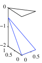
(a) near

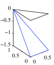
(b) point

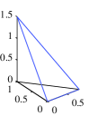
(c) edge

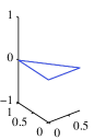
(d) same

Figure 1: Three different configurations of triangles $T_{p}$ and $T_{q}$ triangles. The triangle $T_{q}$ remains still in each of the cases.

Table 1: The imaginary part of $I(\mathbf{u},\mathbf{v})$ defined by the equation (32)

$n$	Analytical	AD	FD
6	2.98169473e+01	2.98169473e+01	2.98169583e+01
16	2.98097099e+01	2.98097099e+01	2.98097110e+01
61	2.98096873e+01	2.98096873e+01	2.98096885e+01
85	2.98096873e+01	2.98096873e+01	2.98096876e+01

(a) near

[point] $n$ Analytical AD FD 6 -6.13463371e+00 -6.13463371e+00 -6.13463194e+00 16 -6.11420678e+00 -6.11420678e+00 -6.11420794e+00 61 -6.11421020e+00 -6.11421020e+00 -6.11421161e+00 85 -6.11416794e+00 -6.11416794e+00 -6.11417224e+00 [edge] $n$ Analytical AD FD 6 -7.84966165e+01 -7.84966165e+01 -7.84966142e+01 16 -7.67762767e+01 -7.67762767e+01 -7.67762887e+01 61 -7.68970360e+01 -7.68970360e+01 -7.68970451e+01 85 -7.68875833e+01 -7.68875833e+01 -7.68875768e+01   [same] $n$ Analytical AD FD 6 -5.98000685e+01 -5.98000685e+01 -5.98000312e+01 16 -5.86918000e+01 -5.86918000e+01 -5.86917977e+01 61 -5.87792043e+01 -5.87792043e+01 -5.87792522e+01 85 -5.87738744e+01 -5.87738744e+01 -5.87738958e+01

Table 2: Relative difference to analytical derivative

(a) near

[point] $n$ AD FD 6 1.07e-15 1.30e-07 16 7.25e-16 9.42e-08 61 2.05e-15 4.73e-08 85 1.24e-15 1.57e-07 [edge] $n$ AD FD 6 5.53e-16 3.51e-08 16 3.21e-15 1.16e-07 61 7.59e-15 9.78e-08 85 7.82e-15 6.34e-08   [same] $n$ AD FD 6 6.13e-15 4.17e-07 16 1.84e-15 9.87e-08 61 3.06e-15 5.39e-07 85 1.08e-15 2.44e-07

References

- [1] A. Buffa, M. Costabel, and C. Schwab. Boundary element methods for Maxwell’s equations on non-smooth domains. Numerische Mathematik, 92:679–710, 2002.
- [2] Annalisa Buffa and Ralf Hiptmair. Galerkin boundary element methods for electromagnetic scattering. In Topics in computational wave propagation, volume 31 of Lect. Notes Comput. Sci. Eng., pages 83–124. Springer, Berlin, 2003.
- [3] Snorre H. Christiansen. Discrete Fredholm properties and convergence estimates for the electric field integral equation. Math. Comput., 73:143–167, January 2004.
- [4] Martin Costabel and Fréd’erique Le Louër. Shape derivatives of boundary integral operators in electromagnetic scattering. arXiv, 2010.
- [5] Martin Costabel and Fréd’erique Le Louër. Shape derivatives of boundary integral operators in electromagnetic scattering. Part II: Application to scattering by a homogeneous dielectric obstacle. arXiv, 2011.
- [6] D. A. Dunavant. High degree efficient symmetrical Gaussian quadrature rules for the triangle. International Journal for Numerical Methods in Engineering, 21(6):1129–1148, 1985.
- [7] Seppo Järvenpää, Matti Taskinen, and Pasi Ylä-Oijala. Singularity subtraction technique for high-order polynomial vector basis functions on planar triangles. IEEE Transactions on Antennas and Propagation, 54(1):42–49, January 2006.
- [8] B.M. Kolundžija and A.R. Djordjević. Electromagnetic modeling of composite metallic and dielectric structures. Artech House Electromagnetic Analysis Series. Artech House, 2002.
- [9] N.K. Nikolova, Jiang Zhu, Dongying Li, M.H. Bakr, and J.W. Bandler. Sensitivity analysis of network parameters with electromagnetic frequency-domain simulators. IEEE Transactions on Microwave Theory and Technique, 54(2):670 – 681, February 2006.
- [10] A.J. Poggio and E.K. Miller. Computer techniques for electromagnetics, chapter Integral equation solutions of three-dimensional scattering problems. Oxford, UK: Pergamon Press, 1973.
- [11] Roland Potthast. Domain derivatives in electromagnetic scattering. Math. Methods Appl. Sci., 19(15):1157–1175, 1996.
- [12] Sadasiva M. Rao, Donald R. Wilton, and Allen W. Glisson. Electromagnetic scattering by surfaces of arbitrary shape. IEEE Transactions on Antennas and Propagation, 30(3):409–418, May 1982.
- [13] P.-A. Raviart and J. M. Thomas. A mixed finite element method for 2nd order elliptic problems. In Mathematical aspects of finite element methods (Proc. Conf., Consiglio Naz. delle Ricerche (C.N.R.), Rome, 1975), pages 292–315. Lecture Notes in Math., Vol. 606. Springer, Berlin, 1977.
- [14] V. H. Rumsey. Reaction Concept in Electromagnetic Theory. Phys. Rev., 94:1483–1491, June 1954.
- [15] J. I. Toivanen, R. A. E. Mäkinen, S. Järvenpää, P. Ylä-Oijala, and J. Rahola. Electromagnetic sensitivity analysis and shape optimization using method of moments and automatic differentiation. IEEE Transactions on Antennas Propagation, 57(1):168–175, 2009.
- [16] Jukka I. Toivanen, Raino A. E. Mäkinen, Jussi Rahola, Seppo Järvenpää, and Pasi Ylä-Oijala. Gradient-based shape optimisation of ultra-wideband antennas parameterised using splines. IET Microwaves, Antennas and Propagation, 4:1406–1414, 2010.
- [17] D. Wilton, S. Rao, A. Glisson, D. Schaubert, O. Al-Bundak, and C. Butler. Potential integrals for uniform and linear source distributions on polygonal and polyhedral domains. IEEE Transactions on Antennas and Propagation, 32(3):276 – 281, March 1984.