Extracting Gluino endpoints
with event topology patterns

Abstract

In this paper we study the gluino dijet mass edge measurement at the LHC in a realistic situation including both SUSY and combinatorical backgrounds together with effects of initial and final state radiation as well as a finite detector resolution. Three benchmark scenarios are examined in which the dominant SUSY production process and also the decay modes are different. Several new kinematical variables are proposed to minimize the impact of SUSY and combinatorial backgrounds in the measurement. By selecting events with a particular number of jets and leptons, we attempt to measure two distinct gluino dijet mass edges originating from wino $\tilde{g}\to jj\tilde{W}$ and bino $\tilde{g}\to jj\tilde{B}$ decay modes, separately. We determine the endpoints of distributions of proposed and existing variables and show that those two edges can be disentangled and measured within good accuracy, irrespective of the presence of ISR, FSR, and detector effects.

1 Introduction

The Large Hadron Collider (LHC) has entered an exciting era by seeing a tantalizing excess of Higgs-like events in the mass region around 125 GeV. The Higgs boson mass parameter receives a large quantum correction of the order of a cut off scale and hence new physics that stabilizes the weak scale is anticipated to be seen in LHC events.

Supersymmetry (SUSY) is one of the most promising candidates of such new physics models. The Minimal Supersymmetric extension of the Standard Model (MSSM) allows an exact unification of all three forces in the Standard Model (SM), indicating a grand unified theory at a very high energy scale. The lightest SUSY particle (LSP) is stable because of a discrete symmetry in the MSSM, called R-parity, and can be a viable dark matter candidate if it is neutral. The R-parity also makes SUSY events in a collider distinct from the SM background. It implies SUSY particles to be produced in pairs, with each decaying into the LSP through a cascade decay chain, leading to multiple jets, leptons and large missing energy. The LHC experimental collaborations so far have put great effort into searching for a sign of Supersymmetry at the LHC. If Supersymmetry is discovered, the next important task is measuring the properties of SUSY particles. SUSY events contain two LSPs in the final states, which escape detection. In hadron colliders, the only information we can deduce on the LSP momenta is a vector sum of their transverse momenta, on the basis of the assumption that there are no extra missing particles, such as neutrinos, in the event. This makes any measurement about SUSY particles non-trivial and challenging.

Fortunately, many ideas have already been put forward to address this obstacle (see [1] for a review). The most traditional method is to look for kinematical edges in various invariant mass distributions of the daughter particles [2]. The locations of these edges reveal information on the unknown intermediate particle masses in the decay chain. Another approach is to use the family of $M_{T2}$-based kinematic variables [3, 4, 5, 6, 7], which often serves the event-by-event best lower bound on the unknown particle mass of interest. The third option is the polynomial method [8], which attempts to determine all the missing momenta in the event by solving the kinematic constraints inherent to the process. This allows to measure all intermediate particle masses simultaneously. Connections among those methods have also been studied [7].

However, there are other obstacles in translating those methods into realistic applications. The aforementioned methods, except for the inclusive $M_{T2}$ version [5], to some extent rely on the assumption of a detailed knowledge of the particular SUSY event (e.g.  the specific production and decays). But in contrast, SUSY events are generally far from unique and rather possess a large variety of production and decay processes. Since most SUSY events lead to similar final states with multiple jets and missing energy, identification of production and decay is very difficult in a hadron collider environment. The contamination from SUSY events that we are not interested in is referred to as “SUSY background”.

In general, the mass determination methods also require the knowledge on the origin of observed particles: which particle originates from which decay vertex in the cascade decay chains. How much knowledge is required depends on the corresponding method. For the edge method, the assignments of particles which do not involve the invariant mass of interest are irrelevant. For the inclusive $M_{T2}$ method, only the division of particles into two groups matters, but the permutation inside each group is irrelevant. For the polynomial method, the perfect particle assignment is required. In SUSY events, gluinos and squarks promptly decay into multiple jets, leptons and the LSP. There is a large combinatorial number of particle assignments in the final state to the decay chains, but any such information on the assignment is not accessible in the detector. The wrong assignments, called “combinatorial background”, are thus in general irreducible. Both, the SUSY background and the combinatorial background often cause a serious impact on SUSY mass measurements.

Recently, several ideas to handle the combinatorial background have been proposed [11, 12]. Several studies [12] suggest that the kinematical edge method can effectively reduce the combinatorial background in the context of the $M_{T2}$-based method in the $\tilde{g}\tilde{g}\to 4j+2\tilde{\chi}_{1}^{0}$ process. In this method, the dijet invariant mass edge for the $\tilde{g}\to jj\tilde{\chi}_{1}^{0}$ decay is assumed to be already known. The position of this edge is then used as follows: any assignment having the jet pairs exceed this gluino dijet mass edge is assumed to be a wrong one and rejected. Although this method offers a good performance, the measurement (identification and position) of the gluino dijet mass edge itself suffers from SUSY and combinatorial backgrounds and deserves a careful study.

The aim of this paper is to assess the feasibility of the gluino dijet mass edge measurement in a realistic collider study including SUSY background, the effect of initial state radiation (ISR), and a finite detector resolution. Unlike resonance peaks, edges (alternatively: endpoints. Invariant mass distributions of jets from 3-body decays have rather shallow endpoints instead of pronounced edges.) are formed by very few events only and are therefore intrinsically very vulnerable to any kind of backgrounds or momentum mismeasurements.

The relevance of ISR on the gluino mass measurement has recently been pointed out [13, 14] (for an early study on the effect of ISR on jet measurements in LHC events, cf. [15]). Events with a high $p_{T}$ ISR jet intermingling with decay jets appear much more frequently within the $\tilde{g}\tilde{g}$ than in the $\tilde{q}\tilde{q}$ production process.

In addition to ISR, we would like to emphasize the importance of the SUSY background in the measurements. If squarks are kinematically accessible at the LHC, the $\tilde{q}\tilde{g}$ associated production has in general larger cross sections than the $\tilde{g}\tilde{g}$ production. The subsequent decay of the $\tilde{q}$ increases the number of unwanted jets and also may decrease the number of signal gluinos in the event if it decays to a wino or bino state directly. Moreover, if the wino states lie in between the gluino and the LSP masses, gluino and left-handed squarks decay in general more frequently into the wino states first, followed by the subsequent wino decay into the LSP: $\tilde{g}\to jj\tilde{\chi}_{i}\to jjjj\tilde{\chi}^{0}_{1}$ or $\tilde{q}_{L}\to j\tilde{\chi}_{i}\to jj\tilde{\chi}_{1}^{0}$, where $\tilde{\chi}_{i}$ is either $\tilde{\chi}_{1}^{\pm}$ or $\tilde{\chi}_{2}^{0}$. Those processes do have a significant impact on the gluino dijet mass edge measurement. The location of the edge in the $\tilde{g}\to jj\tilde{\chi}_{i}$ events, from hereon entitled as the “wino edge”, is smaller than that in the $\tilde{g}\to jj\tilde{\chi}_{1}^{0}$ events, which we choose to name “bino edge”.

Therefore, in the inclusive sample, the structure of the bino edge is weakened because of the overwhelming $\tilde{g}\to jj\tilde{\chi}_{i}$ events, and the contribution from $\tilde{g}\to jj\tilde{\chi}_{1}^{0}$ events overshoots the wino edge. This last point is particularly problematic, since this overshooting is able to mimic disturbing effects of hadronization and detector response, even when two jets from the same decay chain and gluino jets are unambiguously selected. In this study we attempt to disentangle those two edges by selecting events with a particular range for the multiplicity of jets and leptons.

Note that both the presence of high-$p_{T}$ ISR jets and jets from irreducible SUSY background contributes to the combinatorial background. For instance in a $\tilde{g}\tilde{g}\to 4j+\tilde{\chi}_{1}^{0}$ event, the ratio between correct and wrong jet pairs is $1/3$. On the other hand, in the $\tilde{g}\tilde{q}+j_{\rm ISR}\to 4j+\tilde{\chi}_{i}\tilde{\chi}_{1}^{0}\to 6j+2\tilde{\chi}_{1}^{0}$ events with two of those jets failing to satisfy a jet identification criteria (leading to the same 4$j$ + missing energy event), it is either $1/6$ or $0$ depending on whether or not one of the gluino jets is lost.

In order to make the problem tractable and the study as generic as possible, in this paper we use a (semi-)simplified model, where all the higgsinos, sleptons and the third generation squarks are decoupled and an approximate grand unified theory (GUT) relation 6:2:1 is imposed on the three gaugino masses. We also concentrate on the situation where the squarks are heavier than the gluino for the following reasons: This type of mass spectra is motivated by an observed excess of Higgs-like events in the mass range around 125 GeV, since such a relatively heavy Higgs boson mass indicates possibly heavy third generation squarks in the MSSM. In any case, the mass ordering between the gluino and squarks (if they are both present at the LHC) are likely to be observed by looking at the distributions of the hemisphere mass or the $M_{T2}$ in the high $p_{T}$ dijet events [14]. Although the semi-simplified model has much fewer parameters than the MSSM, it can nevertheless cover the dominant features in most of the interesting SUSY spectra which appear in popular SUSY-breaking scenarios such as gravity and gauge mediation.

The paper is organised as follows. In section 2 we introduce our three benchmarks scenarios under investigation covering the different kinematic and phenomenological features, as well as our event simulation setup. In section 3, we discuss the topological event configurations arising in our study and introduce a method of endpoint selection by means of semi-inclusive jet mulitplicities. Then, we propose new variables and compare them to existing ones in section 4, give numerical results in section 5 and estimate the actual endpoint positions in section 6 before concluding in section 7.

2 Benchmark scenarios and simulation setup

Since our interest is the gluino three body decay, $\tilde{g}\to jj\tilde{B}\,(\tilde{W})$, we focus on scenarios with squarks heavier than the gluino (otherwise, $\tilde{g}\to j\tilde{q}$ dominates the gluino branching ratios). For the study of the impact of SUSY backgrounds, we introduce a semi-simplified model in order to keep the problem parametrically manageable and the discussion as general as possible. The higgsino states are decoupled, therefore the lightest neutralino is a pure composed bino state, and similarly the second lightest neutralino and the lighter chargino are purely composed of the wino states. We adopt an approximate GUT relation of 6:2:1 of the three gaugino masses and fix them to $(m_{\tilde{g}},m_{\tilde{W}},m_{\tilde{B}})=(1200,400,200)$ GeV. The gluino dijet mass edges are then given by $m_{jj}^{\rm max}=m_{\tilde{g}}-m_{\tilde{B}}=1000$ GeV for the $\tilde{g}\to jj\tilde{B}$ process and $m_{jj}^{\rm max}=m_{\tilde{g}}-m_{\tilde{W}}=800$ GeV for the $\tilde{g}\to jj\tilde{W}$ process. Sleptons and third generation squarks we explicitly decouple, since their presence may in any case help disentangle the combinatorical issues of the underlying SUSY cascade using leptons and b-tagging (or in the worst case not deteriorate the method presented here). The first two generation squarks are assumed to be degenerate and define the following three scenarios (see also Table 1):

Scenario A ($m_{\tilde{q}}=1300$ GeV)

The associated $\tilde{q}\tilde{g}$ production dominates the SUSY production processes. $\Delta m\equiv m_{\tilde{q}}-m_{\tilde{g}}=100$ GeV and the branching fraction of $\tilde{q}\to j\tilde{g}$ is kinematically suppressed. The squarks do mainly decay to the lighter gauginos, $\tilde{q}\to j\tilde{B}\,(\tilde{W})$, and we expect a prominently hard jet coming from the squark decay in addition to only one signal gluino in the dominant combined production/decay process.

Scenario B ($m_{\tilde{q}}=1900$ GeV)

The squark production starts getting suppressed because of the heavier mass, but the associated $\tilde{q}\tilde{g}$ production still has a sizable cross section. The mass splitting between squarks and gluino is relatively large: $\Delta m\equiv m_{\tilde{q}}-m_{\tilde{g}}=700$ GeV. The main decay mode of the squarks is $\tilde{q}\to j\tilde{g}$. We expect a moderately hard jet coming from the squark decay as well as two signal gluinos in the dominant combined production/decay process.

Scenario C ($m_{\tilde{q}}=10000$ GeV)

The squarks are decoupled and not produced at the LHC. The $\tilde{g}\tilde{g}$ process is the unique SUSY QCD production process.

spectrum	$m_{\tilde{Q}}$	$m_{\tilde{G}}$	$m_{\tilde{W}}$	$m_{\tilde{B}}$	$m^{max}_{jj}(\tilde{W})$	$m^{max}_{jj}(\tilde{B})$
A	1300	1200	400	200	800	1000
B	1900	1200	400	200	800	1000
C	10000	1200	400	200	800	1000

Table 1: Relevant sparticle masses in GeV  for the three benchmark spectra under investigation. All other scalars and higgsinos were set to $10$ TeV.

Throughout this paper, we use the following setup of simulation tool chain: SUSY events were generated using Herwig++ [17] and WHIZARD [18]. Furthermore, the events are inclusive in that they are passed through the full simulation chain, i.e. decay, parton showering, hadronization and detector simulation. The detector responses are simulated by the DELPHES package [20] using CMS detector settings. The anti-k_T algorithm [21, 22, 23] with jet resolution parameter $R=0.5$ is adopted, and only jets with $p_{T}>50$ GeV and $|\eta|<2.5$ are accepted to suppress the soft activities coming from initial and final state radiation and the underlying event. Based on [24] the following baseline selection cuts are applied to all events:

• $H_{T}>800$ GeV

• $E_{T}^{\rm miss}>200$ GeV

• $\Delta\phi(j_{1/2},E_{T}^{\rm miss})>0.5$

where $H_{T}$ is defined as the scalar sum of the first four hardest jets and $j_{1/2}$ denotes the hardest or second hardest jet, respectively. These cuts are designed to suppress SM backgrounds. The cut on $\Delta\phi$ between $E_{T}^{\rm miss}$ and the hardest and second hardest jet, respectively, is applied to reject events where $E_{T}^{\rm miss}$ originates from jet energy mismeasurements.

3 Selection criteria from event topologies

Many existing studies address the combinatorial issue in a scenario comparable to type C and assume that the gluino has just a single decay mode: $\tilde{g}\to jj\tilde{B}$. However, in most of the interesting and relevant SUSY spectra which are suggested by several SUSY breaking scenarios, the gluino has at least two comparable decay modes: $\tilde{g}\to jj\tilde{B}$ and $\tilde{g}\to jj\tilde{W}$, each of which has a different dijet mass edge. Since the bino is lighter than the wino, the position of the bino edge is higher than the wino edge and the $\tilde{g}\to jj\tilde{B}$ process is a serious background for the wino edge measurement. Because of the larger gauge coupling of the wino the gluino decays much more frequently into the wino. Therefore even in the case that the wino edge is smaller than the bino edge, the $\tilde{g}\to jj\tilde{W}$ gives a significant contribution right below the bino edge which makes the bino edge measurement rather difficult. If a gluino directly decays to a wino, the wino subsequently decays as follows:

$$\tilde{W}^{0} \rightarrow h+\tilde{B}\rightarrow bb\tilde{B}$$ (1)

$$\tilde{W}^{\pm} \rightarrow W^{\pm}+\tilde{B}\rightarrow jj\,(l\nu)+\tilde{B}$$ (2)

In this study, we do not use b-tagging and treat b-jets as non-tagged jets. As can be seen, the inclusion of the $\tilde{g}\to jj\tilde{W}$ process not only introduces a confusing extra endpoint but also increases the number of jets in the event leading to a drastic increase of the number of wrong jet pairings. Consequently, it makes it more difficult to choose the correct dijet pair coming from a gluino three body decay. In order to separetely measure two gluino endpoints, we extract two sub-samples where one of which mostly contains $\tilde{g}\to jj\tilde{B}$ and the fraction of $\tilde{g}\to jj\tilde{W}$ is reasonably suppressed, and vice versa in the other sample. To do so, we focus on the fact that the number of the final state particles increases if the event contains the $\tilde{g}\to jj\tilde{W}$ process.

# decay particles	topology
3/4
5
6
7
8/9

Figure 1: Topological decay configurations of dominant gluino signals, sorted by number of decay particles, represented by solid lines in the final state. Double lines denote the invisible LSP.

In Fig. 1, we classify the event topology in terms of the number of decay products of SUSY cascade decay chains. As can be seen, if we choose the events having less than or equal to four SUSY decay products, we can unambiguously select $\tilde{g}\to jj\tilde{B}$. On the other hand, $\tilde{g}\to jj\tilde{W}$ can be unambiguously selected if we look at the events with more than or equal to eight SUSY decay products.

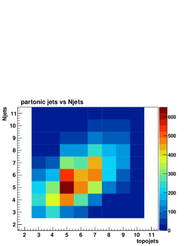
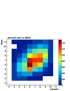
Figure 2: Inclusive number of jets vs expected number of partonic colored particles from topological considerations. In the left, center and right plot scenarios of type A, B and C are shown. Cuts for detector level jets are $p_{T}>50$ GeV and $|\eta|<2.5$.

At detector level in a fully hadronic LHC event, it is clear that we are not able to directly observe the number of SUSY decay products. However, this number should be correlated to the number of observed jets in the detector, even after taking into account the effects of initial and final state radiation, underlying event, hadronization and detector acceptances. In Fig. 2, we show this correlation between the number of SUSY decay products and the number of observed jets in the detector. Keep in mind, that we only take account of jets satisfying $p_{T}>50$ GeV and $|\eta|<2.5$. As can be seen from there, this correspondence is significantly smeared out by all the undesired radiation, hadronization and detector effects, but it is nevertheless still visible. This observation enables us to propose the following two criteria for the separation of the two different edges:

• bino edge:  4-5 jets & lepton veto,

• wino edge:  $\geq$ 6 jets & 1 lepton.

These are the basis of the semi-inclusive jet multiplicity endpoint selection. For the bino selection, we opt for 4-5 jet bins rather than selecting $\leq$4 jets events. In the 4-5 jets events, wino contamination is slightly larger than in the $\leq$4 jets events. However, the $\leq$4 jets events generally suffer from rather large Standard Model backgrounds and a small signal cross section (see Fig. 2). On the other hand, some level of wino contamination is acceptable in the bino edge measurement, because the bino endpoint is larger than the wino endpoint, and the wino contamination is naturally suppressed at the vicinity of the bino endpoint. For the wino selection, instead of taking a $\geq$ 8 jets sample we select $\geq$ 6 jets + 1 lepton. By lepton we mean either an electron or a muon with $p_{T}>20$ GeV and $|\eta|<2.5$. This is due to a leptonically decaying $W$, with which we are able to decrease the overall number of jets in the event by two (see Eq. (2)) and thus drastically reduce the number of wrong jet parings.

However, we should keep in mind that the correlation shown in Fig. 2 is not too strong. The restriction to a maximum of four or five jets thus kills a lot of the wino contamination, but the ratio $N(\tilde{B})/N(\tilde{W})$ of bino to wino events still remains in the ballpark of $0.3-0.7$, depending upon the spectrum. Extending the number of jets up to five is indispensable for types B and C since it increases the statistics at the prize of a slightly reduced sample purity, i.e. ratio of bino to wino events. The relative ratio of wino to bino events in the wino selection is a lot better than in the bino case: $N(\tilde{W})/N(\tilde{B})\sim\mathcal{O}(10)$.

After defining the two relevant selection criteria, we are able to discuss the corresponding SM background contributions in more detail. The dominant processes after the bino endpoint selection are QCD multijet production, where $E_{T}^{\rm miss}$ originates from neutrinos produced in heavy flavor quark decays and jet energy mismeasurements due to instrumental effects, and the production of neutrino pairs from $Z$ boson decays in association with hard jets ($Z$+jets). The production of leptonically decaying $t\bar{t}$ pairs and leptonically decaying $W$ bosons in association with hard jets ($W$+jets) is expected to be suppressed by the lepton veto. To further reduce the background a cut on $Y_{MET}=E_{T}^{\rm miss}/\sqrt{H_{T}}$, which is used in SUSY searches at ATLAS and CMS [25, 26], can be introduced in addition.

In contrast to the bino selection the wino endpoint selection criteria are expected to suppress the SM background in a way that allows to extract endpoints without applying further cuts. By requiring one lepton on top of the baseline selection mentioned above the background from QCD multijet production is anticipated to be completely suppressed. By selecting events with at least six hard jets most of $W$+jets and $Z$+jets events are also expected to be rejected.

4 Kinematic variables for endpoint extraction

Our semi-inclusive jet samples contain 4 or 5 jets for the bino selection and $\geq$ 6 for the wino selection, and we should therefore determine how to select gluino dijets out of a large number of possible jet pairings. In the event samples there are many jets that are not originating from the gluino three body decay. Those are mainly coming from ISR as well as from the $W$ decay. In the scenarios A and B, an additional jet comes from the squark decay, too. It can be argued that the gluino dijets have relatively high $p_{T}$ compared to the ISR and $W$ decay products, which as a kinematical effect is easy to understand.

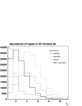
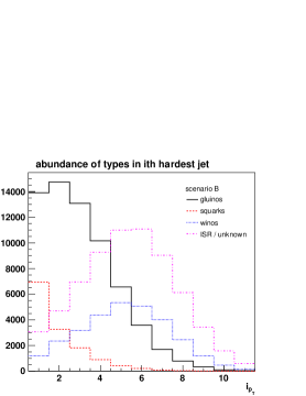
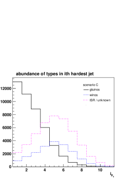
Figure 3: Abundances of gluino (black full line), squark (red dashed line), wino (blue full line) and ISR/unknown jets (blue dotted line) are shown in an inclusive sample for jet bins of hardness $i$ in scenarios A, B and C from left to right.

Figure 3 shows the abundance of gluino, squark and wino jets in $i$-th hardest jet, sorted by $p_{T}$, for the three benchmark scenarios. The identification is done using MC truth by matching detector level jets to partonic objects. Objects, which are not successfully assigned to originate from SUSY mothers are thus either from ISR or other clustering effects of the jet algorithm. As can be seen, for scenarios A, B and C, the first three $p_{T}$-hardest jets are most likely coming from the gluino decay. However for scenarios A and B, there is a significant contribution in the highest $p_{T}$ jet bin from the squark decay $\tilde{q}\to j\tilde{B}\,(\tilde{W})$. If the squark jet is wrongly selected and contributes to the distribution, there is a high risk to exceed the correct gluino endpoint because the dijet mass tends to be large because of the large $p_{T}$ of the squark jet. This is the motivation for the minimization procedure introduced in the following variables, which takes care of this:

$$min_{3j} = \min_{k=1,2}\{m_{3k}\}$$ (3)

$$min_{123} = \min_{i,j=1,2,3}\{m_{ij}\},\qquad i\neq j$$ (4)

Here $m_{ij}$ denotes the invariant mass of jets $i$ and $j$. The endpoint of $min_{3j}$ is expected to be the same as the gluino endpoint as long as one of the first two highest $p_{T}$ jets and the third highest $p_{T}$ jet are coming from the same gluino decay. The $min_{123}$ is smaller than $min_{3j}$ event-by-event because of the wider range of the minimization and has the same endpoints as the gluino’s as long as two of the first three highest $p_{T}$ jets are coming from the same gluino decay. In scenario A, the relative abundance of gluino jets does not look very promising. However keeping in mind, that most of the time we are left with only one gluino, the two variables proposed above we expect to also work reasonably well.

In scenario B, it is reasonable to explicitly exclude the highest $p_{T}$ jet bin and build a distribution out of the remaining three hardest jets, since the gluino jets have the highest relative abundance in these bins. This is the motivation behind the following variable:

$$min_{234}=\min_{i,j=2,3,4}\{m_{ij}\},\qquad i\neq j$$ (5)

Here we explicitly remove the highest $p_{T}$ jet and select the dijet pair among the second, third and fourth highest jets, which yields the smallest invariant mass. This variable should have the same endpoint as the gluino if two of those jets are being originated from the same gluino decay.

There exist other methods in the literature, which address parts of this particular problem of combinatorics in gluino endpoint extraction. Two prominent examples are the hemisphere method [16] as well as a topological method for 4 jets + $\not{E}_{T}$ proposed in [9]. We give a brief overview over both these methods as we compare them to our kinematical variables.

In the hemisphere method, every event is divided into two hemispheres defined by two seeds. These are usually taken to be the hardest object in the event and the one that maximizes the variable $\Delta R\cdot p$, with $\Delta R=\sqrt{\Delta\eta^{2}+\Delta\phi^{2}}$. Then all objects are subsequently clustered to one of the two spatial areas, defined by the seeds. This is done by assigning each particle to that hemisphere which minimizes the value of the Lund distance measure,

$$d(p_{k},p^{(s)}_{j})=(E_{j}-p^{(s)}_{j}\cos\theta_{jk})\frac{E_{j}}{(E_{j}+E_{k})^{2}}$$ (6)

between the four momentum $p_{k}$ of the object to be associated and the two seed momenta $p^{(s)}_{1}$ and $p^{(s)}_{2}$. After all objects are clustered, the seeds are updated to be the sum of all objects in the corresponding hemisphere. Finally, the procedure is iterated until the assignment converges (more details on the specifics of this algorithm can be found in [16]). Once two hemispheres are obtained, we pick up the first two highest $p_{T}$ jets from one of the two hemispheres, which defines the following two variables:

$$m^{(1)}_{12}=m_{12}\leavevmode\nobreak\ \leavevmode\nobreak\ ({\rm from\leavevmode\nobreak\ hemisphere\leavevmode\nobreak\ 1}),\leavevmode\nobreak\ \leavevmode\nobreak\ \leavevmode\nobreak\ \leavevmode\nobreak\ m^{(2)}_{12}=m_{12}\leavevmode\nobreak\ \leavevmode\nobreak\ (\rm from\leavevmode\nobreak\ hemisphere\leavevmode\nobreak\ 2),$$ (7)

where hemisphere 1 is defined as the hemisphere which contains the highest $p_{T}$ jet in the event.

Concerning the second method, in ref. [9], the authors have studied the possibility of identifying the dominant event topology in exclusive 4 jet + $\not{E}_{T}$ events. For this purpose, they defined two dijet mass variables, $F_{3}$ and $F_{4}$. $F_{3}$ is designed for event topologies where 3 jets come from the same cascade chain and 1 jet from the other one. It is given by

$$F_{3}(p_{1},p_{2},p_{3},p_{4})=m_{kl},\qquad\text{ for}\quad\epsilon_{ijkl}\neq 0\quad\text{and}\quad m_{ij}=\max_{r,s=1,\dots,4}\{m_{rs}\}$$ (8)

which is the invariant dijet mass opposite to the maximum of all possible dijet masses. This variable has the same endpoint as the largest dijet mass endpoint originating from the cascade chain producing the 3 jets. $F_{4}$ is, in contrast, designed for the symmetric event topology where both the cascade chains produce 2 jets each. The definition of this variable is given by

$$F_{4}(p_{1},p_{2},p_{3},p_{4})=\min_{i,j=1,\dots,4}\{\max\left(m_{ij},m_{kl}\right)\},\qquad\epsilon_{ijkl}\neq 0.$$ (9)

which is the minimum of the larger dijet mass pair out of three possible combinations. It has the same endpoint as the dijets coming from the same cascade chain each. Although those variables have originally been defined to address exclusive 4 jet + $\not{E}_{T}$ events, we use them for our bino and wino selection samples by applying them to just the first four highest $p_{T}$ jets.

5 Disentangling gluino endpoints

In this section, we show the distributions of the variables defined in the previous section. We assume LHC at 14 TeV with an integrated luminosity of 300 fb$\mbox{}^{-1}$, which corresponds to 108k, 27.6k, and 16.2k signal events for scenarios of type A, B and C, respectively, according to the leading order cross section computed by Herwig++. Notice, that these numbers are conservative in that SUSY QCD NLO corrections for squark and gluino production are known to increase cross sections by a K-factor of up to 2 [19]. In the simulation we take account of all the QCD productions, possible decays, and the effects of parton showering, hadronization and detector simulation.

5.1 Scenario A

bino                                                          wino

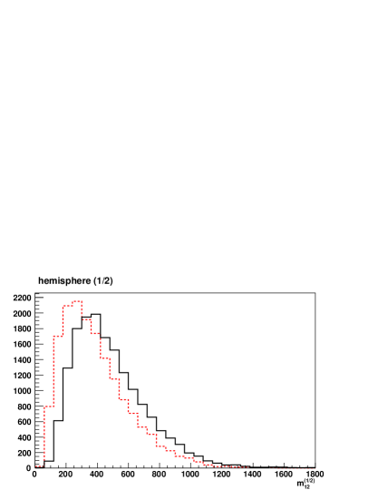
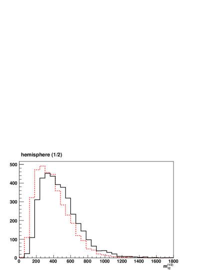
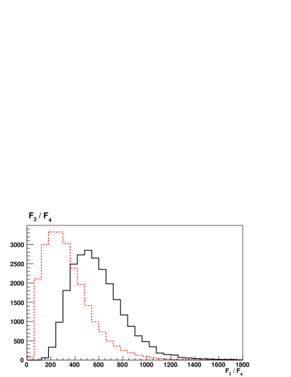
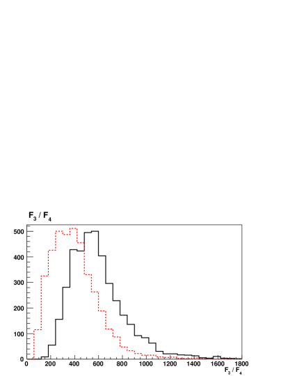
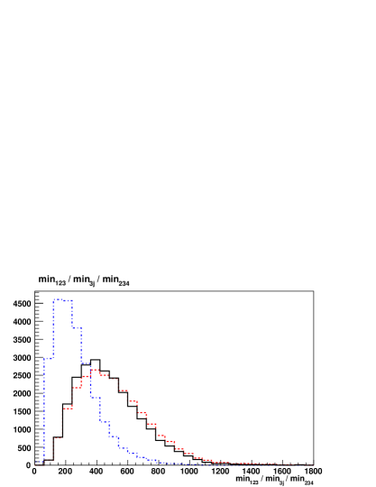
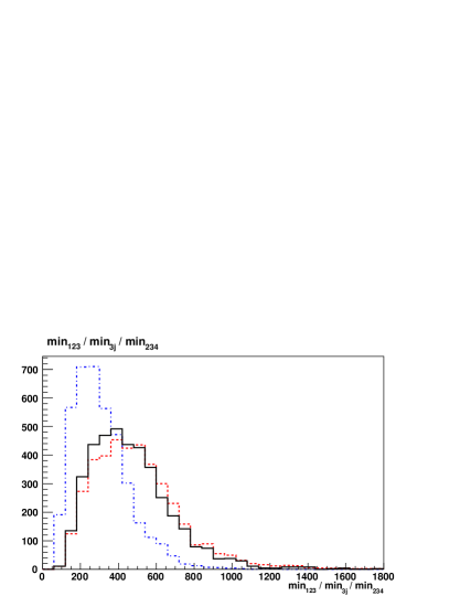
Figure 4: Scenario A: first row: invariant mass of two hardest objects $m_{12}^{(1)}$ and $m_{12}^{(2)}$ for hemispheres 1 (solid, black) and 2 (dashed,red). Second row: $F4$ (solid, black) and $F3$ (dashed,red). Third Row: $min_{123}$ (solid, black), $min_{3j}$ (dashed,red) and $min_{234}$ (dot-dashed, blue). All variables are defined in section 4. The left and right column correspond to the bino and wino selection criteria, respectively.

In scenario A, the mass splitting between squark and gluino is only 100 GeV. The associated $\tilde{q}\tilde{g}$ process dominates the SUSY production. The squarks decay preferably into bino or wino directly because the decay mode into gluino is kinematically suppressed. This reduces the number of signal gluinos from two to one compared to the other scenarios. The ‘squark jet’ coming from $\tilde{q}\to j\tilde{B}\,(\tilde{W})$ has a significant $p_{T}$ (c.f. Fig. 3) and it should be avoided in favorable dijet combinations, either by minimization or explicit removal for example in the construction of $min_{234}$.

Fig. 4 shows the distributions of the various variables discussed in the previous section for the scenario A. In the left (right) row, the bino (wino) event selection (4 or 5 jets for bino, $\geq$ 6 jets & $\geq$ 1 lepton for wino) is applied. In the two plots on the top, the dijet is chosen as the first two highest $p_{T}$ jets in one of the two hemisphere groups. The black solid histograms consider the hemisphere 1, which contains the highest $p_{T}$ in the event and the red dashed histograms consider the other hemisphere group (hemisphere 2). In the middle line, the black solid histograms show $F_{4}$ and the red dashed represent $F_{3}$. The bottom plots show $min_{123}$ (black solid), $min_{3j}$ (red dashed) and $min_{234}$ (blue dot-dashed).

For the bino edge measurement, $F_{3}$ and $F_{4}$ fail to recover the correct edges. $min_{123}$ and $min_{3j}$ have very similar distributions, but nonetheless both have a slight tendency to overshoot the correct endpoint. The hemisphere variables $m_{12}^{(1)}$ and $m_{12}^{(2)}$ also have endpoint structures around the true bino edge. Especially $m_{12}^{(2)}$ from the softer hemisphere looks most promising out of the examined variables. This is expected due to typically only one gluino and the asymmetric nature of the signal in scenario A.

For the wino edge measurement, most of the distributions have tails above the correct value. These tails are bigger for $min_{123}$ and $min_{3j}$ and a kink structure is less pronounced. However, both $m_{12}^{(2)}$ and $F_{3}$ show a nice edge structure at the vicinity of the true endpoint.

5.2 Scenario B

bino                                                          wino

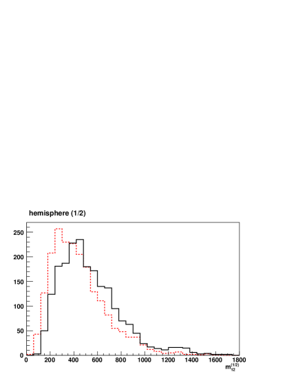
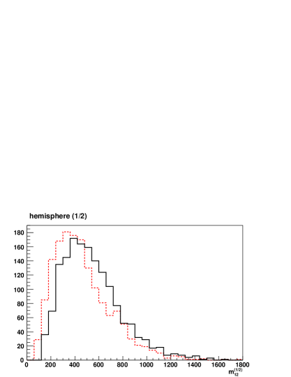
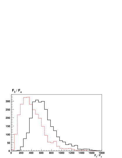
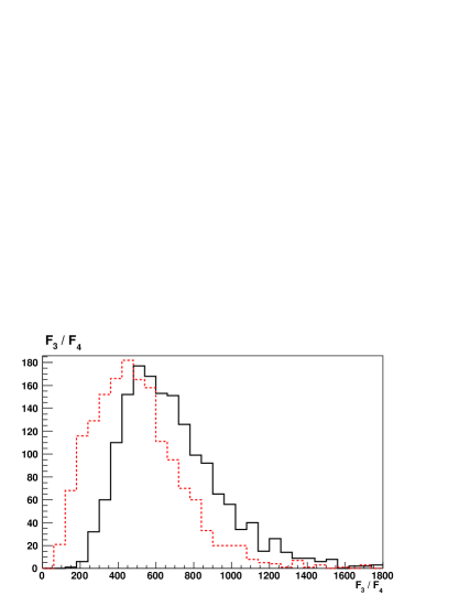
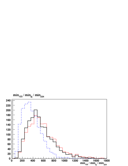
Figure 5: Scenario B: performance of the variables under investigation. For details, see description of Fig.4.

In the type B spectrum, the squark is marginally heavier than in scenario A and the associated $\tilde{q}\tilde{g}$ production still has a sizable cross section compared to the $\tilde{g}\tilde{g}$ process. The main squark decay mode is $\tilde{q}\to j\tilde{g}$. As this ‘squark jet’ has a large $p_{T}$ compared to the other jets (c.f. Fig. 3), it is quite problematic because it is likely to be in the first three highest $p_{T}$ jets and thus increases the number of wrong jet pairings.

Fig. 5 shows the distributions of the variables in scenario B. It is obvious that many of the distributions get shifted to higher mass regions and overshoot the true endpoint. For the bino edge measurement, the $m_{12}^{(1)}$ and $m_{12}^{(2)}$ variables obtained from the hemisphere method work quite well. The $F_{4}$ variable significantly overshoots the true endpoint, while $F_{3}$ seems to recover the gluino endpoint, although the slope around the endpoint is quite shallow. The distributions of $min_{123}$ and $min_{3j}$ are again very similar. They exhibit a long tail above the gluino mass edge but some structure seems still visible at the vicinity of the true endpoint.

For the wino edge measurement, most of the variables fail to recover the correct endpoint. $min_{234}$ on the other hand has a structure around the true wino edge. A good behaviour for $min_{234}$ is expected in scenario B, since the highest $p_{T}$ jet bin has a dangerous contamination from the squark jet, and gluino jets are more safely to be picked up from the second, third and fourth highest $p_{T}$ jets (cf. Fig. 3 or section 4).

5.3 Scenario C

bino                                                          wino

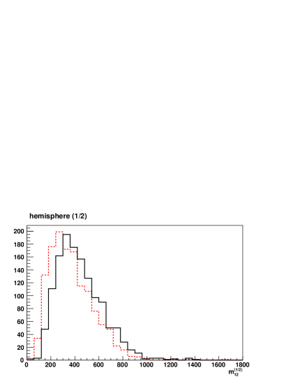
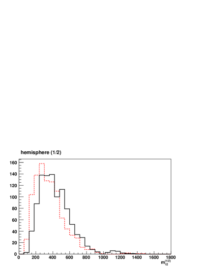
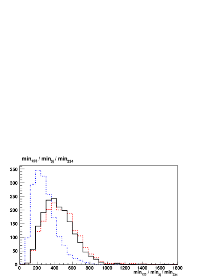
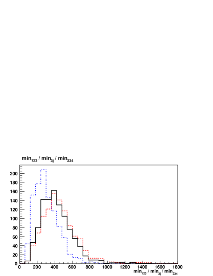
Figure 6: Scenario C: performance of the variables under investigation. For details, see description of Fig.4.

In the type C scenario, decoupled squarks with masses of 10 TeV are not accessible at the LHC energy and the $\tilde{g}\tilde{g}$ production is the unique SUSY QCD production. Many studies regarding combinatorial issues are based on this type of spectrum, and most of them consider only one particular gluino decay mode: $\tilde{g}\to jj\tilde{B}$.

In Fig. 6, we show the results for this spectrum. As can be seen, almost all variables successfully recover the wino edge at 800 GeV. For the bino event selection, most variables suffer from poor statistics in the vicinity of the true endpoint, 1000 GeV. It seems $F_{4}$, $min_{123}$ and $min_{3j}$ perform quite well since their distribution linearly fall down to the true endpoint.

6 Endpoint determination

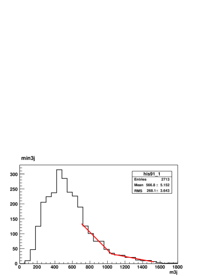
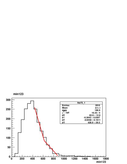
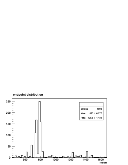
Figure 7: Examples of bino and wino selection in scenario B and C, respectively: we use the edge-to-bump method to obtain a naive endpoint distribution of the variables $min_{3j}$ (bino, first row) and $min_{123}$ (wino, second row).

We attempt to estimate the endpoints of the distributions quantitatively by adopting the edge-to-bump method proposed in [27]. In that method, “kinky” features of distributions which could be originating from an underlying kinematic feature of the distribution or simply be artifacts of statistical fluctuations as well as trigger and cut effects distorting originally smoother distributions, are turned into bumps. Bumps are far easier accessible to data analysis methods, and it is easier to define a systematic error on the procedure of edge determination as this is translated to a statistical error of pseudo-experiments with different edge-to-bump conversion parameters. Roughly speaking, the edge-to-bump method fits the changes in the slopes of the distributions and translates them into peaks. The more distinct a peak is, the more likely it is that there is a true kinematic kink in the original distribution. In this method, for that purpose a naive linear kink fit is used. The resulting value of the fit usually suffers from a non-negligible correlation to the fitting range set by hand. To minimize this artifact, we carry out 1000 naive kink fits with randomly generated fitting ranges and obtain a statistical distribution of endpoint positions.

Fig. 7 shows two examples of endpoint distributions. They are obtained by fitting two different distributions for the bino and wino selection in scenario B and C. As we can see, the peak of the distribution is strongly correlated with the theoretically expected endpoint.

As a first estimate one might give the mean value and the corresponding standard deviation as associated error. However, smaller peaks and non-negligible contributions far off the main peak lead to shifted mean values and considerably large errors ($\mathcal{O}(300)$ GeV). Thus to quantitatively estimate the actual endpoint position and get rid of the contributions far away from the main peak, we apply the following procedure:

endpt.	$min_{123}$	$min_{234}$	$min_{3j}$	$m_{12}^{(1)}$	$m_{12}^{(2)}$	$F_{3}$	$F4$
scenario A
bino	1106 $\pm$ 52	570 $\pm$ 14	1125 $\pm$ 106	822 $\pm$ 21	1012 $\pm$ 104	686 $\pm$ 33	1191 $\pm$ 132
wino	908 $\pm$ 83	665 $\pm$ 34	948 $\pm$ 99	932 $\pm$ 31	780 $\pm$ 26	794 $\pm$ 33	1031 $\pm$ 53
scenario B
bino	986 $\pm$ 36	773 $\pm$ 147	1028 $\pm$ 34	1010 $\pm$ 6	794 $\pm$ 49	766 $\pm$ 25	1046 $\pm$ 66
wino	895 $\pm$ 23	748 $\pm$ 68	892 $\pm$ 18	958 $\pm$ 10	819 $\pm$ 47	911 $\pm$ 51	928 $\pm$ 37
scenario C
bino	812 $\pm$ 24	545 $\pm$ 8	921 $\pm$ 37	816 $\pm$ 29	721 $\pm$ 90	708 $\pm$ 22	894 $\pm$ 57
wino	778 $\pm$ 23	577 $\pm$ 19	804 $\pm$ 6	769 $\pm$ 47	764 $\pm$ 14	708 $\pm$ 38	793 $\pm$ 7

Table 2: Fit values for the discussed variables in the two endpoint selections, obtained with our own implementation of the edge-to-bump method [27]. The values closest to the true endpoints are highlighted in bold face.

1. calulate the mean value $\hat{m}_{0}$ and standard deviation $\sigma_{0}$ of the complete distribution

2. redefine the range of the distribution according to the above values: $\hat{m}_{0}\pm 2\sigma_{0}$

3. calculate a new mean value $\hat{m}_{i}$ and standard deviation $\sigma_{i}$ inside the range defined above

4. use $\hat{m}_{i}$ and $\sigma_{i}$ as a new seed and start over with point 2

Iterating three to six times the steps 2-4, we find convergence of $\hat{m}_{i}$ and $\sigma_{i}$. The resulting mean values and errors obtained by this procedure are listed in Table 2. A first conclusion is that no variable works perfectly for all scenarios, which suggests that one should carefully choose the variables depending on the mass spectrum and the endpoints (bino or wino) to be measured. In scenario A, $m_{12}^{(2)}$ serves the best estimates of the bino and wino endpoints among all variables. $min_{123}$ and $min_{3j}$ possess shifts of about 100 GeV towards higher mass regions but preserve the correct difference between the wino and bino edges. In scenario B, the $\tilde{q}\tilde{g}$ associated production gives an additional high $p_{T}$ jet and the size of the combinatorial background is the largest among the three scenarios. However, $min_{123}$, $min_{3j}$ and $m_{12}^{(1)}$ ($min_{234}$ and $m_{12}^{(2)}$) provide consistent results with the theoretically expected value for the bino (wino) edge measurement and the errors are somewhat smaller than in scenario A. On the other hand, the difference among the two endpoints are underestimated by most variables. This reflects the importance to use an appropriate variable depending on wether a wino or bino selection criterium is applied. In scenario C, all variables tend to underestimate the bino endpoint, despite the fact that the combinatorial and SUSY backgrounds are smallest in size among the three scenarios. This lower bias effect stems from poor statistics due to a small SUSY cross section in scenario C. We checked that the tendency of underestimation is removed when the number of events is increased artificially. For the wino edge, many variables, $min_{123}$, $min_{3j}$, $m_{12}^{(1)}$, $F_{4}$, give good results with small errors.

Finally we want to stress that the quoted errors in Table 2 are only errors originating from the fitting range dependence on fit results and there exist other sources of errors, which should be taken into account. For example, the statistical error on each bin content and the biases inherent in the according variable as well as backgrounds would all give contributions of the size of the errors we quoted. A careful estimation of these is beyond the scope of this paper but will be an important subject for gluino endpoint measurements.

7 Conclusions

In this work we studied the feasibility of the gluino dijet mass edge measurement in a realistic LHC environment. This includes both full SUSY backgrounds and combinatorical miscombinations of particles, as well as effects of initial and final state radiation and finite detector resolution. Several methods in the literature explicitly rely on the precise knowledge of a particular endpoint to be able to access information on masses in decay cascades, to resolve combinatorial issues, or determine another kinematical variable. Often QCD radiation and detector effects have been neglected in first phenomenological investigations. By utilizing considerations from the analysis of topological configurations of gluino decay cascades at the parton level, we find that the surviving correlation between the number of parton level and detector level jets is sufficient in distinguishing bino and wino endpoints of gluino decays with semi-inclusive jet multiplicities and the use of leptons as further selection criteria. To assess the impact of different mass spectra, we analyse three distinct (semi-)simplified models: two with small and large mass differences between gluino and squarks, and one scenario with decoupled scalars. In these models, we make use of existing kinematic variables and propose new ones, where necessary, that reduce the combinatorical problem and, when applied to preselected events, allow for the excavation of two distinct gluino endpoints. In general, the kinematic variables presented here are robust against contaminations from QCD radiation, underlying (non-signal) SUSY processes as well as detector effects. The resulting distributions are fitted with the so-called edge-to-bump method minimizing the artifact of the fit. These first estimates of the gluino dijet endpoints are mostly consistent with their expected values and thus proof the validity of our method. Hence, it seems possible to measure the gluino dijet edges for basically all cases where the squarks are heavier than the gluino, a parameter space that seems to be favored by recent Higgs search analyses from the LHC experiments.

Acknowledgements

We would like to thank Christian Sander and Matthias Schröder for valuable comments and helpful discussions. JRR and DW like to thank the Institute of Physics of the University of Freiburg for their hospitality.

References

- [1] A. J. Barr and C. G. Lester, J. Phys. G G 37 (2010) 123001 [arXiv:1004.2732 [hep-ph]].
- [2] I. Hinchliffe, F. E. Paige, M. D. Shapiro, J. Soderqvist and W. Yao, Phys. Rev. D 55 (1997) 5520 [hep-ph/9610544]; H. Baer, C. -h. Chen, M. Drees, F. Paige and X. Tata, Phys. Rev. D 59 (1999) 055014 [hep-ph/9809223]; I. Hinchliffe and F. E. Paige, Phys. Rev. D 60 (1999) 095002 [hep-ph/9812233]; H. Bachacou, I. Hinchliffe and F. E. Paige, Phys. Rev. D 62 (2000) 015009 [hep-ph/9907518]; I. Hinchliffe and F. E. Paige, Phys. Rev. D 61 (2000) 095011 [hep-ph/9907519]; B. C. Allanach, C. G. Lester, M. A. Parker and B. R. Webber, JHEP 0009 (2000) 004 [hep-ph/0007009].
- [3] C. G. Lester and D. J. Summers, Phys. Lett. B 463 (1999) 99 [hep-ph/9906349]; A. Barr, C. Lester and P. Stephens, J. Phys. G G 29 (2003) 2343 [hep-ph/0304226]; W. S. Cho, K. Choi, Y. G. Kim and C. B. Park, Phys. Rev. Lett. 100 (2008) 171801 [arXiv:0709.0288 [hep-ph]]; W. S. Cho, K. Choi, Y. G. Kim and C. B. Park, JHEP 0802 (2008) 035 [arXiv:0711.4526 [hep-ph]]; B. Gripaios, JHEP 0802 (2008) 053 [arXiv:0709.2740 [hep-ph]]; A. J. Barr, B. Gripaios and C. G. Lester, JHEP 0802 (2008) 014 [arXiv:0711.4008 [hep-ph]]. M. Burns, K. Kong, K. T. Matchev and M. Park, JHEP 0903 (2009) 143 [arXiv:0810.5576 [hep-ph]]; P. Konar, K. Kong, K. T. Matchev and M. Park, Phys. Rev. Lett. 105 (2010) 051802 [arXiv:0910.3679 [hep-ph]]; T. Cohen, E. Kuflik and K. M. Zurek, JHEP 1011 (2010) 008 [arXiv:1003.2204 [hep-ph]]; A. J. Barr, B. Gripaios and C. G. Lester, JHEP 0911 (2009) 096 [arXiv:0908.3779 [hep-ph]]; P. Konar, K. Kong, K. T. Matchev and M. Park, JHEP 1004 (2010) 086 [arXiv:0911.4126 [hep-ph]].
- [4] C. Lester and A. Barr, JHEP 0712 (2007) 102 [arXiv:0708.1028 [hep-ph]];
- [5] M. M. Nojiri, Y. Shimizu, S. Okada and K. Kawagoe, JHEP 0806 (2008) 035 [arXiv:0802.2412 [hep-ph]]; M. M. Nojiri, K. Sakurai, Y. Shimizu and M. Takeuchi, JHEP 0810 (2008) 100 [arXiv:0808.1094 [hep-ph]]; S. -G. Kim, N. Maekawa, K. I. Nagao, M. M. Nojiri and K. Sakurai, JHEP 0910 (2009) 005 [arXiv:0907.4234 [hep-ph]].
- [6] D. R. Tovey, JHEP 0804 (2008) 034 [arXiv:0802.2879 [hep-ph]]; G. Polesello and D. R. Tovey, JHEP 1003 (2010) 030 [arXiv:0910.0174 [hep-ph]]. G. G. Ross and M. Serna, Phys. Lett. B 665 (2008) 212 [arXiv:0712.0943 [hep-ph]]; A. J. Barr, T. J. Khoo, P. Konar, K. Kong, C. G. Lester, K. T. Matchev and M. Park, Phys. Rev. D 84 (2011) 095031 [arXiv:1105.2977 [hep-ph]]. B. Gripaios, A. Papaefstathiou, K. Sakurai and B. Webber, JHEP 1101 (2011) 156 [arXiv:1010.3962 [hep-ph]]; A. J. Barr, S. T. French, J. A. Frost and C. G. Lester, JHEP 1110 (2011) 080 [arXiv:1106.2322 [hep-ph]]; L. A. Harland-Lang, C. H. Kom, K. Sakurai and W. J. Stirling, Eur. Phys. J. C 72 (2012) 1969 [arXiv:1110.4320 [hep-ph]]; L. A. Harland-Lang, C. H. Kom, K. Sakurai and W. J. Stirling, Phys. Rev. Lett. 108 (2012) 181805 [arXiv:1202.0047 [hep-ph]].
- [7] M. Serna, JHEP 0806 (2008) 004 [arXiv:0804.3344 [hep-ph]]. H. -C. Cheng and Z. Han, JHEP 0812 (2008) 063 [arXiv:0810.5178 [hep-ph]];
- [8] K. Desch, J. Kalinowski, G. A. Moortgat-Pick, M. M. Nojiri and G. Polesello, JHEP 0402 (2004) 035 [hep-ph/0312069]; K. Kawagoe, M. M. Nojiri and G. Polesello, Phys. Rev. D 71 (2005) 035008 [hep-ph/0410160]; H. -C. Cheng, J. F. Gunion, Z. Han, G. Marandella and B. McElrath, JHEP 0712 (2007) 076 [arXiv:0707.0030 [hep-ph]]; H. -C. Cheng, D. Engelhardt, J. F. Gunion, Z. Han and B. McElrath, Phys. Rev. Lett. 100 (2008) 252001 [arXiv:0802.4290 [hep-ph]]; H. -C. Cheng, J. F. Gunion, Z. Han and B. McElrath, Phys. Rev. D 80 (2009) 035020 [arXiv:0905.1344 [hep-ph]]; B. Webber, JHEP 0909 (2009) 124 [arXiv:0907.5307 [hep-ph]]; M. M. Nojiri, K. Sakurai and B. R. Webber, JHEP 1006 (2010) 069 [arXiv:1005.2532 [hep-ph]].
- [9] Y. Bai and H. -C. Cheng, JHEP 1106 (2011) 021 [arXiv:1012.1863 [hep-ph]].
- [10] B. Gripaios, K. Sakurai and B. Webber, JHEP 1109 (2011) 140 [arXiv:1103.3438 [hep-ph]].
- [11] B. Dutta, T. Kamon, N. Kolev and A. Krislock, Phys. Lett. B 703 (2011) 475 [arXiv:1104.2508 [hep-ph]].
- [12] A. Rajaraman and F. Yu, Phys. Lett. B 700 (2011) 126 [arXiv:1009.2751 [hep-ph]]; P. Baringer, K. Kong, M. McCaskey and D. Noonan, JHEP 1110 (2011) 101 [arXiv:1109.1563 [hep-ph]]; K. Choi, D. Guadagnoli and C. B. Park, JHEP 1111 (2011) 117 [arXiv:1109.2201 [hep-ph]];
- [13] J. Alwall, K. Hiramatsu, M. M. Nojiri and Y. Shimizu, Phys. Rev. Lett. 103 (2009) 151802 [arXiv:0905.1201 [hep-ph]].
- [14] M. M. Nojiri and K. Sakurai, Phys. Rev. D 82 (2010) 115026 [arXiv:1008.1813 [hep-ph]].
- [15] K. Hagiwara et al., Phys. Rev. D 73, 055005 (2006) [arXiv:hep-ph/0512260].
- [16] G. L. Bayatian et al. [CMS Collaboration], J. Phys. G G 34 (2007) 995.
- [17] M. Bahr, S. Gieseke, M. A. Gigg, D. Grellscheid, K. Hamilton, O. Latunde-Dada, S. Platzer and P. Richardson et al., Eur. Phys. J. C 58 (2008) 639 [arXiv:0803.0883 [hep-ph]].
- [18] W. Kilian, T. Ohl and J. Reuter, Eur. Phys. J. C 71 (2011) 1742 [arXiv:0708.4233 [hep-ph]]; M. Moretti, T. Ohl and J. Reuter, arXiv:hep-ph/0102195; W. Kilian, J. Reuter, S. Schmidt and D. Wiesler, JHEP 1204, 013 (2012) [arXiv:1112.1039 [hep-ph]].
- [19] W. Beenakker, R. Hopker, M. Spira and P. M. Zerwas, Nucl. Phys. B 492 (1997) 51 [arXiv:hep-ph/9610490].
- [20] S. Ovyn, X. Rouby and V. Lemaitre, arXiv:0903.2225 [hep-ph].
- [21] M. Cacciari, G. P. Salam and G. Soyez, JHEP 0804 (2008) 063 [arXiv:0802.1189 [hep-ph]].
- [22] M. Cacciari, G. P. Salam and G. Soyez, arXiv:1111.6097 [hep-ph].
- [23] M. Cacciari and G. P. Salam, Phys. Lett. B 641 (2006) 57 [hep-ph/0512210].
- [24] S. Chatrchyan et al. [CMS Collaboration], JHEP 1108 (2011) 155 [arXiv:1106.4503 [hep-ex]].
- [25] G. Aad et al. [Atlas Collaboration], JHEP 1111 (2011) 099 [arXiv:1110.2299 [hep-ex]].
- [26] S. Chatrchyan et al. [CMS Collaboration], JHEP 1108 (2011) 156 [arXiv:1107.1870 [hep-ex]].
- [27] D. Curtin, Phys. Rev. D 85 (2012) 075004 [arXiv:1112.1095 [hep-ph]].