Strongly interacting Majorana modes in an array of Josephson junctions

Abstract

An array of superconducting islands with semiconducting nanowires in the right regime provides a macroscopic implementation of Kitaev’s toy model for Majorana wires. We show that a capacitive coupling between adjacent islands leads to an effective interaction between the Majorana modes. We demonstrate that even though strong repulsive interaction eventually drive the system into a Mott insulating state the competition between the (trivial) band-insulator and the (trivial) Mott insulator leads to an interjacent topological insulating state for arbitrary strong interactions.

1 Introduction

Majorana zero modes are fermions which are their own antiparticles. They are believed to exist as effective particles in the middle of the gap of a topological superconductor. The recent interest in Majorana zero modes originates in their non-Abelian exchange statistics [1], which is the basis for potential applications in quantum computation [2]. Based on the theoretical proposal [3] to realize this exotic states in semiconducting nanowires with strong spin-orbit coupling in a magnetic field and in proximity to a conventional (nontopological) superconductor, recent experimental progress has shown signatures of Majorana zero modes in the tunnelling conductance of normal conducting-superconducting [4] and superconducting-normal conducting-superconducting systems [5]. More information and references on the fast developing field can be found in the recent reviews [6].

As the nanowire is one-dimensional interaction effects become important. On the one hand, employing field theoretical methods Gangadharaiah et al. [7] have argued that strong electron-electron interactions generically destroy the topological phase by suppressing the superconducting gap. On the other hand, using a combination of analytical and numerical methods Stoudenmire et al. [8] have shown that repulsive interactions significantly decrease the required Zeeman energy and increase the parameter range for which the topological phase exists. It is believed that the origin of these effects is an interaction driven renormalization of the Zeeman gap [8, 9]. Furthermore, it has been shown that in helical liquids the scattering processes between the constituent fermion bands open gaps which in turn lead to a stabilization of the Majorana states against interactions [10] and that (an odd number of) Majorana zero modes are in fact stable against general interactions [11]. For further studies of the effect of electron-electron interactions on Majorana zero modes in nanowires and two-chain ladders see [12].

Recently, a macroscopic version of the Kitaev chain [13], a toy model for a nanowire supporting noninteracting Majorana modes, has been proposed [14] in a one-dimensional (1D) array of topological superconducting islands. Its advantage over microscopic implementations is that the individual parameters of the effective Hamiltonian can potentially be tuned in situ. Here, we show that additional capacitances between adjacent islands lead to an effective interaction between the low-energy Majorana degrees of freedom. We present the phase diagram of the system which demonstrates that sufficiently strong repulsive interactions will drive the system from the topologically trivial phase into the topological phase supporting Majorana zero modes before eventually leading to a Mott insulating state. We discuss how the parameters of the system can be tuned by changing the gate voltages and exploit this to propose the detection of the different phases and phase boundaries in a tunnelling experiment.

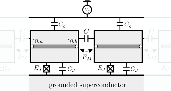
Figure 1: A 1D array of superconducting islands (light grey) coupled via strong Josephson junctions ($E_{J}$) to a common ground superconductor. Each island contains a pair of Majorana zero modes (white dots) at the end points of a semiconducting nanowire (dark grey). The tunnel coupling of individual electrons between the superconducting islands is proportional to the energy scale $E_{M}$. A common gate voltage $V_{g}$ can be used to tune the relative strength of the different terms in the Hamiltonian. The capacitive couplings between the elements are denoted by $C$, $C_{J}$, and $C_{g}$, respectively.

2 Model

We discuss a system consisting of a 1D array of $N$ superconducting islands (see figure 1). Because of the proximity-coupled semiconducting nanowire each of the islands has two midgap Andreev states, i.e., Majorana modes, located at the ends of the nanowire [3]. We will denote with $\gamma_{ka}$ and $\gamma_{kb}$ the two Majorana operators on island $k$ associated with these zero modes. The Majorana operators are Hermitian $\gamma_{\mu}=\gamma_{\mu}^{\dagger}$ and fulfil the Clifford algebra $\{\gamma_{\mu},\gamma_{\nu}\}=2\delta_{\mu\nu}$. The total Lagrangian $L=T-V_{J}-V_{M}$ of the system consists of three terms. Coupling of the Majorana modes on nearby islands leads to the term [13, 15] $V_{M}=i\,E_{M}\sum_{k=1}^{N}\gamma_{kb}\gamma_{k+1a}\cos[(\phi_{k+1}-\phi_{k})/2]$ where $\phi_{k}$ is the superconducting phase of the $k$-th island. Here and in the following, we assume for convenience periodic boundary condition such that islands 1 and $N+1$ are equivalent. Apart from the Majorana modes, the term discussed above has the additional degrees of freedom $\phi_{k}$ due to the condensate of Cooper pairs. Similar to [14], we eliminate these by connecting each superconducting island with a strong Josephson junction to a common (ground) superconductor. This fixes the superconducting phases (up to some quantum phase-slips discussed below) and is described by the Hamiltonian $V_{J}=E_{J}\sum_{k=1}^{N}(1-\cos\phi_{k});$ here, $E_{J}=\hbar I_{c}/2e$ is the effective Josephson coupling of each of the Josephson junctions with critical current $I_{c}$. In the limit $E_{J}\gg E_{M}$ the junctions effectively pin the phases of all superconducting islands to a common value $\phi_{k}\equiv 0$. As a result $V_{M}$ reduces to the pure Majorana coupling

$$H_{M}=i\,E_{M}\sum_{k=1}^{N}\gamma_{kb}\gamma_{k+1a},\qquad(E_{J}\gg E_{M}).$$ (1)

Finally, the kinetic term $T=(\hbar^{2}/8e^{2})\sum_{k=1}^{N}[C(\dot{\phi}_{k+1}-\dot{\phi}_{k})^{2}+C_{G}\dot{\phi}_{k}^{2}]+(\hbar/2e)\sum_{k=1}^{N}q\dot{\phi}_{k}$ occurs due to the capacitive couplings, where $C$ denotes the capacitance between neighbouring islands and $C_{G}=C_{g}+C_{J}$ the (total) capacitance to the ground. Here, $C_{J}$ is the capacitance of the strong Josephson junction and $C_{g}$ the capacitance to a common back gate at voltage $V_{g}$ with respect to the ground superconductor. Apart from the charging energy, the back-gate introduces a term proportional to the induced charge $q=C_{g}V_{g}$ which is tunable with single-electron precision [16] via $V_{g}$ and whose effect will become important later. The typical capacitive energy scale $E_{C}=e^{2}/2C_{\Sigma}$ of a single islands depends on the total capacitance $C_{\Sigma}=2C+C_{G}$.

3 Mapping on an effective spin model

As we have seen the strong coupling to the ground superconductor pins the superconducting phase differences to $\phi_{k}\equiv 0$ and thus changes the energy due to the Majorana modes from $V_{M}$ to $H_{M}$. The effect of the strong coupling to the ground superconductor on the charging energy $T$ is more subtle. We first present the results for $C=0$ before extending them to nonzero $C$: as charge and phase are conjugate variables the pinning of the phases $\phi_{k}$ greatly reduces the effect of charging [14]. An effective charging energy still arises due to quantum phase slips through the junctions. For example, changing $\phi_{k}$ from $0$ to $2\pi$ leads to a charging energy ($E_{J}\gg E_{C}$) [17]

$$H_{Ck}=\Gamma_{\Delta}\cos[\pi(q/e+n_{k})]=\Gamma_{\Delta}\cos(\pi q/e)\mathcal{P}_{k}.$$ (2)

Here, the tunnelling amplitude is given by $\Gamma_{\Delta}\simeq E_{C}^{1/4}E_{J}^{3/4}e^{-S_{\Delta}}$ with $S_{\Delta}=\hbar^{-1}\int\!d\tau\,L_{E}=\sqrt{8E_{J}/E_{C}}$ the dimensionless Euclidean action along the classical trajectory $\gamma_{\Delta}\colon\phi_{k}\in[0,2\pi]$ in the inverted potential with $L_{E}(\tau)=-L(t=i\tau)$. The cosine term in (2) occurs due to the Aharonov-Casher interference of the two tunnelling paths $\phi_{k}=0\to 2\pi$ and $\phi_{k}=0\to-2\pi$ which lead to an indistinguishable final state and thus interfere with a phase difference depending on the total induced charge $q+en_{k}$ [18, 14]. The term $n_{k}=\frac{1}{2}(1-\mathcal{P}_{k})\in\{0,1\}$ is the contribution to the charge due to the parity $\mathcal{P}_{k}=i\gamma_{ka}\gamma_{kb}\in\{-1,1\}$ of the number of electrons on the superconducting island encoded in the state of the Majorana zero modes [15, 14]. Equation (2) is a chemical potential term: For large $\Gamma_{\Delta}$, all the fermionic states are either filled or empty and the system is in a band insulating state.

Going away from this special point and introducing a finite cross-capacitance parametrized by $\eta=2C/C_{\Sigma}$ with $\eta\in[0,1]$, the classical path for a phase slip in $\phi_{k}$ does not only involve $\phi_{k}$ but also the other phases. To lowest nonvanishing order in $\eta$, we only need to take into account the change in $\phi_{k-1}$ and $\phi_{k+1}$ and obtain $S_{\Delta}=\sqrt{8E_{J}/E_{C}}[1+(\pi^{2}-12)\eta^{2}/96]$, which is accurate to more than 2 digits all the way up to $\eta=1$ as numerics confirms. Additionally, the effective capacitance coupling between two islands becomes important. This term is generated by simultaneous phase slips of the two phases $\phi_{k}$ and $\phi_{k+1}$ of neighbouring islands. Due to the symmetry between island $k$ and $k+1$, we have $\phi_{k}=\phi_{k+1}$ for the classical path $\gamma_{U}\colon\phi_{k}=\phi_{k+1}\in[0,2\pi]$ with the corresponding Euclidean action $S_{U}=\sqrt{16(2-\eta)E_{J}/E_{C}}$. The Aharonov-Casher interference in this case leads to the tunnelling amplitude $\Gamma_{U}\simeq E_{C}^{1/4}E_{J}^{3/4}e^{-S_{U}}$ depending on the total charge $2q+e(n_{k}+n_{k+1})$ of the two islands involved. Thus we obtain the interaction term

$$H_{Uk}=\Gamma_{U}\cos[2\pi q/e+\pi(n_{k}+n_{k+1})]=\Gamma_{U}\cos(2\pi q/e)\mathcal{P}_{k}\mathcal{P}_{k+1}.$$ (3)

We stress that (3) is an interaction term involving four Majorana operators and that the amplitude is modulated by twice the induced charge $q$ compared to (2). We call $U>0$ repulsive interaction as it prefers having an occupied site next to an empty one. For strong repulsive interactions the system is driven into a Mott insulator or equivalently commensurate charge density wave (CDW) state.

The complete low-energy Hamiltonian in the limit $E_{J}\gg E_{M},E_{C}$ is given by $H_{\scriptscriptstyle\rm ANNNI}=\sum_{k=1}^{N}(H_{Ck}+H_{Uk})+H_{M}$, which constitutes the transverse axial next-nearest-neighbour Ising (ANNNI) model [19] as can be seen by performing a Jordan-Wigner transformation $\mathcal{P}_{k}=i\gamma_{ka}\gamma_{kb}=\sigma^{z}_{k}$, $i\gamma_{kb}\gamma_{k+1a}=\sigma^{x}_{k}\sigma^{x}_{k+1}$, resulting in the spin Hamiltonian

$$H_{\scriptscriptstyle\rm ANNNI}=\sum_{k=1}^{N}(\Delta\sigma^{z}_{k}+U\sigma^{z}_{k}\sigma^{z}_{k+1}+E_{M}\sigma^{x}_{k}\sigma^{x}_{k+1}).$$ (4)

Here, the $\sigma_{k}^{x,y,z}$ are Pauli matrices, $\Delta=\Gamma_{\Delta}\cos(\pi q/e)$ and $U=\Gamma_{U}\cos(2\pi q/e)$. We note that the energies $\Delta$ and $U$ can be tuned via the charge $q$ induced on the superconducting islands through the gate voltage $V_{g}$. As the fermionic Hamiltonian without the interaction term proportional to $U$ has been intensively studied before [13], we focus here on the effects of the interaction term. In our set-up, this term is most important in the case $C\gg C_{G}$ where $\eta\approx 1$ and $\Gamma_{U}\approx\Gamma_{\Delta}\exp[-1.25\sqrt{E_{J}/E_{C}}]$, which can be as large as $0.3$ for $E_{J}\approx E_{C}$; note that in this regime the actions $S_{\Delta}$ and $S_{U}$ are still much larger than one such that the semiclassical approximation employed above is valid.

4 Phase diagram

We first note that the system (4) is invariant under $E_{M}\to-E_{M}$ as well as $\Delta\to-\Delta$ due to the transformations $\sigma_{k}^{x,y}\to(-1)^{k}\sigma_{k}^{x,y}$ and $\sigma_{k}^{x,z}\to-\sigma_{k}^{x,z}$ respectively. Thus without loss of generality, we assume in the following $E_{M},\Delta>0$. The phase diagram of the spin model (4) contains four phases: A paramagnetic phase (PM) with a unique ground state with $\langle\sigma_{k}^{z}\rangle<0$, $\langle\sigma_{k}^{x}\rangle=0$; an antiferromagnetic phase (AFM) with doubly degenerate ground state and $\langle\sigma_{k}^{x}\rangle\propto(-1)^{k}$; an “anti phase” (AP) with a doubly degenerate ground state with $\langle\sigma_{k}^{z}\rangle\propto(-1)^{k}$; and a “floating phase” (FP) between the AFM and the AP. For $\Delta=0$, the duality transform of the model (4) is a sum of two quantum Ising chains, while for the noninteracting case it reduces to a single quantum Ising chain.

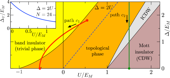
Figure 2: Phase diagram of the Josephson junction array (4). The phase diagram is invariant under $\Delta\to-\Delta$. The topological phase is characterized by a doubly degenerate ground state. In figure 3 we show the tunnelling conductance along the paths $c_{1}$ and $c_{2}$. Inset: Gap $\Delta_{T}$ between the (nearly) degenerate ground states ($\delta\lesssim 0.02\,E_{M}$) and the first excited state along the blue dashed line as determined by exact diagonalization.

As we have shown above in our realization of the ANNNI model the parameters $\Delta$ and $U$ can easily be tuned via a gate voltage. On the other hand, the coupling $E_{M}$ is determined by the overlaps of the Majorana wave functions on neighbouring islands and thus fixed by the geometry of the array. Hence it is natural to consider the phase diagram as function of $\Delta/E_{M}$ and $U/E_{M}$, which is shown in figure 2. For fixed $\Delta/E_{M}>1$ and sufficiently small interaction $U$ the system is in a trivial (band-insulating) phase corresponding to the PM in the effective spin model, which is characterized by an unique ground state with $\langle\mathcal{P}_{k}\rangle<0$. By increasing $U$ we cross into a topological phase (corresponding to the AFM) with $\langle\mathcal{P}_{k}\rangle=0$ and two degenerate ground states $|\pm\rangle$, distinguished by the (total) fermion parity $\prod_{k}\mathcal{P}_{k}|\pm\rangle=\pm|\pm\rangle$. The parity protection (also called topological protection) originates from the fact that any fermionic perturbation conserves the fermion parity and thus cannot mix the states $|\pm\rangle$. The phase transition between the trivial and topological phase is, for $U>0$, located at

$$1-\frac{2U}{\Delta}=\frac{E_{M}}{\Delta}-\frac{UE_{M}^{2}}{2\Delta^{2}(\Delta-U)},\quad\frac{E_{M}}{\Delta}\ll 1.$$ (5)

In particular, we find $\Delta=2U$ for $U\gg E_{M}$. On the other hand, for $|U|\ll E_{M}$ perturbation theory yields $\Delta=E_{M}+32\,U/(6\pi)$.

At large positive $U$ we eventually enter incommensurate and commensurate CDW (Mott insulator) states corresponding to the FP and the AP, respectively. This region of the phase diagram cannot be reached as long as the induced charge $q$ on the islands is homogeneous. However, replacing the common back gate by individual gates for each island yields the model (4) with site-dependent parameters $\Delta_{i}=\Gamma_{\Delta}\cos(\pi q_{i}/e)$ and $U_{i}=\Gamma_{U}\cos(\pi(q_{i}+q_{i+1})/e)$ where $q_{i}=G_{g}V_{g}^{i}$ denotes the induced charge on island $i$. Now using $q_{i}=(-1)^{i}q$ one can enter the Mott phase for $q\to e/2$. Note that the two degenerate ground states in the Mott insulator phase have the same fermion parity and thus are not parity protected.

The main feature of the phase diagram is its strong anisotropy under $U\to-U$. While negative interactions suppress the topological phase, for $U>0$ the ordering tendencies of the first and second term in (4) compete with each other. In particular, starting from a noninteracting point in the trivial phase, i.e., $U=0$ and $\Delta>E_{M}$, competition between the band- and the Mott-insulator will drive the system into the topological phase irrespective of the value of $\Delta/E_{M}$.

As discussed above the topological phase is characterized by the existence of a doubly degenerate ground state with different fermion parity. In a finite system this degeneracy is lifted and the value of the resulting gap $\delta$ depends on the number of islands $N$ as well as the system parameters $\Delta/E_{M}$ and $U/E_{M}$. On the other hand, the existence of Majorana end modes is protected by the gap between the (nearly) degenerate ground states and the first excited state, which we denote by $\Delta_{T}$. This gap is given by $\Delta_{T}=4E_{M}$ at $\Delta=U=0$ and decreases when going away from this point. However, as we show in the inset in figure 2, it remains of the order of $E_{M}$ and significantly larger than $\delta$ for $U\neq 0$ as long as one stays away from the phase boundaries.

5 Tunnelling conductance

After presenting the phase diagram, we now turn to its experimental signatures in the tunnelling conductance. The parameters $\Delta$ and $U$ can be directly tuned through the induced charge $q$ on the islands via a common back gate voltage $V_{g}$ making it possible to choose the parameters such that the path crosses one or more phase boundaries.

Specifically, we consider the path $c_{1}(q)=(\Gamma_{U}\,\cos(2\pi q/e),\Gamma_{\Delta}\,\cos(\pi q/e))$ with $\Gamma_{U}=0.3\,\Gamma_{\Delta}=0.54\,E_{M}$ such that the starting and end points at $q=0$ and $q=e/2$ lie in the topological phase while the path enters the trivial phase in between (see the red curve in figure 2). In the following we consider an open chain of $N$ islands. Following [20], we couple the system to an electronic lead with the tunnel Hamiltonian $H_{T}=t\gamma_{1a}\sum_{k\sigma}(c_{k\sigma}-c^{\dagger}_{k\sigma})$, where $c_{k\sigma}$ are the annihilation operators of the electrons in the lead and $t$ is the tunnelling amplitude. We assume a constant density of states $\rho_{0}$ in the lead such that the (bare) tunnelling probability is given by $\Gamma_{0}=2\pi t^{2}\rho_{0}$. We have calculated the differential Andreev conductance $G(V)$ using exact diagonalization for an open chain of length $N=24$ taking only the two lowest energy states (with different fermion parity) into account. In figure 3(a), the broadened conductance

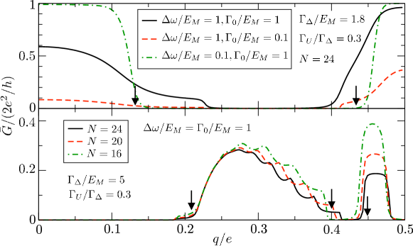
Figure 3: Tunnelling conductance along the paths (a) $c_{1}$ and (b) $c_{2}$ shown in figure 2. The arrows indicate the approximate phase boundaries.

$$\bar{G}=\int_{-\Delta\omega/2}^{\Delta\omega/2}\frac{d(eV)}{\Delta\omega}G(V)$$ (6)

is plotted along $c_{1}$; the broadening $\Delta\omega\simeq\max(eV,k_{B}T)$ is given by the maximum of bias voltage $V$ and temperature $T$. For strong coupling $\Gamma_{0}$ to the lead as well as small broadening $\Delta\omega$, the phase boundaries are clearly visible as points where the conductance jumps from one to zero and vice versa. Weaker coupling to the lead will lead to a suppression of the conductance in the topological phase, i.e., unitary conductance cannot be observed. On the other hand, a larger broadening will eventually smear out all transitions. Thus in order to enable an experimental detection of the phase boundaries the energy broadening should be small (in units of $E_{M}$) while the coupling to the lead has to be sufficiently strong. Recent experiments on proximity coupled nanowires [4] indicate that a Majorana coupling $E_{M}/k_{B}\simeq 100\,$mK is realistic, which is well in the range of experimental accessible temperatures. The Majorana coupling sets the topological gap $\Delta_{T}$ (see inset of figure 2) as the other couplings ($E_{J}$ and $E_{C}$) can be designed in a large parameter range [21].

In order to study the regime of strong interactions we use the set-up with individual back gates and induced charges $q_{i}=(-1)^{i}q$. In this set-up we consider the path $c_{2}(q)=(\Gamma_{U},\Gamma_{\Delta}\,\cos(\pi q/e))$ with $\Gamma_{U}=0.3\,\Gamma_{\Delta}=1.5\,E_{M}$ (see the green curve in figure 2). The conductance $\bar{G}$ along $c_{2}$ is shown in figure 3(b). At $q=0$ the path starts deep in the band insulator phase and enters the topological phase at $q\approx 0.2$ where the conductance becomes nonzero. When further increasing $q$ we observe weak oscillations which are due to the finite size lifting $\delta$ of the ground state degeneracy. For larger values of $q$ the conductance stays zero in the incommensurate and commensurate CDW phases with the exception of the phase transition between them, where the conductance is nonzero due to finite-size effects.

Above we have shown how to realize the 1D ANNNI model using Josephson junction arrays and how to map out its phase diagram by measuring the tunnelling conductance. In this sense our proposed set-up constitutes a quantum simulator for the 1D ANNNI model. In particular, the experimental control over the system parameters like the gate voltages allows to study the effects of disorder on the phase diagram.

6 Relation to nanowires

Interacting electrons in proximity-coupled semiconducting nanowires are described by the microscopic Hamiltonian [8]

$$H_{\rm\scriptsize NW} =-\int\!dx\,\Psi^{\dagger}\left(\frac{\partial_{x}^{2}}{2m}+\mu+i\alpha\sigma^{y}\partial_{x}+E_{Z}\sigma^{z}\right)\Psi$$

$$\quad+\int\!dx\,\Bigl{(}\Delta_{s}\Psi_{\uparrow}\Psi_{\downarrow}+{\rm H.c.}+U_{0}|\Psi_{\uparrow}(x)|^{2}|\Psi_{\downarrow}(x)|^{2}\Bigr{)}$$

with $\Psi(x)=(\Psi_{\uparrow}(x),\Psi_{\downarrow}(x))^{T}$ the electron field operator, $m$ the electron mass, $\mu$ the chemical potential, $\alpha$ the strength of the spin-orbit coupling, $E_{Z}$ the Zeeman energy due to the applied magnetic field, $\Delta_{s}$ the $s$-wave pairing amplitude, and $U_{0}$ the (short-range) Coulomb interaction. For sufficiently strong Zeeman energy (compared to the other energy scales), we only need to consider a single band similar to the ANNNI model discussed above. However, projecting the Hamiltonian (6) onto a single band strongly reduces the effect of the interaction. Specifically, we find for the effective interaction strength in the single-band model $U/E_{M}=mU_{0}\alpha^{2}/\hbar^{2}LE_{Z}^{2}\ll 1$ with $L$ the length of the nanowire. In this way, interacting nanowires subject to a strong Zeeman field are always in the weak coupling regime [8]. In contrast as we showed above, the strong interaction regime for spinless fermions is readily accessible in the case of nanowires in Josephson junction arrays.

7 Conclusions

We have analysed a 1D array of Josephson junctions featuring Majorana modes, where capacitances between adjacent islands lead to interactions between the Majorana modes. We have shown that repulsive interactions generically facilitate the topological phase due to their competition with the on-site charging energies. Finally, we have proposed a tunnelling experiment to detect the phase boundaries.

Appendix A Derivation of the quantum phase slip rate

In this appendix, we present more information about the derivation of the rates $\Gamma_{\Delta}$ and $\Gamma_{U}$. Starting with $\Gamma_{\Delta}$, we are interested in the event that the phase $\phi_{k}$ of a single island changes by $2\pi$. The relevant tunnelling matrix element $t_{\Delta}\propto\langle 2\pi|e^{-iHt}|0\rangle$ can be evaluated in the path-integral formalism by going to imaginary time $\tau=it$, cf. [23, 24, 25],

$$t_{\Delta}\propto\int\mathcal{D}[\phi_{k}]e^{-\hbar^{-1}\int\!d\tau\,L_{E}}$$ (8)

subject to the boundary condition $\phi_{k}(0)=0$ and $\Delta\phi_{k}=\phi_{k}(\infty)-\phi_{k}(0)\in 2\pi\mathbb{Z}\setminus\{0\}$. To exponential accuracy, the path-integral is dominated by the classical paths $\phi_{k}^{{\rm\scriptsize cl},n}$ which minimize the action $S_{E}=\hbar^{-1}\int\!d\tau\,L_{E}$, i.e.,

$$t_{\Delta}\sim\sum_{n}e^{-S_{E}[\phi^{{\rm\scriptsize cl},n}_{k}]}$$ (9)

where $n$ is an index enumerating the different paths in the case that there are different minima of the action.

For $\eta=0$, the relevant part of the action is well-approximated by (keeping only terms which depend on $\phi_{k}$)

$$S_{E}[\phi_{k}]=\int_{0}^{\infty}\!d\tau\underbrace{\Bigl{[}\overbrace{\frac{\hbar}{16E_{C}}\phi_{k}^{\prime 2}}^{T}-\frac{iq}{2e}\phi_{k}^{\prime}+\overbrace{\frac{E_{J}}{\hbar}(1-\cos\phi_{k})}^{V_{J}}\Bigr{]}}_{L_{E}},$$ (10)

where ^′ denotes the derivative with respect to $\tau$ and we have neglected the potential proportional to $E_{M}\ll E_{J}$. As the action does not depend directly on $\tau$, the energy along the classical path minimizing the action is conserved,

$$E=\frac{\partial L_{E}}{\partial\phi_{k}^{\prime}}\phi_{k}^{\prime}-L_{E}=T-V_{J}.$$ (11)

For $\tau=0$ we have $T=V_{J}=0$ such that $E=0$ in our case.

We can express the kinetic energy in terms of the potential and obtain

$$T=\frac{\hbar}{16E_{C}}\phi_{k}^{\prime 2}=E+V_{J}$$ (12)

with which we can get an alternative expression for the measure (the capacitance matrix acts as a metric)

$$d\tau=\sqrt{\frac{\hbar}{16E_{C}(E+V_{J})}}\,d\phi_{k}.$$ (13)

Due to the conservation of energy, we can go over to the Euler-Maupertuis action $S_{0}=S_{E}+\int\!d\tau\,E$ (note that in our case $E=0$ such that $S_{0}$ is in fact equal to $S_{E}$) which can be rewritten employing (13) as

$$S_{0}[\phi_{k}]=\sqrt{\frac{\hbar}{4E_{C}}}\int\!d\phi_{k}\,\sqrt{E+V_{J}}-\frac{iq}{2e}\Delta\phi_{k}$$ (14)

which is independent on imaginary time and only depends on the path chosen [26].

The action is minimized for $\Delta\phi_{k}=\pm 2\pi$ as each additional phase slip by $2\pi$ increases $S_{0}$. The expression corresponding to the first term in (14) is independent on $\pm$. The classical path corresponds to increasing $\phi_{k}$ by $2\pi$ such that, cf [17],

$$\sqrt{\frac{\hbar}{4E_{C}}}\int\!d\phi_{k}\,\sqrt{E+V_{J}}=\sqrt{\frac{E_{J}}{4E_{C}}}\int_{0}^{2\pi}\!d\phi_{k}\,(1-\cos\phi_{k})=\sqrt{\frac{8E_{J}}{E_{C}}}.$$ (15)

We obtain the final result

$$t_{\Delta} \sim e^{-\sqrt{8E_{J}/E_{C}}}\sum_{\Delta\phi_{k}=\pm 2\pi}e^{-iq\Delta\phi_{k}/2e}\sim e^{-\sqrt{8E_{J}/E_{C}}}\cos(q\pi/e).$$ (16)

valid up to exponential accuracy. In the main text, we use the result $t_{\Delta}=\Gamma_{\Delta}\cos(\pi q/e)$ with $\Gamma_{\Delta}\simeq E_{C}^{1/4}E_{J}^{3/4}e^{-\sqrt{8E_{J}/E_{C}}}$. In fact the charge $q$ should be replace by $q+en_{k}$. The reason is that due to the Majorana term the action is not $2\pi$ but only $4\pi$ periodic in $\phi_{k}$. In the calculation above, we however assume the action to be $2\pi$ periodic. In fact, the action can be made $2\pi$ periodic by a gauge transformation on the expense of replacing $q\mapsto q+en_{k}$. More information on this rather subtle point can be found in [15, 14].

The prefactor $E_{C}^{1/4}E_{J}^{3/4}$ of $\Gamma_{\Delta}$ depends on the shape of the potential close to the turning points $\phi_{k}\approx 0,\pm 2\pi$ and cannot be obtain in our simple semiclassical analysis which only captures the physics up to exponential accuracy. However, the scaling of the prefactor can be obtained from summing up the instanton contributions [24] or by matching it to the exact solution of the Mathieu equation [17]. In our case, the potential always is given by $V_{J}\simeq\frac{1}{2}E_{J}\phi_{k}^{2}$ for $\phi_{k}\ll 1$ such that the same prefactor $E_{C}^{1/4}E_{J}^{3/4}$ (from the Mathieu equation) appears for all the tunnelling amplitudes.

In the case $\eta\neq 0$, it is important to notice that the phases on the different islands do not completely decouple. In lowest order in $\eta$, we need to take the phases $\phi_{k\pm 1}$ on the islands $k\pm 1$ into account. Due to the symmetry of the problem, we know that $\phi_{k-1}(\tau)=\phi_{k+1}(\tau)$. The relevant part of the action reads

$$S_{E} =\int_{0}^{\infty}d\tau\Bigl{[}\frac{\hbar}{16E_{C}}\bigl{(}\phi_{k}^{\prime 2}+2(1-\eta)\phi_{k+1}^{\prime 2}\bigr{)}$$ (17)

$$\qquad\qquad-\frac{iq}{2e}(\phi_{k}^{\prime}+2\phi_{k+1}^{\prime})+\underbrace{\frac{E_{J}}{\hbar}(3-\cos\phi_{k}-2\cos\phi_{k+1})}_{V_{J}}\Bigr{]}.$$

Following the same line of calculation as going from (10) to (14), we obtain

$$S_{0}=\sqrt{\frac{\hbar}{4E_{C}}}\!\int\!d\phi_{k}\underbrace{\sqrt{[1+2(1-\eta)\phi_{k+1}^{\prime}(\phi_{k})^{2}]V_{J}}}_{\mathcal{L}_{\rm\scriptsize eff}}-\frac{iq\Delta\phi_{k}}{2e},$$ (18)

where we expressed the path by giving $\phi_{k+1}$ as a function of $\phi_{k}$. As we are interested in processes where $\phi_{k}$ changes by $\Delta\phi_{k}=\pm 2\pi$, we need to find $\phi_{k+1}(\phi_{k})\colon[0,\pm 2\pi]\mapsto\mathbb{R}$ with $\phi_{k+1}(0)=\phi_{k+1}(\pm 2\pi)$ such that the action is minimized. We will find the solution which corresponds to $\Delta\phi_{k}=2\pi$ below. The second solution with $\Delta\phi_{k}=-2\pi$ can by obtained via the symmetry $\phi_{i}\mapsto-\phi_{i},\forall i$ of the Lagrangian.

As the second term in (17) is independent of the path (it depends only on the boundary condition), we only need to minimize the first term. The extremum is attained when the function $\phi_{k+1}(\phi_{k})$ fulfils the Euler-Lagrange equation

$$\frac{d}{d\phi_{k}}\frac{\partial\mathcal{L}_{\rm\scriptsize eff}}{\partial\phi_{k+1}^{\prime}}=\frac{\partial\mathcal{L}_{\rm\scriptsize eff}}{\partial\phi_{k}}.$$ (19)

To first order in $\eta$ [assuming $\phi_{k+1}\in\Or(\eta)$], the equation assumes the form

$$4(1-\cos\phi_{k})\phi_{k+1}^{\prime\prime}+2\sin(\phi_{k})\,\phi_{k+1}^{\prime}-\eta\sin\phi_{k}-2\phi_{k+1}=0.$$

Employing the substitution $\phi_{k+1}(\phi_{k})=\tan(\phi_{k}/4)f(\phi_{k})$ reduces the equation to first order equation in $f^{\prime}$ of the form

$$2\cos(\phi_{k}/4)[8\sin^{2}(\phi_{k}/4)f^{\prime\prime}(\phi_{k})-\eta\cos(\phi_{k}/2)]$$

$$\qquad\qquad+2[3\sin(\phi_{k}/4)+\sin(3\phi_{k}/4)]f^{\prime}(\phi_{k})=0$$ (20)

which can be integrated with the solution

$$f(\phi_{k})=\eta\log\left[\frac{1}{2}\sin(\frac{1}{2}\phi_{k})\right]-\eta\frac{\log\cos(\frac{1}{4}\phi_{k})}{\sin^{2}(\frac{1}{4}\phi_{k})}.$$ (21)

Plugging the solution into (18) and retaining the first nonvanishing term in $\eta$ yields

$$S_{0}=\sqrt{8E_{J}/E_{C}}\left[1+\frac{\pi^{2}-12}{96}\eta^{2}+\Or(\eta^{4})\right]-\frac{iq\Delta\phi_{k}}{2e}.$$ (22)

Summing up the two contributions with $\Delta\phi_{k}=\pm 2\pi$, we obtain a term proportional to $\cos(\pi q/e)$ as before, with the proportionality constant given by $\Gamma_{\Delta}=E_{C}^{1/4}E_{J}^{3/4}e^{-\sqrt{8E_{J}/E_{C}}[1+(\pi^{2}-12)\eta^{2}/96]}$.

For $\eta\neq 0$, we get additionally a next-nearest neighbour interaction due to phase slips where both $\phi_{k}$ and $\phi_{k+1}$ change by $2\pi$. In fact, due to the symmetry of the problem, we can set $\phi_{k+1}(\tau)=\phi_{k}(\tau)$. The term of the action which change with $\phi_{k}$ and $\phi_{k+1}$ are given by (10) for each of the islands and the additional contribution of the cross capacitance. Thus, we have

$$S_{E}=\int_{0}^{\infty}\!d\tau\,\biggl{[}\frac{\hbar(2-\eta)}{16E_{C}}\phi_{k}^{\prime 2}+2E_{J}(1-\cos\phi_{k})\biggr{]}$$ (23)

which leads to

$$S_{0} =\sqrt{\frac{(2-\eta)E_{J}}{2E_{C}}}\int\!d\phi_{k}\,\sqrt{1-\cos\phi_{k}}-\frac{iq(\Delta\phi_{k}+\Delta\phi_{k+1})}{2e}$$ (24)

$$=4\sqrt{(2-\eta)E_{J}/E_{C}}-\frac{iq(\Delta\phi_{k}+\Delta\phi_{k+1})}{2e}.$$

As $\Delta\phi_{k+1}=\Delta\phi_{k}$ (because the two phases slip together), the tunnelling amplitude thus assumes the form $\Gamma_{U}\cos(2\pi q/e)$ with $\Gamma_{U}=E_{C}^{1/4}E_{J}^{3/4}e^{-\sqrt{16(2-\eta)E_{J}/E_{C}}}$.

References

References

- [1] G. Moore and N. Read, Nucl. Phys. B 360, 362 (1991); N. Read and D. Green, Phys. Rev. B 61, 10267 (2000); D. A. Ivanov, Phys. Rev. Lett. 86, 268 (2001).
- [2] A. Yu. Kitaev, Ann. Phys. (NY) 303, 2 (2003); S. Das Sarma, M. Freedman, and C. Nayak, Phys. Rev. Lett. 94, 166802 (2005).
- [3] R. M. Lutchyn, J. D. Sau, and S. Das Sarma, Phys. Rev. Lett. 105, 077001 (2010); Y. Oreg, G. Refael, and F. von Oppen, Phys. Rev. Lett. 105, 177002 (2010).
- [4] V. Mourik, K. Zuo, S. M. Frolov, S. R. Plissard, E. P. A. M. Bakkers, and L. P. Kouwenhoven, Science 336, 6084 (2012); A. Das, Y. Ronen, Y. Most, Y. Oreg, M. Heiblum, and H. Shtrikman, arXiv:1205.7073 (2012).
- [5] M. T. Deng, C. L. Yu, G. Y. Huang, M. Larsson, P. Caroff, and H. Q. Xu, arXiv:1204.4130 (2012); L. P. Rokhinson, X. Liu, and J. K. Furdyna, Nat. Phys. 8, 795 (2012).
- [6] C. W. J. Beenakker, arXiv:1112.1950 (2011); J. Alicea, arXiv:1202.1293 (2012).
- [7] S. Gangadharaiah, B. Braunecker, P. Simon, and D. Loss, Phys. Rev. Lett. 107, 036801 (2011).
- [8] E. M. Stoudenmire, J. Alicea, O. A. Starykh, and M. P. A. Fisher, Phys. Rev. B 84, 014503 (2011).
- [9] B. Braunecker, G. I. Japaridze, J. Klinovaja, and D. Loss, Phys. Rev. B 82, 045127 (2010).
- [10] E. Sela, A. Altland, and A. Rosch, Phys. Rev. B 84, 085114 (2011).
- [11] G. Goldstein and C. Chamon, arXiv:1108.1734 (2011).
- [12] M. Cheng and H.-H. Tu, Phys. Rev. B 84, 094503 (2011); J. D. Sau, B. I. Halperin, K. Flensberg, and S. Das Sarma, Phys. Rev. B 84, 144509 (2011); L. Fidkowski, R. M. Lutchyn, C. Nayak, and M. P. A. Fisher, Phys. Rev. B 84, 195436 (2011); A. M. Tsvelik, arXiv:1106.2996.
- [13] A. Yu. Kitaev, Phys.-Usp. 44, 131 (2001), cond-mat/0010440.
- [14] B. van Heck, F. Hassler, A. R. Akhmerov, and C. W. J. Beenakker, Phys. Rev. B 84, 180502(R) (2011); B. van Heck, A. R. Akhmerov, F. Hassler, M. Burrello, and C. W. J. Beenakker, New J. Phys. 14, 035019 (2012).
- [15] L. Fu, Phys. Rev. Lett. 104, 056402 (2010); C. Xu and L. Fu, Phys. Rev. B 81, 134435 (2010).
- [16] See e.g. M. T. Tuominen, J. M. Hergenrother, T. S. Tighe, and M. Tinkham, Phys. Rev. B 47, 11599(R) (1993).
- [17] J. Koch, T. M. Yu, J. Gambetta, A. A. Houck, D. I. Schuster, J. Majer, A. Blais, M. H. Devoret, S. M. Girvin, and R. J. Schoelkopf, Phys. Rev. A 76, 042319 (2007).
- [18] D. A. Ivanov, L. B. Ioffe, V. B. Geshkenbein, and G. Blatter, Phys. Rev. B 65, 024509 (2001).
- [19] I. Peschel and V. J. Emery, Z. Phys. B 43, 241 (1981); W. Selke, Phys. Rep. 170, 213 (1988); B. K. Chakrabarti, A. Dutta, and P. Sen, Quantum Ising Phases and Transitions in Transverse Ising Models (Springer, Berlin, 1996).
- [20] K. T. Law, P. A. Lee, and T. K. Ng, Phys. Rev. Lett. 103, 237001 (2009); K. Flensberg, Phys. Rev. B 82, 180516(R) (2010).
- [21] M. H. Devoret, A. Wallraff, and J. M. Martinis, arXiv:cond-mat/0411174 (2004).
- [22] D. Allen, P. Azaria, and P. Lecheminant, J. Phys. A 34, L305 (2001); M. Beccaria, M. Campostrini, and A. Feo, Phys. Rev. B 73, 052402 (2006); ibid. 76, 094410 (2007); E. Sela and R. G. Pereira, Phys. Rev. B 84, 014407 (2011).
- [23] S. Coleman, Aspects of Symmetry: Selected Erice Lectures (Cambridge University Press, Cambridge, 1988).
- [24] J. Zinn-Justin, Quantum Field Theory and Critical Phenomena, 4th edition (Clarendon press, Oxford, 2002).
- [25] A. Altland and B. Simons, Condensed Matter Field Theory, 2nd edition (Cambridge University Press, Cambridge, 2010).
- [26] L. D. Landau and E. M. Lifshitz, Mechanics, vol. 1 of Course of Theoretical Physics (Pergamon Press, London, 1960).