Non linearities in the harmonic spectrum of heavy ion collisions with ideal and viscous hydrodynamics

Abstract

We determine the non-linear hydrodynamic response to geometrical fluctuations in heavy ion collisions using ideal and viscous hydrodynamics. This response is characterized with a set of non-linear response coefficients that determine, for example, the $v_{5}$ that is produced by an $\epsilon_{2}$ and an $\epsilon_{3}$. We analyze how viscosity damps both the linear and non-linear response coefficients, and provide an analytical estimate that qualitatively explains most of the trends observed in more complete simulations. Subsequently, we use these non-linear response coefficients to determine the linear and non-linear contributions to $v_{1}$, $v_{4}$ and $v_{5}$. For viscous hydrodynamics the non-linear contribution is dominant for $v_{4}$, $v_{5}$ and higher harmonics. For $v_{1}$, the non-linear response constitutes an important $\sim 25\%$ correction in mid-central collisions. The non-linear response is also analyzed as a function of transverse momentum for $v_{1}$, $v_{4}$ and $v_{5}$. Finally, recent measurements of correlations between event-planes of different harmonic orders are discussed in the context of non-linear response.

I Introduction

The goal of the RHIC and the LHC heavy ion programs is to produce and to characterize the Quark Gluon Plasma (QGP), a prototype for non-abelian plasmas. One of the best ways to understand the transport properties of the experimentally produced plasma is through anisotropic flow Voloshin:2008dg ; Teaney:2009qa ; Kolb:2003dz . In a heavy ion collision the nuclei pass through each other, and the resulting energy density in the transverse plane fluctuates in coordinate space from event to event. If the mean free path is short compared to the system size, the produced plasma will respond as a fluid to the pressure gradients and convert these coordinate space fluctuations to long range momentum space correlations between the produced particles. In the last two years it was gradually realized Takahashi:2009na ; Sorensen:2010zq ; Ma:2006fm that all of the long range momentum-space correlations known colloquially as the “ridge” and “the Mach cone” are manifestations of this collective flow Alver:2010gr ; Luzum:2010sp . This realization gave rise to a large variety of flow observables which provide an unprecedented experimental check of the overall correctness of the hydrodynamic picture of heavy ion events Alver:2010gr ; Teaney:2010vd ; Bhalerao:2011yg ; ATLASCorrelations . Further, different observables have different sensitivity to the shear viscosity of the plasma Alver:2010dn , and therefore a global analysis of flow can provide cross-correlated constraints on $\eta/s$.

One of the most direct measurements is the harmonic spectrum of the produced particles. The final state momentum spectrum for each event can be expanded in harmonics

$$\frac{dN}{d\phi_{\bm{p}}}=\frac{N}{2\pi}\,\left(1+2\sum_{n=1}^{\infty}v_{n}\cos(n\phi_{\bm{p}}-n\Psi_{n})\right)\,,$$ (1)

where $\phi_{\bm{p}}$ is the azimuthal angle of the produced particles and $\Psi_{n}$ is the event plane angle. The averaged square of these harmonics, i.e. $\left\langle\!\left\langle v_{n}^{2}\right\rangle\!\right\rangle$, can be measured experimentally by studying two particle correlations Voloshin:2008dg . There is strong experimental and theoretical evidence that the harmonic coefficients, $v_{2}$ and $v_{3}$, are to a good approximation linearly proportional to the deformations in the initial energy density in the transverse plane. For example, the experimental ratio $\left\langle\!\left\langle v_{3}^{2}\right\rangle\!\right\rangle/\left\langle\!\left\langle v_{2}^{2}\right\rangle\!\right\rangle$ closely follows the geometric deformations $\left\langle\!\left\langle\epsilon_{3}^{2}\right\rangle\!\right\rangle/\left\langle\!\left\langle\epsilon_{2}^{2}\right\rangle\!\right\rangle$ as a function of centrality Alver:2010gr . Event-by-event simulations with ideal hydrodynamics reproduce this trend, and show that the event plane angles $\Psi_{2}$ and $\Psi_{3}$ are strongly correlated with the angles of the initial deformations Qiu:2011iv .

However, in an insightful paper Gardim et al Gardim:2011xv studied the correlation between higher harmonics, $v_{4}$ and $v_{5}$, and the initial spatial deformations within ideal hydrodynamics. This work explained and quantified the extent to which the higher harmonics such as $v_{4}$ and $v_{5}$ arise predominantly from the non-linearities of the medium response. For example, for mid-central collisions the observed $v_{5}$ is predominantly a result of the interactions between $v_{2}$ and $v_{3}$. This work was motivated in part by previous event-by-event simulations by Heinz and Qiu Qiu:2011iv which showed that $\Psi_{4}$ and $\Psi_{5}$ are uncorrelated with the fourth and fifth harmonics of the spatial deformation. Based on the centrality dependence of this decorrelation, these authors anticipated (but did not quantify) the importance of $v_{2}$-$v_{3}$ mode-mixing in determining $v_{5}$.

The goal of this work is to systematically characterize the non-linear response of the medium. First, in Section II we introduce a set of non-linear response coefficients, and describe how these coefficients can be used in conjunction with a Glauber model to determine $\left\langle\!\left\langle v_{n}^{2}\right\rangle\!\right\rangle$. The strongest non-linear response stems from the interactions between $v_{2}$ and the other harmonics, and consequently a prominent response coefficient is $w_{5(23)}/{\epsilon}_{2}{\epsilon}_{3}$, which determines the $v_{5}$ produced by an elliptic and triangular deformation. In Section III.2 we determine these response coefficients using both ideal and viscous hydrodynamics, and study how the response depends on the shear viscosity. With these non-linear coefficients, together with the linear response, we make several predictions for $v_{1}$, $v_{4}$, and $v_{5}$ in ideal and viscous hydrodynamics in Section IV. Finally, in Section IV we also study the transverse momentum dependence of $v_{1}$, $v_{4}$, and $v_{5}$.

In this work we will determine the harmonic spectrum by characterizing the quadratic response of the system to small deformations. Alternatively, one could simply run hydrodynamics event-by-event and compute the averages that are needed to compare to experiment Qiu:2011iv ; Schenke:2010rr ; Petersen:2010cw ; Gardim:2011qn ; Holopainen:2010gz ; Werner:2010aa . While event-by-event hydrodynamics is the best for this pragmatic purpose, the framework of non-linear response can yield valuable insight into the physics of these rather involved simulations.

II Non-linear response

II.1 The cumulant expansion

In hydrodynamic simulations of heavy ion collisions the medium is first modeled with an initial state Glauber model, then is evolved with hydrodynamics, and finally the particle spectrum is computed by making kinetic assumptions about the fluid. The final state particle spectrum for each event can be expanded in harmonics

$$\frac{dN}{d\phi_{\bm{p}}}=\frac{N}{2\pi}\,\left(1+\sum_{n=1}^{\infty}v_{n}e^{in(\phi_{p}-\Psi_{n})}+\mbox{c.c.}\right)\,,$$ (2)

where here and below ${\rm c.c.}$ denotes complex conjugation. The root mean squares of $v_{n}$ are easily determined experimentally, and are given a special notation

$$v_{n}\{2\}\equiv\sqrt{\left\langle\!\left\langle v_{n}^{2}\right\rangle\!\right\rangle}\,,$$ (3)

where $\left\langle\!\left\langle\ldots\right\rangle\!\right\rangle$ denotes the average over events.

In the next sections we will describe how the momentum space response is related to the initial state geometry. To this end, the spatial distribution of the initial entropy density in the transverse plane,

$$\rho({\bm{x}})\equiv\frac{\tau_{0}s({\bm{x}})}{\int{\rm d}^{2}x\,\tau_{0}s({\bm{x}})}\,,$$ (4)

is quantified with a cumulant expansion Teaney:2010vd , where ${\bm{x}}=(x,y)=(r\cos\phi,r\sin\phi)$ are the coordinates in the transverse plane and $\tau_{o}$ is the initial Bjorken time Ollitrault:1992bk . Specifically the $n,m$-th moment of the entropy distribution is defined as

$$\rho_{n,m}\equiv\int{\rm d}^{2}{\bm{x}}\,\rho({\bm{x}})\,(r^{2})^{(n-m)/2}r^{m}e^{im\phi}\,,$$ (5)

where $(n-m)/2$ is typically an integer. This moment is closely related to the $n,m$-th cumulant $W_{n,m}$

$$W_{n,m}\propto\rho_{n,m}-{\rm contractions}\,.$$ (6)

The meaning of eq. (6) will be clarified through examples, with additional details about the cumulant expansion relegated to the literature Teaney:2010vd ; Gubser:2010ui . The radial variation of $\rho({\bm{x}})$ is quantified by the radial cumulants, $\left\langle r^{2}\right\rangle$ and $\left\langle r^{4}\right\rangle-2\left\langle r^{2}\right\rangle^{2}$, while the the azimuthal variation of $\rho({\bm{x}})$ is quantified by the azimuthal cumulants

$${\epsilon}_{1}e^{i\Phi_{1}}= -\frac{\left\langle r^{3}e^{i\phi}\right\rangle}{\left\langle r^{3}\right\rangle}\,,$$ (7)

$${\epsilon}_{2}e^{i2\Phi_{2}}= -\frac{\left\langle r^{2}e^{i2\phi}\right\rangle}{\left\langle r^{2}\right\rangle}\,,$$ (8)

$${\epsilon}_{3}e^{i3\Phi_{3}}= -\frac{\left\langle r^{3}e^{i3\phi}\right\rangle}{\left\langle r^{3}\right\rangle}\,.$$ (9)

Here $\left\langle\ldots\right\rangle$ denote an average over $\rho({\bm{x}})$ for a single event, and $\Phi_{1}$, $\Phi_{2}$ and $\Phi_{3}$ are the participant plane angles. These coordinate space angles are distinct from the momentum space angles $\Psi_{1},\Psi_{2},$ and $\Psi_{3}$.

For the lowest harmonics the azimuthal cumulants and the azimuthal moments coincide, and these definitions will appear obvious to most readers. For the fourth harmonic and higher, we will depart from traditional moment based definition, and quantify the deformations with cumulants rather than moments

$${\mathcal{C}}_{4}e^{i4\Phi_{4}}\equiv-\frac{1}{\left\langle r^{4}\right\rangle}\left[\left\langle r^{4}e^{i4\phi}\right\rangle-3\left\langle r^{2}e^{i2\phi}\right\rangle^{2}\right]\,.$$ (10)

The motivation for this definition can be seen by studying an elliptic Gaussian distribution,

$$\rho({\bm{x}})=\frac{1}{2\pi\sigma_{x}\sigma_{y}}e^{-\frac{x^{2}}{2\sigma_{x}^{2}}-\frac{y^{2}}{2\sigma_{y}^{2}}}\,,$$ (11)

which has ${\mathcal{C}}_{4}=0$, although $\epsilon_{4}$ is non-zero and is of order $\epsilon_{2}^{2}$. Similarly we define

$${\mathcal{C}}_{5}e^{i5\Phi_{5}}\equiv-\frac{1}{\left\langle r^{5}\right\rangle}\left[\left\langle r^{5}e^{i5\phi}\right\rangle-10\left\langle r^{2}e^{i2\phi}\right\rangle\left\langle r^{3}e^{i3\phi}\right\rangle\right]\,.$$ (12)

and remark that a Gaussian distribution deformed by an $\epsilon_{3}$,

$$s({\bm{x}},\tau)\propto\left[1+\frac{\left\langle r^{3}\right\rangle\epsilon_{3}}{24}\left(\left(\frac{\partial}{\partial x}\right)^{3}-3\left(\frac{\partial}{\partial y}\right)^{2}\frac{\partial}{\partial x}\right)\right]e^{-\frac{x^{2}}{2\sigma_{x}^{2}}-\frac{y^{2}}{2\sigma_{y}^{2}}}\,,$$ (13)

has ${\mathcal{C}}_{5}=0$, although $\left\langle r^{5}e^{i5\phi_{s}}\right\rangle$ is non-zero and of order $\epsilon_{2}\epsilon_{3}$.

We will characterize the hydrodynamic response to the cumulants defined above in the next section.

II.2 Non-linear response to the cumulants

We expect the response of the system to be dominated by the lowest cumulants. Motivated by Fourier analysis Teaney:2010vd , we replace the general distribution $\rho({\bm{x}})$ with a Gaussian, eq. (11), whose second moments have been adjusted to reproduce $\left\langle r^{2}\right\rangle=\sigma_{x}^{2}+\sigma_{y}^{2}$ and ${\epsilon}_{2}=(\sigma_{y}^{2}-\sigma_{x}^{2})/(\sigma_{x}^{2}+\sigma_{y}^{2})$. In Ref. Teaney:2010vd we showed that a Gaussian + fourth order cumulants reproduces the results of smooth Glauber initial conditions in detail. If a Gaussian with a non-negligible $\epsilon_{2}$ is simulated, the particle spectrum produced by this background contains all even harmonics

$$\frac{dN}{d\phi_{\bm{p}}}=\frac{N}{2\pi}\,\big{(}1+w_{2}e^{i2(\phi_{\bm{p}}-\Phi_{2})}+w_{4(22)}e^{i{4(\phi_{\bm{p}}-\Phi_{2})}}+\ldots+\mbox{c.c.}\big{)}\,.$$ (14)

For small ${\epsilon}_{2}$ the response coefficient $w_{2}$ describes the linear response to the deformation and is proportional to ${\epsilon}_{2}$, while $w_{4(22)}$ describes the non-linear response and is proportional to ${\epsilon}_{2}^{2}$. Below, we will assume that ${\epsilon}_{2}$ is small enough that this scaling with ${\epsilon}_{2}$ applies. Further, we have truncated the expansion in eq. (14) at quadratic order in ${\epsilon}_{2}$, and will continue to do this implicitly from now on. The working assumption in this paper is that the most important non-linearity stems from the almond shape of the background.

If the Gaussian distribution is perturbed by a small fourth order cumulant ${\mathcal{C}}_{4}e^{i4\Phi_{4}}$, then the resulting particle spectra will be described by

$$\frac{dN}{d\phi_{\bm{p}}}=\frac{N}{2\pi}\left(1+w_{2}e^{i2(\phi_{\bm{p}}-\Phi_{2})}+w_{4}e^{i4(\phi_{\bm{p}}-\Phi_{4})}+w_{4(22)}e^{i{4(\phi_{\bm{p}}-\Phi_{2})}}+\mbox{c.c.}\right)\,,$$ (15)

where $w_{4}$ captures the linear response to the fourth order cumulant and is proportional to ${\mathcal{C}}_{4}$ for small ${\mathcal{C}}_{4}$. In writing eq. (15) we have neglected terms proportional to ${\mathcal{C}}_{4}\epsilon_{2}$, which can contribute to $v_{2}$ and reduce the perfect correlation between $\Psi_{2}$ and $\Phi_{2}$. Comparing eq. (15) with the definition of $v_{4}$, eq. (2), we see that $v_{4}$ is determined by the linear and quadratic response

$$v_{4}e^{-i4\Psi_{4}}=w_{4}e^{-i4\Phi_{4}}+w_{4(22)}e^{-i4\Phi_{2}}\,.$$ (16)

Squaring this result and averaging over events we see that

$$v_{4}\{2\}\equiv\left\langle\!\left\langle v_{4}^{2}\right\rangle\!\right\rangle^{1/2}=\left\langle\!\left\langle|w_{4}e^{-i4\Phi_{4}}+w_{4(22)}e^{-i4\Phi_{2}}|^{2}\right\rangle\!\right\rangle^{1/2}\,.$$ (17)

In writing eq. (15) we have neglected the non-linear contributions of ${\epsilon}_{1}$ and ${\epsilon}_{3}$ to $v_{4}$ since $v_{3}$ and $v_{1}$ are small compared to $v_{2}$ for mid-peripheral collisions.

Similarly, if the Gaussian background distribution is perturbed by a third order cumulant and a fifth order cumulant ${\mathcal{C}}_{5}$, then $v_{5}$ is determined by a combination of the linear and non-linear response. The response to ${\mathcal{C}}_{5}$ is small Alver:2010dn , and therefore we will neglect the non-linearities due to ${\epsilon}_{2}{\mathcal{C}}_{5}$, but we will keep the non-linearities due to ${\epsilon}_{2}{\epsilon}_{3}$. With this approximation scheme the particle spectrum through quadratic order reads

$$\frac{dN}{d\phi_{\bm{p}}}=\frac{N}{2\pi}\,\Big{(}1+w_{3}e^{i3(\phi_{\bm{p}}-\Phi_{3})}+w_{5}e^{i5(\phi_{\bm{p}}-\Phi_{5})}+\\ w_{1(23)}e^{i\phi_{\bm{p}}-3\Phi_{3}+2\Phi_{2}}+w_{5(23)}e^{i5\phi_{\bm{p}}-3\Phi_{3}-2\Phi_{2}}+\mbox{even harmonics}+{\rm c.c}\Big{)}\,.$$ (18)

Comparing this equation to the definition of $v_{5}$, we see that

$$v_{5}\{2\}=\left\langle\!\left\langle|w_{5}e^{-i5\Phi_{5}}\,+\,\,w_{5(23)}e^{-i(3\Phi_{3}+2\Phi_{2})}|^{2}\right\rangle\!\right\rangle^{1/2}\,,$$ (19)

which is clearly analogous with $v_{4}$ case. Finally, if the distribution has a net dipole asymmetry $\epsilon_{1}$, then $v_{1}$ is given a combination of the linear and non-linear response

$$v_{1}\{2\}=\left\langle\!\left\langle|w_{1}e^{-i\Phi_{1}}+\,w_{1(23)}e^{-i(3\Phi_{3}-2\Phi_{2})}|^{2}\right\rangle\!\right\rangle^{1/2}\,,$$ (20)

where $w_{1}$ notates the linear response to $\epsilon_{1}$. In writing this result for $v_{1}$ we have neglected the non-linear interaction between $v_{1}$ and $v_{2}$, i.e. $w_{1(21)}$. Thus eq. (20) makes the simplifying assumption that $v_{1}$ is small compared to $v_{3}$, while a more complete treatment would include a $w_{1(21)}$ contribution.

Let us discuss how this formalism can be used to study the $p_{T}$ dependence of the flow. The particle spectra is expanded in harmonics

$$\frac{{\rm d}N}{{\rm d}p_{T}{\rm d}\phi_{\bm{p}}}\equiv\frac{{\rm d}N}{{\rm d}p_{T}}\left(1+\sum_{n=1}^{\infty}v_{n}(p_{T})e^{in(\phi_{\bm{p}}-\Psi_{n}(p_{T}))}+{\rm c.c.}\right)\,,$$ (21)

where the phase, $\Psi_{n}(p_{T})$, is in general a function of $p_{T}$. Then $v_{n}(p_{T})\{2\}$ in the $\Psi_{n}$ plane is normally defined as

$$v_{n}(p_{T})\{2\}\equiv\begin{cases}\frac{\left\langle\!\left\langle v_{n}(p_{T})v_{n}\cos(n(\Psi_{n}(p_{T})-\Psi_{n}))\right\rangle\!\right\rangle}{v_{n}\{2\}}&n>1\\ -\frac{\left\langle\!\left\langle v_{1}(p_{T})v_{1}\cos(\Psi_{1}(p_{T})-\Psi_{1})\right\rangle\!\right\rangle}{v_{1}\{2\}}&n=1\end{cases}\,,$$ (22)

where we have inserted an extra minus sign for $v_{1}(p_{T})$, since the integrated $v_{1}$ is negative. The phase angle $\Psi_{n}(p_{T})$ is often assumed to equal $\Psi_{n}$. Using the formalism outlined above we write $v_{1}(p_{T})$ as a sum of the linear and non-linear response

$$v_{1}(p_{T})e^{-i\Psi_{1}(p_{T})}=w_{1}(p_{T})e^{-i\Phi_{1}}+w_{1(23)}(p_{T})e^{-i3\Phi_{3}+i2\Phi_{2}}\,.$$ (23)

Then the numerator of $v_{1}(p_{T})\{2\}$ is given by

$$\left\langle\!\left\langle v_{1}(p_{T})v_{1}\cos(\Psi_{1}(p_{T})-\Psi_{1})\right\rangle\!\right\rangle=\\ \Big{\langle}\!\!\Big{\langle}w_{1}(p_{T})w_{1}+w_{1(23)}(p_{T})w_{1(23)}+\left[w_{1}(p_{T})w_{1(23)}+w_{1(23)}(p_{T})w_{1}\right]\cos(\Phi_{1}-3\Phi_{3}+2\Phi_{2})\Big{\rangle}\!\!\Big{\rangle}\,,$$ (24)

and the denominator is given by the integrated expression for $v_{1}\{2\}$, eq. (20). Similar expressions follow for $v_{4}(p_{T})$ and $v_{5}(p_{T})$.

Finally, let us place some older measurements and calculations of $v_{4}(p_{T})$ into context Kolb:2003zi ; Borghini:2005kd ; Gombeaud:2009ye ; Luzum:2010ae ; Luzum:2010ad ; Bai:2007ky ; Adare:2010ux . Traditionally, what was referred to as $v_{4}(p_{T})$ would today be called $v_{4}(p_{T})$ in the $\Psi_{2}$ plane:

$$v_{4(22)}(p_{T})\{2\}\equiv\frac{\left\langle\!\left\langle v_{4}(p_{T})v_{2}\cos(4\Psi_{4}(p_{T})-2\Psi_{2}-2\Psi_{2})\right\rangle\!\right\rangle}{v_{2}\{2\}}\,.$$ (25)

As discussed in the conclusions, the differences between $v_{4(22)}(p_{T})\{2\}$ and $v_{4}(p_{T})\{2\}$ can be used to partially disentangle the linear and non-linear response.

II.3 Summary

The goal of the present work is to compute the linear and non-linear response coefficients, and to use these coefficients together with an initial Glauber model to determine $\left\langle\!\left\langle v_{n}^{2}\right\rangle\!\right\rangle$ with Eqs. (17),(19), and (20). For $v_{5}$ the step by step procedure is:  (i) use hydrodynamics to determine the response coefficients

$$\frac{w_{5}}{{\mathcal{C}}_{5}}\,,\qquad\mbox{and}\qquad\frac{w_{5(23)}}{{\epsilon}_{2}{\epsilon}_{3}}\,,$$ (26)

for vanishingly small ${\mathcal{C}}_{5}$ and ${\epsilon}_{2}{\epsilon}_{3}$;   (ii) use a Glauber model to determine the geometric coefficients that are needed in eq. (19), $\left\langle\!\left\langle{\mathcal{C}}_{5}^{2}\right\rangle\!\right\rangle$, $\left\langle\!\left\langle({\epsilon}_{2}{\epsilon}_{3})^{2}\right\rangle\!\right\rangle$, and $\left\langle\!\left\langle{\mathcal{C}}_{5}{\epsilon}_{2}{\epsilon}_{3}\cos(5\Phi_{5}-3\Phi_{3}-2\Phi_{2})\right\rangle\!\right\rangle$;   (iii) combine these results in eq. (19) to determine the complete hydrodynamic prediction for $\left\langle\!\left\langle v_{5}^{2}\right\rangle\!\right\rangle$. The necessary Glauber correlations are determined using the Phobos Monte Carlo Glauber Model Alver:2008aq , and we note that there is a very strong geometric correlation between participant planes differing by two, e.g.

$$\left\langle\!\left\langle{\mathcal{C}}_{5}{\epsilon}_{2}{\epsilon}_{3}e^{i(5\Phi_{5}-3\Phi_{3}-2\Phi_{2})}\right\rangle\!\right\rangle\,,\qquad\mbox{and}\qquad\left\langle\!\left\langle{\epsilon}_{1}{\epsilon}_{2}{\epsilon}_{3}e^{i(3\Phi_{3}-\Phi_{1}-2\Phi_{2})}\right\rangle\!\right\rangle\,.$$ (27)

This geometric correlation can be studied analytically in an independent source model Bhalerao:2011bp , and is easily attributed to the elliptic shape of the overlap region Teaney:2010vd ; Bhalerao:2011bp ; Jia:2012ju .

III Hydrodynamic Simulations

III.1 Ideal and viscous hydrodynamics

To calculate the non-linear response we use a hydrodynamics code that implements conformal second order hydrodynamics Baier:2007ix . The numerical scheme is based on a central scheme developed and tested in Ref. Dusling:2007gi , although the equations of motion for the $\pi^{ij}$ are somewhat different from what was studied in that work. $\eta/s$ is held constant, and the ratio of second order hydro parameters are taken from their AdS/CFT values Baier:2007ix ; Bhattacharyya:2008jc , e.g. $\tau_{\pi}/(\eta/sT)=4-2\ln 2$. The equation of state partially parametrizes lattice results and was used previously by Romatschke and Luzum Luzum:2008cw . Finally, we have followed the time “honored” constant temperature freezeout prescription, with $T_{\rm fo}=150\,{\rm MeV}$. For simplicity we have adopted the popular quadratic ansatz for the viscous correction to the thermal distribution function Teaney:2009qa

$$f(P)=f_{o}(P)+\delta f(P)\,,\qquad\delta f(P)\equiv\frac{f_{o}(1\pm f_{o})}{2(e+\mathcal{P})T^{2}}P^{\mu}P^{\nu}\pi_{\mu\nu}\,,$$ (28)

where $f_{o}(P)=1/(\exp(-P\cdot U(X)/T)\mp 1)$ is the equilibrium distribution, $e+\mathcal{P}$ is the enthalpy, and $\delta f$ is the first viscous correction Teaney:2003kp ; Teaney:2009qa . Although we have used the quadratic ansatz in this work, a linear ansatz is probably more appropriate for QCD-like theories and can effect the integrated flow for the higher harmonics Dusling:2009df ; Luzum:2010ae .

For the simulations shown below we have followed the centrality classification given in Ref. Qiu:2011iv which is documented in Table I. of that work. Our procedure to determine the response coefficient at a given impact parameter largely follows Ref. Teaney:2010vd , which should be referred to for additional details – see especially Appendix A of that work. Briefly, for each impact parameter we determine the average squared radius $\left\langle r^{2}\right\rangle$, and initialize a Gaussian distribution that is deformed by the appropriate cumulant. The Gaussian is normalized to reproduce the total entropy in the event. For instance, to determine the $w_{5(23)}$ we initialize the distribution given in eq. (13) with $\epsilon_{2}=\epsilon_{3}=0.02$. A technical complication is that the distribution in eq. (13) must be regulated Teaney:2010vd , and the regularization procedure introduces a small ${\mathcal{C}}_{5}$. However, the spurious ${\mathcal{C}}_{5}$ decreases faster than $\epsilon^{3}$ and can be made arbitrarily small compared to the signal. Empirically we find that the spurious ${\mathcal{C}}_{5}$ decreases approximately as $\epsilon^{5}$, and the $v_{5}$ from the spurious cumulant is negligibly small compared to the $v_{5}$ from the $\epsilon_{2}\epsilon_{3}$ combination.

III.2 The non-linear response coefficients in ideal and viscous hydrodynamics

In this section we will study the non-linear response coefficients systematically. In particular we study how the linear and non-linear response coefficients depend (i) transverse momentum, (ii) centrality, and (iii) shear viscosity.

III.2.1 Momentum dependence of the response coefficients

Fig. 1 examines the $p_{T}$ dependence of the linear and non-linear response coefficients, $w_{4}$ and $w_{4(22)}$, which are characteristic of the response coefficients more generally. First, focus on the ideal curves in Fig. 1(a) and (b).

Figure 1: (color online) The linear and non-linear response coefficients for $v_{4}$, $w_{4}(p_{T})$ and $w_{4(22)}(p_{T})$, for ideal and viscous hydrodynamics. The grey curves (which are shown only for $\eta/s=1/4\pi$) exhibit the resulting response when the equilibrium distribution $f_{o}$ is used, and the viscous correction, $\delta f$, is neglected (see eq. (28)).

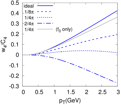
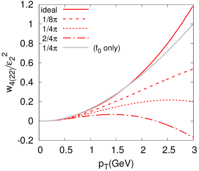
At large $p_{T}$ the non-linear response curves show a characteristic quadratic rise with $p_{T}$, while the linear response curves show a characteristic linear rise. This difference between the non-linear and linear response is known from previous studies of $v_{4}$ Borghini:2005kd . Later, when examining non-linear corrections to $v_{1}$ (see Fig. 6), we will see that the non-linear corrections are most important at high $p_{T}$ and exhibit a characteristic quadratic rise. Comparing Fig. 1(a) and (b), we see that viscous corrections are smaller for the non-linear response $w_{4(22)}(p_{T})/\epsilon_{2}^{2}$, than for the linear response $w_{4}(p_{T})/{\mathcal{C}}_{4}$. This is a generic result as will be discussed in detail in Section III.2.3.

We also note that the linear response curves shown in Fig. 1(a) change sign for sufficiently large viscosity. This is an artifact of the first viscous correction, $\delta f$, and the quadratic ansatz. To see this, we have plotted $w_{4}(p_{T})$ and and $w_{4(22)}(p_{T})$ using only the unmodified distribution function $f_{o}$ in Fig. 1(a) and (b). For large viscosity the $\delta f$ correction to $v_{4}$ and $v_{5}$ is not small compared to the ideal contribution $f_{o}$, and this causes a reduction of the response, which is more pronounced for the higher harmonics, $v_{4}$ and $v_{5}$. In full kinetic theory calculations $w_{4}/{\mathcal{C}}_{4}$ and $w_{5}/{\mathcal{C}}_{5}$ remain positive and approach zero as the viscosity is increased Alver:2010dn . Thus, the negative $w_{4}/{\mathcal{C}}_{4}$ indicates that the first viscous correction has become too large to be trusted. Below, we will simply set the response coefficients to zero when this is the case. Experience with kinetic theory suggests that this ad hoc procedure is not far from what really happens.

III.2.2 Centrality dependence of the response coefficients

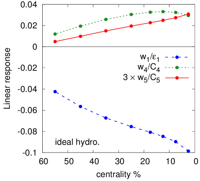
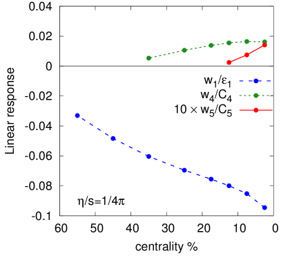
Fig. 2 shows the linear and non-linear response coefficients in ideal and viscous hydrodynamics. There are several salient features contained in these plots. First, note that the magnitude of the linear response coefficient $w_{5}/{\mathcal{C}}_{5}$ is quite small in the viscous case, and $w_{5}/{\mathcal{C}}_{5}$ has been multiplied by ten to make the curves visible. The non-linear response $w_{5(23)}$ coefficient is significantly larger. The implications of this difference will be studied in the next section when we multiply the response coefficients by ${\mathcal{C}}_{5}$ and $\epsilon_{2}\epsilon_{3}$ respectively. Second, all of the response coefficients are reduced by viscosity, especially in non-central collisions.

The viscous $w_{4}/{\mathcal{C}}_{4}$ and $w_{5}/{\mathcal{C}}_{5}$ curves stop abruptly as a function of centrality, since we have truncated the curves when response falls below zero. As discussed above (see Fig. 1), this is because viscous corrections to the thermal distribution function ($\delta f$) become larger for more peripheral collisions, and this correction is magnified by the high harmonic number. We have therefore truncated the $w_{4}$ and $w_{5}$ response curves when the response turns negative. At this point $\delta f$ constitutes an order one correction and can no longer be trusted.

Figure 2: The linear and non-linear response coefficients for ideal and viscous hydro. In the viscous case the curves are truncated when the response coefficients turn negative, i.e. outside of the regime of validity of viscous hydro.

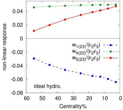
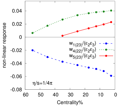
III.2.3 Dependence on viscosity

It is interesting to note that viscous reduction for $w_{1}/\epsilon_{1}$ is smaller than for $w_{4}/{\mathcal{C}}_{4}$ and $w_{5}/{\mathcal{C}}_{5}$. This pattern of viscous corrections for linearized perturbations is studied further in Fig. 3(a). Each linearized perturbation labeled by $n,m$-th cumulant is damped by a factor $\sim\exp(-\Gamma_{n,m}\,\tau_{\rm final})$ relative to ideal hydrodynamics, where $\tau_{\rm final}$ is an estimate for the duration of the event. Analytical work shows that the damping coefficients $\Gamma_{n,m}$ scale as

$$\Gamma_{n,m}\,\tau_{\rm final}\sim\frac{\ell_{\rm mfp}}{L}\left(\frac{n-m}{2}+m\right)^{2}\,,$$ (29)

for a conformal equation of state and a particular background flow Gubser:2010ui . Thus, each power of $r^{2}$ and each harmonic order in eq. (5) increases $(n{-}m)/2{+}m$ by one unit. Our numerical work (Fig. 3(a)) is not limited to the conformal equation of state or the particular background flow of Ref. Gubser:2010ui , and shows that this scaling is reasonably generic Alver:2010dn ; Retinskaya:2012ky . Specifically, the formal estimate given in eq. (29) implies a definite pattern among the viscous corrections to $v_{n}$:

$$-\frac{\Delta w_{1}}{w_{1}^{\rm id}}\simeq-\frac{\Delta w_{2}}{w_{2}^{\rm id}}\propto\,4\,\frac{\eta}{s}\,,\qquad-\frac{\Delta w_{3}}{w_{3}^{\rm id}}\propto\,9\,\frac{\eta}{s}\,,\qquad-\frac{\Delta w_{4}}{w_{4}^{\rm id}}\propto\,16\,\frac{\eta}{s}\,,\qquad-\frac{\Delta w_{5}}{w_{5}^{\rm id}}\propto\,25\,\frac{\eta}{s}\,.$$ (30)

where $\Delta w=w^{\rm viscous}-w^{\rm ideal}$, and $w^{\rm id}$ is the ideal hydro response coefficient. Note, in particular that the viscous corrections $v_{1}$ and $v_{2}$ are similar since $v_{1}$ and $v_{2}$ respond to the dipole asymmetry, $W_{3,1}$, and the ellipticity, $W_{2,2}$, respectively Retinskaya:2012ky . Since the slopes of the $v_{1}:v_{2}:v_{3}:v_{4}:v_{5}$ curves in Fig. 3(a) have approximately the expected ratios $4:4:9:16:25$, our numerical work qualitatively confirms this pattern of viscous corrections.

Figure 3: (a) Linear response coefficients $w_{n}$ as a function of viscosity relative to the ideal response. (b) A comparison of non-linear and linear response coefficients as a function of viscosity. e.g. $w_{5(23)}$ records the $v_{5}$ produces by a combination of $\epsilon_{2}$ and $\epsilon_{3}$. The negative values for large viscosity are spurious, and lie beyond the region of applicability of viscous hydrodynamics.

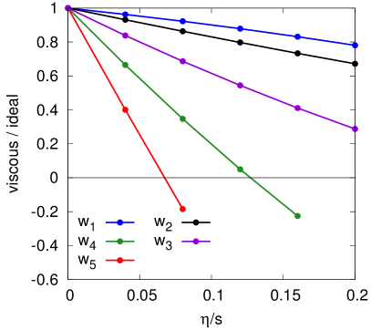
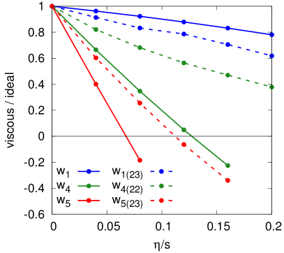
Fig. 3(b) compares the damping rate for the non-linear response coefficients to the corresponding linear response coefficients. Take $w_{5(23)}$ for example. Since $w_{5(23)}$ is of order $~{}v_{2}v_{3}$ we expect the damping of this non-linear perturbation to scale as $\sim e^{-\Gamma_{2,2}\tau}e^{-\Gamma_{3,3}\tau}$, and thus the damping rate $\Gamma_{5(23)}$ is expected to scale as

$$\Gamma_{5(23)}\sim\Gamma_{2,2}+\Gamma_{3,3}\,.$$ (31)

Thus, we expect the non-linear and linear response coefficients for $v_{5}$ to scale as

$$-\frac{\Delta w_{5(23)}}{w_{5(23)}^{\rm id}}\propto 13\frac{\eta}{s}\,,\qquad-\frac{\Delta w_{5}}{w_{5}^{\rm id}}\propto 25\frac{\eta}{s}\,.$$ (32)

Comparing the slopes of the non-linear and linear response curves in Fig. 3(b), we see that the slope of the $\Delta w_{5(23)}/w_{5(23)}^{\rm id}$ curve is approximately half of the corresponding $\Delta w_{5}/w_{5}^{\rm id}$, and is qualitatively consistent with our heuristic estimate of $13/25$. $w_{4(22)}$ and $w_{4}$ show a similar pattern of viscous corrections. Finally our estimates seem only partially applicable to $v_{1}$. For instance, the reasoning of eq. (31) predicts that the non-linear damping rates, $\Gamma_{1(23)}$ and $\Gamma_{5(23)}$, should be equal. However, the slope of $\Delta w_{1(23)}/w_{1(23)}^{\rm id}$ is significantly smaller than the $\Delta w_{5(23)}/w_{5(23)}^{\rm id}$, and contradicts this reasoning. Clearly, the non-linear viscous damping of $v_{1}$ is a special case which will have to be investigated more completely at a later date.

IV Results and Discussion

IV.1 Results

Having clarified the non-linear hydrodynamic response, we study the phenomenological implications of these response coefficients. Fig. 4 shows $v_{1}$, $v_{4}$ and $v_{5}$ including the linear and non-linear response as outlined in Section II, and is the principal result of this work.

Figure 4: $v_{1}$, $v_{4}$ and $v_{5}$ versus centrality in ideal and viscous hydrodynamics. To keep the ideal and viscous curves on the same scale we have multiplied the viscous $v_{5}$ curves by a factor of two. In the viscous case, the linear response is neglected when the response coefficients turn negative, i.e. outside of the region of applicability of viscous hydrodynamics.

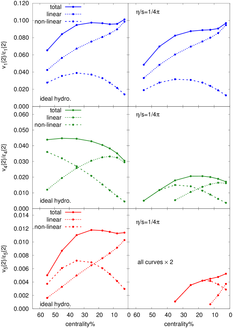
Examining this figures we see that the non-linear response is an important correction for $v_{1}$, and essential for $v_{4}$ and $v_{5}$. The contribution of the non-linear response to the total flow increases towards peripheral collisions, and for $v_{4}$ and $v_{5}$ is of order $50\%$ in mid-peripheral collisions. This is roughly compatible with simulation results from event-by-event hydrodynamics Qiu:2011iv ; Gardim:2011xv . Especially for viscous hydrodynamics and for $v_{5}$, the linear response is negligible in all but the most central bin. Even in the most central bin, the non-linear contribution to $v_{5}$ is about 50% of the total. It is notable, if expected, that for $v_{1}$ viscosity reduces the non-linear contribution relative to the total, while for $v_{4}$ and $v_{5}$ viscosity increases the non-linear contributions. This is consistent with the discussion given in Section II.2.

It will be quite interesting to measure the complete set of event planes $(\Psi_{1},\Psi_{2},\Psi_{3},\Psi_{4},\Psi_{5})$ and their inter-correlations. These measurements will place a strong experimental constraint on the relative of importance of the non-linear response ATLASCorrelations . For example, if the non-linear response is dominant (as implied by the viscous $v_{5}$ curves), then a stronger than geometric correlation is expected for certain experimental averages, e.g. $\left\langle\cos(5\Psi_{5}-3\Psi_{3}-2\Psi_{2})\right\rangle$.

Next we examine the $p_{T}$ dependence of the $v_{1}$,$v_{4}$ and $v_{5}$. Since $v_{4}$ and $v_{5}$ are dominated by the non-linear response we will present our results by scaling $v_{2}^{2}$ and $v_{2}v_{3}$ respectively. Many of the points raised in this and the next paragraph are familiar from earlier studies of $v_{4}$ in the $\Psi_{2}$ plane. In particular, the importance of non-linearities and fluctuations in determining the experimental $v_{4}/v_{2}^{2}$ ratio was understood previously Borghini:2005kd ; Gombeaud:2009ye .

First we note that according to an old argument by Borghini and Ollitrault Borghini:2005kd , $v_{4}/v_{2}^{2}$ should approach $1/2$ at large momentum in ideal hydrodynamics for any given event due to the non-linearities inherent in the phase space distribution. Their result is easily generalized to $v_{5}$, $v_{5}=v_{2}v_{3}$. The argument follows by computing the freezeout distribution in a saddle point approximation Blaizot:1986bh , and can be schematically understood by examining the thermal factor in an approximately radially symmetric flow profile. The transverse flow vector as a function of the spatial azimuthal angle $\phi$ relative to the reaction plane is

$$\vec{u}_{T}=(u^{x},u^{y})\simeq(u_{T}(\phi)\cos\phi,u_{T}(\phi)\sin\phi)\,,$$ (33)

where in the second step we have assumed that the flow is approximately radially symmetric. The transverse flow velocity is then expanded in harmonics

$$u_{T}(\phi)=u_{T}^{(0)}+2u_{T}^{(2)}\cos 2\phi+2u_{T}^{(4)}\cos 4\phi+\mbox{other harmonics}\,,$$ (34)

and the thermal factor with $\vec{p}=(p_{T}\cos\phi_{\bm{p}},p_{T}\sin\phi_{\bm{p}})$ reads

$$e^{\vec{p}\cdot\vec{u}/T}\simeq e^{\frac{p_{T}}{T}u_{T}^{(0)}\cos(\phi_{\bm{p}}-\phi)}\left[1+\frac{2p_{T}}{T}u_{T}^{(2)}\cos 2\phi+\frac{1}{2}\left(\frac{2p_{T}}{T}u_{T}^{(2)}\cos 2\phi\right)^{2}+\ldots\right]\,,$$ (35)

$$\simeq e^{\frac{p_{T}}{T}u_{T}^{(0)}(\cos\phi_{\bm{p}}-\phi)}\left[1+\frac{2p_{T}}{T}u_{T}^{(2)}\cos 2\phi_{\bm{p}}+\left(\frac{p_{T}}{T}u_{T}^{(2)}\right)^{2}\cos 4\phi_{\bm{p}}+\ldots\right]\,.$$ (36)

The leading exponential strongly correlates coordinate space angle $\phi$ and the momentum space angle $\phi_{\bm{p}}$. In the second line we have anticipated the saddle point approximation, (which realizes this correlation) and set $\phi\simeq\phi_{\bm{p}}$ in the post-exponent. The second term in square brackets determines the linear response coefficient $w_{2}$ and rises linearly with momentum, $w_{2}\sim p_{T}u_{T}^{(2)}/T$. The third term determines the non-linear response coefficient $w_{4(22)}$, and grows quadratically with momentum, $w_{4(22)}\sim{\textstyle\frac{1}{2}}(p_{T}u_{T}^{(2)}/T)^{2}$. At high $p_{T}$ this quadratic growth overwhelms the (neglected) linear response due to $u_{T}^{(4)}$, and leads to the characteristic relation $v_{4}=\frac{1}{2}v_{2}^{2}$. An entirely identical argument shows that $v_{5}=v_{2}v_{3}$ at high momentum in ideal hydrodynamics.

The Borghini-Ollitrault argument given above shows that the response coefficients in ideal hydro should asymptote at large momentum,

$$\frac{w_{4(22)}/\epsilon_{2}^{2}}{(w_{2}/\epsilon_{2})^{2}}\xrightarrow[{p_{T}\rightarrow\infty}]{}\frac{1}{2}\,,\qquad\frac{w_{5(23)}/(\epsilon_{2}\epsilon_{3})}{(w_{2}/\epsilon_{2})(w_{3}/\epsilon_{3})}\xrightarrow[{p_{T}\rightarrow\infty}]{}1\,.$$ (37)

When fluctuations are included these asymptotic relations are modified Gombeaud:2009ye :

$$\frac{v_{4}\{2\}}{v_{2}\{2\}^{2}}\xrightarrow[{p_{T}\rightarrow\infty}]{}\frac{1}{2}\left(\frac{\left\langle\epsilon_{2}^{4}\right\rangle}{\left\langle\epsilon_{2}^{2}\right\rangle^{2}}\right)^{1/2}\,,\qquad\frac{v_{5}\{2\}}{v_{2}\{2\}v_{3}\{2\}}\xrightarrow[{p_{T}\rightarrow\infty}]{}\left(\frac{\left\langle(\epsilon_{2}\epsilon_{3})^{2}\right\rangle}{\left\langle\epsilon_{2}^{2}\right\rangle\left\langle\epsilon_{3}^{2}\right\rangle}\right)^{1/2}\,.$$ (38)

Previous studies of $v_{4}$ in the $\Psi_{2}$ plane (see Section II.2) have shown that such geometrical factors are essential to reproducing the centrality dependence of $v_{4}/v_{2}^{2}$ Gombeaud:2009ye . The following table records the geometrical ratios in eq. (38) as a function of centrality.

Centrality %	2.5	7.5	12.5	17.5	25.0	35.0	45.0	55.5
$\sqrt{{\left\langle\epsilon_{2}^{4}\right\rangle}/{\left\langle\epsilon_{2}^{2}\right\rangle^{2}}}$	1.40	1.33	1.26	1.22	1.20	1.18	1.17	1.16
$\sqrt{{\left\langle(\epsilon_{2}\epsilon_{3})^{2}\right\rangle}/({\left\langle\epsilon_{2}^{2}\right\rangle\left\langle\epsilon_{3}^{2}\right\rangle})}$	0.99	0.97	0.96	0.95	0.94	0.93	0.930	0.92
$\sqrt{{\left\langle\epsilon_{2}^{2}\right\rangle}/{\left\langle\epsilon_{1}^{2}\right\rangle}}$	2.12	2.78	3.22	3.46	3.56	3.40	3.04	2.64

We have found that rather large $p_{T}$ is needed to see the non-linear limit given by eq. (38). In the current framework, the linear and non-linear response terms, and their interference, determine the full result

$$v_{4}\{2\}(p_{T})=\frac{\left\langle\!\left\langle w_{4}(p_{T})w_{4}+w_{4(22)}(p_{T})w_{4(22)}+[w_{4}(p_{T})w_{4(22)}+w_{4(22)}(p_{T})w_{4}]\cos 4(\Phi_{4}-\Phi_{2})\right\rangle\!\right\rangle}{v_{4}\{2\}}$$ (39)

Fig. 5 shows the complete result for $v_{4}\{2\}/v_{2}\{2\}^{2}$

Figure 5: Results for $v_{4}$ and $v_{5}$ for ideal and viscous hydrodynamics at various impact parameters. The Borghini-Ollitrault expectation is indicated by the arrows for the ideal $v_{4}$ and $v_{5}$ curves Borghini:2005kd .

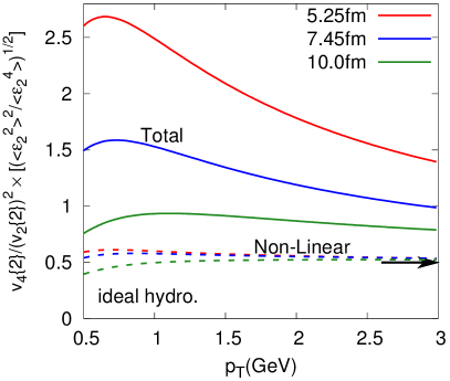
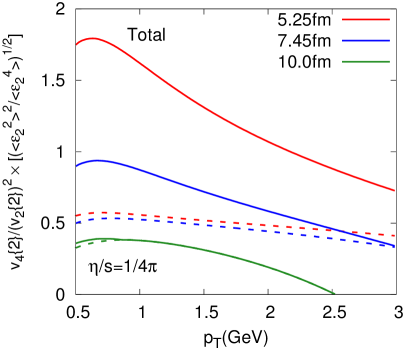
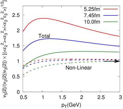
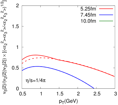
(scaled by $\sqrt{\left\langle\epsilon_{2}^{4}\right\rangle/\left\langle\epsilon_{2}^{2}\right\rangle^{2}}$) for ideal and viscous hydrodynamics. Focusing on the ideal results, we see that full results (the solid lines) approach the non-linear expectation of Borghini and Ollitrault (the dashed line) only very slowly. This is in large part because $w_{4}(p_{T})$ is only qualitatively linear at sub-asymptotic $p_{T}$ and increases almost quadratically at intermediate $p_{T}\sim 1.5\,{\rm GeV}$, momentarily keeping up with the non-linear response. When viscous corrections are included, the non-linear results become dominant in peripheral collisions. Similar results for $v_{5}$ in ideal and viscous hydrodynamics are also shown in Fig. 5. In the viscous case, the non-linear result gives almost the full $v_{5}\{2\}$ for all centrality classes shown.

It is worth noting that the magnitude of the viscous corrections as a function of $p_{T}$ for $v_{4}$ and $v_{5}$ are sensitive to ansatz used for the viscous distribution function, $\delta f$ Luzum:2010ad . In particular, the quadratic ansatz used in this work assumes that the quasi-particle energy loss is independent of momentum, $dp/dt\propto\mbox{const}$. A linear ansatz for $\delta f$ is better motivated for QCD like theories and results in smaller viscous corrections for $v_{4}$ and $v_{5}$ as a function of $p_{T}$ Dusling:2009df . A complete discussion of this point is reserved for future work.

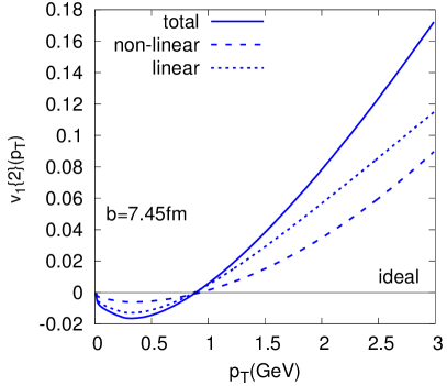
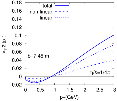
Fig. 6 presents the corresponding analysis for $v_{1}(p_{T})$. We see that the non-linear terms provide a correction to the linear response which grows with $p_{T}$ due to the quadratic dependence of the non-linear response coefficients, $w_{1(23)}\propto p_{T}^{2}$. We note that the viscous corrections are approximately the same for $v_{1}(p_{T})$ and $v_{2}(p_{T})$, as expected from the discussion of viscous corrections given in Section II.2.

Figure 6: $v_{1}(p_{T})\{2\}$ (eq. (22)) in ideal and viscous hydrodynamics from the linear response to ${\epsilon}_{1}$, the non-linear response to ${\epsilon}_{2}{\epsilon}_{3}$, and the total response, eq. (24).

IV.2 Discussion

We have presented a framework of non-linear response to understand the higher harmonics generated in heavy ion collisions. Then we extracted the non-linear response coefficients using ideal and viscous hydrodynamics and studied the dependence on the shear viscosity, in Fig. 2. The pattern of viscous corrections is further analyzed in Fig. 3 and explained in Section III.2. Generally, when the harmonic order is large, the non-linear response is less damped than the corresponding linear response. Thus, when viscosity is included in hydrodynamic simulations, the non-linear response becomes increasingly important for the higher harmonics. This qualitative reasoning is confirmed in Fig. 4 which shows $v_{1}$, $v_{4}$ and $v_{5}$ using linear and non-linear response and is the principal result of this work. We see that the non-linear response is essential for $v_{4}$ and $v_{5}$, and constitutes an important correction for $v_{1}$.

Experimentally, the relative contributions of the linear and non-linear response can be disentangled by measuring $v_{5}$ in the $2\Psi_{2}+3\Psi_{3}$ and $\Psi_{5}$ planes, $i.e.$ by measuring

$$v_{5(23)}\equiv\left\langle\cos(5\phi_{\bm{p}}-2\Psi_{2}-3\Psi_{3})\right\rangle\,,\quad\mbox{and}\quad v_{5(5)}\equiv\left\langle\cos 5(\phi_{\bm{p}}-\Psi_{5})\right\rangle\,.$$ (40)

Although a full discussion of this and similar measurements is reserved for future work, a qualitative expectation based on Fig. 4(e) and (f) is that the $\left\langle\cos(5\Psi_{5}-3\Psi_{3}-2\Psi_{2})\right\rangle$ correlation should be strong compared to the geometric average, and should change rapidly from central to mid-central collisions. Qualitatively, this is precisely what was observed recently by the ATLAS collaboration ATLASCorrelations .

The non-linear response can also be studied by analyzing the $p_{T}$ dependence of the flow harmonics. Fig. 5 and Fig. 6 exhibit $v_{4}(p_{T})$, $v_{5}(p_{T})$, and $v_{1}(p_{T})$. In ideal hydrodynamics at large $p_{T}$ we expect to find $v_{4}={\textstyle\frac{1}{2}}v_{2}^{2}$ on an event by event basis. Our non-linear response coefficients corroborate this non-linear expectation for $v_{4}$ and an analogous relation for $v_{5}$, $v_{5}=v_{2}v_{3}$. However, since what is normally measured is $v_{4}\{2\}/(v_{2}\{2\})^{2}$ and not $\left\langle\!\left\langle v_{4}/v_{2}^{2}\right\rangle\!\right\rangle$, this ideal non-linear expectation must be multiplied by $(\left\langle\epsilon_{2}^{4}\right\rangle/\left\langle\epsilon_{2}^{2}\right\rangle^{2})^{1/2}$ when comparing to the experimental data Gombeaud:2009ye . In addition, this expectation of ideal hydrodynamics is broken by viscous corrections, and by the linear response to the fourth order cumulant ${\mathcal{C}}_{4}$ (i.e. $\epsilon_{4}$). When all of these corrections are taken into account, we find that relations such as $v_{4}={\textstyle\frac{1}{2}}v_{2}^{2}$ and $v_{5}=v_{2}v_{3}$ provide only a rough guide to the full result.

Throughout we have assumed perfect correlation between $\Psi_{2}$ and $\Phi_{2}$ and $\Psi_{3}$ and $\Phi_{3}$. This strict correlation is only approximately true. For instance the combination of a $v_{1}$ and a $v_{3}$ can yield a $v_{2}$,

$$v_{2}e^{-i2\Psi_{2}}=w_{2}e^{-i2\Phi_{2}}+w_{2(13)}e^{-i3\Phi_{3}+i\Phi_{1}}\,.$$ (41)

This naturally provides a correlation between the $\Psi_{2}$ and $\Psi_{3}$ plane, although the geometric correlation between $\Phi_{2}$ and $\Phi_{3}$ is negligibly small. Indeed the $(\Psi_{2},\Psi_{3})$ correlation, which was very recently observed by the ATLAS collaboration ATLASCorrelations , is too large to be easily explained with the geometric correlations of the Glauber model. Similarly, assuming that the linear response to $\epsilon_{6}$ is negligible, one could expect that in central collisions $v_{6}$ is determined by the quadratic response to $v_{3}$, while in peripheral collisions $v_{6}$ is determined by a cubic response to $v_{2}$

$$v_{6}e^{-i6\Psi_{6}}=w_{6(222)}e^{-i6\Phi_{2}}+w_{6(33)}e^{-i6\Phi_{3}}\,.$$ (42)

Qualitatively, this pattern is consistent with the observed $(\Psi_{6},\Psi_{3})$ and $(\Psi_{6},\Psi_{2})$ correlations presented in ATLASCorrelations . It will be interesting to see if all of the observed correlations can be quantitatively understood with the non-linear response theory outlined in this paper. A full quantitative comparison with the experimental data is reserved for future work.

Acknowledgments:

We thank J. Y. Ollitrault, and Z. Qiu, and U. Heinz for many constructive and insightful comments. D. Teaney is a RIKEN-RBRC fellow. This work is supported in part by the Sloan Foundation and by the Department of Energy through the Outstanding Junior Investigator program, DE-FG-02-08ER4154.

References

- (1) Sergei A. Voloshin, Arthur M. Poskanzer, and Raimond Snellings, “Collective phenomena in non-central nuclear collisions,” (2008), arXiv:0809.2949 [nucl-ex]
- (2) Derek A. Teaney, “Viscous Hydrodynamics and the Quark Gluon Plasma,” (2009), invited review for ’Quark Gluon Plasma 4’. Editors: R.C. Hwa and X.N. Wang, World Scientific, Singapore., arXiv:0905.2433 [nucl-th]
- (3) Peter F. Kolb and Ulrich W. Heinz, “Hydrodynamic description of ultrarelativistic heavy ion collisions,” (2003), invited review for ’Quark Gluon Plasma 3’. Editors: R.C. Hwa and X.N. Wang, World Scientific, Singapore., arXiv:nucl-th/0305084 [nucl-th]
- (4) J. Takahashi et al., “Topology studies of hydrodynamics using two particle correlation analysis,” Phys. Rev. Lett. 103, 242301 (2009), arXiv:0902.4870 [nucl-th]
- (5) Paul Sorensen, “Implications of space-momentum correlations and geometric fluctuations in heavy-ion collisions,” J.Phys.G G37, 094011 (2010), arXiv:1002.4878 [nucl-ex]
- (6) G.L. Ma, S. Zhang, Y.G. Ma, H.Z. Huang, X.Z. Cai, et al., “Di-hadron azimuthal correlation and mach-like cone structure in parton/hadron transport model,” Phys.Lett. B641, 362–367 (2006), arXiv:nucl-th/0601012 [nucl-th]
- (7) B. Alver and G. Roland, “Collision geometry fluctuations and triangular flow in heavy-ion collisions,” Phys.Rev. C81, 054905 (2010), arXiv:1003.0194 [nucl-th]
- (8) Matthew Luzum, “Collective flow and long-range correlations in relativistic heavy ion collisions,” Phys.Lett. B696, 499–504 (2011), arXiv:1011.5773 [nucl-th]
- (9) Derek Teaney and Li Yan, “Triangularity and Dipole Asymmetry in Heavy Ion Collisions,” Phys.Rev. C83, 064904 (2011), arXiv:1010.1876 [nucl-th]
- (10) Rajeev S. Bhalerao, Matthew Luzum, and Jean-Yves Ollitrault, “Determining initial-state fluctuations from flow measurements in heavy-ion collisions,” Phys.Rev. C84, 034910 (2011), arXiv:1104.4740 [nucl-th]
- (11) The ATLAS Collaboration, “Measurement of reaction plane correlations in Pb-Pb collisions at =2.76 TeV,” (May May, 2012), ATLAS-CONF-2012-049. See also https://cdsweb.cern.ch/record/1451882
- (12) Burak Han Alver, Clement Gombeaud, Matthew Luzum, and Jean-Yves Ollitrault, “Triangular flow in hydrodynamics and transport theory,” Phys. Rev. C82, 034913 (2010), arXiv:1007.5469 [nucl-th]
- (13) Zhi Qiu and Ulrich W. Heinz, “Event-by-event shape and flow fluctuations of relativistic heavy-ion collision fireballs,” Phys.Rev. C84, 024911 (2011), arXiv:1104.0650 [nucl-th]
- (14) Fernando G. Gardim, Frederique Grassi, Matthew Luzum, and Jean-Yves Ollitrault, “Mapping the hydrodynamic response to the initial geometry in heavy-ion collisions,” Phys.Rev. C85, 024908 (2012), arXiv:1111.6538 [nucl-th]
- (15) Bjorn Schenke, Sangyong Jeon, and Charles Gale, “Elliptic and triangular flow in event-by-event (3+1)D viscous hydrodynamics,” Phys. Rev. Lett. 106, 042301 (2011), arXiv:1009.3244 [hep-ph]
- (16) Hannah Petersen, Guang-You Qin, Steffen A. Bass, and Berndt Muller, “Triangular flow in event-by-event ideal hydrodynamics in Au+Au collisions at GeV,” Phys. Rev. C82, 041901 (2010), arXiv:1008.0625 [nucl-th]
- (17) Fernando G. Gardim, Frederique Grassi, Yogiro Hama, Matthew Luzum, and Jean-Yves Ollitrault, “Directed flow at mid-rapidity in event-by-event hydrodynamics,” Phys. Rev. C83, 064901 (2011), arXiv:1103.4605 [nucl-th]
- (18) Hannu Holopainen, Harri Niemi, and Kari J. Eskola, “Event-by-event hydrodynamics and elliptic flow from fluctuating initial state,” Phys. Rev. C83, 034901 (2011), arXiv:1007.0368 [hep-ph]
- (19) K. Werner, Iu. Karpenko, T. Pierog, M. Bleicher, and K. Mikhailov, “Event-by-Event Simulation of the Three-Dimensional Hydrodynamic Evolution from Flux Tube Initial Conditions in Ultrarelativistic Heavy Ion Collisions,” Phys. Rev. C82, 044904 (2010), arXiv:1004.0805 [nucl-th]
- (20) Jean-Yves Ollitrault, “Anisotropy as a signature of transverse collective flow,” Phys. Rev. D46, 229–245 (1992)
- (21) Steven S. Gubser and Amos Yarom, “Conformal hydrodynamics in Minkowski and de Sitter spacetimes,” Nucl.Phys. B846, 469–511 (2011), arXiv:1012.1314 [hep-th]
- (22) Peter F. Kolb, “v(4): A Small, but sensitive observable for heavy ion collisions,” Phys.Rev. C68, 031902 (2003), arXiv:nucl-th/0306081 [nucl-th]
- (23) Nicolas Borghini and Jean-Yves Ollitrault, “Momentum spectra, anisotropic flow, and ideal fluids,” Phys.Lett. B642, 227–231 (2006), arXiv:nucl-th/0506045 [nucl-th]
- (24) Clement Gombeaud and Jean-Yves Ollitrault, “Effects of flow fluctuations and partial thermalization on ,” Phys. Rev. C81, 014901 (2010), arXiv:0907.4664 [nucl-th]
- (25) Matthew Luzum, Clement Gombeaud, and Jean-Yves Ollitrault, “ in ideal and viscous hydrodynamics simulations of nuclear collisions at the BNL Relativistic Heavy Ion Collider (RHIC) and the CERN Large Hadron Collider (LHC),” Phys.Rev. C81, 054910 (2010), arXiv:1004.2024 [nucl-th]
- (26) Matthew Luzum and Jean-Yves Ollitrault, “Constraining the viscous freeze-out distribution function with data obtained at the BNL Relativistic Heavy Ion Collider (RHIC),” Phys.Rev. C82, 014906 (2010), arXiv:1004.2023 [nucl-th]
- (27) Yuting Bai (STAR Collaboration), “The Anisotropic flow coefficients v(2) and v(4) in Au + Au collisions at RHIC,” J.Phys.G G34, S903–906 (2007), arXiv:nucl-ex/0701044 [nucl-ex]
- (28) A. Adare et al. (PHENIX), “Elliptic and hexadecapole flow of charged hadrons in Au+Au collisions at ,” Phys. Rev. Lett. 105, 062301 (2010), arXiv:1003.5586 [nucl-ex]
- (29) B. Alver, M. Baker, C. Loizides, and P. Steinberg, “The PHOBOS Glauber Monte Carlo,” (2008), arXiv:0805.4411 [nucl-ex]
- (30) Rajeev S. Bhalerao, Matthew Luzum, and Jean-Yves Ollitrault, “Understanding anisotropy generated by fluctuations in heavy-ion collisions,” Phys.Rev. C84, 054901 (2011), arXiv:1107.5485 [nucl-th]
- (31) Jiangyong Jia and Derek Teaney, “Study on initial geometry fluctuations via participant plane correlations in heavy ion collisions: part II,” (2012), arXiv:1205.3585 [nucl-ex]
- (32) Rudolf Baier, Paul Romatschke, Dam Thanh Son, Andrei O. Starinets, and Mikhail A. Stephanov, “Relativistic viscous hydrodynamics, conformal invariance, and holography,” JHEP 0804, 100 (2008), arXiv:0712.2451 [hep-th]
- (33) K. Dusling and D. Teaney, “Simulating elliptic flow with viscous hydrodynamics,” Phys.Rev. C77, 034905 (2008), arXiv:0710.5932 [nucl-th]
- (34) Sayantani Bhattacharyya, Veronika E Hubeny, Shiraz Minwalla, and Mukund Rangamani, “Nonlinear Fluid Dynamics from Gravity,” JHEP 0802, 045 (2008), arXiv:0712.2456 [hep-th]
- (35) Matthew Luzum and Paul Romatschke, “Conformal Relativistic Viscous Hydrodynamics: Applications to RHIC results at ,” Phys. Rev. C78, 034915 (2008), arXiv:0804.4015 [nucl-th]
- (36) Derek Teaney, “The Effects of viscosity on spectra, elliptic flow, and HBT radii,” Phys.Rev. C68, 034913 (2003), arXiv:nucl-th/0301099 [nucl-th]
- (37) Kevin Dusling, Guy D. Moore, and Derek Teaney, “Radiative energy loss and v(2) spectra for viscous hydrodynamics,” Phys.Rev. C81, 034907 (2010), arXiv:0909.0754 [nucl-th]
- (38) Ekaterina Retinskaya, Matthew Luzum, and Jean-Yves Ollitrault, “Directed flow at midrapidity in Pb+Pb collisions,” Phys.Rev.Lett. 108, 252302 (2012), arXiv:1203.0931 [nucl-th]
- (39) J.P. Blaizot and Jean-Yves Ollitrault, “Hydrodynamics of a quark qluon plasma undergoing a phase transition,” Nucl.Phys. A458, 745 (1986)