The Hausdorff dimension of the CLE gasket

Abstract

The conformal loop ensemble $\mathrm{CLE}_{\kappa}$ is the canonical conformally invariant probability measure on noncrossing loops in a proper simply connected domain in the complex plane. The parameter $\kappa$ varies between $8/3$ and $8$; $\mathrm{CLE}_{8/3}$ is empty while $\mathrm{CLE}_{8}$ is a single space-filling loop. In this work, we study the geometry of the $\mathrm{CLE}$ gasket, the set of points not surrounded by any loop of the $\mathrm{CLE}$. We show that the almost sure Hausdorff dimension of the gasket is bounded from below by $2-(8-\kappa)(3\kappa-8)/(32\kappa)$ when $4<\kappa<8$. Together with the work of Schramm–Sheffield–Wilson [Comm. Math. Phys. 288 (2009) 43–53] giving the upper bound for all $\kappa$ and the work of Nacu–Werner [J. Lond. Math. Soc. (2) 83 (2011) 789–809] giving the matching lower bound for $\kappa\leq 4$, this completes the determination of the $\mathrm{CLE}_{\kappa}$ gasket dimension for all values of $\kappa$ for which it is defined. The dimension agrees with the prediction of Duplantier–Saleur [Phys. Rev. Lett. 63 (1989) 2536–2537] for the FK gasket.

, and t1Supported in part by a Dept. of Defense (AFOSR) NDSEG Fellowship.

1 Introduction

The conformal loop ensemble $\mathrm{CLE}_{\kappa}$ is the canonical conformally invariant measure on countably infinite collections of noncrossing loops in a proper simply connected domain $D$ in $\mathbb{C}$ MR2494457 , SWCLE . It is the loop analogue of $\mathrm{SLE}_{\kappa}$, the canonical conformally invariant measure on noncrossing paths. Whereas $\mathrm{SLE}_{\kappa}$ arises as the scaling limit of a single macroscopic interface of many two-dimensional discrete models MR1776084 , MR2044671 , MR2227824 , MR2322705 , MR2486487 , arXiv10101356 , MR2680496 , chelkak-smirnov , CDCHKS , $\mathrm{CLE}_{\kappa}$ describes the limit of all of the interfaces simultaneously. The parameter $\kappa$ varies between $8/3$ and $8$; $\mathrm{CLE}_{8/3}$ is empty while $\mathrm{CLE}_{8}$ is a single space-filling loop. $\mathrm{CLE}_{\kappa}$ for $\kappa\in(8/3,4]$ consists of disjoint simple loops, while for $\kappa\in(4,8]$ the loops intersect both themselves and each other (but are noncrossing). $\mathrm{CLE}_{3}$ and $\mathrm{CLE}_{16/3}$ are the scaling limits of the cluster boundaries in the square lattice critical Ising spin BDCHISINGCLE and FK-Ising KempSmirFKISINGCLE models, respectively, and $\mathrm{CLE}_{6}$ is the scaling limit of the cluster boundaries in critical percolation on the triangular lattice MR2227824 , MR2249794 . $\mathrm{CLE}_{4}$ is the scaling limit of the level sets of the two-dimensional discrete Gaussian free field MSDGFFCLE .

There are two different constructions of $\mathrm{CLE}_{\kappa}$. In the first construction, due to Werner MR2023758 and applicable for $\kappa\in[8/3,4]$, the loop ensemble is given by the outer boundaries of Brownian loop soup clusters. In this paper, we make use of the second construction, proposed by Sheffield MR2494457 and applicable for $\kappa\in[8/3,8]$, based on branching $\mathrm{SLE}_{\kappa}(\kappa-6)$. These constructions have been proved equivalent for $\kappa\in[8/3,4]$ SWCLE (see also werner-wucle-exploration ).

Figure 1: Under the $O(n)$ model, a loop configuration $\omega$ has probability proportional to $x^{e(\omega)}n^{\ell(\omega)}$ where $\ell(\omega)$ is the number of loops in $\omega$ and $e(\omega)$ is the total length of all the loops. For $0\leq n\leq 2$, there is a critical value $x_{c}\equiv x_{c}(n)$ at which the $O(n)$ model has a “dilute phase,” believed to converge to $\mathrm{CLE}_{\kappa}$ with $n=-2\cos(4\pi/\kappa)$, $8/3\leq\kappa\leq 4$. The $O(n)$ model at $x>x_{c}$ is in a “dense phase,” again believed to converge to $\mathrm{CLE}_{\kappa}$ with $n=-2\cos(4\pi/\kappa)$, but now with $4\leq\kappa\leq 8$. Critical site percolation on the triangular lattice (left panel) corresponds to the (dense phase) $O(n)$ model on the honeycomb lattice with $n=x=1$ (center panel). Its gasket (right panel) is a discretization of the $\mathrm{CLE}_{6}$ gasket.

Figure 2: Discrete simulations of the $\mathrm{CLE}_{\kappa}$ carpet ($\kappa\in[8/3,4]$) or gasket ($\kappa\in(4,8]$) $\mathcal{G}_{\kappa}$ for $\kappa\in\{3,4,16/3,6\}$. The discretized $\mathcal{G}_{\kappa}$ (indicated in black above) is given by the set of points not surrounded by any cluster boundary loop of a discrete configuration sampled from a model known to converge to $\mathrm{CLE}_{\kappa}$. Note $\mathcal{G}_{4}\subseteq\mathcal{G}_{3}$ in our figures because the OR-Ising configuration used in (a) is the binary OR of two independent Ising configurations, one of which is used in (b).

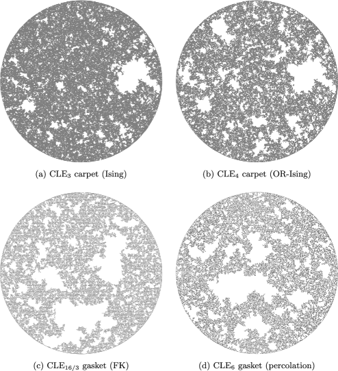
Let $\Gamma$ be a $\mathrm{CLE}_{\kappa}$ in $D$. The carpet ($\kappa\in[8/3,4]$) or gasket ($\kappa\in(4,8]$) $\mathcal{G}$ of $\Gamma$ is the set of points not surrounded by any loop of $\Gamma$. (In analogy with the Sierpiński carpet and gasket, we call $\mathcal{G}$ a carpet or gasket according to whether the loops of $\Gamma$ are disjoint or intersecting, although occasionally we loosely use gasket for both.) Since a.s. every neighborhood intersects a loop, $\mathcal{G}$ is given equivalently by the closure of the union of the outermost loops of $\Gamma$. Figure 1 shows the gasket for a discrete model, critical site percolation, that converges to $\mathrm{CLE}_{6}$. Figure 2 shows discrete simulations of $\mathcal{G}$ for $\kappa=3$ (Ising model), $\kappa=4$ (OR of two independent Ising models, see SWCLE , Proposition 10.2), $\kappa=16/3$ (FK-Ising model), and $\kappa=6$ (critical percolation). The main result of this article is the following theorem.

Theorem 1.1

Fix $\kappa\in(4,8)$ and let $\Gamma$ be a $\mathrm{CLE}_{\kappa}$ in a proper simply connected domain $D$ in $\mathbb{C}$. Then with probability one the Hausdorff dimension of the gasket $\mathcal{G}$ of $\Gamma$ is

$$2-\frac{(8-\kappa)(3\kappa-8)}{32\kappa}.$$ (1)

The formula (1) was first derived in the context of the $O(n)$ model by Duplantier and Saleur PhysRevLett632536 , PhysRevLett64493 , who predicted the fractal dimension of the $O(n)$ gasket (for $n\leq 2$) using nonrigorous Coulomb gas methods. The scaling limit of the $O(n)$ model is believed to be $\mathrm{CLE}_{\kappa}$, where $n=-2\cos(4\pi/\kappa)$ (MR2153402 , Conjecture 9.7, MR2494457 , Section 2.3). There are two values of $\kappa$ associated to each $n<2$, corresponding to the “dilute” ($\kappa<4$) and “dense” ($\kappa>4$) phases of the $O(n)$ model. For further background see KN04 .

Schramm, Sheffield, and Wilson MR2491617 showed that for all $8/3<\kappa<8$,(1) gives the expectation dimension of $\mathcal{G}$, the growth exponent of the expected number of balls of radius $\varepsilon$ needed to cover $\mathcal{G}$: this (a.s.) upper bounds the Minkowski dimension which in turn upper bounds the Hausdorff dimension. (The expectation dimension for $\kappa=6$ was derived earlier by Lawler, Schramm and Werner LSWone-arm .) Nacu and Werner MR2802511 used the Brownian loop soup construction to derive the matching lower bound for the $\mathrm{CLE}_{\kappa}$ carpets ($\kappa\leq 4$).

A lower bound on the Hausdorff dimension of a random fractal set is obtained (by standard arguments) from a second moment estimate controlling the probability that two given points lie near the set. The complicated geometry of $\mathrm{CLE}$ loops prevents us from applying the second moment method directly to $\mathcal{G}$, and instead we use a “multi-scale refinement” MR2123929 : we establish that with arbitrarily small loss in the Hausdorff dimension we can restrict to special classes of points in $\mathcal{G}$ whose correlation structure at all scales can be controlled.

Outline

In Section 2, we review Sheffield’s branching $\mathrm{SLE}_{\kappa}(\kappa-6)$ construction of $\mathrm{CLE}_{\kappa}$ [taking $\kappa\in(4,8)$], with an emphasis on its dependency structure. In Section 3, we prove Theorem 1.1.

2 Preliminaries

In this section, we review the exploration tree construction of $\mathrm{CLE}_{\kappa}$ for $\kappa\in(4,8)$ given in MR2494457 and then collect several useful estimates for conformal maps.

2.1 The continuum exploration tree

We begin by briefly recalling the definition of the $\mathrm{SLE}_{\kappa}$ and $\mathrm{SLE}_{\kappa}(\rho)$ processes. There are many excellent surveys on the subject (e.g., W03 , MR2129588 ) to which we refer the reader for a more detailed introduction. The radial Loewner evolution in the unit disk $\mathbb{D}$ is given by the differential equation

$$\dot{g}_{t}(z)=-g_{t}(z)\frac{g_{t}(z)+W_{t}}{g_{t}(z)-W_{t}},\qquad g_{0}(z)=z,$$ (2)

where $W_{t}$ is a continuous function which takes values in $\partial\mathbb{D}$. We refer to $W_{t}$ as the driving function of the Loewner evolution. For $z\in\mathbb{D}$, let

$$T^{z}\equiv\sup\bigl{\{}t\geq 0\dvtx\bigl{|}g_{t}(z)\bigr{|}<1\bigr{\}}$$

and

$$K_{t}\equiv\bigl{\{}z\in\mathbb{D}\dvtx T^{z}\leq t\bigr{\}}.$$

For each $t\geq 0$, $g_{t}$ is the unique conformal transformation $\mathbb{D}\setminus K_{t}\to\mathbb{D}$ with $g_{t}(0)=0$ and $g_{t}^{\prime}(0)>0$. The (random) growth process $(K_{t})_{t\geq 0}$ associated with $W_{t}=\exp(i\sqrt{\kappa}B_{t})$, where $B_{t}$ is a standard Brownian motion, is the radial $\mathrm{SLE}_{\kappa}$ process introduced by Schramm MR1776084 . Time is parametrized by negative log-conformal radius, that is, $g_{t}^{\prime}(0)=e^{t}$. It was proved by Rohde and Schramm MR2153402 ($\kappa\neq 8$) and Lawler, Schramm, and Werner MR2044671 ($\kappa=8$) that there is a curve $\eta\dvtx[0,\infty)\to\overline{\mathbb{D}}$ starting at $\eta(0)=1$ such that $\mathbb{D}\setminus K_{t}$ is the unique connected component of $\mathbb{D}\setminus\eta[0,t]$ containing $0$: we say that $\eta$ generates the process $K_{t}$ and call $\eta$ the radial $\mathrm{SLE}_{\kappa}$ trace. In this setting, $W_{t}=\lim_{z\to\eta(t)}g_{t}(z)$, where the limit is taken with $z\in\mathbb{D}\setminus K_{t}$. For $\kappa<8$, Lawler lawlerendpoint proved that $\lim_{t\to\infty}\eta(t)=0$, so $\eta\dvtx[0,\infty]\to\overline{\mathbb{D}}$ defines a curve traveling from $\eta(0)=1$ to $\eta(\infty)=0$ in $\overline{\mathbb{D}}$.

Let $D$ be a proper simply connected domain in $\mathbb{C}$. For any conformal transformation $f\dvtx\mathbb{D}\to D$, we take the image of radial $\mathrm{SLE}_{\kappa}$ in $\mathbb{D}$ under $f$ to be the definition of radial $\mathrm{SLE}_{\kappa}$ in $D$ from $f(1)$ to $f(0)$, with $f(1)$ interpreted as a prime end. If $f$ extends continuously to $\overline{\mathbb{D}}$ (equivalently if $\partial D$ is given by a closed curve, see MR1217706 , Theorem 2.1), then radial $\mathrm{SLE}_{\kappa}$ in $D$ is a.s. a continuous curve. It was proved by Garban, Rohde and Schramm MR2891697 that radial $\mathrm{SLE}_{\kappa}$ with $\kappa<8$ in a general proper simply connected domain is a.s. continuous except possibly at its starting point.

We now describe the radial $\mathrm{SLE}_{\kappa}(\rho)$ processes, a natural generalization of radial $\mathrm{SLE}_{\kappa}$ first introduced in MR1992830 , Section 8.3. For $w,o\in\partial\mathbb{D}$, radial $\mathrm{SLE}_{\kappa}(\rho)$ with starting configuration $(w,o)$ is the (random) growth process associated with the solution of (2) where the driving function solves the SDE

$$dW_{t}=-\frac{\kappa}{2}W_{t}\,dt+i\sqrt{\kappa}W_{t}\,dB_{t}-\frac{\rho}{2}W_{t}\frac{W_{t}+O_{t}}{W_{t}-O_{t}}\,dt,\qquad W_{0}=w$$ (3)

with $O_{t}=g_{t}(o)$, the force point. It is easy to see that (3) has a unique solution up to time $\tau_{=}\equiv\inf\{t\geq 0\dvtx W_{t}=O_{t}\}$.

The weight $\rho=\kappa-6$ is special because it arises as a coordinate change of ordinary chordal $\mathrm{SLE}_{\kappa}$ from $w$ targeted at $o$. A consequence is that radial $\mathrm{SLE}_{\kappa}(\kappa-6)$ is target invariant: radial $\mathrm{SLE}_{\kappa}(\kappa-6)$ in $\mathbb{D}$ with starting configuration $(w,o)$ and target $a\in\mathbb{D}$ has the same law (modulo time change) as an ordinary chordal $\mathrm{SLE}_{\kappa}$ in $\mathbb{D}$ from $w$ to $o$, up to the first time the curve disconnects $a$ and $o$ MR2188260 .

We now explain how to construct a solution to (3) which is defined even after time $\tau_{=}$. A more detailed treatment is provided in MR2494457 , Section 3; we give here a brief summary following MR2491617 . For $\rho>-\kappa/2-2$, there is a random continuous process $\theta_{t}$ taking values in $[0,2\pi]$ which evolves according to the SDE

$$d\theta_{t}=\sqrt{\kappa}\,dB_{t}+\frac{\rho+2}{2}\cot(\theta_{t}/2)\,dt$$ (4)

on each interval of time for which $\theta_{t}\notin\{0,2\pi\}$, and is instantaneously reflecting at the endpoints, that is, the set $\{t\dvtx\theta_{t}\in\{0,2\pi\}\}$ has Lebesgue measure zero. (This diffusion was studied in LSWone-arm for $\rho=0$.) In other words, $\theta_{t}$ is a random continuous process adapted to the filtration of $B_{t}$ which a.s. satisfies

$$\partial_{t}[\theta_{t}-\sqrt{\kappa}B_{t}]=\frac{\rho+2}{2}\cot(\theta_{t}/2)$$

for all $t$ for which the right-hand side is finite. The law of this process is uniquely determined by $\theta_{0}$, and moreover the process is pathwise unique MR2494457 , Proposition 4.2. It then follows from the strong Markov property of Brownian motion that $\theta_{t}$ has the strong Markov property.

When $\rho\geq\kappa/2-2$, the $\theta_{t}$ process governed by SDE (4) is repelled so strongly by $0$ and $2\pi$ that it almost surely never reaches either endpoint. When $\rho=-2$ the diffusion $\theta_{t}$ is simply reflected Brownian motion. When $\rho<-2$, the $\theta_{t}$ process is attracted to the singularity and its analysis requires more care, but it still makes sense when $\rho>-\kappa/2-2$ MR2494457 , MR2491617 . When $\rho\leq-\kappa/2-2$, the $\theta_{t}$ process is attracted so strongly to the endpoints that once it hits either one it remains glued there. In the intermediate regime, $-\kappa/2-2<\rho<\kappa/2-2$, the $\theta_{t}$ process hits the endpoints $0$ and $2\pi$, but is instantaneously reflecting. When $\rho=\kappa-6$, this corresponds to the range $8/3<\kappa<8$.

We then set

$$\arg W_{t}=\arg w+\sqrt{\kappa}B_{t}+\frac{\rho}{2}\int_{0}^{t}\cot(\theta_{s}/2)\,ds.$$ (5)

That the above integral is a.s. finite follows by the comparison of $\theta_{t}/\sqrt{\kappa}$ [resp., $(2\pi-\theta_{t})/\sqrt{\kappa}$] with a $\delta$-dimensional Bessel process, as described above; see, for example, the proof of Lemma 3.4. We then define radial $\mathrm{SLE}_{\kappa}(\rho)$ in $\mathbb{D}$ with starting configuration $(w,o)$ to be the solution to (2) with driving function $W_{t}$ defined by (5). The force point $O_{t}\equiv g_{t}(o)$ satisfies $W_{t}=O_{t}e^{i\theta_{t}}$, and we interpret $\theta_{t}=0$ as $O_{t}=W_{t}e^{i0^{-}}$ ($\arg O_{t}$ just below $\arg W_{t}$) and similarly $\theta_{t}=2\pi$ as $O_{t}=W_{t}e^{i0^{+}}$. For $\rho\geq\kappa/2-2$, the laws of radial $\mathrm{SLE}_{\kappa}(\rho)$ and ordinary radial $\mathrm{SLE}_{\kappa}$ are mutually absolutely continuous up to any fixed positive time, so $\mathrm{SLE}_{\kappa}(\rho)$ is a.s. generated by a curve by the result of MR2153402 . In MSIMAG , it is established that $\mathrm{SLE}_{\kappa}(\rho)$ is a.s. generated by a curve for all $\rho>-2$ (see Remark 2.2); when $\rho=\kappa-6$ this corresponds to $\kappa>4$. Radial $\mathrm{SLE}_{\kappa}(\rho)$ in a general proper simply connected domain is defined again by conformal transformation, but the analogue of the continuity result of MR2891697 is not known for $\rho\neq 0$.

The target invariance of radial $\mathrm{SLE}_{\kappa}(\kappa-6)$ processes continues to hold after time $\tau_{=}$, and from this we can construct a coupling of radial $\mathrm{SLE}_{\kappa}(\kappa-6)$ processes targeted at a countable dense subset of $\mathbb{D}$.

Proposition 2.1 ((MR2494457 , Proposition 3.14 and Section 4.2))

Let $(a_{k})_{k\in\mathbb{N}}$ be a countable dense sequence in $\mathbb{D}$. For $4<\kappa<8$, there exists a coupling of radial $\mathrm{SLE}_{\kappa}(\kappa-6)$ curves $\eta^{a_{k}}$ in $\mathbb{D}$ from $1$ to $a_{k}$ started from $(w,o)=(1,1e^{i0^{-}})$ such that for any $k,\ell\in\mathbb{N}$, $\eta^{a_{k}}$ and $\eta^{a_{\ell}}$ agree a.s. (modulo time change) up to the first time that the curves separate $a_{k}$ and $a_{\ell}$ and evolve independently thereafter.

(For $8/3<\kappa<4$, the $\mathrm{SLE}_{\kappa}(\kappa-6)$ traces are not known to be curves, which makes the corresponding statement in this case more complicated. The case $\kappa=4$ is special, and was dealt with separately by Sheffield MR2494457 .)

From the coupling $(\eta^{a_{k}})_{k\in\mathbb{N}}$ defined in Proposition 2.1, we can a.s. uniquely define (modulo time change) for each $a\in\overline{\mathbb{D}}$ a curve $\eta^{a}$ targeted at $a$, by considering a subsequence $(a_{k_{n}})$ converging to $a$. Then $\eta^{a}$ is a radial $\mathrm{SLE}_{\kappa}(\kappa-6)$, and we write $\theta^{a}_{t},W^{a}_{t},O^{a}_{t}$ for the corresponding processes of (4) and (5). The complete collection of curves $(\eta^{a})_{a\in\overline{\mathbb{D}}}$ is the branching $\mathrm{SLE}_{\kappa}(\kappa-6)$ or continuum exploration tree of MR2494457 .

2.2 Loops from exploration trees

For $4<\kappa<8$, the $\mathrm{CLE}_{\kappa}$ loops $\mathcal{L}^{a}$ surrounding $a\in\mathbb{D}$ are defined in terms of the branch $\eta^{a}$ of the exploration tree as follows: [1.]

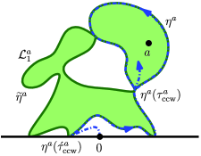
Let $\tau_{\mathrm{ccw}}^{a}\equiv\inf\{t\geq 0\dvtx\theta^{a}_{t}=2\pi\}$, the first time $\eta^{a}$ forms a counterclockwise loop surrounding $a$.

If $\tau_{\mathrm{ccw}}^{a}=\infty$, then there are no loops surrounding $a$ and we set $\mathcal{L}^{a}$ to be the empty sequence. If $\tau_{\mathrm{ccw}}^{a}<\infty$ let $\acute{\tau}_{\mathrm{ccw}}^{a}\equiv\sup\{t<\tau_{\mathrm{ccw}}^{a}\dvtx\theta^{a}_{t}=0\}$, let $o^{a}\equiv\eta^{a}(\acute{\tau}_{\mathrm{ccw}}^{a})$, and let $\widetilde{\eta}^{a}$ be the branch $\eta^{o^{a}}$, reparametrized so that $\widetilde{\eta}^{a}|_{[0,\tau_{\mathrm{ccw}}^{a}]}=\eta^{a}|_{[0,\tau_{\mathrm{ccw}}^{a}]}$. The outermost loop $\mathcal{L}^{a}_{1}$ surrounding $a$ is defined to be $\widetilde{\eta}^{a}|_{[\acute{\tau}_{\mathrm{ccw}}^{a},\infty]}$.

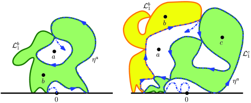
If $\mathcal{L}^{a}_{1}$ is defined, it is necessarily counterclockwise and pinned at $\eta^{a}(\acute{\tau}_{\mathrm{ccw}}^{a})$, and for any point $b$ surrounded by $\mathcal{L}^{a}_{1}$ we have $\mathcal{L}^{b}_{1}=\mathcal{L}^{a}_{1}$. Moreover, $\eta^{a}(\acute{\tau}_{\mathrm{ccw}}^{a})$ lies on $\partial\mathbb{D}$ if and only if $\eta^{a}$ has not previously made a clockwise loop around $a$ MR2494457 , Lemma 5.2. The next loop $\mathcal{L}^{a}_{2}$ surrounding $a$ is then defined in analogous fashion, and continuing in this way gives the full $\mathrm{CLE}_{\kappa}$ process $\Gamma$ in $\mathbb{D}$. See Figures 3 and 4.

Figure 3: Branching $\mathrm{SLE}_{\kappa}(\kappa-6)$ construction of $\mathrm{CLE}_{\kappa}$ ($4<\kappa<8$) process $\Gamma$ in $\mathbb{H}$. For each $a\in\mathbb{H}$, $\eta^{a}$ (dashed blue line) is the branch of the exploration tree targeted at $a$. It evolves as a radial $\mathrm{SLE}_{\kappa}(\kappa-6)$ which, whenever it hits the domain boundary or its past hull, continues in the complementary connected component containing $a$. Let $\tau_{\mathrm{ccw}}^{a}$ be the first time $t$ that $\eta^{a}$ completes a counterclockwise loop surrounding $a$; the location of the force point at time $\tau_{\mathrm{ccw}}^{a}$ is $o^{a}\equiv\eta^{a}(\acute{\tau}_{\mathrm{ccw}}^{a})$ for some $\acute{\tau}_{\mathrm{ccw}}^{a}<\tau_{\mathrm{ccw}}^{a}$. The outermost loop $\mathcal{L}_{1}^{a}$ of $\Gamma$ containing $a$ is $\eta^{o^{a}}|_{[\acute{\tau}_{\mathrm{ccw}}^{a},\infty]}$. Successive loops are defined in analogous fashion. $\mathcal{L}^{a}_{1}$ is necessarily counterclockwise and pinned at $\eta^{a}(\acute{\tau}_{\mathrm{ccw}}^{a})$. It is disjoint from the domain boundary if and only if $a$ is first surrounded by a clockwise loop.

Figure 4: Clockwise loops of $\eta^{a}$ (dashed blue line) are not $\mathrm{CLE}$ loops, but correspond either to complementary connected components of $\mathrm{CLE}$ loops (left panel) or complementary connected components of chains of $\mathrm{CLE}$ loops (right panel). The $\mathrm{CLE}$ process is renewed within each clockwise loop (Proposition 2.3).

Remark 2.2.

For $4<\kappa<8$, assuming the conjecture that chordal$\mathrm{SLE}_{\kappa}(\kappa-6)$ processes are generated by continuous curves with reversible law MR2494457 , Conjecture 3.11, it was shown MR2494457 , Proposition 5.1 and Theorem 5.4, that $\mathrm{CLE}_{\kappa}$ loops are continuous, and that the law of the full ensemble is independent of the choice of root for the exploration tree. This conjecture was proved in works of Miller and Sheffield (MSIMAG , Theorem 1.3 and MSIMAG3 , Theorems 1.1 and 1.2), so these properties hold. (The analogous continuity and root-invariance statements are immediate for $\kappa\in[8/3,4]$ by the equivalence of $\mathrm{CLE}_{\kappa}$ and the outer boundaries of loop soups SWCLE ; see also werner-wucle-exploration .)

The $\mathrm{CLE}_{\kappa}$ process in a general proper simply connected domain is defined by conformal transformation, so the law of $\mathrm{CLE}_{\kappa}$ is conformally invariant. Moreover, conditional on the collection of all of the outermost loops, the law of the loops contained in the connected component $D^{a}$ of $\mathbb{D}\setminus\mathcal{L}_{1}^{a}$ containing $a$ is equal to that of a $\mathrm{CLE}_{\kappa}$ in $D^{a}$ independently of the loops of $\Gamma$ which are not contained in $D^{a}$. The key observation which we use to prove Theorem 1.1 is that there are additional sources of conditional independence in $\mathrm{CLE}_{\kappa}$ when $\kappa>4$, in particular:

Proposition 2.3

Suppose $z\in D$ is surrounded by a clockwise loop $\mathcal{C}$ in the $\mathrm{SLE}_{\kappa}(\kappa-6)$ exploration tree of $D$ (as in Figure 4), allowing the domain boundary to form part of the loop $\mathcal{C}$. If $U$ is the connected component of $D\setminus\mathcal{C}$ containing $z$, then the law of the $\mathrm{CLE}_{\kappa}$ loops contained within $\overline{U}$ is that of a $\mathrm{CLE}_{\kappa}$ in $U$, independent of the $\mathrm{CLE}_{\kappa}$ loops outside of $U$.

The $\mathrm{SLE}_{\kappa}(\kappa-6)$ exploration tree for $\kappa>4$ has such clockwise loops, which are not $\mathrm{CLE}$ loops, and so provide additional renewal events.

2.3 Diffusion estimate

Proposition 2.4 ((MR2491617 , equation (4)))

Suppose $8/3<\kappa<8$, and let $\theta_{t}$ be the process defined above started from $\theta_{0}=0$, evolving according to SDE (4) in $(0,2\pi)$ and instantaneously reflecting at the endpoints $\{0,2\pi\}$. Then $\mathbb{P}[\theta_{s}<2\pi\ \forall s\leq t]\asymp e^{-\alpha t}$ where

$$\alpha\equiv\frac{(8-\kappa)(3\kappa-8)}{32\kappa}.$$ (6)

It is this diffusion exponent $\alpha$ which gave rise to the result of MR2491617 that the gasket has expectation dimension $2-\alpha$, implying an upper bound of $2-\alpha$ for the Hausdorff dimension, for which Theorem 1.1 provides the matching lower bound. The actual value of $\alpha$ does not play a significant role in the proof of Theorem 1.1, except that we use $0<\alpha<2$. (Of course, $\alpha\leq 2$ is a necessary condition for showing that the Hausdorff dimension is $2-\alpha$.)

2.4 Distortion estimates

For a proper simply connected domain $D$ and $w\in D$, let $\operatorname{CR}(w,D)$ denote the conformal radius of $D$ with respect to $w$, that is, $\operatorname{CR}(w,D)\equiv f^{\prime}(0)$ for $f$ the unique conformal map $\mathbb{D}\to D$ with $f(0)=w$ and $f^{\prime}(0)>0$. Let $\operatorname{rad}(w,D)\equiv\inf\{r\dvtx B_{r}(w)\supseteq D\}$ denote the out-radius of $D$ with respect to $w$. By the Schwarz lemma and the Koebe one-quarter theorem,

$$\operatorname{dist}(w,\partial D)\leq\operatorname{CR}(w,D)\leq\bigl{[}4\operatorname{dist}(w,\partial D)\bigr{]}\wedge\operatorname{rad}(w,D).$$ (7)

Further (see, e.g., MR1217706 , Theorem 1.3)

$$\frac{|\zeta|}{(1+|\zeta|)^{2}}\leq\frac{|f(\zeta)-w|}{\operatorname{CR}(w,D)}\leq\frac{|\zeta|}{(1-|\zeta|)^{2}}.$$

As a consequence,

$$\frac{|\zeta|}{4}\leq\frac{|f(\zeta)-w|}{\operatorname{CR}(w,D)}\leq 4|\zeta|,$$ (8)

where the right-hand inequality holds for $|\zeta|\leq 1/2$.

3 Proofs

Recall that a $\mathrm{CLE}_{\kappa}$ process in a general simply connected domain $D$ is defined as the image under a conformal transformation $f\dvtx\mathbb{D}\to D$ of a $\mathrm{CLE}_{\kappa}$ process $\Gamma$ in $\mathbb{D}$. Since $f|_{r\mathbb{D}}$ for any $0<r<1$ is bi-Lipschitz and so preserves Hausdorff dimension, and the Hausdorff dimension of a countable union is the supremum of the Hausdorff dimensions, we see that $f$ preserves Hausdorff dimension, and so it suffices to prove Theorem 1.1 with $D=\mathbb{D}$. Thus, for the remainder $\Gamma$ denotes a $\mathrm{CLE}_{\kappa}$ ($4<\kappa<8$) process on $\mathbb{D}$, constructed from the collection of radial $\mathrm{SLE}_{\kappa}(\kappa-6)$ curves $(\eta^{z})_{z\in\mathbb{D}}$ jointly defined on a probability space $(\Omega,\mathcal{F},\mathbb{P})$, as given by the remark following Proposition 2.1. In Section 3.1, we define our multi-scale refinement of the gasket $\mathcal{G}$ of $\Gamma$, and state the main result of the section, the second moment estimate Lemma 3.1 on the correlation structure of the set of “perfect points” identified by the refinement. We then use the $\mathrm{CLE}$ renewal property of Proposition 2.3 to reduce Lemma 3.1 to a lower bound on the probability of a single event. This bound is given by Proposition 3.3, which we prove in Section 3.2. The Hausdorff dimension lower bound follows from Lemma 3.1 by standard arguments which we give in Section 3.3, thereby concluding the proof of Theorem 1.1.

Figure 5: A single level of the multi-scale argument we use to prove the lower bound of Theorem 1.1. The curve $\eta$ (dashed blue line) is a radial $\mathrm{SLE}_{\kappa}(\kappa-6)$ targeted at zero. For $\beta>0$, $E(\eta)$ is the event that the first time $\tau_{\mathrm{cw}}$ that $\eta$ closes a clockwise loop $\mathcal{C}$ surrounding $0$ with $\mathcal{C}\subset e^{-\beta}\mathbb{D}$ is finite, and further that $\eta$ makes no counterclockwise loop surrounding $0$ before $\tau_{\mathrm{cw}}$. On the event $E(\eta)$, set $D(\eta)$ (light blue region) to be the connected component of $\mathbb{D}\setminus\eta[0,\tau_{\mathrm{cw}}]$ containing $0$.

3.1 Clockwise loops in small disks

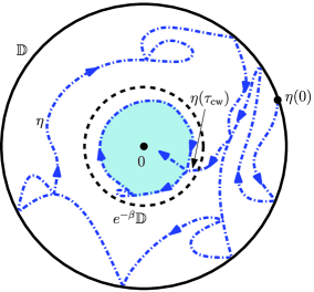
We now describe our multi-scale refinement of the gasket $\mathcal{G}$ which identifies a subset of “perfect points” (following the terminology of MR2123929 , MR2642894 ) in $\mathcal{G}$, satisfying a certain restriction at all scales which makes their correlation structure easy to analyze. Let $\beta>0$ be a parameter (which we will send to $\infty$). Let $\eta$ be any curve defined on $(\Omega,\mathcal{F},\mathbb{P})$ and traveling in $\overline{\mathbb{D}}$ from $\partial\mathbb{D}$ to $0$. For any curve $\eta$ defined on $(\Omega,\mathcal{F},\mathbb{P})$ and traveling in $\overline{\mathbb{D}}$ from $\partial\mathbb{D}$ to $0$, define $E(\eta)\subseteq\Omega$ to be the event that [(ii)]

the first time $\tau_{\mathrm{cw}}$ that $\eta$ closes a clockwise loop $\mathcal{C}$ surrounding $0$ with $\mathcal{C}\subset e^{-\beta}\mathbb{D}$ is finite; and

$\eta$ makes no counterclockwise loop surrounding $0$ before time $\tau_{\mathrm{cw}}$. On the event $E(\eta)$, set $D(\eta)$ to be the connected component of $\mathbb{D}\setminus\mathcal{C}$ containing the origin. See Figure 5 for an illustration.

We then define events $E_{j}$ and domains $D_{j}\ni 0$, both nonincreasing in $j$ for $j\geq 0$, as follows: let $(E_{0},D_{0})\equiv(\Omega,\mathbb{D})$, and suppose inductively that $(E_{j},D_{j})$ has been defined. Let $\mathsf{g}_{j}$ be the uniformizing map $D_{j}\to\mathbb{D}$ with $\mathsf{g}_{j}(0)=0$ and $\mathsf{g}_{j}^{\prime}(0)>0$, and let

$$\tau_{j}\equiv\inf\bigl{\{}t\geq 0\dvtx\eta(t)\in D_{j}\bigr{\}},\qquad\mathsf{g}_{j}\eta\equiv\bigl{(}\mathsf{g}_{j}\eta(\tau_{j}+s)\bigr{)}_{s\geq 0}.$$

We then set

$$E_{j+1}(\eta)\equiv E_{j}(\eta)\cap E(\mathsf{g}_{j}\eta),\qquad D_{j+1}(\eta)\equiv\mathsf{g}_{j}^{-1}D(\mathsf{g}_{j}\eta).$$

For $z\in\mathbb{D}$, let

$$\psi(\zeta)\equiv\psi_{z}(\zeta)\equiv\frac{\zeta-z}{1-\bar{z}\zeta},$$

the conformal automorphism of $\mathbb{D}$ with $\psi(z)=0$ and $\psi^{\prime}(z)=(1-|z|^{2})^{-1}>0$. For $\eta^{z}$, the branch of the $\mathrm{SLE}_{\kappa}(\kappa-6)$ exploration tree targeted at $z$, we set

$$E^{z}_{j}\equiv E_{j}\bigl{(}\psi_{z}\eta^{z}\bigr{)},\qquad D^{z}_{j}\equiv\psi_{z}^{-1}D_{j}\bigl{(}\psi_{z}\eta^{z}\bigr{)}.$$ (9)

The perfect points in the multi-scale refinement of the gasket $\mathcal{G}$ are the points $z\in\mathbb{D}$ for which $\bigcap_{j\geq 0}E^{z}_{j}$ occurs. The main estimate needed to lower bound the Hausdorff dimension is the following estimate on their correlation structure.

Lemma 3.1

For sufficiently large $\beta$ there exists $\varepsilon\equiv\varepsilon(\beta)<\infty$ with $\lim_{\beta\to\infty}\varepsilon(\beta)=0$ such that for all $z,w\in\mathbb{D}$,

$$\frac{\mathbb{P}[E^{z}_{n}\cap E^{w}_{n}]}{\mathbb{P}[E^{z}_{n}]\mathbb{P}[E^{w}_{n}]}\leq\biggl{(}\frac{e^{\beta}}{|z-w|}\biggr{)}^{\alpha(1+\varepsilon)},$$

where $\alpha$ is given by (6).

In the remainder of this subsection, we reduce the proof of this lemma to a lower bound on the probability of the event $E^{0}_{1}$, Proposition 3.3, which we prove in Section 3.2. We begin with some easy estimates comparing the domains $D^{z}_{j}$ to disks $B_{e^{-j\beta}}(z)$.

Lemma 3.2

For $\beta\geq\log 2$, $j\geq 1$, and $z\in\mathbb{D}$,

$$\operatorname{rad}\bigl{(}z,D^{z}_{j}\bigr{)}\leq 8e^{-j\beta}\qquad\mbox{on }E^{z}_{j}.$$ (10)

We first consider the domains $D_{j}\equiv D_{j}(\eta)$, defined on the event $E_{j}(\eta)$, for any curve $\eta$ traveling in $\overline{\mathbb{D}}$ from $\partial\mathbb{D}$ to $0$. [We will later take $\eta=\psi_{z}(\eta^{z})$, where $\eta^{z}$ is the branch of the $\mathrm{SLE}_{\kappa}(\kappa-6)$ exploration tree targeted at $z$, and $\psi_{z}$ is the Möbius transformation defined above which maps $z$ to $0$.] Recall the definition of the uniformizing map $\mathsf{g}_{j}\dvtx D_{j}\to\mathbb{D}$. By the definition of $D_{j}$ and by (7),

$$\operatorname{CR}(0,\mathsf{g}_{j-1}D_{j})\leq\operatorname{rad}(0,\mathsf{g}_{j-1}D_{j})\leq e^{-\beta}.$$ (11)

Since

$$\operatorname{CR}(0,\mathsf{g}_{j-1}D_{j})=\frac{1}{(\mathsf{g}_{j}\circ\mathsf{g}_{j-1}^{-1})^{\prime}(0)}=\frac{\operatorname{CR}(0,D_{j})}{\operatorname{CR}(0,D_{j-1})},$$

we have that

$$\operatorname{CR}(0,D_{j})=\prod_{\ell=1}^{j}\operatorname{CR}(0,g_{\ell-1}D_{\ell})\leq e^{-j\beta}.$$ (12)

Applying the right-hand inequality of (8) with $f=\mathsf{g}_{j-1}^{-1}$ gives

$$\frac{|\zeta|}{\operatorname{CR}(0,D_{j-1})}\leq 4\bigl{|}\mathsf{g}_{j-1}(\zeta)\bigr{|}\leq 4e^{-\beta}\qquad\mbox{when }\zeta\in\partial D_{j},$$

using that $\zeta\in\partial D_{j}$ implies $|\mathsf{g}_{j-1}(\zeta)|\leq e^{-\beta}\leq 1/2$. Rearranging and combining with (12) gives

$$|\zeta|\leq 4e^{-\beta}\operatorname{CR}(0,D_{j-1})\leq 4e^{-j\beta}\qquad\mbox{when }\zeta\in\partial D_{j}.$$ (13)

For any $z\in\mathbb{D}$, (13) is satisfied with $D_{j}=D_{j}(\psi_{z}\eta^{z})=\psi_{z}D^{z}_{j}$ on the event $E^{z}_{j}$. We have $\psi_{z}^{-1}(\zeta)=(z+\zeta)/(1+\bar{z}\zeta)$, so

$$\bigl{|}\psi_{z}^{-1}(\zeta)-z\bigr{|}=\biggl{|}\zeta\frac{1-|z|^{2}}{1+\bar{z}\zeta}\biggr{|}\leq|\zeta|\frac{1-|z|^{2}}{1-|z|}=|\zeta|\bigl{(}1+|z|\bigr{)}\leq 2|\zeta|,$$

giving $\operatorname{rad}(z,D^{z}_{j})\leq 2\operatorname{rad}(0,\psi_{z}D^{z}_{j})\leq 8e^{-j\beta}$ as claimed.

Let $\mathcal{F}^{z}_{j}$ denote the $\sigma$-algebra generated by $\eta^{z}$ up to the time $\tau^{z}_{j}$ that $\eta^{z}$ closes the clockwise loop forming the boundary of $D^{z}_{j}$ (if $E^{z}_{j}$ does not occur then $\tau^{z}_{j}=\infty$). By the conformal Markov property of radial $\mathrm{SLE}_{\kappa}(\rho)$, for $m\leq n$, we have

$$\mathbb{P}\bigl{[}E^{z}_{n}|\mathcal{F}_{m}^{z}\bigr{]}\mathbf{1}_{E^{z}_{m}}=\mathbb{P}\bigl{[}E^{z}_{n-m}\bigr{]}\mathbf{1}_{E^{z}_{m}}=\mathbb{P}\bigl{[}E^{0}_{n-m}\bigr{]}\mathbf{1}_{E^{z}_{m}},$$

and consequently

$$\mathbb{P}\bigl{[}E^{z}_{n}\bigr{]}=\mathbb{E}\bigl{[}\mathbb{P}\bigl{[}E^{z}_{n}|\mathcal{F}_{n-1}^{z}\bigr{]}\mathbf{1}_{E^{z}_{n-1}}\bigr{]}=\mathbb{P}\bigl{[}E^{0}_{1}\bigr{]}\mathbb{P}\bigl{[}E^{z}_{n-1}\bigr{]}=\cdots=\mathbb{P}\bigl{[}E^{0}_{1}\bigr{]}^{n}.$$

Proposition 3.3

There exists a constant $c>0$ such that $\mathbb{P}[E^{0}_{1}]\geq(ce^{\alpha\beta})^{-1}$ for sufficiently large $\beta$, where $\alpha$ is given by (6).

The proof of this proposition is deferred to Section 3.2, but we show now how to use it to deduce Lemma 3.1.

Proof of Lemma 3.1 Given $z,w\in\mathbb{D}$, let $m\in\mathbb{N}$ be defined by $8e^{-m\beta}<|z-w|\leq 8e^{-(m-1)\beta}$. If $E^{z}_{m}\cap E^{w}_{m}$ occurs, then Lemma 3.2 implies $w\notin D_{m}^{z}$ which in turn implies $D_{m}^{z}\cap D_{m}^{w}=\varnothing$. So for $n\geq m$, $E^{z}_{n}$ and $E^{w}_{n}$ are conditionally independent given $E^{z}_{m}\cap E^{w}_{m}$, and in fact

$$\mathbb{P}\bigl{[}E^{z}_{n}\cap E^{w}_{n}|E^{z}_{m}\cap E^{w}_{m}\bigr{]}=\mathbb{P}\bigl{[}E^{0}_{n-m}\bigr{]}^{2}.$$

Therefore

$$\mathbb{P}\bigl{[}E^{z}_{n}\cap E^{w}_{n}\bigr{]} = \mathbb{P}\bigl{[}E^{z}_{m}\cap E^{w}_{m}\bigr{]}\mathbb{P}\bigl{[}E^{0}_{n-m}\bigr{]}^{2}$$

$$\leq \frac{(\mathbb{P}[E^{0}_{m}]\mathbb{P}[E^{0}_{n-m}])^{2}}{\mathbb{P}[E^{0}_{m}]}=\frac{\mathbb{P}[E^{0}_{n}]^{2}}{\mathbb{P}[E^{0}_{1}]^{m}}\leq\bigl{(}ce^{\alpha\beta}\bigr{)}^{m}\mathbb{P}\bigl{[}E^{0}_{n}\bigr{]}^{2},$$

where the last inequality is by Proposition 3.3. But $|z-w|\leq 8e^{-(m-1)\beta}$ implies

$$m\beta\leq\beta+\log\frac{8}{|z-w|},$$

therefore

$$\log\biggl{(}\frac{\mathbb{P}[E^{z}_{n}\cap E^{w}_{n}]}{\mathbb{P}[E^{0}_{n}]^{2}}\biggr{)}\leq\alpha m\beta\biggl{(}1+\frac{\log c}{\alpha\beta}\biggr{)}\leq\alpha\bigl{(}1+O(1/\beta)\bigr{)}\biggl{[}\beta+\log\frac{1}{|z-w|}\biggr{]}.$$

As $\beta\to\infty$, the error term goes to $0$, which implies the result.

3.2 Probability of a clockwise loop

In this section, we prove Proposition 3.3, lower bounding the probability that a radial $\mathrm{SLE}_{\kappa}(\kappa-6)$ process in $\mathbb{D}$ makes a clockwise loop within the disk $e^{-\beta}\mathbb{D}$ before making any counterclockwise loop surrounding the origin.

Some notation: for $x\in[0,2\pi]$, we write $\theta^{(x)}_{t}$ for the $[0,2\pi]$-valued process of Section 2.1 started from $\theta^{(x)}_{0}=x$, evolving according to SDE (4) in $(0,2\pi)$ and instantaneously reflecting at the endpoints $\{0,2\pi\}$. We write $\theta_{t}\equiv\theta^{(0)}_{t}$, and for $a\in[0,2\pi]$ we let $\sigma_{a}\equiv\inf\{t\dvtx\theta_{t}=a\}$, and set $F_{t}\equiv\{\sigma_{2\pi}>t\}$. For $0<R<1$ and $\theta_{0}\in[0,2\pi]$ let $P_{R}(\theta_{0})$ be the probability that a radial $\mathrm{SLE}_{\kappa}(\kappa-6)$ in $\mathbb{D}$ with starting configuration $(w,o)=(1,e^{-i\theta_{0}})$ and target $0$ makes a clockwise loop inside the disk $R\mathbb{D}$ surrounding $0$ before making any counterclockwise loop surrounding $0$. The proposition will be obtained from the following two lemmas, whose proof we defer.

Lemma 3.4

There exist $c_{0},p_{0}>0$ such that

$$\mathbb{P}\bigl{[}\theta_{T}\in[c_{0},2\pi-c_{0}]|F_{T}\bigr{]}\geq p_{0}\qquad\mbox{for all }T\in[1,\infty).$$

Lemma 3.5

For any $c_{0}>0$, we have $\inf_{\theta_{0}\in[c_{0},2\pi-c_{0}]}P_{R}(\theta_{0})>0$.

Proof of Proposition 3.3 Recall that it is natural to parametrize the radial $\mathrm{SLE}_{\kappa}(\kappa-6)$ curve $\eta^{0}$ targeted at $0$ by capacity: if $U_{t}$ denotes the unique connected component of $\mathbb{D}\setminus\eta^{0}[0,t]$ containing $0$ and $g_{t}$ is the unique conformal transformation $U_{t}\to\mathbb{D}$ with $g_{t}(0)=0$ and $g_{t}^{\prime}(0)>0$, then $g_{t}^{\prime}(0)=1/\operatorname{CR}(0,U_{t})=e^{t}$.

Assume $\beta\geq\log 8$, and let $\beta^{\prime}\equiv\beta-\log 8\geq 0$. Consider the map $g_{\beta^{\prime}}\dvtx U_{\beta^{\prime}}\to\mathbb{D}$. The left-hand inequality of (8) with $f=g_{\beta^{\prime}}^{-1}$ gives $|g_{\beta^{\prime}}(\zeta)|\leq 4|\zeta|e^{\beta^{\prime}}$ for any $\zeta\in U_{\beta^{\prime}}$. In particular, $|g_{\beta^{\prime}}(\zeta)|\leq 1/2$ for $|\zeta|\leq e^{-\beta^{\prime}}/8=e^{-\beta}$, so we can apply the right-hand inequality of (8) to find

$$e^{\beta^{\prime}}|\zeta|\leq 4\bigl{|}g_{\beta^{\prime}}(\zeta)\bigr{|}\qquad\mbox{when }|\zeta|\leq e^{-\beta}.$$

Therefore, the image of $e^{-\beta}\mathbb{D}$ under $g_{\beta^{\prime}}$ contains $R\mathbb{D}$ where

$$R=\tfrac{1}{4}e^{\beta^{\prime}-\beta}=\tfrac{1}{32}.$$

The curve $g_{\beta^{\prime}}\eta^{0}$ is distributed as an $\mathrm{SLE}_{\kappa}(\kappa-6)$ in $\mathbb{D}$ with starting configuration $(\tilde{W}_{0},\tilde{O}_{0})=(W_{\beta^{\prime}},W_{\beta^{\prime}}e^{-i\theta_{\beta^{\prime}}})$, so for any $c>0$ we have

$$\mathbb{P}\bigl{[}E_{1}^{0}\bigr{]}\geq\mathbb{P}[F_{\beta^{\prime}}]\mathbb{P}\bigl{[}\theta_{\beta^{\prime}}\in[c,2\pi-c]|F_{\beta^{\prime}}\bigr{]}\inf_{\theta_{0}\in[c,2\pi-c]}P_{R}(\theta_{0}).$$

By Proposition 2.4, Lemmas 3.4 and 3.5 this expression is $\asymp e^{-\alpha\beta^{\prime}}$, which gives the result.

The remainder of this subsection is devoted to proving the above lemmas. We will obtain Lemma 3.4 as a consequence of the following lemma.

Lemma 3.6

For any deterministic time $T\geq 0$,

$$\mathbb{P}[\theta_{T}\leq\pi|F_{T}]\geq 1/2.$$

Let $S=\pm 1$ be a symmetric random sign independent of the process $\theta_{t}$, and consider the event $A_{T}\equiv\{\theta_{T}<\pi\}\cup\{\theta_{T}=\pi,S=1\}$. (The random sign is introduced to handle the possibility that $\theta_{T}=\pi$. It follows easily by comparison with Bessel processes, see, for example, the proof of Lemma 3.4, that $\mathbb{P}[F_{T}]>0$ and $\mathbb{P}[\theta_{T}=\pi]=0$ for all deterministic $T\geq 0$, but our proof of Lemma 3.6 can be applied to any strong Markov continuous process with reflective symmetry.) By the strong Markov property of $\theta_{t}$ and the reflective symmetry across $\pi$ of its drift coefficient,

$$\mathbb{P}\bigl{[}A_{T}^{c}\bigr{]}=\mathbb{P}[\theta_{T}>\pi]+\tfrac 12\mathbb{P}[\theta_{T}=\pi]=\tfrac 12\mathbb{P}[\sigma_{\pi}\leq T,\theta_{T}\neq\pi]+\tfrac 12\mathbb{P}[\theta_{T}=\pi]\leq\tfrac 12.$$

By a similar argument $\mathbb{P}[A_{T}|F_{T}^{c}]\leq 1/2$. Since $\mathbb{P}[A_{T}]\geq 1/2$ is a weighted average of $\mathbb{P}[A_{T}|F_{T}^{c}]\leq 1/2$ and $\mathbb{P}[A_{T}|F_{T}]$, we conclude $\mathbb{P}[A_{T}|F_{T}]\geq 1/2$, which implies the lemma.

Recall the notation $\theta^{(x)}_{t}$ defined above. Using the same driving Brownian motion for any countable collection of processes $\theta_{t}^{(x)}$ gives a coupling under which (by continuity and pathwise uniqueness) the relative order among the processes is preserved over time.

Proof of Lemma 3.4 For $T\geq 1$ and $c_{0}\in(0,\pi)$, it follows from the Markov property and Lemma 3.6 that

$$\mathbb{P}[c_{0}\leq\theta_{T}\leq 3\pi/2|F_{T}] \geq \mathbb{P}[c_{0}\leq\theta_{T}\leq 3\pi/2,\theta_{T-1}\leq\pi|F_{T}]$$

$$\geq \frac{\mathbb{P}[\theta_{T-1}\leq\pi|F_{T-1}]\inf_{x\leq\pi}\mathbb{P}[c_{0}\leq\theta_{1}^{(x)}\leq 3\pi/2,F_{1}^{(x)}]}{\mathbb{P}[F_{T}|F_{T-1}]}$$

$$\geq \frac{1}{2}\inf_{x\leq\pi}\mathbb{P}\bigl{[}\theta_{1}^{(x)}\in[c_{0},3\pi/2],F_{1}^{(x)}\bigr{]}$$

$$\geq \frac{1}{2}\mathbb{P}\Bigl{[}\theta^{(0)}_{1}\geq c_{0},\max_{t\leq 1}\theta^{(\pi)}_{t}\leq 3\pi/2\Bigr{]},$$

where the last line follows by the coupling described above. Recall SDE (4); since $\cot(y/2)/2\sim 1/y$ as $y\downarrow 0$, by Girsanov’s theorem the process $\theta^{(x)}_{t}$ before hitting $3\pi/2$ has law mutually absolutely continuous with respect to that of a $\sqrt{\kappa}\mathrm{\textsc{bes}}^{\delta}$ process ($\sqrt{\kappa}$ times a $\delta$-dimensional Bessel process) started from $x$, with $\delta\equiv 1+2(\kappa-4)/\kappa$. Note that $\delta>0$ since $\kappa>8/3$. A $\sqrt{\kappa}\mathrm{\textsc{bes}}^{\delta}$ process started from $x\leq\pi$ has positive probability not to hit $3\pi/2$ by time $T$, so $\mathbb{P}[\max_{t\leq 1}\theta^{(\pi)}_{t}\leq 3\pi/2]>0$. Meanwhile the process $\theta^{(0)}_{t}$ before hitting $2\pi$ is mutually absolutely continuous with respect to another $\sqrt{\kappa}\mathrm{\textsc{bes}}^{\delta}$ process (started from zero), so in particular the random variable $\theta^{(0)}_{1}$ does not have an atom at $0$ on the event $\{\max_{t\leq 1}\theta^{(\pi)}_{t}\leq 3\pi/2\}$. Therefore

$$\lim_{c_{0}\downarrow 0}\mathbb{P}\Bigl{[}\theta^{(0)}_{1}\geq c_{0},\max_{t\leq 1}\theta^{(\pi)}_{t}\leq 3\pi/2\Bigr{]}=\mathbb{P}\Bigl{[}\max_{t\leq 1}\theta^{(\pi)}_{t}\leq 3\pi/2\Bigr{]}>0,$$

which proves the existence of $c_{0},p_{0}>0$ such that $\mathbb{P}[\theta_{T}\in[c_{0},2\pi-c_{0}]|F_{T}]\geq p_{0}$ for all $T\geq 1$.

Proof of Lemma 3.5 Throughout the proof, let $\eta\equiv\eta_{\theta_{0}}$ denote a radial $\mathrm{SLE}_{\kappa}(\kappa-6)$ process in $\mathbb{D}$ with starting configuration $(1,e^{-i\theta_{0}})$ and target $0$.

We begin by comparing nearby values of $\theta_{0}$. Let $o=e^{i\theta_{0}}$ and $o^{\prime}=e^{i\theta_{0}^{\prime}}$, where $0<\theta_{0},\theta_{0}^{\prime}<2\pi$. The Möbius transformation

$$f_{oo^{\prime}}(\zeta)\equiv\frac{o^{\prime}}{o}\frac{(o+\bar{o}^{\prime}-2)\zeta+(1-o\bar{o}^{\prime})}{(\bar{o}+o^{\prime}-2)+(1-\bar{o}o^{\prime})\zeta}=\zeta+\frac{(o^{\prime}-o)(\zeta-1)^{2}}{(1-2o+oo^{\prime})+(o-o^{\prime})\zeta}$$

is the automorphism of $\mathbb{D}$ sending $1$ to $1$, $o$ to $o^{\prime}$, and $\bar{o}^{\prime}$ to $\bar{o}$. Suppose $\theta_{0},\theta_{0}^{\prime}\in[c_{0},2\pi-c_{0}]$. Then $|1-2o+oo^{\prime}|=|2-\bar{o}-o^{\prime}|$ is at least $2-\operatorname{Re}(o+o^{\prime})\geq 2(1-\cos c_{0})$, thus bounded away from $0$. From this, it is clear that if $|\theta_{0}-\theta_{0}^{\prime}|$ is sufficiently small, then the image of $R\mathbb{D}$ under $f_{oo^{\prime}}$ will contain the disk $(R-\varepsilon)\mathbb{D}$. It follows that $P_{R}(\theta_{0})\geq P_{R-\varepsilon}(\theta_{0}^{\prime})$ [using the target invariance of Proposition 2.1 since $f_{oo^{\prime}}(\eta_{\theta_{0}})$ has target $f_{oo^{\prime}}(0)\neq 0$]. This reduces the problem of showing $\inf_{\theta_{0}\in[c_{0},2\pi-c_{0}]}P_{R}(\theta_{0})>0$ to that of showing $P_{R}(\theta_{0})>0$ for each fixed choice of $0<R<1$ and $\theta_{0}\in[c_{0},2\pi-c_{0}]$.

We prove $P_{R}(\theta_{0})>0$ in two steps which are informally explained in Figures 6 and 7.

Figure 6: Proof of Lemma 3.5, Step 1: almost clockwise loop. A radial $\mathrm{SLE}_{\kappa}(\kappa-6)$ curve $\eta$ (dashed blue line) with starting configuration $(w,o)=(1,e^{-i\theta_{0}})$ ($\theta_{0}\in[c_{0},2\pi-c_{0}]$) evolves as ordinary chordal $\mathrm{SLE}_{\kappa}$ from $w$ to $o$, with (chordal) driving function $W^{\prime}$ which is $\sqrt{\kappa}$ times a standard Brownian motion. Therefore, $W^{\prime}$ has positive probability to be uniformly close to the driving function $W^{\star}$ of the hook curve $\eta^{\star}$. On this event, $\eta$ is close to $\eta^{\star}$ in Hausdorff distance and therefore forms an almost clockwise loop. Write $U$ for the complementary connected component of the path of $\eta$ so far which contains $z^{\delta}$. That $\eta$ closes the clockwise loop with positive probability is explained in Figure 7.

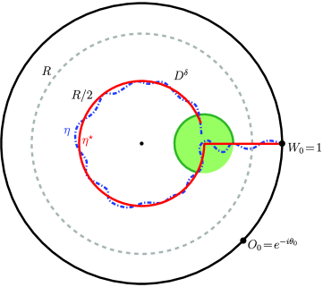
Step 1: Almost clockwise loop. The function

$$f(\zeta)=\frac{i(\zeta-1)(o-1)}{2(\zeta-o)},$$

conformally maps $\mathbb{D}$ to $\mathbb{H}$ sending $W_{0}=1$ to $0$ and $O_{0}=o$ to $\infty$. Observe

$$\bigl{|}f^{\prime}(\zeta)\bigr{|}=\biggl{|}-\frac{i(o-1)^{2}}{2(\zeta-o)^{2}}\biggr{|}\geq\frac{|o^{1/2}-o^{-1/2}|^{2}}{8}\geq\frac{\sin^{2}(c_{0}/2)}{2}\qquad\mbox{for }\zeta\in\mathbb{D},$$

so the inverse transformation $f^{-1}\dvtx\mathbb{H}\to\mathbb{D}$ is Lipschitz.

Recall from Section 2.1 that up to the stopping time $\tau_{=}\equiv\inf\{t\geq 0\dvtx W_{t}=O_{t}\}$, $\eta$ coincides (modulo time change) with the exploration tree branch $\eta^{o}$, which is an ordinary chordal $\mathrm{SLE}_{\kappa}$ in $\mathbb{D}$ from $W_{0}=1$ to $O_{0}=o$. That is, $f(\eta^{o}(u))_{u\geq 0}$ is a standard chordal $\mathrm{SLE}_{\kappa}$ in $\mathbb{H}$ with associated chordal Loewner driving function $W^{\prime}_{u}=\sqrt{\kappa}B_{u}$ for $B_{u}$ a standard Brownian motion, and $\eta(t(u))=\eta^{o}(u)$ for $t(u)\leq\tau_{=}$.

Figure 7: Proof of Lemma 3.5, Step 2: loop closure. The left panel shows $U$ in a neighborhood of $z^{\delta}$ (see Figure 6 for the notation). The right panel shows the image of $U$ under the conformal map $\varphi\dvtx U\to\mathbb{D}$ with $\varphi(z^{\delta})=0$, $\varphi^{\prime}(z^{\delta})>0$. By conformal invariance of Brownian motion, it follows from consideration of hitting probabilities of Brownian motion started from $z^{\delta}$ in Figure 6 that as $\delta\downarrow 0$, $\varphi(J_{\pm})$ converge to points on $\partial\mathbb{D}$ bounded away from one another, and from the image of the tip of $\eta$ under $\varphi$. Loop closure occurs if $\varphi(\eta)$ crosses to the opposing arc $\varphi(K_{\infty})$ before reaching $\varphi(O_{0})$; this has positive probability for sufficiently small $\delta$ since $\mathrm{SLE}_{\kappa}$ ($4<\kappa<8$) is boundary-intersecting but not boundary-filling.

For $0<\delta\ll c_{0}$, consider the curve $\eta^{\star}$ in $\mathbb{D}$ which travels in a straight line from $1$ to $R/2$, then travels clockwise along the circle $\{\zeta\dvtx|\zeta|=R/2\}$ until it reaches $z^{\delta}\equiv(R/2)e^{i\delta/2}$. Let $W^{\star}_{u}$ be the driving function for $f(\eta^{\star})$ viewed as a chordal Loewner evolution in $\mathbb{H}$, defined up to the half-plane capacity $T^{\star}<\infty$ of $f(\eta^{\star})$. By MR2129588 , Lemma 4.2, $W^{\star}_{u}$ is continuous in $u$, hence uniformly continuous on $[0,T^{\star}]$ and thus uniformly approximable by a piecewise linear function (with finitely many pieces). Since $W^{\prime}_{u}$ is a Brownian motion, for any $\delta^{\prime}>0$ the event

$$\sup_{u\leq T^{\star}}\bigl{|}W^{\prime}_{u}-W^{\star}_{u}\bigr{|}\leq\delta^{\prime}$$ (14)

occurs with positive probability. By MR2129588 , Proposition 4.47, there exists $\delta^{\prime}>0$ such that if (14) occurs, then $f(\eta^{o}[0,T^{\star}])$ is within Hausdorff distance $\delta^{2}\sin^{2}(c_{0}/2)/2$ of $f(\eta^{\star})$, so $\eta^{o}[0,T^{\star}]$ is within Hausdorff distance $\delta^{2}$ of $\eta^{\star}$. For sufficiently small $\delta$ this implies $t(T^{\star})<\tau_{=}$, therefore $\eta[0,t(T^{\star})]$ coincides with $\eta^{o}[0,T^{\star}]$. Thus, if we define stopping times

$$\sigma\equiv\inf\bigl{\{}t\geq 0\dvtx\arg\eta(t)=\delta\bigr{\}},\qquad\acute{\sigma}\equiv\inf\bigl{\{}t\geq 0\dvtx\operatorname{dist}\bigl{(}\eta(t),\eta^{\star}\bigr{)}\geq\delta^{2}\bigr{\}},$$

then we will have $\sigma<\acute{\sigma}$ on the event (14).

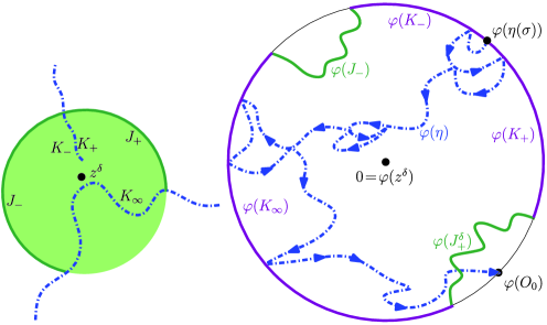
Step 2: Loop closure. On the event $\{\sigma<\acute{\sigma}\}$, let $\tau$ be the first time that $\eta$ closes a clockwise loop inside the disk $R\mathbb{D}$, and $\acute{\tau}$ the first time after $\sigma$ that $\eta$ exits $B_{R/4}(R/2)$; the result will follow by showing that

$$\liminf_{\delta\downarrow 0}\mathbb{P}[\tau<\acute{\tau}|\sigma<\acute{\sigma}]>0.$$ (15)

Let $U$ denote the unique connected component of $\mathbb{D}\setminus\eta[0,\sigma]$ whose closure contains both $0$ and $O_{0}$. Recall that $z^{\delta}\equiv(R/2)e^{i\delta/2}\in U$, and let $\varphi\equiv\varphi^{\delta}$ denote the uniformizing map $U\to\mathbb{D}$ with $\varphi(z^{\delta})=0$ and $\varphi^{\prime}(z^{\delta})>0$. Let $J_{+}$ (resp., $J_{-}$) denote the unique connected component of $U\cap\partial B_{R/4}(R/2)$ containing the point $(R/2)+e^{i\pi/4}(R/4)$ (resp., $R/4$): the $J_{\pm}$ are disjoint crosscuts of $U$, and we write $G$ for the connected component of $U\setminus(J_{+}\cup J_{-})$ containing $z^{\delta}$. The boundary $\partial G$ has a parametrization as a closed curve $b\dvtx[0,2\pi]\to\partial G$, oriented counterclockwise with $b(0)=b(2\pi)=\eta(\sigma)$. We then define times $0<t_{1}<t_{2}<t_{3}<t_{4}<2\pi$ such that $b(t_{1},t_{2})=J_{-}$ and $b(t_{3},t_{4})=J_{+}$, and write $K_{-}\equiv b[0,t_{1}]$, $K_{+}\equiv b[t_{4},2\pi]$, $K_{\infty}\equiv b[t_{2},t_{3}]$.

By the conformal Markov property, the probability of $\{\tau<\acute{\tau}\}$, conditioned on the path $\eta$ up to time $\sigma$ on the event $\{\sigma<\acute{\sigma}\}$, is given by the probability that a chordal $\mathrm{SLE}_{\kappa}$ traveling in $\mathbb{D}$ from $\varphi(\eta(\sigma))$ to $\varphi(O_{0})$ hits $\varphi(K_{\infty})$ before hitting $\varphi(J_{\pm})$. It follows from consideration of hitting probabilities of Brownian motion traveling in $U$ started from $z^{\delta}$ (using, e.g., the Beurling estimate MR2129588 , Theorem 3.76) that as $\delta\downarrow 0$, the diameters of the $\varphi(J_{\pm})$ tend to zero while the boundary arcs $\varphi(K_{\infty})$ and $\varphi(K_{\pm})$ are all of sizes bounded away from zero. Since $\mathrm{SLE}_{\kappa}$ ($4<\kappa<8$) is a.s. boundary-intersecting but not boundary-filling (see MR2129588 , Proposition 6.8) it follows that for sufficiently small $\delta$ this probability is positive.

3.3 Hausdorff dimension

In this section, we use the second moment estimate Lemma 3.1 and the lower bound Proposition 3.3 to deduce the main result Theorem. 1.1. The argument is standard (see, e.g., MR2642894 , Lemma 3.4) but we give some details here for completeness.

The $\gamma$-energy of a Borel measure $\mu$ on a metric space $(E,d)$ is

$$I_{\gamma}(\mu)=\int_{E}\int_{E}\,d(x,y)^{-\gamma}\,d\mu(x)\,d\mu(y).$$

If there exists a positive Borel measure on $E$ with finite $\gamma$-energy, then $E$ has Hausdorff dimension bounded below by $\gamma$ (see, e.g., MR2604525 , Theorem 4.27).

Proof of Theorem 1.1 Following the proof of MR2642894 , Lemma 3.4, we first show that for any fixed $\varepsilon>0$, there exists with positive probability a nonzero Borel measure supported on the $\mathrm{CLE}_{\kappa}$ gasket with finite $[2-\alpha(1+2\varepsilon)]$-energy, where $\alpha$ is given by (6).

For the full range of $\kappa$ we have $\alpha<2$, so we may assume $\varepsilon$ is sufficiently small that $\alpha(1+\varepsilon)<2$. Fix $\beta$ large such that $e^{\beta}/2$ is an integer and $\varepsilon(\beta)\leq\varepsilon$, with $\varepsilon(\beta)$ as in the statement of Lemma 3.1, and $c\leq e^{\varepsilon\alpha\beta}$, with $c$ as in the statement of Proposition 3.3.

For $z\in\mathbb{C}$ let $S_{r}(z)\equiv z+[-\frac{r}{2},\frac{r}{2})\times[-\frac{r}{2},\frac{r}{2})$ denote the box with side length $r$ centered at $z$, and write $H\equiv S_{1}(0)\subset\mathbb{D}$. For $n\geq 0$ let $S^{z}_{n}\equiv S_{e^{-n\beta}}(z)$. Since $e^{\beta}/2$ is an integer, $H$ can be expressed as the disjoint union

$$H=\bigsqcup_{z\in H_{n}}S^{z}_{n},\qquad H_{n}\equiv\bigl{\{}e^{-n\beta}(\mathbb{Z}+1/2)\bigr{\}}^{2}\cap H.$$

Recall the events $E_{n}^{z}$ defined in (9). Define a random measure $\mu_{n}$ on $H$ by

$$\mu_{n}(A)=\int_{A}\sum_{z\in H_{n}}\frac{\mathbf{1}\{E^{z}_{n}\}}{\mathbb{P}[E^{z}_{n}]}\mathbf{1}\bigl{\{}z^{\prime}\in S^{z}_{n}\bigr{\}}\,dz^{\prime},\qquad A\subseteq H.$$

Then $\mathbb{E}[\mu_{n}(H)]=1$, and

$$\mathbb{E}\bigl{[}\bigl{(}\mu_{n}(H)\bigr{)}^{2}\bigr{]}=e^{-4n\beta}\sum_{z,w\in H_{n}}\frac{\mathbb{P}[E^{z}_{n}\cap E^{w}_{n}]}{\mathbb{P}[E^{z}_{n}]\mathbb{P}[E^{w}_{n}]}.$$

The sum over off-diagonal terms is, by Lemma 3.1,

$$e^{-4n\beta}\mathop{\sum_{z,w\in H_{n}}}_{z\neq w}\frac{\mathbb{P}[E^{z}_{n}\cap E^{w}_{n}]}{\mathbb{P}[E^{z}_{n}]\mathbb{P}[E^{w}_{n}]}\leq e^{-2n\beta}e^{\alpha\beta(1+\varepsilon)}\mathop{\sum_{w\in(e^{-n\beta}\mathbb{Z})^{2}}}_{|w|<\sqrt{2}}\frac{1}{|w|^{\alpha(1+\varepsilon)}}\preccurlyeq e^{\alpha\beta(1+\varepsilon)},$$

using $\alpha(1+\varepsilon)<2$. By Proposition 3.3, the sum over diagonal terms is

$$e^{-4n\beta}\sum_{z\in H_{n}}\frac{1}{\mathbb{P}[E^{z}_{n}]}\leq e^{-2n\beta}\bigl{(}ce^{\alpha\beta}\bigr{)}^{n}\leq e^{-n\beta[2-\alpha(1+\varepsilon)]}\leq 1,$$

therefore $\mathbb{E}[\mu_{n}(H)^{2}]\preccurlyeq e^{\alpha\beta(1+\varepsilon)}$. Similarly,

$$\mathbb{E}\bigl{[}I_{2-\alpha(1+2\varepsilon)}(\mu_{n})\bigr{]}$$

$$\qquad=\sum_{z,w\in H_{n}}\frac{\mathbb{P}[E^{z}_{n}\cap E^{w}_{n}]}{\mathbb{P}[E^{z}_{n}]\mathbb{P}[E^{w}_{n}]}\int_{S^{z}_{n}}\int_{S^{w}_{n}}\frac{1}{|z^{\prime}-w^{\prime}|^{2-\alpha(1+2\varepsilon)}}\,dw^{\prime}\,dz^{\prime}$$

$$\qquad\preccurlyeq e^{-4n\beta}\sum_{z,w\in H_{n}}\frac{\mathbb{P}[E^{z}_{n}\cap E^{w}_{n}]}{\mathbb{P}[E^{z}_{n}]\mathbb{P}[E^{w}_{n}]}\biggl{\{}e^{n\beta[2-\alpha(1+2\varepsilon)]}\wedge\frac{1}{\operatorname{dist}(S^{z}_{n},S^{w}_{n})^{2-\alpha(1+2\varepsilon)}}\biggr{\}}$$

$$\qquad\preccurlyeq e^{\alpha\beta(1+\varepsilon)}\biggl{(}e^{-n\beta\alpha\varepsilon}+e^{-4n\beta}\sum_{z\neq w\in H_{n}}\frac{1}{|z-w|^{2-\alpha\varepsilon}}\biggr{)}\preccurlyeq e^{\alpha\beta(1+\varepsilon)}.$$

The argument of MR2642894 , Lemma 3.4, then implies that the $\mathrm{CLE}_{\kappa}$ gasket has Hausdorff dimension $\geq 2-\alpha(1+2\varepsilon)$ with positive probability.

To go from positive probability to probability one, we again make use of conditional independence in the $\mathrm{CLE}_{\kappa}$ process. Recall the construction of $\mathcal{L}^{a}_{1}$, illustrated in Figure 3 and described in Section 2.2. At the first time $\tau_{\mathrm{ccw}}^{a}$ that $a$ is surrounded by a counterclockwise loop, the loop $\mathcal{L}^{a}_{1}$ is formed from $\eta^{a}|_{[\acute{\tau}_{\mathrm{ccw}}^{a},\tau_{\mathrm{ccw}}^{a}]}$ together with an ordinary chordal $\mathrm{SLE}_{\kappa}$ curve $\widetilde{\eta}^{a}|_{[\acute{\tau}_{\mathrm{ccw}}^{a},\infty]}$ from $\eta^{a}(\tau_{\mathrm{ccw}}^{a})$ to $\eta^{a}(\acute{\tau}_{\mathrm{ccw}}^{a})$ in the unique connected component $U$ of $\mathbb{D}\setminus\eta^{a}[0,\tau_{\mathrm{ccw}}^{a}]$ that has both these points on its boundary. Since $\kappa>4$, this chordal $\mathrm{SLE}_{\kappa}$ hits both boundary segments (between the start and the target) infinitely often, and there are infinitely many connected components of $U\setminus\widetilde{\eta}^{a}[\acute{\tau}_{\mathrm{ccw}}^{a},\infty]$ which are to the right of the chordal $\mathrm{SLE}_{\kappa}$. Each connected component is surrounded by a clockwise loop formed from a segment of $\widetilde{\eta}^{a}$, so by Proposition 2.3 the components are filled in by conditionally independent $\mathrm{CLE}_{\kappa}$ processes. Since none of the components is surrounded by a loop of the original $\mathrm{CLE}_{\kappa}$, the gasket of each small $\mathrm{CLE}_{\kappa}$ is contained within the gasket of the original $\mathrm{CLE}_{\kappa}$. Since each of these infinitely many conditionally independent small gaskets has Hausdorff dimension $\geq 2-\alpha(1+2\varepsilon)$ with positive probability, the original gasket has Hausdorff dimension $\geq 2-\alpha(1+2\varepsilon)$ almost surely.

Taking $\varepsilon\downarrow 0$ implies the theorem.

References

- (1) {bmisc}[auto:STB—2013/10/14—10:36:11] \bauthor\bsnmBenoist, \bfnmStéphane\binitsS., \bauthor\bsnmDuminil-Copin, \bfnmHugo\binitsH. and \bauthor\bsnmHongler, \bfnmClément\binitsC. (\byear2013). \bhowpublishedUnpublished manuscript.\bptokimsref \endbibitem
- (2) {barticle}[mr] \bauthor\bsnmCamia, \bfnmFederico\binitsF. and \bauthor\bsnmNewman, \bfnmCharles M.\binitsC. M. (\byear2006). \btitleTwo-dimensional critical percolation: The full scaling limit. \bjournalComm. Math. Phys. \bvolume268 \bpages1–38. \biddoi=10.1007/s00220-006-0086-1, issn=0010-3616, mr=2249794 \bptokimsref \endbibitem
- (3) {barticle}[mr] \bauthor\bsnmCamia, \bfnmFederico\binitsF. and \bauthor\bsnmNewman, \bfnmCharles M.\binitsC. M. (\byear2007). \btitleCritical percolation exploration path and : A proof of convergence. \bjournalProbab. Theory Related Fields \bvolume139 \bpages473–519. \biddoi=10.1007/s00440-006-0049-7, issn=0178-8051, mr=2322705 \bptokimsref \endbibitem
- (4) {bmisc}[auto:STB—2013/10/14—10:36:11] \bauthor\bsnmChelkak, \bfnmD.\binitsD., \bauthor\bsnmDuminil-Copin, \bfnmH.\binitsH., \bauthor\bsnmHongler, \bfnmC.\binitsC., \bauthor\bsnmKemppainen, \bfnmA.\binitsA. and \bauthor\bsnmSmirnov, \bfnmS.\binitsS. (\byear2013). \bhowpublishedConvergence of Ising interfaces to Schramm’s SLEs. Unpublished manuscript. \bptokimsref \endbibitem
- (5) {barticle}[mr] \bauthor\bsnmChelkak, \bfnmDmitry\binitsD. and \bauthor\bsnmSmirnov, \bfnmStanislav\binitsS. (\byear2012). \btitleUniversality in the 2D Ising model and conformal invariance of fermionic observables. \bjournalInvent. Math. \bvolume189 \bpages515–580. \biddoi=10.1007/s00222-011-0371-2, issn=0020-9910, mr=2957303 \bptokimsref \endbibitem
- (6) {barticle}[mr] \bauthor\bsnmDembo, \bfnmAmir\binitsA., \bauthor\bsnmPeres, \bfnmYuval\binitsY., \bauthor\bsnmRosen, \bfnmJay\binitsJ. and \bauthor\bsnmZeitouni, \bfnmOfer\binitsO. (\byear2004). \btitleCover times for Brownian motion and random walks in two dimensions. \bjournalAnn. of Math. (2) \bvolume160 \bpages433–464. \biddoi=10.4007/annals.2004.160.433, issn=0003-486X, mr=2123929 \bptokimsref \endbibitem
- (7) {barticle}[auto:STB—2013/10/14—10:36:11] \bauthor\bsnmDuplantier, \bfnmBertrand\binitsB. (\byear1990). \btitleExact fractal area of two-dimensional vesicles. \bjournalPhys. Rev. Lett. \bvolume64 \bpages493. \bptokimsref \endbibitem
- (8) {barticle}[mr] \bauthor\bsnmDuplantier, \bfnmB.\binitsB. and \bauthor\bsnmSaleur, \bfnmH.\binitsH. (\byear1989). \btitleExact fractal dimension of D Ising clusters. Comment on: “Scaling and fractal dimension of Ising clusters at the critical point” [Phys. Rev. Lett. 62 (1989) 1067–1070] by A. L. Stella and C. Vanderzande. \bjournalPhys. Rev. Lett. \bvolume63 \bpages2536–2537. \biddoi=10.1103/PhysRevLett.63.2536, issn=0031-9007, mr=1024256 \bptnotecheck related\bptokimsref \endbibitem
- (9) {barticle}[mr] \bauthor\bsnmGarban, \bfnmChristophe\binitsC., \bauthor\bsnmRohde, \bfnmSteffen\binitsS. and \bauthor\bsnmSchramm, \bfnmOded\binitsO. (\byear2012). \btitleContinuity of the SLE trace in simply connected domains. \bjournalIsrael J. Math. \bvolume187 \bpages23–36. \biddoi=10.1007/s11856-011-0161-y, issn=0021-2172, mr=2891697 \bptokimsref \endbibitem
- (10) {barticle}[mr] \bauthor\bsnmHu, \bfnmXiaoyu\binitsX., \bauthor\bsnmMiller, \bfnmJason\binitsJ. and \bauthor\bsnmPeres, \bfnmYuval\binitsY. (\byear2010). \btitleThick points of the Gaussian free field. \bjournalAnn. Probab. \bvolume38 \bpages896–926. \biddoi=10.1214/09-AOP498, issn=0091-1798, mr=2642894 \bptokimsref \endbibitem
- (11) {barticle}[mr] \bauthor\bsnmKager, \bfnmWouter\binitsW. and \bauthor\bsnmNienhuis, \bfnmBernard\binitsB. (\byear2004). \btitleA guide to stochastic Löwner evolution and its applications. \bjournalJ. Stat. Phys. \bvolume115 \bpages1149–1229. \biddoi=10.1023/B:JOSS.0000028058.87266.be, issn=0022-4715, mr=2065722 \bptokimsref \endbibitem
- (12) {bmisc}[auto:STB—2013/10/14—10:36:11] \bauthor\bsnmKemppainen, \bfnmAntti\binitsA. and \bauthor\bsnmSmirnov, \bfnmStanislav\binitsS. (\byear2013). \bhowpublishedUnpublished manuscript. \bptokimsref \endbibitem
- (13) {barticle}[mr] \bauthor\bsnmLawler, \bfnmGregory\binitsG., \bauthor\bsnmSchramm, \bfnmOded\binitsO. and \bauthor\bsnmWerner, \bfnmWendelin\binitsW. (\byear2003). \btitleConformal restriction: The chordal case. \bjournalJ. Amer. Math. Soc. \bvolume16 \bpages917–955 (electronic). \biddoi=10.1090/S0894-0347-03-00430-2, issn=0894-0347, mr=1992830 \bptokimsref \endbibitem
- (14) {bmisc}[auto:STB—2013/10/14—10:36:11] \bauthor\bsnmLawler, \bfnmGregory F.\binitsG. F. (\byear2011). \bhowpublishedContinuity of radial and two-sided radial at the terminal point. Preprint. Available at \arxivurlarXiv:1104.1620. \bptokimsref \endbibitem
- (15) {bbook}[mr] \bauthor\bsnmLawler, \bfnmGregory F.\binitsG. F. (\byear2005). \btitleConformally Invariant Processes in the Plane. \bseriesMathematical Surveys and Monographs \bvolume114. \bpublisherAmer. Math. Soc., \blocationProvidence, RI. \bidmr=2129588 \bptokimsref \endbibitem
- (16) {barticle}[mr] \bauthor\bsnmLawler, \bfnmGregory F.\binitsG. F., \bauthor\bsnmSchramm, \bfnmOded\binitsO. and \bauthor\bsnmWerner, \bfnmWendelin\binitsW. (\byear2002). \btitleOne-arm exponent for critical 2D percolation. \bjournalElectron. J. Probab. \bvolume7 \bpages13 pp. (electronic). \bidissn=1083-6489, mr=1887622 \bptokimsref \endbibitem
- (17) {barticle}[mr] \bauthor\bsnmLawler, \bfnmGregory F.\binitsG. F., \bauthor\bsnmSchramm, \bfnmOded\binitsO. and \bauthor\bsnmWerner, \bfnmWendelin\binitsW. (\byear2004). \btitleConformal invariance of planar loop-erased random walks and uniform spanning trees. \bjournalAnn. Probab. \bvolume32 \bpages939–995. \biddoi=10.1214/aop/1079021469, issn=0091-1798, mr=2044671 \bptokimsref \endbibitem
- (18) {bmisc}[auto:STB—2013/10/14—10:36:11] \bauthor\bsnmMiller, \bfnmJason\binitsJ. (\byear2010). \bhowpublishedUniversality for . Preprint. Available at \arxivurlarXiv:1010.1356. \bptokimsref \endbibitem
- (19) {bmisc}[auto:STB—2013/10/14—10:36:11] \bauthor\bsnmMiller, \bfnmJason\binitsJ. and \bauthor\bsnmSheffield, \bfnmScott\binitsS. (\byear2012). \bhowpublished and the Gaussian free field. Unpublished manuscript. \bptokimsref \endbibitem
- (20) {bmisc}[auto:STB—2013/10/14—10:36:11] \bauthor\bsnmMiller, \bfnmJason\binitsJ. and \bauthor\bsnmSheffield, \bfnmScott\binitsS. (\byear2012). \bhowpublishedImaginary geometry I: Interacting paths. Preprint. Available at \arxivurlarXiv:1201.1496. \bptokimsref \endbibitem
- (21) {bmisc}[auto:STB—2013/10/14—10:36:11] \bauthor\bsnmMiller, \bfnmJason\binitsJ. and \bauthor\bsnmSheffield, \bfnmScott\binitsS. (\byear2012). \bhowpublishedImaginary geometry III: Reversibility of for . Preprint. Available at \arxivurlarXiv:1201.1498. \bptokimsref \endbibitem
- (22) {bbook}[auto:STB—2013/10/14—10:36:11] \bauthor\bsnmMörters, \bfnmPeter\binitsP. and \bauthor\bsnmPeres, \bfnmYuval\binitsY. (\byear2010). \btitleBrownian Motion. \bpublisherCambridge Univ. Press, \blocationCambridge. \bidmr=2604525 \bptokimsref \endbibitem
- (23) {barticle}[mr] \bauthor\bsnmNacu, \bfnmŞerban\binitsŞ. and \bauthor\bsnmWerner, \bfnmWendelin\binitsW. (\byear2011). \btitleRandom soups, carpets and fractal dimensions. \bjournalJ. Lond. Math. Soc. (2) \bvolume83 \bpages789–809. \biddoi=10.1112/jlms/jdq094, issn=0024-6107, mr=2802511 \bptokimsref \endbibitem
- (24) {bbook}[mr] \bauthor\bsnmPommerenke, \bfnmChristian\binitsC. (\byear1975). \btitleUnivalent Functions. \bpublisherVandenhoeck & Ruprecht, \blocationGöttingen. \bidmr=0507768 \bptokimsref \endbibitem
- (25) {bbook}[mr] \bauthor\bsnmPommerenke, \bfnmCh.\binitsC. (\byear1992). \btitleBoundary Behaviour of Conformal Maps. \bseriesGrundlehren der Mathematischen Wissenschaften \bvolume299. \bpublisherSpringer, \blocationBerlin. \bidmr=1217706 \bptokimsref \endbibitem
- (26) {barticle}[mr] \bauthor\bsnmRohde, \bfnmSteffen\binitsS. and \bauthor\bsnmSchramm, \bfnmOded\binitsO. (\byear2005). \btitleBasic properties of SLE. \bjournalAnn. of Math. (2) \bvolume161 \bpages883–924. \biddoi=10.4007/annals.2005.161.883, issn=0003-486X, mr=2153402 \bptokimsref \endbibitem
- (27) {barticle}[mr] \bauthor\bsnmSchramm, \bfnmOded\binitsO. (\byear2000). \btitleScaling limits of loop-erased random walks and uniform spanning trees. \bjournalIsrael J. Math. \bvolume118 \bpages221–288. \biddoi=10.1007/BF02803524, issn=0021-2172, mr=1776084 \bptokimsref \endbibitem
- (28) {barticle}[mr] \bauthor\bsnmSchramm, \bfnmOded\binitsO. and \bauthor\bsnmSheffield, \bfnmScott\binitsS. (\byear2009). \btitleContour lines of the two-dimensional discrete Gaussian free field. \bjournalActa Math. \bvolume202 \bpages21–137. \biddoi=10.1007/s11511-009-0034-y, issn=0001-5962, mr=2486487 \bptokimsref \endbibitem
- (29) {barticle}[mr] \bauthor\bsnmSchramm, \bfnmOded\binitsO., \bauthor\bsnmSheffield, \bfnmScott\binitsS. and \bauthor\bsnmWilson, \bfnmDavid B.\binitsD. B. (\byear2009). \btitleConformal radii for conformal loop ensembles. \bjournalComm. Math. Phys. \bvolume288 \bpages43–53. \biddoi=10.1007/s00220-009-0731-6, issn=0010-3616, mr=2491617 \bptokimsref \endbibitem
- (30) {barticle}[mr] \bauthor\bsnmSchramm, \bfnmOded\binitsO. and \bauthor\bsnmWilson, \bfnmDavid B.\binitsD. B. (\byear2005). \btitleSLE coordinate changes. \bjournalNew York J. Math. \bvolume11 \bpages659–669 (electronic). \bidissn=1076-9803, mr=2188260 \bptokimsref \endbibitem
- (31) {barticle}[mr] \bauthor\bsnmSheffield, \bfnmScott\binitsS. (\byear2009). \btitleExploration trees and conformal loop ensembles. \bjournalDuke Math. J. \bvolume147 \bpages79–129. \biddoi=10.1215/00127094-2009-007, issn=0012-7094, mr=2494457 \bptokimsref \endbibitem
- (32) {barticle}[mr] \bauthor\bsnmSheffield, \bfnmScott\binitsS. and \bauthor\bsnmWerner, \bfnmWendelin\binitsW. (\byear2012). \btitleConformal loop ensembles: The Markovian characterization and the loop-soup construction. \bjournalAnn. of Math. (2) \bvolume176 \bpages1827–1917. \biddoi=10.4007/annals.2012.176.3.8, issn=0003-486X, mr=2979861 \bptokimsref \endbibitem
- (33) {bincollection}[mr] \bauthor\bsnmSmirnov, \bfnmStanislav\binitsS. (\byear2005). \btitleCritical percolation and conformal invariance. In \bbooktitleXIVth International Congress on Mathematical Physics \bpages99–112. \bpublisherWorld Sci. Publ., \baddressHackensack, NJ. \bidmr=2227824 \bptokimsref \endbibitem
- (34) {barticle}[mr] \bauthor\bsnmSmirnov, \bfnmStanislav\binitsS. (\byear2010). \btitleConformal invariance in random cluster models. I. Holomorphic fermions in the Ising model. \bjournalAnn. of Math. (2) \bvolume172 \bpages1435–1467. \biddoi=10.4007/annals.2010.172.1441, issn=0003-486X, mr=2680496 \bptokimsref \endbibitem
- (35) {barticle}[mr] \bauthor\bsnmWerner, \bfnmWendelin\binitsW. (\byear2003). \btitleSLEs as boundaries of clusters of Brownian loops. \bjournalC. R. Math. Acad. Sci. Paris \bvolume337 \bpages481–486. \biddoi=10.1016/j.crma.2003.08.003, issn=1631-073X, mr=2023758 \bptokimsref \endbibitem
- (36) {bincollection}[mr] \bauthor\bsnmWerner, \bfnmWendelin\binitsW. (\byear2004). \btitleRandom planar curves and Schramm–Loewner evolutions. In \bbooktitleLectures on Probability Theory and Statistics. \bseriesLecture Notes in Math. \bvolume1840 \bpages107–195. \bpublisherSpringer, \blocationBerlin. \biddoi=10.1007/978-3-540-39982-7_2, mr=2079672 \bptokimsref \endbibitem
- (37) {barticle}[mr] \bauthor\bsnmWerner, \bfnmWendelin\binitsW. and \bauthor\bsnmWu, \bfnmHao\binitsH. (\byear2013). \btitleOn conformally invariant CLE explorations. \bjournalComm. Math. Phys. \bvolume320 \bpages637–661. \biddoi=10.1007/s00220-013-1719-9, issn=0010-3616, mr=3057185 \bptnotecheck year\bptokimsref \endbibitem
- (38) {bbook}[mr] \bauthor\bsnmWhyburn, \bfnmGordon Thomas\binitsG. T. (\byear1942). \btitleAnalytic Topology. \bseriesAmerican Mathematical Society Colloquium Publications \bvolume28. \bpublisherAmer. Math. Soc., \blocationNew York. \bidmr=0007095 \bptokimsref \endbibitem