Poisson noise reduction with non-local PCA

Abstract

Photon-limited imaging arises when the number of photons collected by a sensor array is small relative to the number of detector elements. Photon limitations are an important concern for many applications such as spectral imaging, night vision, nuclear medicine, and astronomy. Typically a Poisson distribution is used to model these observations, and the inherent heteroscedasticity of the data combined with standard noise removal methods yields significant artifacts. This paper introduces a novel denoising algorithm for photon-limited images which combines elements of dictionary learning and sparse patch-based representations of images. The method employs both an adaptation of Principal Component Analysis (PCA) for Poisson noise and recently developed sparsity-regularized convex optimization algorithms for photon-limited images. A comprehensive empirical evaluation of the proposed method helps characterize the performance of this approach relative to other state-of-the-art denoising methods. The results reveal that, despite its conceptual simplicity, Poisson PCA-based denoising appears to be highly competitive in very low light regimes.

1 Introduction, model, and notation

In a broad range of imaging applications, observations correspond to counts of photons hitting a detector array, and these counts can be very small. For instance, in night vision, infrared, and certain astronomical imaging systems, there is a limited amount of available light. Photon limitations can even arise in well-lit environments when using a spectral imager which characterizes the wavelength of each received photon. The spectral imager produces a three-dimensional data cube, where each voxel in this cube represents the light intensity at a corresponding spatial location and wavelength. As the spectral resolution of these systems increases, the number of available photons for each spectral band decreases. Photon-limited imaging algorithms are designed to estimate the underlying spatial or spatio-spectral intensity underlying the observed photon counts.

There exists a rich literature on image estimation or denoising methods, and a wide variety of effective tools. The photon-limited image estimation problem is particularly challenging because the limited number of available photons introduces intensity-dependent Poisson statistics which require specialized algorithms and analysis for optimal performance. Challenges associated with low photon count data are often circumvented in hardware by designing systems which aggregate photons into fixed bins across space and wavelength (i.e., creating low-resolution cameras). If the bins are large enough, the resulting low spatial and spectral resolution cannot be overcome. High-resolution observations, in contrast, exhibit significant non-Gaussian noise since each pixel is generally either one or zero (corresponding to whether or not a photon is counted by the detector), and conventional algorithms which neglect the effects of photon noise will fail. Simply transforming Poisson data to produce data with approximate Gaussian noise (via, for instance, the variance stabilizing Anscombe transform Anscombe48 ; Makitalo_Foi11 or Fisz transform Fisz55 ; Fryzlewicz_Nason01 ) can be effective when the number photon counts are uniformly high Boulanger_Kervrann_Bouthemy_Elbau_Sibarita_Salamero10 ; Zhang_Fadili_Starck08 . However, when photon counts are very low these approaches may suffer, as shown later in this paper.

This paper demonstrates how advances in low-dimensional modeling and sparse Poisson intensity reconstruction algorithms can lead to significant gains in photon-limited (spectral) image accuracy at the resolution limit. The proposed method combines Poisson Principal Component Analysis (Poisson-PCA – a special case of the Exponential-PCA Collins_Dasgupta_Schapire02 ; Singh_Gordon08 ) and sparse Poisson intensity estimation methods Harmany_Marcia_Willett12 in a non-local estimation framework. We detail the targeted optimization problem which incorporates the heteroscedastic nature of the observations and present results improving upon state-of-the-art methods when the noise level is particularly high. We coin our method Poisson Non-Local Principal Component Analysis (Poisson NLPCA).

Since the introduction of non-local methods for image denoising Buades_Coll_Morel05 , these methods have proved to outperform previously considered approaches Aharon_Elad_Bruckstein06 ; Dabov_Foi_Katkovnik_Egiazarian07 ; Mairal_Bach_Ponce_Sapiro_Zisserman09 ; Dabov_Foi_Katkovnik_Egiazarian09 (extensive comparisons of recent denoising method can be found for Gaussian noise in Katkovnik_Foi_Egiazarian_Astola10 ; Lebrun_Colom_Buades_Morel12 ). Our work is inspired by recent methods combining PCA with patch-based approaches Muresan_Parks03 ; Zhang_Dong_Zhang_Shi10 ; Deledalle_Salmon_Dalalyan11 for the Additive White Gaussian Noise (AWGN) model, with natural extensions to spectral imaging Danielyan_Foi_Katkovnik_Egiazarian10 . A major difference between these approaches and our method is that we directly handle the Poisson structure of the noise, without any “Gaussianization” of the data. Since our method does not use a quadratic data fidelity term, the singular value decomposition (SVD) cannot be used to solve the minimization. Our direct approach is particularly relevant when the image suffers from a high noise level (i.e., low photon emissions).

1.1 Organization of the paper

In Section 1.2, we describe the mathematical framework. In Section 2, we recall relevant basic properties of the exponential family, and propose an optimization formulation for matrix factorization. Section 3 provides an algorithm to iteratively compute the solution of our minimization problem. In Section 5, an important clustering step is introduced both to improve the performance and the computational complexity of our algorithm. Algorithmic details and experiments are reported in Section 6 and 7, and we conclude in Section 8.

1.2 Problem formulation

For an integer $M>0$, the set $\{1,\ldots\!,M\}$ is denoted $\llbracket 1,M\rrbracket$. For $i\in\llbracket 1,M\rrbracket$, let $y_{i}$ be the observed pixel values obtained through an image acquisition device. We consider each $y_{i}$ to be an independent random Poisson variable whose mean $f_{i}\geq 0$ is the underlying intensity value to be estimated. Explicitly, the discrete Poisson probability of each $y_{i}$ is

$$\mathbb{P}(y_{i}|f_{i})=\displaystyle\frac{f_{i}^{y_{i}}}{y_{i}!}e^{-f_{i}},$$ (1)

where $0!$ is understood to be 1 and $0^{0}$ to be $1$.

A crucial property of natural images is their ability to be accurately represented using a concatenation of patches, each of which is a simple linear combination of a small number of representative atoms. One interpretation of this property is that the patch representation exploits self-similarity present in many images, as described in AWGN settings Dabov_Foi_Katkovnik_Egiazarian07 ; Mairal_Bach_Ponce_Sapiro_Zisserman09 ; Dabov_Foi_Katkovnik_Egiazarian09 . Let $Y$ denote the $M\times N$ matrix of all the vectorized $\sqrt{N}\times\sqrt{N}$ overlapping patches (neglecting border issues) extracted from the noisy image, and let $F$ be defined similarly for the true underlying intensity. Thus $Y_{i,j}$ is the $j$th pixel in the $i$th patch.

Many methods have been proposed to represent the collection of patches in a low dimensional space in the same spirit as PCA. We use the framework considered in Collins_Dasgupta_Schapire02 ; Singh_Gordon08 , that deals with data well-approximated by random variables drawn from exponential family distributions. In particular, we use Poisson-PCA, which we briefly introduce here before giving more details in the next section. With Poisson-PCA, one aims to approximate $F$ by:

$$F_{i,j}\approx\exp([UV]_{i,j})\quad\forall(i,j)\in\llbracket 1,M\rrbracket\times\llbracket 1,N\rrbracket,\vspace{-0.2cm}$$ (2)

where

• $U$ is the $M\times\ell$ matrix of coefficients;

• $V$ is the $\ell\times N$ matrix representing the dictionary components or axis. The rows of $V$ represents the dictionary elements; and

• $\exp(UV)$ is the element-wise exponentiation of $UV$: $\exp\big{(}[UV]_{i,j}\big{)}:=\big{[}\exp(UV)\big{]}_{i,j}$.

The approximation in (2) is different than the approximation model used in similar methods based on AWGN, where typically one assumes $F_{i,j}\approx[UV]_{i,j}$ (that is, without exponentiation). Our exponential model allows us to circumvent challenging issues related to the nonnegativity of $F$ and thus facilitates significantly faster algorithms.

The goal is to compute an estimate of the form (2) from the noisy patches $Y$. We assume that this approximation is accurate for $\ell\ll M$, whereby restricting the rank $\ell$ acts to regularize the solution. In the following section we elaborate on this low-dimensional representation.

2 Exponential family and matrix factorization

We present here the general case of matrix factorization for an exponential family, though in practice we only use this framework for the Poisson and Gaussian cases. We describe the idea for a general exponential family because our proposed method considers Poisson noise, but we also develop an analogous method (for comparison purposes) based on an Anscombe transform of the data and a Gaussian noise model. The solution we focus on follows the one introduced by Collins_Dasgupta_Schapire02 . Some more specific details can be found in Singh_Gordon08 ; Singh_Gordon08b about matrix factorization for exponential families.

2.1 Background on the exponential family

We assume that the observation space $\mathcal{Y}$ is equipped with a $\sigma$-algebra $\mathcal{B}$ and a dominating $\sigma$-finite measure $\nu$ on $(\mathcal{Y},\mathcal{B})$. Given a positive integer $n$, let $\phi$: $\mathcal{Y}\rightarrow\mathbb{R}^{n}$ be a measurable function, and let $\phi_{k}$, $k=1,2,\cdots,n$ denote its components: $\phi(y)=\big{(}\phi_{1}(y),\cdots,\phi_{n}(y)\big{)}$.

Let $\Theta$ be defined as the set of all $\theta\in\mathbb{R}^{n}$ such that $\int_{\mathcal{Y}}\exp(\langle\theta|\phi(y)\rangle)d\nu<\infty$. We assume it is convex and open in this paper. We then have the following definition:

Definition 1

An exponential family with sufficient statistic $\phi$ is the set $\mathcal{P}(\phi)$ of probability distributions w.r.t. the measure $\nu$ on $(\mathcal{Y},\mathcal{B})$ parametrized by $\theta\in\Theta$, such that each probability density function $p_{\theta}\in\mathcal{P}(\phi)$ can be expressed as

$$p_{\theta}(y)=\exp\left\{\langle\theta|\phi(y)\rangle-\Phi(\theta)\right\},$$ (3)

where

$$\Phi(\theta)=\log\int_{\mathcal{Y}}\exp\left\{\langle\theta|\phi(y)\rangle\right\}d\nu(y).$$ (4)

The parameter $\theta\in\Theta$ is called the natural parameter of $\mathcal{P}(\phi)$, and the set $\Theta$ is called the natural parameter space. The function $\Phi$ is called the log partition function. We denote by $\mathbb{E}_{\theta}[\cdot]$ the expectation w.r.t. $p_{\theta}$:

$$\mathbb{E}_{\theta}[g(X)]=\int_{\mathcal{X}}g(y)\left(\exp(\langle\theta|\phi(y)\rangle)-\Phi(\theta)\right)d\nu(y).$$

Example 1

Assume the data are independent (not necessarily identically distributed) Gaussian random variables with means $\mu_{i}$ and (known) variances $\sigma^{2}$. Then the parameters are: $\forall y\in\mathbb{R}^{n},\phi(y)=y$, $\Phi(\theta)=\sum_{i=1}^{n}\theta_{i}^{2}/2\sigma^{2}$ and $\nabla\Phi(\theta)=(\theta_{1}/\sigma^{2},\cdots,\theta_{n}/\sigma^{2})$ and $\nu$ is the Lebesgue measure on $\mathbb{R}^{n}$ (cf. Nielsen_Garcia09 for more details on the Gaussian distribution, possibly with non-diagonal covariance matrix).

Example 2

For Poisson distributed data (not necessarily identically distributed), the parameters are the following: $\forall y\in\mathbb{R}^{n},\phi(y)=y$, and $\Phi(\theta)=\langle\exp(\theta)|\mathds{1}_{n}\rangle=\sum_{i=1}^{n}e^{\theta_{i}}$, where $\exp$ is the component-wise exponential function:

$$\exp:(\theta_{1},\cdots,\theta_{n})\mapsto(e^{\theta_{1}},\cdots,e^{\theta_{n}}),$$ (5)

and $\mathds{1}_{n}$ is the vector $(1,\cdots,1)^{\top}\in\mathbb{R}^{n}$. Moreover $\nabla\Phi(\theta)=\exp(\theta)$ and $\nu$ is the counting measure on $\mathbb{N}$ weighted by $e/n!$.

Remark 1

The standard parametrization is usually different for Poisson distributed data, and this family is often parametrized by the rate parameter $f=\exp(\theta)$.

2.2 Bregman divergence

The general measure of proximity we use in our analysis relies on Bregman divergence Bregman67 . For exponential families, the relative entropy (Kullback-Leibler divergence) between $p_{\theta_{1}}$ and $p_{\theta_{2}}$ in $\mathcal{P}(\phi)$, defined as

$$D_{\Phi}(p_{\theta_{1}}||p_{\theta_{2}})=\int_{\mathcal{X}}p_{\theta_{1}}\log(p_{\theta_{1}}/p_{\theta_{2}})d\nu,$$ (6)

can be simply written as a function of the natural parameters:

$$D_{\Phi}(p_{\theta_{1}}||p_{\theta_{2}})=\Phi(\theta_{2})-\Phi(\theta_{1})-\langle\nabla\Phi(\theta_{1})|\theta_{2}-\theta_{1}\rangle.$$

From the last equation, we have that the mapping $D_{\Phi}:\Theta\times\Theta\rightarrow\mathbb{R}$, defined by $D_{\Phi}(\theta_{1},\theta_{2})=D_{\Phi}(p_{\theta_{2}}||p_{\theta_{2}})$, is a Bregman divergence.

Example 3

For Gaussian distributed observations with unit variance and zero mean, the Bregman divergence can be written:

$$D_{G}(\theta_{1},\theta_{2})=\|\theta_{1}-\theta_{2}\|_{2}^{2}.$$ (7)

Example 4

For Poisson distributed observations, the Bregman divergence can be written:

$$D_{P}(\theta_{1},\theta_{2})=\langle\exp(\theta_{2})-\exp(\theta_{1})|\mathds{1}_{n}\rangle-\langle\exp(\theta_{1})|\theta_{2}-\theta_{1}\rangle.$$ (8)

We define the matrix Bregman divergence as

$$D_{\Phi}(X||Y)=\Phi(Y)-\Phi(X)\\ -\operatorname{Tr}\Big{(}(\nabla\Phi(X))^{\top}(X-Y)\Big{)},$$ (9)

for any (non necessarily square) matrices $X$ and $Y$ of size $M\times N$.

2.3 Matrix factorization and dictionary learning

Suppose that one observes $Y\in\mathbb{R}^{M\times N}$, and let $Y_{i,:}$ denote the $i$th patch in row-vector form. We would like to approximate the underlying intensity $F$ by a combination of some vectors, atoms, or dictionary elements $V=[v_{1},\cdots,v_{\ell}]$, where each patch uses different weights on the dictionary elements. In other words, the $i$th patch of the true intensity, denoted $F_{i,:}$, is approximated as $\exp(u_{i}V)$, where $u_{i}$ is the $i$th row of $U$ and contains the dictionary weights for the $i$th patch. Note that we perform this factorization in the natural parameter space, which is why we use the exponential function in the formulation given in Eq. (2).

Using the divergence defined in (9) our objective is to find $U$ and $V$ minimizing the following criterion:

$$D_{\Phi}(Y||UV)= \sum_{j=1}^{M}\Phi(u_{j}V)-Y_{j,:}-\langle Y_{j,:}|u_{j}V-Y_{j,:}\rangle\,.$$

In the Poisson case, the framework introduced in Collins_Dasgupta_Schapire02 ; Singh_Gordon08 uses the Bregman divergence in Example 4 and amounts to minimizing the following loss function

$$L(U,V)=\sum_{i=1}^{M}\sum_{j=1}^{N}\exp(UV)_{i,j}-Y_{i,j}(UV)_{i,j}$$ (10)

with respect to the matrices $U$ and $V$. Defining the corresponding minimizers of the biconvex problem

$$(U^{*},V^{*})\in\mathop{\mathrm{arg\,min}}_{(U,V)\in\mathbb{R}^{M\times\ell}\times\mathbb{R}^{\ell\times N}}L(U,V)\,,\vspace{-0.2cm}$$ (11)

our image intensity estimate is

$$\widehat{F}=\exp(U^{*}V^{*})\,.$$ (12)

This is what we call Poisson-PCA (of order $\ell$) in the remainder of the paper.

Remark 2

The classical PCA (of order $\ell$) is obtained using the Gaussian distribution, which leads to solving the same minimization as in Eq. (11), except that $L$ is replaced by

$$\tilde{L}(U,V)=\sum_{i=1}^{M}\sum_{j=1}^{N}\left((UV)_{i,j}-Y_{i,j}\right)^{2}\,.$$

Remark 3

The problem as stated is non-identifiable, as scaling the dictionary elements and applying an inverse scaling to the coefficients would result in an equivalent intensity estimate. Thus, one should normalize the dictionary elements so that the coefficients cannot be too large and create numerical instabilities. The easiest solution is to impose that the atoms $v_{i}$ are normalized w.r.t. the standard Euclidean norm, i.e., for all $i\in\{1,\cdots,\ell\}$ one ensures that the constraint $\|v_{i}\|_{2}^{2}=\sum_{j=1}^{n}V_{i,j}^{2}=1$ is satisfied. In practice though, relaxing this constraint modifies the final output in a negligible way while helping to keep the computational complexity low.

3 Newton’s method for minimizing $L$

Here we follow the approach proposed by Gordon03 ; Roy_Gordon_Thrun05 that consists in using Newton steps to minimize the function $L$. Though $L$ is not jointly convex in $U$ and $V$, when fixing one variable and keeping the other fixed the partial optimization problem is convex (i.e., the problem is biconvex). Therefore we consider Newton updates on the partial problems. To apply Newton’s method, one needs to invert the Hessian matrices with respect to both $U$ and $V$, defined by $H_{U}=\nabla_{U}^{2}L(U,V)$ and $H_{V}=\nabla_{V}^{2}L(U,V)$. Simple algebra leads to the following closed form expressions for the components of these matrices (for notational simplicity we use pixel coordinates to index the entries of the Hessian):

$$\frac{\partial^{2}L(U,V)}{\partial U_{a,b}\partial U_{c,d}}=\left\{\begin{array}[]{ll}\displaystyle\sum_{j=1}^{N}\exp(UV)_{a,j}V^{2}_{b,j},&\mbox{if }(a,b)=(c,d),\\ 0&\mbox{otherwise,}\end{array}\right.$$

and

$$\frac{\partial^{2}L(U,V)}{\partial V_{a,b}\partial V_{c,d}}=\left\{\begin{array}[]{ll}\displaystyle\sum_{i=1}^{M}U^{2}_{i,a}\exp(UV)_{i,b},&\mbox{if }(a,b)=(c,d),\\ 0&\mbox{otherwise,}\end{array}\right.$$

where both partial Hessians can be represented as diagonal matrices (cf. Appendix C for more details).

We propose to update the rows of $U$ and columns of $V$ as proposed in Roy_Gordon_Thrun05 . We introduce the function $\operatorname{Vect}_{C}$ that transforms a matrix into one single column (concatenates the columns), and the function $\operatorname{Vect}_{R}$ that transforms a matrix into a single row (concatenates the rows). Precise definitions are given in Appendix D. The updating step for $U$ and $V$ are then given respectively by

$$\operatorname{Vect}_{R}(U_{t+1})=\operatorname{Vect}_{R}(U_{t})-\operatorname{Vect}_{R}\big{(}\nabla_{U}L(U_{t},V_{t})\big{)}H_{U_{t}}^{-1}$$

and

$$\operatorname{Vect}_{C}(V_{t+1})=\operatorname{Vect}_{C}(V_{t})-H_{V_{t}}^{-1}\operatorname{Vect}_{C}\big{(}\nabla_{V}L(U_{t},V_{t})\big{)}\,.$$

Simple algebra (cf. Appendix D or Gordon03 for more details) leads to the following updating rules for the $i$th row of $U_{t+1}$ (denoted $U_{t+1,i,:}$):

$$U_{t+1,i,:}=U_{t,i,:}-(\exp(U_{t}V_{t})_{i,:}-Y_{i,:})V_{t}^{\top}(V_{t}D_{i}V_{t}^{\top})^{-1}~{},$$ (13)

where $D_{i}=\operatorname{diag}\big{(}\exp(U_{t}V_{t})_{i,1},\ldots,\exp(U_{t}V_{t})_{i,N}\big{)}$ is a diagonal matrix of size $N\times N$. The updating rule for $V_{t,:,j}$, the $j$th column of $V_{t}$, is computed in a similar way, leading to

$$V_{t+1,:,j}=V_{t,:,j}-\\ (U_{t+1}^{\top}E_{j}U_{t+1})^{-1}U_{t+1}^{\top}(\exp(U_{t+1}V_{t})_{:,j}-Y_{:,j}),$$ (14)

where $E_{j}=\operatorname{diag}\big{(}\exp(U_{t+1}V_{t})_{1,j},\ldots,\exp(U_{t+1}V_{t})_{M,j}\big{)}$ is a diagonal matrix of size $M\times M$. More details about the implementation are given in Algorithm 1.

Inputs: Noisy pixels $y_{i}$ for $i=1,\dots,M$

Parameters: Patch size $\sqrt{N}\times\sqrt{N}$, number of clusters $K$, number of components $\ell$, maximal number of iterations $N_{\operatorname{iter}}$

Output: estimated image $\widehat{f}$

Method:

Patchization: create the collection of patches for the noisy image $Y$

Clustering: create $K$ clusters of patches using K-Means

The $k$th cluster (represented by a matrix $Y^{k}$) has $M_{k}$ elements

for all cluster $k$  do

    Initialize $U_{0}=\operatorname{randn}(M_{k},\ell)$ and $V_{0}=\operatorname{randn}(\ell,N)$

    while $t\leq N_{\operatorname{iter}}$ and $\operatorname{test}>\varepsilon_{\operatorname{stop}}$ do

         for all $i\leq M_{k}$ do

             Update the $i$th row of $U$ using (13) or (17)-(19)

         end for

         for all $j\leq\ell$ do

             Update the $j$th column of $V$ using (14)

         end for

         $t:=t+1$

    end while

    $\widehat{F}^{k}=\exp(U_{t}V_{t})$

end for

Concatenation: fuse the collection of denoised patches $\widehat{F}$

Reprojection: average the various pixel estimates due to overlaps to get an image estimate: $\widehat{f}$

Algorithm 1 Poisson NLPCA/ NLSPCA

4 Improvements through $\ell_{1}$ penalization

A possible alternative to minimizing Eq. (10), consists of minimizing a penalized version of this loss, whereby a sparsity constraint is imposed on the elements of $U$ (the dictionary coefficients). Related ideas have been proposed in the context of sparse PCA Zou_Hastie_Tibshirani06 , dictionary learning Lee_Battle_Raina_Ng07 , and matrix factorization Mairal_Bach_Ponce_Sapiro_Zisserman09 ; Mairal_Bach_Ponce_Sapiro10 in the Gaussian case. Specifically, we minimize

$$L^{\operatorname{Pen}}(U,V)=L(U,V)+\lambda\operatorname{Pen}(U),$$ (15)

where $\operatorname{Pen}(U)$ is a penalty term that ensures we use only a few dictionary elements to represent each patch. The parameter $\lambda$ controls the trade-off between data fitting and sparsity. We focus on the following penalty function:

$$\operatorname{Pen}(U)=\displaystyle\sum_{i,j}|U_{i,j}|$$ (16)

We refer to the method as the Poisson Non-Local Sparse PCA (NLSPCA).

The algorithm proposed in Mairal_Bach_Ponce_Sapiro10 can be adapted with the SpaRSA step provided in Wright_Nowak_Figueiredo09 , or in our setting by using its adaptation to the Poisson case – SPIRAL Harmany_Marcia_Willett12 . First one should note that the updating rule for the dictionary element, i.e., Equation (14), is not modified. Only the coefficient update, i.e., Equation (13) is modified as follows:

$$U_{t+1,:}=\mathop{\mathrm{arg\,min}}_{u\in\mathbb{R}^{\ell}}\langle\exp(uV_{t})|\mathds{1}\rangle-\langle uV_{t}|Y_{t+1,:}\rangle+\lambda\|u\|_{1}.$$ (17)

For this step, we use the SPIRAL approach. This leads to the following updating rule for the coefficients:

$$U_{t+1,:}= \mathop{\mathrm{arg\,min}}_{z\in\mathbb{R}^{\ell}} \frac{1}{2}\|z-\gamma_{t}\|_{2}^{2}+\frac{\lambda}{\alpha_{t}}\|z\|_{1},$$ (18)

subject to $$\gamma_{t}=U_{t,:}-\frac{1}{\alpha_{t}}\nabla_{U}f(U_{t,:}).$$

where $\alpha_{t}>0$ and the function $f$ is defined by

$$f(u)=\langle\exp(uV_{t})|\mathds{1}\rangle-\langle uV_{t}|Y_{t+1,:}\rangle.$$

The gradient can thus be expressed as

$$\nabla f(u)=\big{(}\exp(uV_{t+1})-Y_{t+1,:}\big{)}V_{t+1}^{\top}.$$

Then the solution of the problem (18), is simply

$$U_{t+1,:}={\mathbf{\eta}}_{\text{\tiny ST}}\left(\gamma_{t},\frac{\lambda}{\alpha_{t}}\right)$$ (19)

where ${\mathbf{\eta}}_{\text{\tiny ST}}$ is the soft-thresholding function ${\mathbf{\eta}}_{\text{\tiny ST}}(x,\tau)=\operatorname{sign}(x)\cdot(|x|-\tau)_{+}$.

Other methods than SPIRAL for solving the Poisson $\ell_{1}$-constrained problem could be investigated, e.g., Alternating Direction Method of Multipliers (ADMM) algorithms for $\ell_{1}$-minimization (cf. Yin_Osher_Goldfarb_Darbon08 ; Boyd_Parikh_Chu_Peleato_Eckstein11 , or one specifically adapted to Poisson noise Figueiredo_BioucasDias10 ), though choosing the augmented Lagrangian parameter for these methods can be challenging in practice.

5 Clustering step

Most strategies apply matrix factorization on patches extracted from the entire image. A finer strategy consists in first performing a clustering step, and then applying matrix factorization on each cluster. Indeed, this avoids grouping dissimilar patches of the image, and allows us to represent the data within each cluster with a lower dimensional dictionary. This may also improve on the computation time of the dictionary. In Dabov_Foi_Katkovnik_Egiazarian07 ; Mairal_Bach_Ponce_Sapiro_Zisserman09 , the clustering is based on a geometric partitioning of the image. This improves on the global approach but may results in poor estimation where the partition is too small. Moreover, this approach remains local and cannot exploit the redundancy inside similar disconnected regions. We suggest here using a non-local approach where the clustering is directly performed in the patch domain similarly to Chatterjee_Milanfar11 . Enforcing similarity inside non-local groups of patches results in a more robust low rank representation of the data, decreasing the size of the matrices to be factorized, and leading to efficient algorithms. Note that in Deledalle_Salmon_Dalalyan11 , the authors studied an hybrid approach where the clustering is driven in a hierarchical image domain as well as in the patch domain to provide both robustness and spatial adaptivity. We have not considered this approach since, while increasing the computation load, it yields to significant improvements particularly at low noise levels, which are not the main focus of this paper.

For clustering we have compared two solutions: one using only a simple $K$-means on the original data, and one performing a Poisson $K$-means. In similar fashion for adapting PCA for exponential families, the $K$-means clustering algorithm can also be generalized using Bregman divergences; this is called Bregman clustering Banerjee_Merugu_Dhillon_Ghosh05 . This approach, detailed in Algorithm 2, has an EM (Expectation-Maximization) flavor and is proved to converge in a finite number of steps.

The two variants we consider differ only in the choice of the divergence $d$ used to compare elements $x$ with respect to the centers of the clusters $x_{C}$:

• Gaussian: Uses the divergence defined in (7):

  $$d(f,f_{C})=D_{G}(f,f_{C})=\|f-f_{C}\|_{2}^{2}.$$

• Poisson: Uses the divergence defined in (8):

  $$d(f,f_{C})=D_{P}(\log(f),\log(f_{C}))=\sum_{j}f^{j}_{C}-f^{j}\log(f_{C}^{j})$$

  where the $\log$ is understood element-wise (note that the difference with (8) is only due to a different parametrization here).

In our experiments, we have used a small number (for instance $K=14$) of clusters fixed in advance.

Inputs: Data points: $(f_{i})_{i=1}^{M}\in\mathbb{R}^{N}$, number of clusters: $K$, Bregman divergence: $d:\mathbb{R}^{N}\times\mathbb{R}^{N}\mapsto\mathbb{R}^{+}$

Output: Clusters centers: $(\mu_{k})_{k=1}^{K}$, partition associated : $(\mathcal{C}_{k})_{k=1}^{K}$

Method:

Initialize $(\mu_{k})_{k=1}^{K}$ by randomly selecting $K$ elements among $(f_{i})_{i=1}^{M}$

repeat

    (The Assignment step: Cluster updates)

    Set $\mathcal{C}_{k}:=\emptyset,1\leq k\leq K$

    for $i=1,\cdots,M$ do

         $\mathcal{C}_{k^{*}}:=\mathcal{C}_{k^{*}}\cup\{f_{i}\}$

         where $k^{*}=\displaystyle\mathop{\mathrm{arg\,min}}_{k^{\prime}=1,\cdots,K}d(f_{i},\mu_{k^{\prime}})$

    end for

    (The Estimation step: Center updates)

    for $k=1,\cdots,K$ do

         $\mu_{k}:=\frac{1}{\#\mathcal{C}_{k}}\displaystyle\sum_{f_{i}\in\mathcal{C}_{k}}f_{i}$

    end for

until convergence

Algorithm 2 Bregman hard clustering

In the low-intensity setting we are targeting, clustering on the raw data may yield poor results. A preliminary image estimate might be used for performing the clustering, especially if one has a fast method giving a satisfying denoised image. For instance, one can apply the Bregman hard clustering on the denoised images obtained after having performed the full Poisson NLPCA on the noisy data. This approach was the one considered in the short version of this paper Salmon_Deledalle_Willett_Harmany12 , where we were using only the classical $K$-means. However, we have noticed that using the Poisson $K$-means instead leads to a significant improvement. Thus, the benefit of iterating the clustering is lowered. In this version, we do not consider such iterative refinement of the clustering. The entire algorithm is summarized in Fig. 1.

Figure 1: Visual summary of our denoising method. In this work we mainly focus on the two highlighted points of the figure: clustering in the context of very photon-limited data, and specific denoising method for each cluster.

6 Algorithmic details

We now present the practical implementation of our method, for the two variants that are the Poisson NLPCA and the Poisson NLSPCA.

6.1 Initialization

We initialize the dictionary at random, drawing the entries from a standard normal distribution, that we then normalize to have a unit Euclidean norm. This is equivalent to generating the atoms uniformly at random from the Euclidean unit sphere. As a rule of thumb, we also constrain the first atom (or axis) to be initialized as a constant vector. However, this constraint is not enforced during the iterations, so this property can be lost after few steps.

6.2 Stopping criterion and conditioning number

Many methods are proposed in Wright_Nowak_Figueiredo09 for the stopping criterion. Here we have used a criterion based on the relative change in the objective function $L^{\operatorname{Pen}}(U,V)$ defined in Eq. (15). This means that we iterate the alternating updates in the algorithm as long $\|\exp(U_{t}V_{t})-\exp(U_{t+1}V_{t+1})\|^{2}/\|\exp(U_{t}V_{t})\|^{2}\leq\varepsilon_{\operatorname{stop}}$ for some (small) real number $\varepsilon_{\operatorname{stop}}$.

For numerical stability we have added a Tikhonov (or ridge) regularization term. Thus, we have substituted $V_{t}D_{i}V_{t}^{\top}$ in Eq. (13) with $(V_{t}D_{i}V_{t}^{\top}+\varepsilon_{\operatorname{cond}}I_{\ell})$ and $(U_{t}^{\top}E_{j}U_{t})$ in Eq. (14) with $(U_{t}^{\top}E_{j}U_{t})+\varepsilon_{\operatorname{cond}}I_{\ell})$. For the NLSPCA version the $\varepsilon_{\operatorname{cond}}$ parameter is only used to update the dictionary in Eq. (14), since the regularization on the coefficients is provided by Eq. (17).

6.3 Reprojections

Once the whole collection of patches is denoised, it remains to reproject the information onto the pixels. Among various solutions proposed in the literature (see for instance Salmon_Strozecki12 and Dabov_Foi_Katkovnik_Egiazarian07 ) the most popular, the one we use in our experiments, is to uniformly average all the estimates provided by the patches containing the given pixel.

6.4 Binning-interpolating

Following a suggestion of an anonymous reviewer, we have also investigated the following “binned” variant of our method:

1. aggregate the noisy Poisson pixels into small (for instance $3\times 3$) bins, resulting in a smaller Poisson image with lower resolution but higher counts per pixel;

2. denoise this binned image using our proposed method;

3. enlarge the denoised image to the original size using (for instance bilinear) interpolation.

Indeed, in the extreme noise level case we have considered, this approach significantly reduces computation time, and for some images it yields a significant performance increase. The binning process allows us to implicitly use larger patches, without facing challenging memory and computation time issues. Of course, such a scheme could be applied to any method dealing with low photon counts, and we provide a comparison with the BM3D method (the best overall competing method) in the experiments section.

7 Experiments

We have conducted experiments both on simulated and on real data, on grayscale images (2D) and on spectral images (3D). We summarize our results in the following, both with visual results and performance metrics.

7.1 Simulated 2D data

Swoosh	Saturn	Flag	House
Cameraman	Man	Bridge	Ridges

Figure 2: Original images used for our simulations.

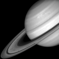
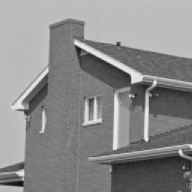
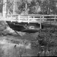
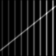
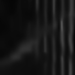
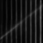
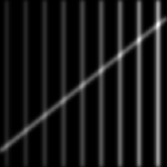
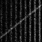
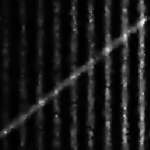
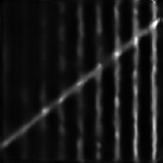
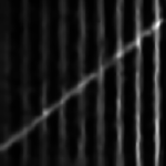
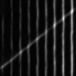
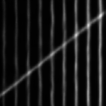
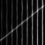
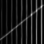
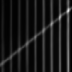
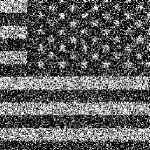
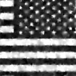
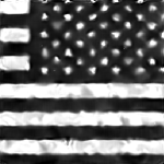
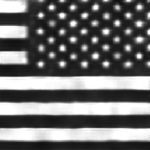
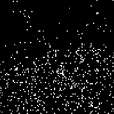
We have first conducted comparisons of our method and several competing algorithms on simulated data. The images we have used in the simulations are presented in Fig. 2. We have considered the same noise level for the Saturn image (cf. Fig. 8) as in Willett06 , where one can find extensive comparisons with a variety of multiscale methods Kolaczyk99 ; Willett_Nowak03 ; Kolaczyk_Nowak04 .

In terms of PSNR, defined in the classical way (for 8-bit images)

$$\operatorname{PSNR}(\widehat{f},f) =10\log_{10}\frac{255^{2}}{\frac{1}{M}{\displaystyle\sum_{i}(\widehat{f}_{i}-f_{i})^{2}}},$$ (20)

our method globally improves upon other state-of-the-art methods such as Poisson-NLM Deledalle_Denis_Tupin10 , SAFIR Boulanger_Kervrann_Bouthemy_Elbau_Sibarita_Salamero10 , and Poisson Multiscale Partitioning (PMP) Willett_Nowak03 for the very low light levels of interest. Moreover, visual artifacts tend to be reduced by our Poisson NLPCA and NLSPCA, with respect to the version using an Anscombe transform and classical PCA (cf. AnscombeNLPCA in Figs. 8 and 6 for instance). See Section 7.4 for more details on the methods used for comparison.

All our results for 2D and 3D images are provided for both the NLPCA and NLSPCA using (except otherwise stated) the parameter values summarized in Table 1. The step-size parameter $\alpha_{t}$ for the NL-SPCA method is chosen via a selection rule initialized with the Barzilai-Borwein choice, as described in Harmany_Marcia_Willett12 .

Parameter	Definition	Value
$N$	patch size	$20\times 20$
$\ell$	approximation rank	4
$K$	clusters	14
$N_{\operatorname{iter}}$	iteration limit	20
$\varepsilon_{{\rm stop}}$	stopping tolerance	$10^{-1}$
$\varepsilon_{\operatorname{cond}}$	conditioning parameter	$10^{-3}$
$\lambda$	$\ell_{1}$ regularization	$70\sqrt{\frac{\log(M_{k})}{n}}$
	(NL-SPCA only)

Table 1: Parameter settings used in the proposed method. Note: $M_{k}$ is the number of patches in the $k$th cluster as determined by the Bregman hard clustering step.

7.2 Simulated 3D data

In this section we have tested a generalization of our algorithm for spectral images. We have thus considered the NASA AVIRIS (Airborne Visible/Infrared Imaging Spectrometer) Moffett Field reflectance data set, and we have kept a $256\times 256\times 128$ sized portion of the total data cube. For the simulation we have used the same noise level as in Krishnamurthy_Raginsky_Willett10 (the number of photons per voxel is 0.0387), so that comparison could be done with the results presented in this paper. Moreover to ease comparison with earlier work, the performance has been measured in terms of mean absolute error (MAE), defined by

$$\operatorname{MAE}(\widehat{f},f)=\frac{\|\widehat{f}-f\|_{1}}{\|f\|_{1}}.$$ (21)

We have performed the clustering on the 2D image obtained by summing the photons on the third (spectral) dimension, and using this clustering for each 3D patch. This approach is particularly well suited for low photons counts since with other approaches the clustering step can be of poor quality. Our approach provides an illustration of the importance of taking into account the correlations across the channels. We have used non-square patches since the spectral image intensity has different levels of homogeneity across the spectral and spatial dimensions. We thus have considered elongated patches with respect to the third dimension. In practice, the patch size used for the results presented is $5\times 5\times 23$, the number of clusters is $K=30$, and the order of approximation is $\ell=2$.

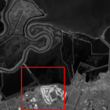
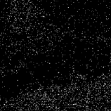
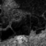
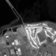
For the noise level considered, our proposed algorithm outperforms the other methods, BM4D Maggioni_Katkovnik_Egiazarian_Foi11 and PMP Krishnamurthy_Raginsky_Willett10 , both visually and in term of MAE (cf. Fig. 7.4.2). Again, these competing methods are described in Section 7.4.

7.3 Real 3D data

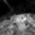
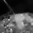
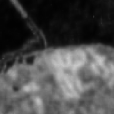
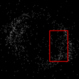
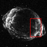
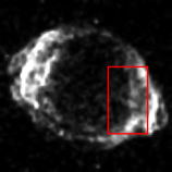
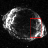
We have also used our method to denoise some real noisy astronomical data. The last image we have considered is based on thermal X-ray emissions of the youngest supernova explosion ever observed. It is the supernova remnant G1.9+0.3 (@ NASA/CXC/SAO) in the Milky Way. The study of such spectral images can provide important information about the nature of elements present in the early stages of supernova. We refer to Borkowski_Reynolds_Green_Hwang_Petre_Krishnamurthy_Willett10 for deeper insights on the implications for astronomical science. This dataset has an average of 0.0137 photons per voxel.

For this image we have also used the 128 first spectral channels, so the data cube is also of size $256\times 256\times 128$. Our method removes some of the spurious artifacts generated by the method proposed in Krishnamurthy_Raginsky_Willett10 and the blurry artifacts in BM4D Maggioni_Katkovnik_Egiazarian_Foi11 .

7.4 Comparison with other methods

7.4.1 Classical PCA with Anscombe transform

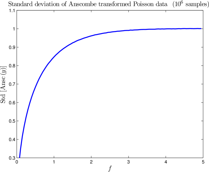
The approximation of the variance provided by the Anscombe transform is reasonably accurate for intensities of three or more (cf. Fig. 3 and also Makitalo_Foi12 Fig. 1-b). In practice this is also the regime where a well-optimized method for Gaussian noise might be applied successfully using this transform and the inverse provided in Makitalo_Foi11 .

Figure 3: Standard deviation approximation of some simulated Poisson data, after performing the Anscombe transform (Ansc). For each true parameter $f$, $10^{6}$ Poisson realizations where drawn and the corresponding standard deviation is reported.

To compare the importance of fully taking advantage of the Poisson model and not using the Anscombe transform, we have derived another algorithm, analogous to our Poisson NLPCA method but using Bregman divergences associated with the natural parameter of a Gaussian random variable instead of Poisson. It corresponds to an implementation similar to the classical power method for computing PCA Collins_Dasgupta_Schapire02 . The function $L$ to be optimized in (10) is simply replaced by the square loss $\tilde{L}$,

$$\tilde{L}(U,V)=\sum_{i=1}^{M}\sum_{j=1}^{N}\left((UV)_{i,j}-Y_{i,j}\right)^{2}\,.$$ (22)

For the Gaussian case, the following update equations are substituted for (13) and (14)

$$U_{t+1,i,:}=U_{t,i,:}-((U_{t}V_{t})_{i,:}-Y_{i,:})V_{t}^{\top}(V_{t}V_{t}^{\top})^{-1}~{},\\$$ (23)

and

$$V_{t+1,:,j}=\\ V_{t,:,j}-(U_{t+1}^{\top}U_{t+1})^{-1}U_{t+1}^{\top}\left((U_{t+1}V_{t})_{:,j}-Y_{:,j}\right)~{}.$$ (24)

An illustration of the improvement due to our direct modeling of Poisson noise instead of a simpler Anscombe (Gaussian) NLPCA approach is shown in our previous work Salmon_Deledalle_Willett_Harmany12 and the below simulation results. The gap is most noticeable at low signal-to-noise ratios, and high-frequency artifacts are more likely to appear when using the Anscombe transform. To invert the Anscombe transform we have considered the function provided by Makitalo_Foi11 , and available at http://www.cs.tut.fi/~foi/invansc/. This slightly improves the usual (closed form) inverse transformation, and in our work it is used for all the methods using the Anscombe transform (referred to as Anscombe-NLPCA in our experiments).

7.4.2 Other methods

We compare our method with other recent algorithms designed for retrieval of Poisson corrupted images. In the case of 2D images we have compared with:

• NLBayes Lebrun_Colom_Buades_Morel12 using Anscombe transform and the refined inverse transform proposed in Makitalo_Foi11 .

• SAFIR Kervrann_Boulanger06 ; Boulanger_Kervrann_Bouthemy_Elbau_Sibarita_Salamero10 , using Anscombe transform and the refined inverse transform proposed in Makitalo_Foi11 .

• Poisson multiscale partitioning (PMP), introduced by Willett and Nowak Willett_Nowak03 ; Willett_Nowak04 using full cycle spinning. We use the haarTIApprox function as available at http://people.ee.duke.edu/~willett.

• BM3D Makitalo_Foi11 using Anscombe transform with a refined inverse transform. The online code is available at http://www.cs.tut.fi/~foi/invansc/ and we used the default parameters provided by the authors. The version with binning and interpolation relies on $3\times 3$ bins and bilinear interpolation.

In the case of spectral images we have compared our proposed method with

• BM4D Maggioni_Katkovnik_Egiazarian_Foi11 using the inverse Anscombe Makitalo_Foi11 already mentioned. We set the patch size to $4\times 4\times 16$, since the patch length has to be dyadic for this algorithm.

• Poisson multiscale partition (PMP for 3D images) Krishnamurthy_Raginsky_Willett10 , adapting the haarTIApprox algorithm to the case of spectral images. As in the reference mentioned, we have considered cycle spinning with 2000 shifts.

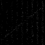
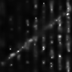
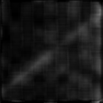
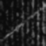
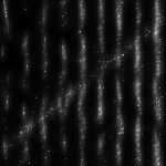
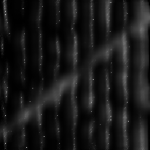
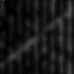
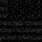
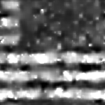
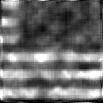
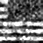
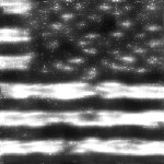
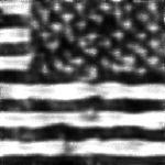
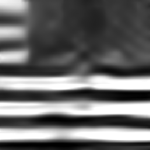
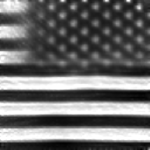
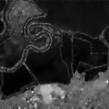
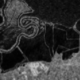
For visual inspection of the qualitative performance of each approach, the results are displayed on Fig. 4-10. Quantitative performance in terms of PSNR are given in Tab. 7.4.2.

(a) Original

(b) Noisy, PSNR=0.31

(c) haarTIApprox, PSNR=18.69

(d) SAFIR, PSNR=17.87

(e) BM3D, PSNR=19.30

(f) AnscombePCA, PSNR=18.08

(g) NLPCA, PSNR=19.26

(h) NLPCAS, PSNR=18.91

(i) BM3Dbin, PSNR=18.99

(j) NLPCASbin, PSNR=23.27

Figure 4: Toy cartoon image (Ridges) corrupted with Poisson noise with Peak = 0.1.

(a) Original

(b) Noisy, PSNR=10.00

(c) haarTIApprox, PSNR=24.44

(d) SAFIR, PSNR=24.92

(e) BM3D, PSNR=26.30

(f) AnscombePCA, PSNR=28.29

(g) NLPCA, PSNR=30.75

(h) NLPCAS, PSNR=30.10

(i) BM3Dbin, PSNR=30.45

(j) NLPCASbin, PSNR=28.32

Figure 5: Toy cartoon image (Ridges) corrupted with Poisson noise with Peak = 1.

(a) Original

(b) Noisy, PSNR=-7.11

(c) haarTIApprox, PSNR=10.97

(d) SAFIR, PSNR=12.04

(e) BM3D, PSNR=12.92

(f) AnscombePCA, PSNR=13.18

(g) NLPCA, PSNR=14.35

(h) NLPCAS, PSNR=14.40

(i) BM3Dbin, PSNR=13.91

(j) NLPCASbin, PSNR=15.99

Figure 6: Toy cartoon image (Flag) corrupted with Poisson noise with Peak = 0.1.

(a) Original

(b) Noisy, PSNR=2.91

(c) haarTIApprox, PSNR=17.82

(d) SAFIR, PSNR=17.91

(e) BM3D, PSNR=18.54

(f) AnscombePCA, PSNR=19.94

(g) NLPCA, PSNR=20.26

(h) NLPCAS, PSNR=20.37

(i) BM3Dbin, PSNR=19.45

(j) NLPCASbin, PSNR=17.12

Figure 7: Toy cartoon image (Flag) corrupted with Poisson noise with Peak = 1.

(a) Original

(b) Noisy, PSNR=-1.70

(c) haarTIApprox, PSNR=21.53

(d) SAFIR, PSNR=21.94

(e) BM3D, PSNR=21.85

(f) AnscombePCA, PSNR=21.84

(g) NLPCA, PSNR=22.96

(h) NLPCAS, PSNR=22.90

(i) BM3Dbin, PSNR=23.17

(j) NLPCASbin, PSNR=22.16

Figure 8: Toy cartoon image (Saturn) corrupted with Poisson noise with Peak = 0.2.

Method	Swoosh	Saturn	Flag	House	Cam	Man	Bridge	Ridges
	Peak $=0.1$
NLBayes	11.08	12.65	7.14	10.94	10.54	11.52	10.58	15.97
haarTIApprox	19.84	19.36	12.72	18.15	17.18	19.10	16.64	18.68
SAFIR	18.88	20.39	12.24	17.45	16.22	18.53	16.55	17.97
BM3D	17.21	19.13	13.12	16.63	15.75	17.24	15.72	19.47
BM3Dbin	21.91	20.82	14.36	18.39	17.11	18.84	16.94	20.33
NLPCA	19.12	20.40	14.45	18.06	16.58	18.48	16.48	21.25
NLSPCA	19.18	20.45	14.50	18.08	16.64	18.49	16.52	20.56
NLSPCAbin	21.56	19.47	15.57	18.68	17.29	18.73	16.90	23.52
	Peak $=0.2$
NLBayes	14.18	14.75	8.20	13.54	12.71	13.89	12.59	16.19
haarTIApprox	21.55	20.91	13.97	19.25	18.37	20.13	17.46	20.46
SAFIR	20.86	21.71	13.65	18.83	17.38	19.88	17.41	18.58
BM3D	20.27	21.20	14.25	18.67	17.44	19.31	17.14	21.10
BM3Dbin	24.14	22.59	16.04	19.93	18.24	20.22	17.66	23.92
NLPCA	21.20	22.29	16.53	19.08	17.80	19.69	17.49	24.10
NLSPCA	21.27	22.34	16.47	19.11	17.77	19.70	17.51	24.41
NLSPCAbin	24.04	20.56	16.65	19.87	17.90	19.61	17.43	25.43
	Peak $=0.5$
NLBayes	19.60	18.28	10.19	17.01	15.68	16.90	15.11	16.77
haarTIApprox	23.59	23.27	16.25	20.65	19.59	21.30	18.32	23.07
SAFIR	22.70	24.23	16.20	20.37	18.84	21.25	18.42	20.90
BM3D	23.53	24.09	15.94	20.50	18.86	21.03	18.37	23.33
BM3Dbin	26.20	25.64	18.53	21.70	19.58	21.60	18.75	27.99
NLPCA	24.50	25.38	18.93	20.78	19.36	21.13	18.47	28.06
NLSPCA	24.44	25.06	18.92	20.76	19.23	21.12	18.46	28.03
NLSPCAbin	26.36	20.67	17.09	20.97	18.39	20.28	18.16	26.81
	Peak $=1$
NLBayes	23.58	21.66	14.00	19.27	17.99	19.48	16.85	18.35
haarTIApprox	25.12	25.06	17.79	21.97	20.64	22.25	19.08	24.52
SAFIR	23.37	25.14	17.91	21.46	20.01	22.08	19.12	24.67
BM3D	26.21	25.88	18.45	22.26	20.45	22.27	19.39	25.76
BM3Dbin	27.95	27.24	19.49	23.26	20.61	22.53	19.47	29.91
NLPCA	26.99	27.08	20.23	22.07	20.31	21.96	19.01	30.17
NLSPCA	27.02	27.04	20.37	22.10	20.28	21.88	19.00	30.04
NLSPCAbin	27.21	21.10	17.03	21.21	18.45	20.37	18.36	26.96
	Peak $=2$
NLBayes	27.50	24.66	17.13	21.10	19.67	21.34	18.22	21.04
haarTIApprox	27.01	26.43	19.33	23.37	21.72	23.18	19.90	26.53
SAFIR	23.78	26.02	19.25	22.33	21.30	22.74	19.99	28.29
BM3D	28.63	27.70	20.66	24.25	22.19	23.54	20.44	29.75
BM3Dbin	29.70	28.68	20.01	24.52	21.42	23.43	20.17	32.24
NLPCA	29.41	28.02	20.64	23.44	20.75	22.78	19.37	32.25
NLSPCA	29.53	28.11	20.75	23.75	20.76	22.86	19.45	32.35
NLSPCAbin	27.62	21.13	17.02	21.42	18.33	20.34	18.34	29.31
	Peak $=4$
NLBayes	31.17	26.73	22.64	23.61	22.32	23.02	19.60	24.04
haarTIApprox	28.55	28.13	21.16	24.88	22.93	24.23	20.83	28.56
SAFIR	25.40	27.40	20.71	23.76	22.73	23.85	20.88	30.52
BM3D	30.36	29.30	22.91	26.08	23.93	24.79	21.50	32.50
BM3Dbin	31.15	30.07	20.57	25.64	22.00	24.28	20.84	33.52
NLPCA	31.08	29.07	20.96	24.49	20.96	23.18	19.73	33.73
NLSPCA	31.46	29.51	21.15	24.89	21.08	23.41	20.15	33.69
NLSPCAbin	27.65	21.45	16.00	21.47	18.44	20.35	18.35	29.13

Table 2: Experiments on simulated data (average over five noise realizations). Flag and Saturn images are displayed in Figs. 8, 6 and 7, and the others are given in Salmon_Willett_AriasCastro12 and in Zhang_Fadili_Starck08 .

(a) Original, channel 68

(b) Noisy data

(c) BM4D, $4\times 4\times 16$ MAE=0.2426

(d) Multiscale partition, MAE=0.1937

(e) NLSPCA, $5\times 5\times 23$, MAE=0.1893

(f) Original, channel 68

(g) Noisy data

(h) BM4D, $4\times 4\times 16$, MAE=0.2426

(i) Multiscale partition, MAE=0.1937,

(j) NLSPCA, $5\times 5\times 23$, MAE=0.1893

Figure 9: Original and close-up of the red square from spectral band 68 of the Moffett Field. The same methods are considered, and are displayed in the same order: original, noisy (with 0.0387 photons per voxels), BM4D Maggioni_Katkovnik_Egiazarian_Foi11 (with inverse Anscombe as in Makitalo_Foi11 ), multiscale partitioning method Krishnamurthy_Raginsky_Willett10 , and our proposed method with patches of size $5\times 5\times 23$.

(a) Noisy (channel 101)

(b) Average over channels

(c) BM4D, $4\times 4\times 16$

(d) Multiscale partition

(e) NLSPCA, $5\times 5\times 23$

Figure 10: Spectral image of the supernova remnant G1.9+0.3. We display the spectral band 101 of the noisy observation (with 0.0137 photons per voxels), and this denoised channel with BM4D Maggioni_Katkovnik_Egiazarian_Foi11 (with inverse Anscombe as in Makitalo_Foi11 ), the multiscale partitioning method Krishnamurthy_Raginsky_Willett10 , and our proposed method NLSPCA with patches of size $5\times 5\times 23$. Note how the highlighted detail shows structure in the average over channels, which appears to be accurately reconstructed by our method.

8 Conclusion and future work

Inspired by the methodology of Deledalle_Salmon_Dalalyan11 we have adapted a generalization of the PCA Collins_Dasgupta_Schapire02 ; Roy_Gordon_Thrun05 for denoising images damaged by Poisson noise. In general, our method finds a good rank-$\ell$ approximation to each cluster of patches. While this can be done either in the original pixel space or in a logarithmic “natural parameter” space, we choose the logarithmic scale to avoid issues with nonnegativity, facilitating fast algorithms. One might ask whether working on a logarithmic scale impacts the accuracy of this rank-$\ell$ approximation. Comparing against several state-of-the-art approaches, we see that because our approach often works as well or better than these alternatives, the exponential formulation of PCA does not lose significant approximation power or else it would manifest itself in these results.

Possible improvements include adapting the number of dictionary elements used with respect to the noise level, and proving a theoretical convergence guarantees for the algorithm. The nonconvexity of the objective may only allow convergence to local minima. An open question is whether these local minima have interesting properties. Reducing the computational complexity of NLPCA is a final remaining challenge.

Acknowledgments

Joseph Salmon, Zachary Harmany, and Rebecca Willett gratefully acknowledge support from DARPA grant no. FA8650-11-1-7150, AFOSR award no. FA9550-10-1-0390, and NSF award no. CCF-06-43947. The authors would also like to thank J. Boulanger and C. Kervrann for providing their SAFIR algorithm, Steven Reynolds for providing the spectral images from the supernova remnant G1.9+0.3, and an anonymous reviewer for proposing the improvement using the binning step.

Appendix

Appendix A Biconvexity of loss function

Lemma 1

The function $L$ is biconvex with respect to $(U,V)$ but not jointly convex.

Proof

The biconvexity argument is straightforward; the partial functions $U\mapsto L(U,V)$ with a fixed $V$ and $V\mapsto L(U,V)$ with a fixed $U$ are both convex. The fact that the problem is non-jointly convex can be seen when $U$ and $V$ are in $\mathbb{R}$ (i.e., $\ell=m=n=1$), since the Hessian in this case is

$$H_{L}(U,V)=\begin{pmatrix}V^{2}e^{UV}&UVe^{UV}+e^{UV}-Y\\ UVe^{UV}+e^{UV}-Y&U^{2}e^{UV}\end{pmatrix}.$$

Thus at the origin one has $H_{L}(0,0)=\begin{pmatrix}0&1\\ 1&0\end{pmatrix}$, which has a negative eigenvalue, $-1$.

Appendix B Gradient calculations

We provide below the gradient computation used in Eq. (13) and Eq. (14):

$$\nabla_{U}L(U,V) =(\exp(UV)-Y)V^{\top}\,,$$

$$\nabla_{V}L(U,V) =U^{\top}(\exp(UV)-Y)\,.$$

Using the component-wise representation this is equivalent to

$$\frac{\partial L(U,V)}{\partial U_{a,b}} =\displaystyle\sum_{j=1}^{N}\exp(UV)_{a,j}V_{b,j}-Y_{a,j}V_{b,j}\,,$$

$$\frac{\partial L(U,V)}{\partial V_{a,b}} =\displaystyle\sum_{i=1}^{M}U_{i,a}\exp(UV)_{i,b}-U_{i,a}Y_{i,b}\,.$$

Appendix C Hessian calculations

The approach proposed by Gordon03 ; Roy_Gordon_Thrun05 consists in using an iterative algorithm which sequentially updates the $j$th column of $V$ and the $i$th row of $U$. The only problem with this method is numerical: one needs to invert possibly ill conditioned matrices at each step of the loop.

The Hessian matrices of our problems, with respect to $U$ and $V$ respectively are given by

$$\frac{\partial^{2}L(U,V)}{\partial U_{a,b}\partial U_{c,d}}=\left\{\begin{array}[]{ll}\displaystyle\sum_{j=1}^{N}\exp(UV)_{a,j}V^{2}_{b,j},&\mbox{if }(a,b)=(c,d),\\ 0&\mbox{otherwise,}\end{array}\right.$$

and

$$\frac{\partial^{2}L(U,V)}{\partial V_{a,b}\partial V_{c,d}}=\left\{\begin{array}[]{ll}\displaystyle\sum_{i=1}^{M}U^{2}_{i,a}\exp(UV)_{i,b},&\mbox{if }(a,b)=(c,d),\\ 0&\mbox{otherwise.}\end{array}\right.$$

Notice that both Hessian matrices are diagonal. So applying the inverse of the Hessian simply consists in inverting the diagonal coefficients.

Appendix D The Newton step

In the following we need to introduce the function $\operatorname{Vect}_{C}$ that transforms a matrix into one single column (concatenates the columns), and the function $\operatorname{Vect}_{R}$ that transforms a matrix into a single row (concatenates the rows). This means that

$$\operatorname{Vect}_{C}:\, \mathbb{R}^{M\times\ell} \longrightarrow ~{}\mathbb{R}^{M\ell\times 1}\,,$$

$$U=(U_{1,:},\cdots,U_{\ell,:}) \longmapsto ~{}(U_{1,:}^{\top},\cdots,U_{\ell,:}^{\top})^{\top},$$

and

$$\operatorname{Vect}_{R}:\, \mathbb{R}^{\ell\times N} \longrightarrow ~{}\mathbb{R}^{1\times\ell N}\,,$$

$$V=(V_{:,1}^{\top},\cdots,V_{:,\ell}^{\top})^{\top} \longmapsto ~{}(V_{:,1},\cdots,V_{:,\ell}).$$

Now using the previously introduced notations, the updating steps for $U$ and $V$ can be written

$$\operatorname{Vect}_{C}(U_{t+1}) =\operatorname{Vect}_{C}(U_{t})-H_{U_{t}}^{-1}\operatorname{Vect}_{C}\big{(}\nabla_{U}L(U_{t},V_{t})\big{)}\,,$$ (25)

$$\operatorname{Vect}_{R}(V_{t+1}) =\operatorname{Vect}_{R}(V_{t})-\operatorname{Vect}_{R}\big{(}\nabla_{V}L(U_{t},V_{t})\big{)}H_{V_{t}}^{-1}\,.$$ (26)

We give the order used to concatenate the coefficients for the Hessian matrix with respect to $U$, $H_{U}$: $(a,b)=(1,1),\cdots,(M,1),(1,2),\cdots(M,2),\cdots(1,\ell),\cdots,(M,\ell)$.

We concatenate the column of $U$ in this order.

It is easy to give the updating rules for the $k$th column of $U$, one only needs to multiply the first Equation of (25) from the left by the $M\times M\ell$ matrix

$$F_{k,M,\ell,}=\begin{pmatrix}0_{M,M},&\cdots,&I_{M,M},&\cdots,&0_{M,M}\end{pmatrix}$$ (27)

where the identity block matrix is in the $k$th position. This leads to the following updating rule

$${U_{t+1,\cdot,k}=U_{t,:,k}-D_{k}^{-1}(\exp(U_{t}V_{t})-Y)V_{t,k,:}^{\top}}~{},$$ (28)

where $D_{k}$ is a diagonal matrix of size $M\times M$:

$$\begin{split}D_{k}=\operatorname{diag}\Big{(}\displaystyle\sum_{j=1}^{n}\exp(U_{t}V_{t})_{1,j}&V^{2}_{t,k,j},\cdots,\\ &\displaystyle\sum_{j=1}^{n}\exp(U_{t}V_{t})_{M,j}V^{2}_{t,k,j}\Big{)}.\end{split}$$

This leads easily to (13).

By the symmetry of the problem in $U$ and $V$, one has the following equivalent updating rule for $V$:

$${V_{t+1,k,:}=V_{t,k,:}-U_{t,:,k}^{\top}(\exp(U_{t}V_{t})-Y)E_{k,M}^{-1}}~{},$$ (29)

where $E_{k}$ is a diagonal matrix of size $N\times N$:

$$\begin{split}E_{k}=\operatorname{diag}\Big{(}\displaystyle\sum_{i=1}^{M}\exp(U_{t}V_{t})_{i,1}&U^{2}_{t,i,k},\cdots,\\ &\displaystyle\sum_{j=1}^{n}\exp(U_{t}V_{t})_{i,n}U^{2}_{t,i,k}\Big{)}.\end{split}$$

References

- [1] M. Aharon, M. Elad, and A. Bruckstein. K-SVD: An algorithm for designing overcomplete dictionaries for sparse representation. IEEE Trans. Signal Process., 54(11):4311–4322, 2006.
- [2] F. J. Anscombe. The transformation of Poisson, binomial and negative-binomial data. Biometrika, 35:246–254, 1948.
- [3] A. Banerjee, S. Merugu, I.S. Dhillon, and J. Ghosh. Clustering with Bregman divergences. J. Mach. Learn. Res., 6:1705–1749, 2005.
- [4] K. J. Borkowski, S. P. Reynolds, D. A. Green, U. Hwang, R. Petre, K. Krishnamurthy, and R. Willett. Radioactive Scandium in the youngest galactic supernova remnant G1. 9+ 0.3. The Astrophysical Journal Letters, 724:L161, 2010.
- [5] J. Boulanger, C. Kervrann, P. Bouthemy, P. Elbau, J-B. Sibarita, and J. Salamero. Patch-based nonlocal functional for denoising fluorescence microscopy image sequences. IEEE Trans. Med. Imag., 29(2):442–454, 2010.
- [6] S. Boyd, N. Parikh, E. Chu, B. Peleato, and J. Eckstein. Distributed optimization and statistical learning via the alternating direction method of multipliers. Foundations and Trends in Machine Learning, 3(1):1–122, 2011.
- [7] L. M. Bregman. The relaxation method of finding the common point of convex sets and its application to the solution of problems in convex programming. Comput. Math. Math. Phys., 7(3):200–217, 1967.
- [8] A. Buades, B. Coll, and J-M. Morel. A review of image denoising algorithms, with a new one. Multiscale Model. Simul., 4(2):490–530, 2005.
- [9] P. Chatterjee and P. Milanfar. Patch-based near-optimal image denoising. In ICIP, 2011.
- [10] M. Collins, S. Dasgupta, and R. E. Schapire. A generalization of principal components analysis to the exponential family. In NIPS, pages 617–624, 2002.
- [11] K. Dabov, A. Foi, V. Katkovnik, and K. O. Egiazarian. Image denoising by sparse 3-D transform-domain collaborative filtering. IEEE Trans. Image Process., 16(8):2080–2095, 2007.
- [12] K. Dabov, A. Foi, V. Katkovnik, and K. O. Egiazarian. BM3D image denoising with shape-adaptive principal component analysis. In Proc. Workshop on Signal Processing with Adaptive Sparse Structured Representations (SPARS’09), 2009.
- [13] A. Danielyan, A. Foi, V. Katkovnik, and K. Egiazarian. Denoising of multispectral images via nonlocal groupwise spectrum-PCA. In CGIV2010/MCS’10, pages 261–266, 2010.
- [14] C-A. Deledalle, L. Denis, and F. Tupin. Poisson NL means: Unsupervised non local means for Poisson noise. In ICIP, pages 801–804, 2010.
- [15] C-A. Deledalle, J. Salmon, and A. S. Dalalyan. Image denoising with patch based PCA: Local versus global. In BMVC, 2011.
- [16] M. A. T. Figueiredo and J. M. Bioucas-Dias. Restoration of poissonian images using alternating direction optimization. IEEE Trans. Signal Process., 19(12):3133–3145, 2010.
- [17] M. Fisz. The limiting distribution of a function of two independent random variables and its statistical application. Colloquium Mathematicum, 3:138–146, 1955.
- [18] P. Fryźlewicz and G. P. Nason. Poisson intensity estimation using wavelets and the Fisz transformation. Technical report, Department of Mathematics, University of Bristol, United Kingdom, 2001.
- [19] G. J. Gordon. Generalized linear models. In NIPS, pages 593–600, 2003.
- [20] Z. Harmany, R. Marcia, and R. Willett. This is SPIRAL-TAP: Sparse Poisson Intensity Reconstruction ALgorithms – Theory and Practice. IEEE Trans. Image Process., 21(3):1084–1096, 2012.
- [21] V. Katkovnik, A. Foi, K. O. Egiazarian, and J. T. Astola. From local kernel to nonlocal multiple-model image denoising. Int. J. Comput. Vision, 86(1):1–32, 2010.
- [22] C. Kervrann and J. Boulanger. Optimal spatial adaptation for patch-based image denoising. IEEE Trans. Image Process., 15(10):2866–2878, 2006.
- [23] E. D. Kolaczyk. Wavelet shrinkage estimation of certain Poisson intensity signals using corrected thresholds. Statist. Sinica, 9(1):119–135, 1999.
- [24] E. D. Kolaczyk and R. D. Nowak. Multiscale likelihood analysis and complexity penalized estimation. Ann. Statist., 32(2):500–527, 2004.
- [25] K. Krishnamurthy, M. Raginsky, and R. Willett. Multiscale photon-limited spectral image reconstruction. SIAM J. Imaging Sci., 3(3):619–645, 2010.
- [26] M. Lebrun, M. Colom, A. Buades, and J-M. Morel. Secrets of image denoising cuisine. Acta Numerica, 21(1):475–576, 2012.
- [27] H. Lee, A. Battle, R. Raina, and A. Y. Ng. Efficient sparse coding algorithms. In NIPS, pages 801–808, 2007.
- [28] M. Maggioni, V. Katkovnik, K. Egiazarian, and A. Foi. A nonlocal transform-domain filter for volumetric data denoising and reconstruction. submitted, 2011.
- [29] J. Mairal, F. Bach, J. Ponce, and G. Sapiro. Online learning for matrix factorization and sparse coding. J. Mach. Learn. Res., pages 19–60, 2010.
- [30] J. Mairal, F. Bach, J. Ponce, G. Sapiro, and A. Zisserman. Non-local sparse models for image restoration. In ICCV, pages 2272–2279, 2009.
- [31] M. Mäkitalo and A. Foi. Optimal inversion of the Anscombe transformation in low-count Poisson image denoising. IEEE Trans. Image Process., 20(1):99–109, 2011.
- [32] M. Mäkitalo and A. Foi. Optimal inversion of the generalized anscombe transformation for poisson-gaussian noise. submitted, 2012.
- [33] D. D. Muresan and T. W. Parks. Adaptive principal components and image denoising. In ICIP, pages 101–104, 2003.
- [34] F. Nielsen and V. Garcia. Statistical exponential families: A digest with flash cards. Arxiv preprint arXiv:0911.4863, 2009.
- [35] N. Roy, G. J. Gordon, and S. Thrun. Finding approximate POMDP solutions through belief compression. J. Artif. Intell. Res., 23(1):1–40, 2005.
- [36] J. Salmon, C-A. Deledalle, R. Willett, and Z. Harmany. Poisson noise reduction with non-local PCA. In ICASSP, 2012.
- [37] J. Salmon and Y. Strozecki. Patch reprojections for Non Local methods. Signal Processing, 92(2):447–489, 2012.
- [38] J. Salmon, R. Willett, and E. Arias-Castro. A two-stage denoising filter: the preprocessed Yaroslavsky filter. In SSP, 2012.
- [39] A. P. Singh and G. J. Gordon. Relational learning via collective matrix factorization. In Proceeding of the 14th ACM SIGKDD international conference on Knowledge discovery and data mining, pages 650–658. ACM, 2008.
- [40] A. P. Singh and G. J. Gordon. A unified view of matrix factorization models. Machine Learning and Knowledge Discovery in Databases, pages 358–373, 2008.
- [41] R. Willett. Multiscale Analysis of Photon-Limited Astronomical Images. In Statistical Challenges in Modern Astronomy (SCMA) IV, 2006.
- [42] R. Willett and R. D. Nowak. Platelets: A multiscale approach for recovering edges and surfaces in photon-limited medical imaging. IEEE Trans. Med. Imag., 22(3):332–350, 2003.
- [43] R. Willett and R. D. Nowak. Fast multiresolution photon-limited image reconstruction. In Proc. IEEE Int. Sym. Biomedical Imaging — ISBI ’04, 2004.
- [44] S. J. Wright, R. D. Nowak, and M. A. T. Figueiredo. Sparse reconstruction by separable approximation. IEEE Trans. Signal Process., 57(7):2479–2493, 2009.
- [45] W. Yin, S. Osher, D. Goldfarb, and J. Darbon. Bregman iterative algorithms for l1-minimization with applications to compressed sensing. SIAM J. Imaging Sci., 1(1):143–168, 2008.
- [46] B. Zhang, J. Fadili, and J-L. Starck. Wavelets, ridgelets, and curvelets for Poisson noise removal. IEEE Trans. Image Process., 17(7):1093–1108, 2008.
- [47] L. Zhang, W. Dong, D. Zhang, and G. Shi. Two-stage image denoising by principal component analysis with local pixel grouping. Pattern Recogn., 43(4):1531–1549, 2010.
- [48] H. Zou, T. Hastie, and R. Tibshirani. Sparse principal component analysis. J. Comput. Graph. Statist., 15(2):265–286, 2006.