A New Class of Parametrization for Dark Energy without Divergence
Abstract
In this paper, we propose a new class of parametrization of the equation of state of dark energy. In contrast with the famous CPL parametrization, these new parametrization of the equation of state does not divergent during the evolution of the Universe even in the future. Also, we perform a observational constraint on two simplest dark energy models belonging to this new class of parametrization, by using the Markov Chain Monte Carlo (MCMC) method and the combined latest observational data from the type Ia supernova compilations including Union2(557), cosmic microwave background, and baryon acoustic oscillation.
I Introduction
The cosmic acceleration has been discovered since 1998 Riess:1998cb ; Perlmutter:1998np , but we are still in the dark about the nature of this mystery. The cosmological constant proposed by Einstein to build a static Universe solution is the simplest dark energy model to explain the acceleration, but it suffers from the fine-tuning and coincidence problems. On the other side, current observations do not exclude definitely the time dependent evolution of dark energy, then many alternative dark energy models were proposed in the literatures, for a recent review, see Li:2011sd ; Bamba:2012cp .
The evolution of dark energy is determined by its equation of state (EoS), which can be obtained in a particular model or constructed directly from observational data. In the later case, we usually make some assumptions on the form of the EoS as a parametrization for the dark energy model, then extract the information from observations. A most wildly used parametrization is called the Chevallier-Polarski-Linder (CPL) model Chevallier:2000qy ; Linder:2002et with the form of EoS as
| (1) |
with redshift . Here, is the present value of the EoS and is the derivative with respect to the scale factor. Comparing with the linear form , the CPL parametrization is well behaved and bounded at high redshifts. This is the direct motivation of proposing such a form (1). However, the CPL form also suffers from the divergence problem when approaches , which corresponds to future evolution of the EoS. This is undoubtedly a nonphysical feature, and thus it prevents the CPL parametrization from genuinely covering the scalar field models as well as other theoretical models. Recently, a logarithm form and an oscillating form are proposed in Ref. Ma:2011nc ; Li:2011dr ; Li:2012vn to overcome the shortcoming of the CPL model.
To extend parametrization of dark energy to redshifts , we suggest two new models
| (2) |
and
| (3) |
which are free of divergence in the whole range of the redshift . Clearly, Model I reduce to the linear form when as the CPL form, while Model II will be not. Actually, one can even generalize the form to a more general case while keeps the advantage of divergence-free, as long as some conditions are satisfied. We will make some discussions about it in the conclusion section, and one shall see that the forms (2) and (3) are the most simplest ones of this class of parametrization.
We perform a global data fitting analysis on these two divergence-free parametrization of dark energy models and constrain the parameters from the current observational data, including the full CMB power spectrum from seven-year WMAP data (WMAP7) Komatsu:2010fb , the baryon acoustic oscillations (BAO) data from SDSS DR7 Percival:2009xn and Union2 SNIa with samples Amanullah:2010vv . When doing the analysis, we also take the perturbation of dark energy into account, because the perturbation plays a important role when one confronts the dynamical dark energy models with the current observations Zhao:2005vj ; Li:2010hm ; Hwang:2009zj ; Feng:2009ag . For instance, when the dark energy dominates the Universe at later time in a spatial flat model, the gravitational potential due to the perturbation of dark energy becomes time-dependent, thus there will be a significant imprint on the large-scale CMB power spectra by the integrated Sachs-Wolfe (ISW) effect Sachs:1967er ; Bean:2003fb ; Schaefer:2008qs ; Wang:2010zzj ; Wang:2010cg ; Sapone:2009mb . We also make some analysis on this effect in this paper. We added two new parameters and modified the public available CosmoMC package Lewis:2002ah to satisfy these two models. During the calculation, we run independent chains for each case, and we make sure the convergence of the chains by typically getting to be less than , see Ref. Lewis:2002ah ; Feng:2012gr ; Ao:2011kc ; Feng:2009zf ; Liu:2008vy and the readme file on the website of CosmoMC.
This paper is organized as follows: In Sec.II, we will study the background and perturbation evolutions for both models. In Sec.III, we perform a global fitting to the current observational data by using the Markov Chain Monte Carlo (MCMC) method. Some analysis on the ISW effect of there two models are given in Sec.IV. In the last section, we will give some conclusions and make some discussions on how to generalize these models without losing the advantage of divergence-free.
II Background and Perturbation Evolution
As we mentioned before, the new parametrizations of dark energy (2) and (3) are free of divergence in the whole range of the redshift , especially when . For clearness, we list the limiting values of when in Tab.1 for the CPL model, Model I and Model II.
| Model | ||||
|---|---|---|---|---|
| CPL | ||||
| Model I | ||||
| Model II |
At low shifts, the Model I form will reduce to the linear form as the CPL model, while Model II will reduce to the quadratic form, i.e. , and both of them are free of divergence. From the continuity equation of the dark energy with EoS (2) and (3), one can obtain the its energy density, and then the Friedmann equation would be
| (4) |
for a spacial flat Universe. Here we have defined and . The functions are given by
| (5) |
where and correspond to Model I and II, respectively.
As we known, for dynamical dark energy models, namely, the EoS of dark energy is not constantly equal to , it is crucial to include dark energy perturbations Zhao:2005vj ; Li:2010hm ; Hwang:2009zj ; Feng:2009ag . Working in the conformal Newtonian gauge with the perturbed metric as the following
| (6) |
one can obtain the perturbed equations of dark energy as Ma:1995ey ; Bardeen:1980kt ; Kodama:1985bj
| (7) | |||||
| (8) |
where prime denotes the derivatives with respect to conformal time , is the conformal Hubble parameter. Here and are the density and velocity perturbations respectively. The square sound speed is defined as . It is clear that for the quintessence-like (or phantom-like) models with (or ), the perturbation equations (7) and (8) are well-defined. In other words, as long as the EoS does not cross the cosmological boundary, the perturbation equations will not divergence. However, when the cross happens in the dark energy models such as CPL, Model I and II, one should take care when . This is so-called the divergence problem for perturbations of dark energy. A very useful practical solution to this problem is to introduce a small positive constant , then the whole range of the allowed values of EoS is divided into three parts: , and , see Ref. Zhao:2005vj . For the first two regions, the perturbation equations are well-defined without divergence. To avoid the divergence in the last region, we take the approach that match the perturbations in this region to the first two regions at the boundary and set in this region. In our numerical calculations, we limit the range to be , suggested in Ref. Wang:2011km .
III Global Fitting Procedure and Results
In this section, we will use the Markov Chain Monte Carlo (MCMC) method to make a global fitting on the cosmological parameters in Model I and II. We have modified the public available CosmoMC package Lewis:2002ah to satisfy Model I and II, in which we have added two new parameters and and the perturbation equations for dark energy. Our most general parameter space vector is
| (9) |
where and are the physical baryon and cold dark matter densities, is the ratio (multiplied by ) of the sound horizon to the angular diameter distance at decoupling, is the optical depth to re-ionization, and are the parameters of dark energy EoS given by Eqs.(2) and (3), is the scalar spectral index and is defined as the amplitude of the initial power spectrum. The pivot scale of the initial scalar power spectrum we used here is Mpc-1 and we have assumed purely adiabatic initial conditions. In this paper, we will use the WMAP seven-year data Komatsu:2010fb , the BAO data Percival:2009xn and also the current supernova ”Union2” data with simples Amanullah:2010vv . All the calculations are performed on the Astrophysical Beowulf Cluster (AstroBC), which is a parallel computing network system designed, set up and tested by ourselves, and it is much fast and stable than a single personal computer.
In order to determine the best value of parameters (with error at least ) in Model I and II, we will use the maximum likelihood method and take the total likelihood function as the products of these separate likelihood functions of each data set, thus we get
| (10) |
Then, one can get the best fitting values of parameters by minimizing .
Our global fitting results are presented in Tab.2, in which we list the best fit values with errors for each parameter in the parameter space vector (9), as well as the constraint for the age of the Universe. For comparison, we also present the fitting results without dark energy perturbations in Tab.2, and we find that the results with perturbations show a better fit to that without perturbations by comparing the minimal values of . In our analysis, we have fixed the sound speed of dark energy in the rest frame , which related to in a general frame as Bean:2003fb ; Kodama:1985bj
| (11) |
To derive the above relation, we have used the useful relation between the gauge invariant, rest frame density perturbation and the density and velocity perturbations in a general frame, and
| (12) |
and the definition of the adiabatic sound speed
| (13) |
see Ref.Bean:2003fb ; Kodama:1985bj . Since it has been shown that the constraints on the dark energy sound speed in the rest frame in dynamical dark energy models are still not accurate enough Xia:2007km , then one can treats the dark energy model as a effective scalar-field model and sets to be unit Li:2011dr . The results would not be affected by this treatment if is considered as a free parameter. In this paper, we have taken the full CMB temperature and polarization power spectra instead of just taking the WMAP distance prior, including and , which encoding the background distance information and can be used to investigate dark energy models with greatly simplified numerical calculations. However, it was found that this distance prior is somewhat cosmological model dependent, thus, one would loss some CMB information by using it to fit the parameters Komatsu:2010fb . For instance, as we known, if there was a time-dependent gravitational potential at later times, it will contribute to the ISW effect. Therefore, our results would be more reliable than that obtained by using just the distance prior.
| Model Parameter | Model I | Model II | ||
| w/. perturb. | w/o. perturb. | w/. perturb. | w/o. perturb. | |
| Data | CMB BAO SN | |||
| Age/Gyr | ||||
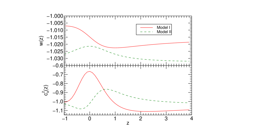
From Tab.2, one can see that in both models, the best-fit values of the scalar spectral index are smaller than . That is to say, the scalar spectrum is ”red” tiled. The difference between Model I and II is shown in Fig.1, in which we have plotted the evolution of the EoS and the adiabatic square sound speed for both models with their best-fit values of and . From Fig.1, we find that the best-fit dark energy model is a phantom model, whose is always smaller than , and the evolution of is quite different between these two models. However, the difference of the present values of is smaller than one percent. These results imply that though the dynamical dark energy models are mildly favored, the current data cannot distinguish them effectively.

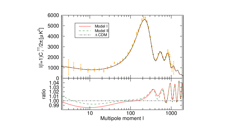
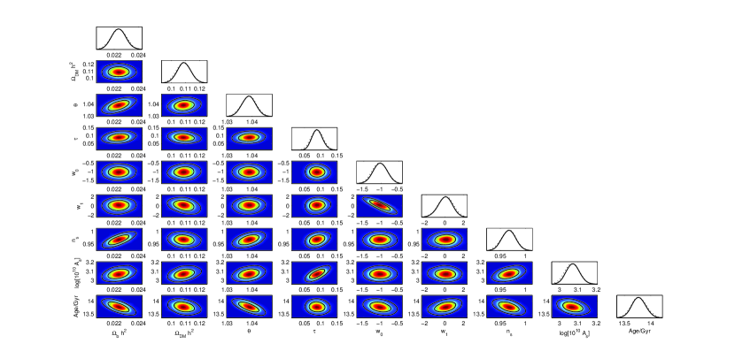
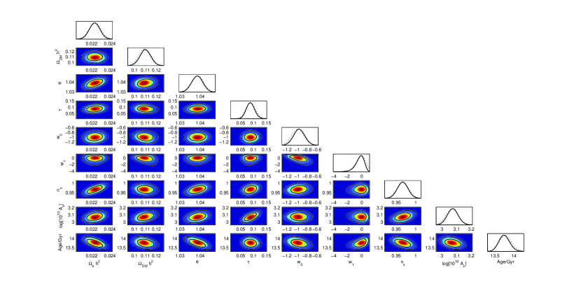
In Fig. 2, we show the CMB temperature power spectrum for Model I and II with their best-fit parameters listed in Tab. 2. The spectrum for CDM is also plotted for comparison. We find that the most significant discrepancies between Model I, II and CDM come from the low s, or large angular scales (). The contribution to the secondary CMB anisotropy is mainly contributed from the late ISW effect, see the discuss in next section. Both cures of Model I and II tend to be plat on large scales. In the Fig.3 and Fig.4, we also show the one dimensional probability distribution of each parameters and also the two dimensional contour plots between each other in the Model I and II from combination of WMAP, SN and BAO.


IV The ISW Effect
The ISW effect is due to the existence of time-dependent gravitational potentials along the line of sight from the epoch of last scattering up to now Sachs:1967er ; Hu:1994jd ; Hu:1995sv . There is a net change in the energy of a CMB photon as it passes through these evolving gravitational potential wells, and the sum of these contributions is called the ISW effect. The ISW contribution to the CMB power in the th multipole is given by
| (14) |
where is the multipole decomposition of the fractional fluctuation due to the ISW effect
| (15) |
Here, and denote the present and the last scattering conformal times respectively, and are the spherical Bessel functions. As we known, the perturbation equation of is given by
| (16) |
where . The adiabatic square sound speed in a dark energy dominated Universe is given by Eq. (13), and one can rewritten in terms of redshift
| (17) |
where takes the form of (2) and (3). And thus, we obtain
| (18) |
and
| (19) |
The evolution of is shown in Fig. 1 in Model I and II.
It is usual to divide the ISW effect into early and late parts. The early ISW effect corresponds to the variation in the perturbation potentials which occurs in the time interval between matter-radiation equality and recombination, while the late ISW effect corresponds to the variations caused by the presence of dark energy. The expansion time scale at dark energy domination sets a critical wavelength corresponding to . Thus, for adiabatic perturbations, the late ISW effect in Eq. (15) during the dark energy epoch for a given mode can be approximated by Hu:1994jd ; Hu:1995sv
| (20) |
where is the conformal time when a given -mode contributes maximally to the angle that this scale subtends on the sky, which obtained at the peak of the Bessel function . Here the integral is given by
| (21) |
Substituting the results above into Eq. (14), we obtain the momenta of the late ISW effect
| (22) |
Therefore, one can at least numerically obtain the solution of from Eq. (16) and then get s. From Eq. (22), one can see that the main contribution of the late ISW effect mainly comes from the low momenta , see Fig. 2.
V Discussion and Conclusion
In this paper, we have proposed two new parametrizations for the EoS of dark energy, see Eqs.(2) and (3). Actually, these two models belong to the following general case
| (23) |
where Model I corresponds to and Model II corresponds to . From the above equation, one can see that as long as is a non-zero integer, would be not divergent when , and the limiting value is . Furthermore, if , the EoS would be also not divergent when the redshift goes to infinite. The limiting values for when and are and . In general, one can not get an analytic result for the function in the background equation (4), and usually it is given by the following integration
| (24) |
It is interesting that in Model I, the EoS could be rewritten as
| (25) |
from which one can see that when the redshifts are large (), while when the redshifts are small (), in other words, the EoS of Model I has the symmetry of .
In conclusion, we have performed a global fit study on two parametrization models for dark energy, named Model I and II. In contrast to the famous CPL parametrization, in which is divergent when , Model I and II overcome this shortcoming and are divergence-free in the whole range of the redshifts . We have not only obtained the best-fit values with and regions for both of Model I and II with and without dark energy perturbations, but also found that the differences of CMB temperature power spectrum on large angular scales are significant between Model I, II and CDM model. There also exists a flat plateau on the large scales in both models. In view of this difference, on which the ISW effect plays an important role. The effects on the parametrizations of Model I and II made by the ISW data from the correlations of CMB and large scale structure will be studied in our further works. And the class of this parametrization (23) is also worth investigating in future.
Acknowledgements.
This work is supported by National Science Foundation of China grant Nos. 11105091 and 11047138, National Education Foundation of China grant No. 2009312711004, Shanghai Natural Science Foundation, China grant No. 10ZR1422000, and Shanghai Special Education Foundation, No. ssd10004.References
- (1) A. G. Riess et al. [Supernova Search Team Collaboration], Astron. J. 116, 1009 (1998) [astro-ph/9805201].
- (2) S. Perlmutter et al. [Supernova Cosmology Project Collaboration], Astrophys. J. 517, 565 (1999) [astro-ph/9812133].
- (3) M. Li, X. -D. Li, S. Wang and Y. Wang, Commun. Theor. Phys. 56, 525 (2011) [arXiv:1103.5870 [astro-ph.CO]].
- (4) K. Bamba, S. Capozziello, S. ’i. Nojiri and S. D. Odintsov, arXiv:1205.3421 [gr-qc].
- (5) M. Chevallier and D. Polarski, Int. J. Mod. Phys. D 10, 213 (2001) [gr-qc/0009008].
- (6) E. V. Linder, Phys. Rev. Lett. 90, 091301 (2003) [astro-ph/0208512].
- (7) J. -Z. Ma and X. Zhang, Phys. Lett. B 699, 233 (2011) [arXiv:1102.2671 [astro-ph.CO]].
- (8) H. Li and X. Zhang, Phys. Lett. B 703, 119 (2011) [arXiv:1106.5658 [astro-ph.CO]].
- (9) H. Li and X. Zhang, arXiv:1202.4071 [astro-ph.CO].
- (10) E. Komatsu et al. [WMAP Collaboration], Astrophys. J. Suppl. 192, 18 (2011) [arXiv:1001.4538 [astro-ph.CO]].
- (11) B. A. Reid et al. [SDSS Collaboration], Mon. Not. Roy. Astron. Soc. 401, 2148 (2010) [arXiv:0907.1660 [astro-ph.CO]].
- (12) R. Amanullah, C. Lidman, D. Rubin, G. Aldering, P. Astier, K. Barbary, M. S. Burns and A. Conley et al., Astrophys. J. 716, 712 (2010) [arXiv:1004.1711 [astro-ph.CO]].
- (13) G. -B. Zhao, J. -Q. Xia, M. Li, B. Feng and X. Zhang, Phys. Rev. D 72, 123515 (2005) [astro-ph/0507482].
- (14) M. Li, Y. Cai, H. Li, R. Brandenberger and X. Zhang, Phys. Lett. B 702, 5 (2011) [arXiv:1008.1684 [astro-ph.CO]].
- (15) C. -G. Park, J. -c. Hwang, J. -h. Lee and H. Noh, Phys. Rev. Lett. 103, 151303 (2009) [arXiv:0904.4007 [astro-ph.CO]].
- (16) C. -J. Feng and X. -Z. Li, Phys. Lett. B 680, 184 (2009) [arXiv:0904.2972 [hep-th]].
- (17) R. K. Sachs and A. M. Wolfe, Astrophys. J. 147, 73 (1967) [Gen. Rel. Grav. 39, 1929 (2007)].
- (18) R. Bean and O. Dore, Phys. Rev. D 69, 083503 (2004) [astro-ph/0307100].
- (19) B. M. Schaefer, arXiv:0803.2239 [astro-ph].
- (20) Y. T. Wang, Y. X. Gui, L. X. Xu and J. B. Lu, Phys. Rev. D 81, 083514 (2010) [arXiv:1004.3341 [astro-ph.CO]].
- (21) Y. T. Wang, L. X. Xu and Y. X. Gui, Phys. Rev. D 82, 083522 (2010).
- (22) D. Sapone, M. Kunz and M. Kunz, Phys. Rev. D 80, 083519 (2009) [arXiv:0909.0007 [astro-ph.CO]].
- (23) A. Lewis and S. Bridle, Phys. Rev. D 66, 103511 (2002) [astro-ph/0205436]. URL: http://cosmologist.info/cosmomc/
- (24) C. -J. Feng, X. -Z. Li and X. -Y. Shen, arXiv:1202.0058 [astro-ph.CO].
- (25) X. -C. Ao and X. -Z. Li, JCAP 1202, 003 (2012) [arXiv:1111.2385 [gr-qc]].
- (26) C. -J. Feng and X. -Z. Li, Phys. Lett. B 692, 152 (2010) [arXiv:0912.4793 [astro-ph.CO]].
- (27) D. -J. Liu, X. -Z. Li, J. Hao and X. -H. Jin, Mon. Not. R. Astron. Soc. 388, 275(2008) arXiv:0804.3829 [astro-ph].
- (28) C. -P. Ma and E. Bertschinger, Astrophys. J. 455, 7 (1995) [astro-ph/9506072].
- (29) J. M. Bardeen, Phys. Rev. D 22, 1882 (1980).
- (30) H. Kodama and M. Sasaki, Prog. Theor. Phys. Suppl. 78, 1 (1984).
- (31) Y. Wang, L. Xu and Y. Gui, Phys. Rev. D 84, 063513 (2011) [arXiv:1110.4401 [astro-ph.CO]].
- (32) J. -Q. Xia, Y. -F. Cai, T. -T. Qiu, G. -B. Zhao and X. Zhang, Int. J. Mod. Phys. D 17, 1229 (2008) [astro-ph/0703202].
- (33) W. Hu and N. Sugiyama, Phys. Rev. D 51, 2599 (1995) [astro-ph/9411008].
- (34) W. Hu and M. J. White, 1, Astron. Astrophys. 315, 33 (1996) [astro-ph/9507060].