Lévy flights and multifractality in quantum critical diffusion
and in classical random walks on fractals

Abstract

We employed the method of virial expansion in order to compute the retarded density correlation function (generalized diffusion propagator) in the critical random matrix ensemble in the limit of strong multifractality. We found that the long-range nature of the Hamiltonian is a common root of both multifractality and Lévy flights which show up in the power-law intermediate- and long-distance behavior, respectively, of the density correlation function. We review certain models of classical random walks on fractals and show the similarity of the density correlation function in them to that for the quantum problem described by the random critical long-range Hamiltonians.

I Introduction

Multifractality of critical wave functions Weg has recently emerged as a subject of not only fundamental theoretical interest Mirlin-rev but also of experimental activities at a frontier of technological achievements Huse ; Faez ; Delande in surface imaging, sound propagation and driven cold atom systems. It could be also an important issue in describing the superconductor (superfluid) to insulator transitions in condensed matter and systems of cold atoms FIK , Kondo effect in strongly disordered metals KetIm and other interaction and non-linear phenomena in systems with strong disorder. Multifractal correlations is the property of wave functions near the Anderson localization transition in 3D systems with short-range Hamiltonians as well as in systems with long-range $|H_{r,r^{\prime}}|\sim|r-r^{\prime}|^{-d}$ hopping MFSeil ; KrMut ; LevAl ; EfAl ; $\,d\,$ is the space dimension. In the latter systems critical correlations of wave functions may be realized in a broad range of parameters.

Usually multifractality is studied by considering the moments of the local density of states at a given energy $\varepsilon$ or the correlation functions of such moments at different energies. However, it may show up also in the density correlation function:

$${\cal\tilde{D}}_{r,r^{\prime}}(\omega)=\left\langle\sum_{n,m}\frac{\psi_{n}(r^{\prime})\psi_{n}^{*}(r)\psi_{m}(r)\psi_{m}^{*}(r^{\prime})}{(\varepsilon-\varepsilon_{n}+i0)\,(\varepsilon-\varepsilon_{m}-\omega-i0)}\right\rangle.$$ (1)

In Eq. (1) we denote by $\psi_{n}(r)$ the exact $n$-th wave function at a site $r$ which corresponds to the energy $\varepsilon_{n}$ and $\varepsilon$ is the fixed energy (which we set zero throughout this paper). The symbol $\langle...\rangle$ stands for the ensemble averaging.

Figure 1: (color online) Generalized diffusion propagator (density correlation function) for critical eigenstates of long-range Hamiltonians Eq. (12) with strong multifractality $d_{2}\ll d$. The multifractality is encoded in the intermediate-distance ($1\ll r/\ell_{0}\ll(E_{0}\,t)^{\frac{1}{d}}$) dependence $r^{-d+d_{2}}$ while the Lévy flights exhibit themselves in the long-distance ($r/\ell_{0}\gg(E_{0}\,t)^{\frac{1}{d}}$) tails $r^{-2d}$; $\ell_{0}$, $E_{0}$ are the lower length scale and the upper energy scale of multifractality KravCue , respectively. The overall functional form of the density correlation function obeys the scaling law $r^{-d}\,S(r^{d}/t)$.

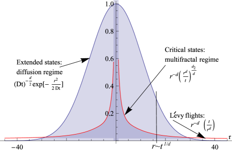
The Fourier transform $\hat{{\cal D}}_{r,r^{\prime}}(t)$ of this correlation function (“generalized diffusion propagator”) describes spreading of the wave packet in space and time and is a direct generalization of the pure classical object: the probability density to find a random walker at a point $r$ at a time $t$ after the beginning of random walk from the origin, $\,r^{\prime}=0$. The possibility of both classical and quantum formulation of the density correlation function makes this object convenient for quantum-to-classical comparison.

The descender of the generalized diffusion propagator is the survival probability or the return probability $P(t)$

$$2\pi\rho_{0}\,P(t)=\hat{{\cal D}}_{r,r}(t),$$ (2)

where $\rho_{0}$ is the averaged DoS.

This is the probability for a wave packet to survive for a time $t$ at a point where it was created at $t=0$ or the probability for a random walker to find himself in the origin at a time $t$. For extended states $P(t)$ decreases with time, albeit differently for the truly extended states and the critical multifractal states Chalker ; Chalker-proof :

$$P(t)\propto\left\{\begin{matrix}t^{-\frac{d}{2}},&{\rm extended\;\;\;states}\cr t^{-\frac{d_{2}}{d}},&{\rm critical\;\;\;states}\end{matrix}\right.$$ (3)

In Eq.(3), $d_{2}<d$ is the non-trivial critical exponent, the correlation fractal dimension, that determines inverse participation ratio in a critical system of the size $L$:

$${\cal I}_{2}=\left\langle\sum_{r}|\psi(r)|^{4}\right\rangle\propto L^{-d_{2}}.$$ (4)

A general form of the density correlation function, $\,{\cal D}(\kappa,\omega)$, was suggested by Chalker in the momentum-frequency representation Chalker ; Ch-D . In the region of critical states it can be written as follows:

$${\cal D}(\kappa,\omega)=\frac{2\pi\rho_{0}}{(-i\omega+0)\,[f(|\kappa|\,L_{-i\omega})+1]},$$ (5)

where $\rho_{0}=N^{-1}\sum_{n=0}^{N}\langle\delta(\varepsilon-\varepsilon_{n})\rangle|_{\varepsilon=0}$ is the averaged density of states at $\varepsilon=0$.

The key element of this prediction is that at criticality (in the classical Dyson symmetry classes) there is only one scale $1/L_{\omega}\propto\omega^{\frac{1}{d}}$ which separates small- and large-momentum behavior, both of them being different limits of one and the same analytic function $f(x)$. The combination $L_{-i\omega}\propto(-i\omega+0)^{-d}$ in Eq.(5) is dictated by the retarded character of the correlation function which should be a regular function in the upper half-plane of complex $\omega$.

Note that the original idea of Chalker was that of reconciling the one-parameter scaling of Gang-of-Four GoF with the multifractal behavior. The one-parameter scaling is encoded in Eq.(5): the counterpart of ${\cal D}(\kappa,\omega)$ in the coordinate-time domain obeys the scaling law

$$r^{d}\,\hat{{\cal D}}_{r,0}(t)=S(r^{d}/t)\,,$$ (6)

where $S(x)$ is the scaling function.

According to Chalker’s conjecture, the multifractality exhibits itself in the asymptotic form of the function $f(x)$ at $|x|\gg 1$:

$$f(x)=c\,x^{d_{2}},\;\;\;\;\;|x|\gg 1.$$ (7)

Here $d_{2}$ is the same correlation fractal dimension defined by Eq. (4) which appears also in Eq. (3) as well as in the local density of states correlation function Ref.Chalker-proof . It determines the multifractal regime of the density correlation function (see Fig. 1) where

$$\hat{{\cal D}}_{r,0}(t)\propto r^{-d}\,\left(\frac{r^{d}}{t}\right)^{\frac{d_{2}}{d}},\;\;\;\;\;(t>r^{d})\,.$$ (8)

At small $|x|\ll 1$, the function $f(x)$ is small as the probability conservation

$$\sum_{r^{\prime}}\hat{{\cal D}}_{r,r^{\prime}}(t)=2\pi\rho_{0}\,\theta(t)$$ (9)

requires

$$f(x=0)=0\,.$$ (10)

Assuming that $x=0$ is the regular point of the analytic function $f(x)$, one can expand

$$f(x)=c_{1}\,x+c_{2}\,x^{2}+c_{3}\,x^{3}+...,\;\;\;\;(x=|\kappa|\,L_{-i\omega}).$$ (11)

Note, however, that the regular expansion in $x$, Eq.(11), does not mean analyticity in the momentum domain. For instance the linear in $x$ term contains non-analytic term $|\kappa|$. Non-analytic in $\kappa$ terms arise from any odd power of $x$. These terms imply power-law tails of the density correlation function in the coordinate domain. Namely, if the leading odd term in Eq. (11) is $x^{2m-1}$, the density correlation function acquires a power-law tail $\propto r^{-(2m-1+d)}$ at large $r$. By analogy with classical random walks, we will refer to such tails as the Lévy flights.

The simplest class of critical systems, where such non-analytic terms are present, includes the systems with long-range resonance hopping where the hopping terms of the Hamiltonian decrease with distance as:

$$|\hat{H}_{r,r^{\prime}}|\propto|r-r^{\prime}|^{-d}.$$ (12)

However, the situation depends a lot on the dimensionality $d$. As we will show below, the Lévy flights in such systems are characterized by a power-law tail:

$$\hat{{\cal D}}_{r,0}(t)\propto r^{-d}\,\left(\frac{t}{r^{d}}\right),\;\;\;\;\;(t<r^{d})\,.$$ (13)

For $d=3$, the second moment $\langle r^{2}\rangle$ does exist so that we have in Eq. (11) that $c_{1}=0$ and $c_{2}$ is finite. The non-analytic in ${\kappa}$ terms appear starting from $x^{3}$, which, however, is sub-leading at small $x$. The role of non-analyticity is greatly enhanced at $d=1$ where $c_{1}\neq 0$. Here the leading term in Eq. (11) is non-analytic in $\kappa$. The case $d=2$ is special EfAl . In this case even criticality is not guaranteed by Eq. (12) and the answer may depend on the particular symmetry class and details of the Hamiltonian.

In this paper, we concentrate on the simplest system which belongs to the class of long-range random Hamiltonians, Eq. (12), with $d=1$. This is the ensemble of Hermitian critical power-law banded random matrices MFSeil (CPLBRM) where the multifractality can be continuously tuned from weak to strong by changing only one parameter $0<b<\infty$:

$$\langle H_{nm}\rangle=0,\;\;\;\langle|H_{nm}|^{2}\rangle=\left\{\begin{matrix}\beta^{-1},&n=m\cr\frac{1}{2\left[1+\left(\frac{n-m}{b}\right)^{2}\right]},&n\neq m\end{matrix}\right.,$$ (14)

where $\beta=1,2,4$ is the Dyson symmetry number.

We consider the limit of strong multifractality $b\ll 1$ and demonstrate the validity of Eqs. (5), (7), (8), (11) and (13) which are the key relationships for the description of Lévy flights and multifractality. Furthermore, we will find the function $f(x)$ explicitly for the Gaussian Orthogonal (GOE) and Unitary (GUE) ensembles thereby unifying both concepts of multifractality and Lévy flights in the one single analytic function.

One of the purposes of this paper is to compare the density correlations function for random critical states of a long-range Hamiltonian with that for the classical random walks on a fractal. For a classical random walk with a constant step length on a lattice the density correlation function decreases exponentially at large distances $\hat{{\cal D}}_{r,r^{\prime}}(t)\propto e^{-\frac{r^{2}}{2Dt}}$ and thus all moments $\langle r^{2m}\rangle$ are well defined. A peculiar class of random walks called “Lévy flights” is realized in the models with variable step length. If the probability to have a long step is heavily tailed, the probability distribution of random walks may have power-law tails at large distances and thus the moments $\langle r^{2m}\rangle$ may diverge Huges . The similar power-law tails may appear in classical random walk on hierarchical manifolds Wegner-1 ; Wegner-long ; ret-prob , where fractality is build in their geometry.
We will demonstrate that certain models of classical random walk on a fractal result in the same regimes of the density correlation function as for the quantum critical long-range Hamiltonians of Eq. (12). Namely, the two principle regimes Eqs. (8), (13) described in Fig. 1 have their counterparts for the classical diffusion, with the correlation fractal dimension $d_{2}$ being replaced by the Hausdorff dimension $d_{h}$ and the dimensionality of space $d$ being replaced by the walk dimension. Moreover, we will see that the critical exponent $2/d$ of sub-diffusion $\langle r^{2}\rangle\propto t^{2/d}$ for critical random Hamiltonians in $d>2$ dimensions appears to have the same relationship with the exponent $-d$ of Lévy flights $r^{d}\,\hat{{\cal D}}_{0,r}(t)\equiv S(r,t)\propto r^{-d}$ for the quantum problem with long-range random Hamiltonians, Eq. (12), and for the certain classical random walks on fractals Wegner-1 ; Wegner-long ; ret-prob .
The paper is organized as follows. In Section II we review the method of virial expansion in the number of resonant levels and give general expressions for the density correlation function (effective diffuson) for any almost diagonal Gaussian Random Matrix Theory (RMT). In Section III, we apply these expressions to compute the density correlation function for the specific CPLBRM in the coordinate/time representation and uncover multifractality and Lévy flights as consequences of the long-range nature of the Hamiltonian, Eq. (14). In Section IV, we compute the density correlation function in the coordinate/frequency representation. Sections V and VI are devoted to verification of the key relationships Eqs. (5), (7) and (11) due to multifractality and Lévy flights as seen in the momentum-frequency representation of the density correlation function. We explain a perturbative derivation of Lévy flights for strong multifractality and the Wigner-Dyson limit of the CPLBRM in Sections VII and VIII, respectively. In Section IX, we present numerical results for the critical RMT with weak and strong multifractality. In Section X, we discuss the classical random walks on fractals and show that in certain models they have the same phenomenology as their quantum counterpart. In Section XI we summarize the main results of the paper and discuss their applicability to the Anderson transition in 3D systems.

II Virial expansion method

In order to check the validity of Eqs. (5), (7), (8) (11) and (13) for the ensemble of CPLBRM, Eq. (14), at strong multifractality, $b\ll 1$, we exploit the method of virial expansion in the number of resonant levels KYevOss ; YevOss . This method is a certain re-summation of the locator expansion Anderson in the hopping matrix element $h_{nm}$:

$$h_{nm}^{2}=\langle|H_{n\neq m}|^{2}\rangle=\frac{1}{2}\,\frac{b^{2}}{(n-m)^{2}}.$$ (15)

The summation is organized so that any correlation function $C(\kappa,\omega)$ is represented as a series in $b\ll 1$:

$$C(\kappa,\omega)=\omega^{\eta}\sum_{m=1}^{\infty}b^{m-1}C^{(m)}(\kappa L_{\omega})\,,$$ (16)

where the length scale $L_{\omega}$ is itself $b$-dependent:

$$L_{\omega}=\frac{2\sqrt{2}b}{\omega\,\beta},$$ (17)

and $\eta$ is specific to a particular correlation function.

The advantage of this representation is that Eq. (16) is a functional series, each function $C^{(m)}(\kappa L_{\omega})$ adding details of correlations which emerge from resonant interaction of $m$ states. These states have energy levels $\varepsilon_{m}$ being anomalously close to each other within the interval of order $b\ll 1$. At small $b$, such “multiple collision” of levels has small probability. Therefore, even the few first terms in the series Eq. (16) give a very good approximation of the correlation function.

Note that the density of states $\rho_{E}\approx\sqrt{\frac{\beta}{2\pi}}\,e^{-\beta\,E^{2}/2}$ corresponding to CPLBRM Eq. (14) has negligible variation at a scale $E\sim b\ll 1$ [OurDOS, ]. We will neglect such variations throughout the paper and approximate $\rho(E)\approx\rho(0)=\rho_{0}$. With such an accuracy we obtain for the retarded density correlation function:

$$\tilde{{\cal D}}_{r,r^{\prime}}(\omega)=\frac{2\pi\rho_{0}}{-i\omega+0}\,\left[\delta_{r,r^{\prime}}+\tilde{{\cal D}}^{(2)}_{r,r^{\prime}}(\omega)+\tilde{{\cal D}}^{(3)}_{r,r^{\prime}}(\omega)+\ldots\right].$$ (18)

In Eq. (18) we denote

$$2\pi\rho_{0}\tilde{{\cal D}}_{r,r^{\prime}}^{(2,3)}(\omega)=\int_{0}^{\infty}e^{i\omega t}\,\partial_{t}\hat{{\cal D}}_{r,r^{\prime}}^{(2,3)}(t)\,dt.$$ (19)

The density correlation function in the time domain is given by:

$$\hat{{\cal D}}_{r,r^{\prime}}(t)\simeq\left(2\pi\rho_{0}\,\delta_{r,r^{\prime}}\,+\hat{{\cal D}}^{(2)}_{r,r^{\prime}}(t)+\hat{{\cal D}}^{(3)}_{r,r^{\prime}}(t)\right){\theta(t)}\,.$$ (20)

To simplify formulae, we assume below $\,t>0\,$ and skip $\,\theta(t)$.

Calculating leading terms of the virial expansion, we obtain the following expressions for $\beta=1$ (GOE):

$$\hat{{\cal D}}^{(2)}_{r\neq r^{\prime}}(t)=2\pi h_{r,r^{\prime}}^{2}\,t\,e^{-(h_{r,r^{\prime}}t)^{2}}\,I_{0}\Bigl{(}(h_{r,r^{\prime}}t)^{2}\Bigr{)}\,;$$ (21)

and for $\beta=2$ (GUE):

$$\hat{{\cal D}}^{(2)}_{r\neq r^{\prime}}(t)=2\pi\left[h_{r,r^{\prime}}^{2}\,t\,e^{-(h_{r,r^{\prime}}t)^{2}}+\frac{\sqrt{\pi}}{2}\,h_{r,r^{\prime}}\,{\rm Erf}(h_{r,r^{\prime}}t)\right]\,,$$ (22)

where $h_{r,r^{\prime}}$ is defined in Eq. (15); $\,I_{j}(\ldots)\,$ is the modified Bessel function of the first kind. Answers for subleading terms of the virial expansion are more lengthy and we will publish them elsewhere 3col .

Equations (18)-(22) are valid for any Gaussian RMT with an arbitrary variance $h_{r,r^{\prime}}^{2}$ of the hopping matrix elements that is parametrically smaller than the variance of the diagonal ones (almost diagonal Gaussian RMT).

Remarkably, $\hat{{\cal D}}^{(2,3)}_{r,r^{\prime}}(t)$ at $r=r^{\prime}$ is expressed in terms of $\hat{{\cal D}}^{(2,3)}_{r\neq r^{\prime}}(t)$ as follows:

$$\hat{{\cal D}}^{(m)}_{r,r}(t)=-\sum_{r\neq r^{\prime}}\hat{{\cal D}}^{(m)}_{r,r^{\prime}}(t)\,,\ m=2,3.$$ (23)

This is a consequence of the particle conservation which requires

$$\sum_{r}\hat{{\cal D}}_{r,r^{\prime}}(t)=2\pi\rho_{0}\,.$$ (24)

As this relation is already fulfilled by the first term in Eq. (18), all other terms proportional to ${\cal D}_{r,r^{\prime}}^{(m)}$ ($m\geq 2$) should obey Eq. (23).

III Density correlation function in the time domain and return probability

An inspection of Eqs. (21), (22) shows that for the CPLBRM with $b\ll 1$ the asymptotic behavior of the effective diffuson $\hat{{\cal D}}_{r,r^{\prime}}(t)=\rho_{0}^{-1}\,\hat{{\cal D}}_{r,r^{\prime}}^{(2)}(t)$ is given by:

$$\hat{{\cal D}}_{r,r^{\prime}}(t)=2\pi\rho_{0}\left\{\begin{matrix}\frac{\sqrt{2}\,b}{2|r-r^{\prime}|},&{\rm GOE}\cr\frac{\pi\,b}{2\sqrt{2}|r-r^{\prime}|},&{\rm GUE}\end{matrix}\right.,\;\;\;\;|r-r^{\prime}|\ll b\,t\,.$$ (25)

$$\hat{{\cal D}}_{r,r^{\prime}}(t)=\frac{\pi\beta\,b^{2}\,t}{\,|r-r^{\prime}|^{2}},\;\;\;\;|r-r^{\prime}|\gg b\,t\,.$$ (26)

In a more general case of long-range Hamiltonians obeying Eq. (12) one should replace $|r-r^{\prime}|\rightarrow|r-r^{\prime}|^{d}$ to obtain the large-distance tail Eq. (13) which is the hallmark of the Lévy flights.

The small-distance behavior $\hat{{\cal D}}_{r,r^{\prime}}(t)\propto|r-r^{\prime}|^{-d}$ is also remarkable. Applying Eq. (23) one obtains for the survival probability Eq. (2):

$$P(t)=1-\frac{d_{2}}{d}\,\ln(b\,t)\approx(b\,t)^{-\frac{d_{2}}{d}},$$ (27)

(see Ref.[Chalker-proof, ] for more details) where for the CPLBRM one finds Mirlin-rev :

$$\frac{d_{2}}{d}\simeq\left\{\begin{matrix}\sqrt{2}\,b,&{\rm GOE}\cr\frac{\pi\,b}{\sqrt{2}},&{\rm GUE}\end{matrix}\right.,\;\;\;\;(b\ll 1)\,.$$ (28)

Thus Eq. (27) shows that the asymptotic behavior $|r-r^{\prime}|^{-d}$ is a signature of (strong) multifractality with the correlation dimension given by Eq. (28).

We conclude this section by emphasizing once again that the multifractality and Lévy flights for the long-range Hamiltonians Eq. (12) have the same root and cannot exist one without the other.

IV Density correlation function in the frequency domain

One can invert Eq. (19) and obtain:

$$\tilde{{\cal D}}_{r\neq r^{\prime}}(\omega)=\frac{\sqrt{2\pi}\beta^{\frac{3}{2}}\pi^{\beta-1}}{4}\,\frac{i}{z}\,\Omega^{(\beta)}(z),$$ (29)

where

$$z=(|r-r^{\prime}|/L_{\omega})^{d}\propto\omega\,|r-r^{\prime}|^{d}\,,$$ (30)

$d=1\,$ for CPLBRM, $L_{\omega}$ is given by Eq. (17) and expressions for $\,\Omega\,$ read:

$$\Omega^{({\rm GOE})}(z)=z^{2}e^{-z^{2}}\,\left[\left(K_{0}(z^{2})+K_{1}(z^{2})\right)\right.+$$

$$\left.\pi i\,{\rm sgn}(z)\,\left(I_{0}(z^{2})-I_{1}(z^{2})\right)\right],\;\;\;({\rm GOE},\beta=1)\,;$$ (31)

$$\Omega^{({\rm GUE})}(z)=(z^{2}+\frac{1}{2})e^{-z^{2}}\times$$ (32)

$$\left[1+i\,\left({\rm Erfi}(z)-\frac{z\,e^{z^{2}}}{\sqrt{\pi}\,(z^{2}+\frac{1}{2})}\right)\right],\;\;\;({\rm GUE},\beta=2)\,;$$

$\,K_{j}(\ldots)\,$ is the modified Bessel function of the second kind. Functions $\Omega^{(\beta)}(z)$ in Eqs. (IV), (32) are qualitatively very similar for the orthogonal and the unitary ensemble (see Figs. 2,3).

Figure 2: (color online) Real part of the functions $\Omega^{({\rm GOE})}(z)$ in Eq. (IV) (blue) and $\Omega^{({\rm GUE})}(z)$ in Eq. (32) (red). They describe the $\omega$-dependence of the corrections $\tilde{{\cal D}}^{(2)}_{r,r^{\prime}}$ to the retarded density correlation function at a fixed $r\neq r^{\prime}$. Note that these corrections are caused by the extended nature of wave functions.

Figure 3: (color online) Imaginary part of the functions $\Omega^{({\rm GOE})}(z)$ in Eq. (IV) (blue) and $\Omega^{({\rm GUE})}(z)$ in Eq. (32) (red).

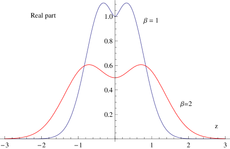
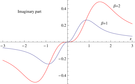
Their real parts are even functions of $z$ which exponentially decrease like $|z|^{\beta}\,e^{-2z^{2}/\beta}$ at $|z|\gg 1$. The imaginary parts are odd functions of $z$ which behave like $z^{-1}$ at large $|z|$. Correspondingly, the density correlation function in the coordinate-frequency representation behaves at $|z|\gg 1$ (large distances or frequencies) like:

$${\rm Im}[\tilde{{\cal D}}_{r\neq r^{\prime}}(\omega)] \sim {\rm sign}(z)\,|z|^{\beta-1}\,e^{-2z^{2}/\beta},$$ (33)

$${\rm Re}[\tilde{{\cal D}}_{r\neq r^{\prime}}(\omega)] \sim -\frac{1}{z^{2}}.$$ (34)

Note that the correlation function $\tilde{{\cal D}}_{r\neq r^{\prime}}(\omega)$ for $|r-r^{\prime}|\gg L_{\omega}$ has a power-law tail. This is another manifestation of Lévy flights in the $r-\omega$ domain.

V Frequency-momentum representation.

Now we compute the retarded density correlation function ${\cal D}(\kappa,\omega)$ in the momentum-frequency representation. This allows us to make contact with Eq. (5) to check Chalker’s conjecture on the effect of multifractality Eq. (7) and to detect the non-analytic in $\kappa$ terms in Eq. (11), which is a signature of Lévy flights.

To this end we define:

$${\cal D}^{(2)}(\kappa,\omega)=\frac{1}{N}\sum_{r,r^{\prime}}\tilde{{\cal D}}_{r,r^{\prime}}^{(2)}(\omega)\,e^{i\kappa\,(r-r^{\prime})},$$ (35)

where $N\times N$ is the size of the matrix. We assume this size to be larger than all the relevant length scales of the system. If in addition $\kappa\ll 1$, one can switch from the sum to integral in Eq. (35) to implement the continuous approximation which is valid at $|L_{\omega}|\gg 1$.

Before proceeding with calculations, let us note that Eq. (23) implies:

$${\cal D}^{(2)}(\kappa=0,\omega)=0.$$ (36)

Thus one can do the Fourier transform of $\tilde{{\cal D}}^{(2)}_{r,r^{\prime}}(\omega)$ at $|r-r^{\prime}|\neq 0$ and then subtract the $\kappa=0$ value of the result obtained. Thus, we obtain from Eqs. (IV), (32):

$${\cal D}(\kappa,\omega)=\frac{2\pi\rho_{0}}{-i\omega+0}+|L_{\omega}|\,G(\bar{\kappa}),$$ (37)

where $\bar{\kappa}=\kappa\,L_{\omega}$. One can easily see that Eq. (37) is consistent with Eq. (5) in the limit $\,b\log(\bar{k})\ll 1$, with $\,f(x)=i(\sqrt{2}/\pi\beta\rho_{0})\,b\,G(\bar{k})$. The retarded character of the correlation function is encoded in real and imaginary parts of $\,G(\bar{k})\,$ which obey the Kramers-Kronig relationship. The expressions for them read

GOE, $\,\beta=1$:

$${\rm Re}[G^{({\rm GOE})}(\bar{\kappa})]=\frac{(2\pi)^{2}}{32}\,|\bar{\kappa}|\,e^{-\frac{\bar{\kappa}^{2}}{16}}\,I_{0}\left(\frac{\bar{\kappa}^{2}}{16}\right),$$ (38)

$${\rm Im}[G^{({\rm GOE})}(\bar{\kappa})]=-{\rm sign(\omega)}\frac{\sqrt{2\pi}}{4}\times$$

$$\left[1+\frac{\bar{\kappa}^{2}}{3}\,{\rm pFq}\left(\{1,1,3\},\left\{\frac{3}{2},2,\frac{5}{2}\right\},-\frac{\bar{\kappa}^{2}}{8}\right)\right.-$$

$$\left.{\rm pFq}\left(\{1,1\},\left\{\frac{1}{2},\frac{3}{2}\right\},-\frac{\bar{\kappa}^{2}}{8}\right)\right],$$ (39)

GUE, $\,\beta=2$:

$${\rm Re}[G^{({\rm GUE})}(\bar{\kappa})]=\frac{\pi^{2}}{2}\,\left[|\bar{\kappa}|\,e^{-\frac{\bar{\kappa}^{2}}{4}}-\sqrt{\pi}\,{\rm Erf}\left(\frac{\bar{\kappa}}{2}\right)\right].$$ (40)

$${\rm Im}[G^{({\rm GUE})}(\bar{\kappa})] = -{\rm sign(\omega)}\frac{\pi^{\frac{3}{2}}}{4}\,\left[2\sqrt{\pi}\,e^{-\frac{\bar{\kappa}^{2}}{4}}\,\bar{\kappa}\,{\rm Erfi}\left(\frac{\bar{\kappa}}{2}\right)+\right.$$ (41)

$$\left.\bar{\kappa}^{2}\,{\rm pFq}\left(\{1,1\},\left\{\frac{3}{2},2\right\},-\frac{\bar{\kappa}^{2}}{4}\right)\right]\,.$$

Here $\gamma$ is the Euler constant and ${\rm pFq}(...)$ is the hypergeometric function. We discuss these results in the next section.

VI Comparison with the Chalker’s conjecture.

The asymptotic behavior of the functions $G^{{\rm GOE}}(\bar{\kappa})$ and $G^{{\rm GUE}}(\bar{\kappa})$ is very similar. At small $\bar{\kappa}\ll 1$:

$${\rm Re}[G(\bar{\kappa})]=\left\{\begin{matrix}\frac{1}{2}\pi^{2}\,|\bar{\kappa}|,&\beta=1\cr\pi^{2}\,|\bar{\kappa}|,&\beta=2\end{matrix}\right.\,,$$ (42)

$${\rm Im}[G(\bar{\kappa})]=\left\{\begin{matrix}-\frac{1}{4}\sqrt{\frac{\pi}{2}}\,\bar{\kappa}^{2},&\beta=1\cr-\frac{3}{8}\,\bar{\kappa}^{2},&\beta=2\end{matrix}\right.\,.$$ (43)

This is consistent with Eq. (11) (at $d=1$) where all $c_{i}\sim b$. In particular, the non-analytic behavior $\propto|\bar{\kappa}|$ caused by the Lévy-flights is confirmed by Eq. (42). Eq. (43) corresponds to corrections $\propto c_{2}\,x^{2}$ in Eq. (11).

Figure 4: (color online) Real part of $G(\bar{k})$ for ${\rm GOE}$ (blue) and GUE (red). The dashed lines is the asymptotic behavior given by Eq. (11) (red) and Eq. (7) (black) at $d_{2}=0.01$ and $c=1+O(b)$. For better comparison the GUE curve is given in the re-scaled coordinates so that the asymptotic behavior at small and large $\kappa$ coincides with that of the GOE curve.

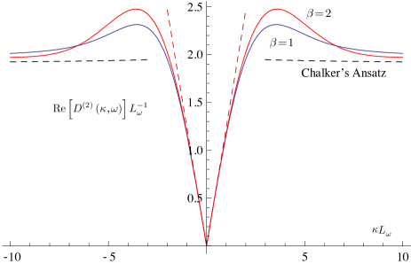
More interesting is the asymptotic behavior of $G(\bar{k})$ at large $|\bar{\kappa}|\gg 1$. While ${\rm Re}[G(\bar{\kappa})]$ tends to a constant

$${\rm Re}[G(\bar{\kappa})]=\left\{\begin{matrix}\frac{\pi^{\frac{3}{2}}}{2\sqrt{2}},&\beta=1\cr\frac{\pi^{\frac{5}{2}}}{2},&\beta=2\end{matrix}\right.\,\,\,\;\;\;(|\bar{\kappa}|\gg 1),$$ (44)

$|{\rm Im}[G(\bar{\kappa})]|$ increases logarithmically

$${\rm Im}[G(\bar{\kappa})]=\left\{\begin{matrix}-\frac{\sqrt{2\pi}}{2}\,\ln(|\bar{\kappa}|)+{\rm const},&\beta=1\cr-\frac{1}{2}\,\ln(|\bar{\kappa}|)+{\rm const},&\beta=2\end{matrix}\right.\,.$$ (45)

Such a behavior is fully consistent with Eq. (7), in which a sub-leading term is added:

$$f(x)=cx^{d_{2}}-c\,.$$ (46)

For very large $\,x\gg\exp(1/b)$, Eq. (46) reduces to Eq. (7) while in the intermediate region $\,1\ll x\ll\exp(1/b)$, which is present only at small $b\ll 1$, one obtains:

$$f(x)\simeq cd_{2}\log(x)\,.$$

Thus we confirm the Chalker’s conjecture for the density correlation function to the first order in the small parameter $b\ll 1$.

In order to illustrate the similarity of the density correlation functions conjectured in Eqs. (5), (7) and (11) and obtained analytically for the CPLBRM Eq. (14), we plot in Fig. 4 and Fig. 5 the real and imaginary parts of $G(\bar{\kappa})$ together with the asymptotic behavior Eq. (7) at a small $d_{2}=0.01$. The choice of only one constant, $c=1+O(b)$, ensures both the right leading logarithmic behavior of ${\rm Im}[G(\bar{\kappa})]$ and the correct limit of ${\rm Re}[G(\bar{\kappa})]$ as $\bar{\kappa}\rightarrow\infty$. It is also seen that upon a proper re-scaling of $x$ and $y$ coordinates the shape of $G^{{\rm GOE}}(\bar{\kappa})$ and $G^{{\rm GUE}}(\bar{\kappa})$ is very similar. We conclude therefore that the shape of the $G(\bar{\kappa})$ dependence is dictated mostly by criticality encoded in the Chalker’s conjecture and not by the symmetry of the Hamiltonian.

Figure 5: (color online) Imaginary part of $G(\bar{k})$ for GOE (blue) and GUE (red). The latter curve is given in the re-scaled coordinates as in Fig. 4. The black dashed line represents the asymptotic behavior Eq. (7) for the proper choice of the coefficient $c=1+0.90\,b$ and $d_{2}=0.01$.

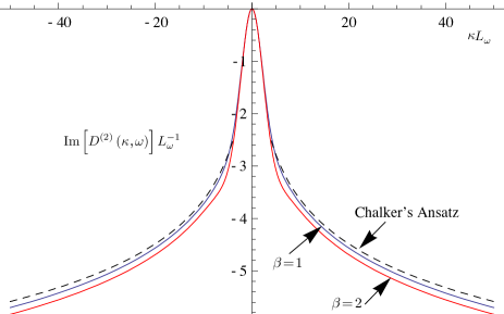
VII Lévy flights for strong multifractality: a poor-men derivation.

In this section, we exploit another expression for the density correlation function (at a fixed energy of the wave packet $\varepsilon$ which has been reinstated in this Section) in the time domain which is equivalent to Eq. (1) provided that $\omega\ll B$ or $t\gg 1/B$, where $B$ is the energy bandwidth:

$$\hat{{\cal D}}_{r,r^{\prime}}(t) = 2\pi\sum_{n,m}\langle\delta(\varepsilon-\varepsilon_{n})e^{it(\varepsilon_{m}-\varepsilon_{n})}$$

$$\psi_{n}(r)\psi_{n}^{*}(r+R)\psi_{m}(r+R)\psi_{m}^{*}(r)\rangle.$$

Note that $\hat{{\cal D}}_{r\neq r^{\prime}}(t=0)=0$ due to completeness of the set of normalized wave functions. Therefore, one can replace $e^{it(\varepsilon_{n}-\varepsilon_{m})}$ by $e^{it(\varepsilon_{n}-\varepsilon_{m})}-1$ without changing the result.

Let us consider very strong multifractality and very large distances $R=r-r^{\prime}$. Then the wave function can be approximated as

$$\psi_{n}(r\neq n)\approx\frac{H_{n,r}}{\varepsilon_{n}-\varepsilon_{r}},\;\;\;\;\psi_{n}(r=n)\approx 1,$$ (48)

where $H_{nm}$ is an off-diagonal entry of the matrix Hamiltonian and $\varepsilon_{n}\equiv H_{nn}$ is the diagonal entry. In the case of very small $b$, when the wave functions normalization is almost all concentrated at one site $n$ (center of localization), the eigenenergy of a state $\varepsilon_{n}$ is almost equal to the on-site energy $H_{nn}$.

The main contribution to Eq. (VII) is given by two terms $(m=r,n=r+R)$ or $(n=r,m=r+R)$. In both cases the combination of wave functions is equal to:

$$-\frac{|H_{r,r+R}|^{2}}{(\varepsilon_{r}-\varepsilon_{r+R})^{2}}\,.$$

Now, we average over disorder. For a Gaussian ensemble, averaging over $\varepsilon_{n}=H_{nn}$ and over the hopping matrix elements $H_{nm}$ are independent from each other. Therefore, we replace $|H_{nm}|^{2}$ by its average $\langle|H_{nm}|^{2}\rangle$ given by Eq. (14) and reduce averaging over $\varepsilon_{n}$ to the energy integral with the help of the spectral correlation function $R(\varepsilon,\varepsilon^{\prime})=\langle\rho(\varepsilon)\,\rho(\varepsilon^{\prime})\rangle$:

$$\hat{{\cal D}}_{r,r+R}(t)\approx\int_{-\infty}^{+\infty}d\varepsilon^{\prime}\,R(\varepsilon,\varepsilon^{\prime})\,\frac{1-e^{it(\varepsilon-\varepsilon^{\prime})}}{(\varepsilon-\varepsilon^{\prime})^{2}}\,\frac{2\pi\,b^{2}}{R^{2}}\,.$$ (49)

Note that due to level repulsion $R(\varepsilon,\varepsilon)=0$ the integral in Eq. (49) is convergent at $\varepsilon^{\prime}=\varepsilon$. However, at $\,t\,$ being smaller than the Heisenberg time, $t\ll t_{{\rm H}}=N\rho_{0}$ (or $\omega\gg\Delta\sim B/N$), the region of level repulsion is very narrow so that one can replace $R(\varepsilon,\varepsilon^{\prime})\approx\rho(\varepsilon)\rho(\varepsilon^{\prime})$, where $\rho(\varepsilon)$ is the averaged DoS. Using also the symmetric form of the averaged DoS $\rho(\varepsilon)=\rho(-\varepsilon)$ we obtain at $\varepsilon=0$:

$$\hat{{\cal D}}_{r,r+R}(t)\approx\frac{4\pi\rho_{0}\,b^{2}}{R^{2}}\int_{0}^{+\infty}d\varepsilon^{\prime}\,\rho(\varepsilon^{\prime})\,\frac{1-\cos(t\varepsilon^{\prime})}{\varepsilon^{\prime 2}}.$$ (50)

At $t\gg 1/B$, the integral in Eq. (50) is dominated by $\varepsilon^{\prime}\ll B$ and one can replace $\rho(\varepsilon^{\prime})\approx\rho_{0}$ and obtain:

$$\hat{{\cal D}}_{r,r+R}(t)\approx\frac{4\pi\rho_{0}^{2}\,b^{2}}{R^{2}}\,t\int_{0}^{+\infty}dx\,\frac{1-\cos(x)}{x^{2}}=\frac{2\pi^{2}\rho_{0}^{2}\,b^{2}}{R^{2}}\,t\,.$$ (51)

This is exactly the result Eq. (26) obtained in the corresponding limit $R\gg bt$ from general formulae of the virial expansion.

Note, however, that Eq. (51) does not describe the behavior of the correlation function Eq. (VII) at smallest $t\ll\rho_{0}\sim 1/B$. In this case, one can expand the exponent in Eq. (50) and arrive at:

$$\hat{{\cal D}}_{r,r+R}(t)\approx\frac{2\pi\rho_{0}\,b^{2}}{R^{2}}\,t^{2}\int_{0}^{+\infty}dx\rho(x)=\frac{\pi\rho_{0}b^{2}}{R^{2}}\,t^{2}.$$ (52)

The two asymptotics Eq. (51) and Eq. (52) match each other at $t\sim\rho_{0}$. They both describe the Lévy flights. However, Eq. (51) has the scaling form $R^{-d}\,(t/R^{-d})$ (at $d=1$) while Eq. (52) is the fully perturbative result which violates the critical scaling law $\hat{{\cal D}}_{r,r+R}(t)=R^{-d}\,S(R^{d}/t)$. In the macroscopic thermodynamic limit, when $R\rightarrow\infty$, $t/R^{d}$ fixed but $R/L\rightarrow 0$, the perturbative region plotted as a function $t/R^{d}$ shrinks to zero.

VIII Density correlation function in the Wigner-Dyson limit $\,b\to\infty$

One can consider another limit when the size of the system $L=N$ is fixed and the parameter $b$ in Eq. (14) is increasing. The limit $b\rightarrow\infty$ corresponds to the Wigner-Dyson RMT. In this limit, the system becomes effectively zero dimensional and is not critical any longer. Nevertheless, we derive and briefly review its density correlation function for the sake of completeness.

We start with the same Eq. (VII) as in the previous section but employ the independent averaging over eigenvalues and eigenfunctions. The former is given by the famous Wigner-Dyson statistics Mehta while the latter is described by the Porter-Thomas statistics. The simplest case is $\beta=2$ when the eigenfunction $\psi_{n}(r)\equiv U_{nr}$ is uniformly distributed over the unitary group ${\cal U}(N)$. The averages of the products of $\psi$-functions are well known, e.g.:

$$\langle U_{nr_{1}}U_{n^{\prime}r_{2}}^{*}U_{mr_{2}^{\prime}}U_{m^{\prime}r_{1}^{\prime}}^{*}\rangle=\frac{1}{N^{2}-1}$$ (53)

$$(\delta_{nn^{\prime}}\delta_{r_{1}r_{2}}\delta_{mm^{\prime}}\delta_{r_{1}^{\prime}r_{2}^{\prime}}+\delta_{nm^{\prime}}\delta_{r_{1}r_{1}^{\prime}}\delta_{mn^{\prime}}\delta_{r_{2}r_{2}^{\prime}})-$$

$$\frac{1}{N(N^{2}-1)}(\delta_{nn^{\prime}}\delta_{r_{1}r_{1}^{\prime}}\delta_{mm^{\prime}}\delta_{r_{2}^{\prime}r_{2}}+\delta_{nm^{\prime}}\delta_{r_{1}r_{2}}\delta_{mn^{\prime}}\delta_{r_{2}^{\prime}r_{1}^{\prime}}).$$

Using Eq. (53), we obtain:

$$(2\pi\rho_{0})^{-1}\,\hat{{\cal D}}_{r,r+R}(t)=\delta_{R,0}+(K(t)-N)\,\frac{\delta_{R,0}N-1}{N^{2}-1},$$ (54)

where $K(t)$ is the spectral form-factor:

$$K(t)=\frac{1}{N\rho_{0}}\,\sum_{n,m}\langle\delta(\varepsilon-\varepsilon_{n})\,e^{it(\varepsilon_{m}-\varepsilon_{m})}\rangle.$$ (55)

At $t=0$, summations over $n$ and $m$ are independent and one finds $K(t=0)=N$ while at large $t\rightarrow\infty$ only terms with $n=m$ survive and $K(t\rightarrow\infty)=1$. However, the behavior of $K(t)$ at small times is highly uneven: $K(t)$ drops to almost zero for a very short time of the order of the inverse bandwidth $\rho_{0}\sim 1/B\propto 1/\sqrt{N}$ and then it recovers to unity; for example, in the unitary ensemble Mehta : $\,K=t/t_{{\rm H}}\,$ for $\rho_{0}\ll t<t_{{\rm H}}$ and $\,K=1$ for $\,t>t_{{\rm H}};$ we remind that the Heisenberg time is $t_{{\rm H}}=N\rho_{0}$.

One can immediately see that at $t=0$ Eq. (54) is the discrete $\delta$-function $\delta_{R,0}$ and that the sum rule Eq. (9) is fulfilled at any $t$. Furthermore, the density correlation function remains a combination of a $\delta$-function and a flat background at any $t$. The weight of the $\delta$-function determines the return probability:

$$P(t)=1-\frac{N}{N^{2}-1}\,(N-K(t)).$$ (56)

The non-monotonic behavior of $K(t)$ results in the similar behavior of the return probability: for a short time $t\sim\rho_{0}\sim 1/\sqrt{N}$, the wave packet leaves the origin almost completely. However, at later times it accumulates again in the origin reaching the value $P(t)=\frac{1}{N+1}$ at $t>t_{{\rm H}}$. Such an echo behavior is typical for a chaotic quantum system of finite size.

The flat background behaves with time as

$$2\pi\rho_{0}\,\hat{{\cal D}}_{r,r+R}(t)=\frac{N-K(t)}{N^{2}-1},\;\;\;\;(R>0).$$ (57)

It rapidly grows at small times, then decreases a bit and reaches the constant limit $1/(N+1)$ at $t>t_{{\rm H}}$.

Despite all unevenness of the behavior discussed above, there is one rough feature: at finite $R$ the flat background is always small like $N^{-1}$. Given that the critical Hamiltonian Eq (12) approaches the Wigner-Dyson RMT at $b\rightarrow N$, one expects the density correlation function to decrease at constant (large) system size $N$ as the parameter $b>1$ increases.

IX Numerical results

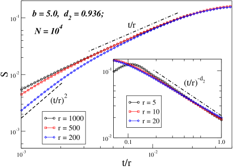
In order to check the analytical results of the previous sections and, more importantly, in order to verify their robustness for long-range critical random matrix models with weak multifractality, we performed statistical analysis of eigenvalues and eigenfunctions obtained by direct diagonalization of large matrices drawn from the Gaussian orthogonal ensemble Eq. (14) with $\,\beta=1$. The results are summarized in Fig. 6 and Fig. 7.

Figure 6: (color online) Scaling function $S=r\,\hat{{\cal D}}_{r^{\prime},r^{\prime}+r}(t)$ averaged over $r^{\prime}$ for different fixed $r=100,200,500,1000$ for the long-range critical random matrix ensemble Eq. (14) with $\,\beta=1,\ b=0.1\,$ and the matrix size $N=10^{4}$. The curves for the multifractal regime Eq. (8) and for the Lévy flights Eq. (13) collapse to the one single scaling curve. The perturbative Lévy flights Eq. (52) at the smallest $t$ do not obey the scaling.

Figure 7: (color online) Scaling function $S=r\,\hat{{\cal D}}_{r^{\prime},r^{\prime}+r}(t)$ averaged over $r^{\prime}$ for different fixed $r$ for the long-range critical random matrix ensemble Eq. (14) with $\,\beta=1,\ b=5\,$ and the matrix size $N=10^{4}$. Main plot: $r=200,500,1000$. The region of Lévy flights with scaling Eq. (13) shrinks compared to the case of small $b=0.1$. The region of perturbative Lévy flights Eq. (52) increases with decreasing $r$. Inset: the same scaling function for small $r=5,10,20$ and larger values of $t/r$. The multifractal regime, Eq. (8), is well seen and it crosses over directly to the perturbative Lévy flights, Eq. (52), at small $t/r$.

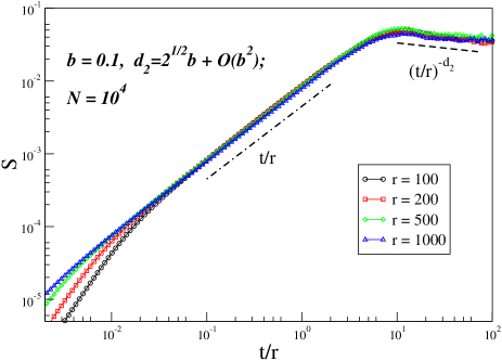
In Fig. 6, we demonstrate the scaling Eq. (6) in the two main scaling regimes Eqs. (8), (13) for the case of strong multifractality $b=0.1$. Both the multifractal regime of Chalker and the Lévy flights $\propto t/r^{2}$ are well seen and the scaling Eq. (6) is confirmed by a collapse of curves for several values of the distances $r$ to the one single scaling curve. The scaling Eq. (6) is violated at very small $t<\rho_{0}$ where inhomogeneity of spectrum (finite size effects in the energy space) should be taken into account and Eq. (52) stands for Eq. (13). Another possible source of violation of scaling is the finite-size effects in the coordinate space which exhibit themselves as the corrections in the parameter $r^{d}/N\ll 1$ and are important at not very small $r^{d}/N$.

In Fig. 7, we show the critical density correlation function for weak multifractality in the case $b>1$. Besides the scaling and the Chalker’s ansatz for the power-law behavior Eq. (8) in the multifractal region, the focus of our study was the power-law tail at small $t/r$ that describes the Lévy flights. It is seen that the region of the “scaling” Lévy flights Eq. (13) is much more narrow for $b>1$ compared to the case of small $b$ and is shrinking as $r$ decreases. However, the exponent $p$ of the power-law in the scaling function $S(x)\propto x^{-p}$, ($x\gg 1$) stays constant $p=1$ and independent of the strength of multifractality, i.e. of the parameter $b$. This result is not obvious for large $b$ where the arguments behind the derivation of Eq. (51) no longer apply. It was also verified analytically by considering the next order in the virial expansion 3col . In the next section, we will consider the classical analogue of such a behavior.

X Random walks over hierarchical manifold with level-dependent asymmetric rate

In Ref.[Wegner-1, ] Wegner and Grossmann (WG) suggested a classical random walk process on an hierarchical structure that is rich enough to mimic many relevant regimes in transport in disordered systems and in fluid turbulence. Its rigorous definition is given in the original work. Here we illustrate this process for the 2d Sierpinski gasket, see Fig. 8. As any regular fractal, the Sierpinski gasket is characterized by the hierarchy of self-similar clusters, each one containing $z$ clusters of the next generation (level). For the Sierpinski gasket of Fig. 8 $z=3$. Another important parameter of the fractal geometry is the space scaling factor $\mu>1$ that is the ratio of linear sizes of the clusters of the $k$-th and the $k+1$-th levels. For the Sierpinski gasket of Fig. 8 $\mu=2$. As in the original work [Wegner-1, ], we assume that there is a smallest level $k=0$ with the size of triangle equal to 1. Then, the size of the triangle of the largest level $k=l$ is $L=\mu^{l}$ and there are $z^{l}$ white triangles of the smallest level in it. The parameters $z$ and $\mu$ determine the Hausdorff fractal dimension, i.e. the exponent $d_{h}$ that governs the scaling $S\propto L^{d_{h}}$ of the total area of white triangles as the size of the largest triangle $L$ increases. Given that $S\propto z^{l}$, one immediately finds that

$$d_{h}=\frac{\ln z}{\ln\mu}.$$ (58)

Figure 8: (color online) The example of a 2d hierarchical manifold: jumps occur only between the full (colored) triangles of the neighboring generations (levels) shown by different colors. There are neither jumps between triangles of the same level (size), nor jumps between triangles that are not directly touching each other.

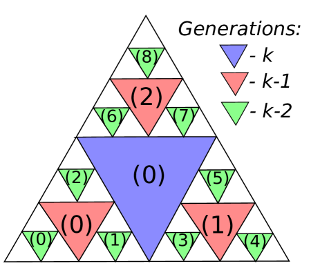
The WG random walk process can be viewed as jumps over the manifolds of centers of the full (colored) triangles each of them being determined by two numbers $(k,i)$, where $k$ is the level of the triangle and $i$ enumerates in a certain way (see Fig. 8) all the $z^{k-l}$ triangles of the given level $k$. An important rule is that a jump may occur only by one level up and by one level down. The up-jump may occur from each of $z$ smaller full triangles of the $k-1$ level to the one single larger triangle of the $k$-th level which smaller triangles touch directly. It happens with the rate:

$$W_{k}^{({\rm up})}=s^{k}.$$ (59)

The opposite process of down-jump is supposed to have a rate:

$$W_{k}^{({\rm down})}=\frac{s^{k}}{z\,r}.$$ (60)

The presence of $z$ in the denominator is natural as the down-jump happens to one of the $z$ smaller triangles that touch the larger triangle. What is the crucial invention of Wegner and Grossmann is the rate asymmetry parameter $r$. It is this parameter that makes the up-jumps (down-jumps) a predominant process if $r>1(<1)$.

The rate scaling parameter $s$ is natural on every hierarchical structure of the type Fig. 8 in order to compensate for the increasing length of jumps as the level increases. The ”normal” case is when $s<1$. In this case the Lévy flights cannot occur. On the other hand, if $s>1$ and $r=1$, all the moments $\langle x^{m}\rangle$ ($m>0$) of random walk displacement are divergent at all times. This is a somewhat pathological model.

The presence of the rate asymmetry parameter allows one to reach new regime (regime “C” in Ref.[Wegner-long, ]) at $r<1$ where $s>1$ but $(r\,s)<1$. It is exactly the regime where the density correlation function behaves similarly to that in the quantum case of random critical long-range Hamiltonians of Eq. (12). Note that the case $r<1$ and $s=1$ would result in trapping of a random walker on a fractal with no restriction to the level number from below. Indeed, in this case the bias towards down-jumps would drive the walker to lower and lower levels of hierarchy without a considerable displacement in the space. It is not the case in the WG model where the minimal level of hierarchy does exist, so after reaching it, the walker must go to the higher level with certainty and thereby may escape to arbitrary large distance. Thus, the coarse-grained WG model never leads to localization but only to sub-diffusion:

$$\langle x^{2}\rangle\propto t^{\Theta}\equiv t^{\frac{2}{d_{w}}},\;\;\;\;(\Theta<1).$$ (61)

In Eq. (61) we introduced the walk dimension $d_{w}$ which is essentially the dynamical exponent that determines the relative scaling of space and time. In the WG model with

$$s>1,\;\;\;\;\;sr<1,$$ (62)

it is given by Wegner-long :

$$d_{w}=\frac{\ln(sr)^{-1}}{\ln\mu}$$ (63)

and leads to a sub-diffusion $\Theta<1$ if $(sr)^{-1}>\mu^{2}$.

The definition Eq(61) is similar to the celebrated critical subdiffusion $\,\langle x\rangle^{2}\propto t^{2/d}\,$ which is well-known from the scaling theory of Anderson localization GoF . This suggests that $\,d_{w}\,$ in (61) has the same meaning as the dimensionality of space in the quantum critical models. Now we show that the WG random walk with the parameters $s$ and $r$ obeying Eq. (62) reproduces all the regimes shown in Fig. 1.

First of all, we note that, according to the Table 3 of Ref. [Wegner-long, ], the moments $\langle|x|^{m}\rangle$ are divergent if $\,\mu^{m}(rs)>1$ which requires $\,{m>d_{w}}\,$ at $\,rs<1<s$; here $\,d_{w}\,$ is given by Eq. (63) and $x$ is the $x$-coordinate of the displacement vector $\bf R=\{x,x_{1},x_{2},...x_{d-1}\}$ in the $d$-dimensional space in which the fractal is embedded. This suggests that the probability to find a walker at in an interval $(x,x+dx)$ at a time $t$ is proportional to $|x|^{-(d_{w}+1)}\,dx$.

Switching to the radial-angle variables we find that the probability to find the walker at a distance interval $\{R,R+dR\}$ within the solid angle interval $d\Omega$ is:

$$P(R,t) \propto R^{-d_{w}-1}\,R^{-d+1}\,R^{d-1}dRd\Omega$$

$$\propto R^{-d}\,R^{-d_{w}}\,d^{d}{\bf R},\;\;\;\;\;R\rightarrow\infty.$$

In order to find the coefficient of proportionality in Eq.(X) we use Eq.(4.30) of Ref.[Wegner-long, ]. Then we obtain

$$R^{d}\,P(R,t)\equiv S(R,t)\approx q^{(l)}_{l}(t)=1-e^{-\kappa\,(rs)^{l}\,t}\,.$$ (65)

Here $\kappa=(1-r)(1-rs)$ and $l\equiv l(R)=\ln R/\ln\mu$ is the displacement in the ultra-metric space of levels expressed in terms of the radial displacement in the real space. At large enough $R$ and $sr<1$ the exponent can be expanded and we obtain:

$$R^{-d}\,P(R,t)\equiv S(R^{d_{w}}/t)=\kappa\,t\,R^{-\frac{\ln(rs)^{-1}}{\ln\mu}}=\kappa\,t\,R^{-d_{w}}.$$ (66)

We see that, in full agreement with the meaning of $d_{w}$ as an exponent of dynamical scaling, $R^{-d_{w}}$ enters the function $S(R,t)$ in the scale-invariant combination $R^{d_{w}}/t$. Thus Eq.(66), which describes the Levy flights for the classical WG random walk, is isomorphic to Eq.(13) for the density correlation function in the quantum problem of random critical long-range Hamiltonians, provided that:

$$d_{w}\rightarrow d.$$ (67)

Now consider small distances $R^{d_{w}}\ll t$. At such distances Eq.(66) no longer applies. In order to find the density correlation function in this regime we apply the scaling $S(R,t)=S(R^{d_{w}}/t)$ and the coarse-graining. The latter implies that the return probability $P(t)$ is proportional to $S(1,t)=S(1/t)$. So, the time-dependence of return probability allows (via scaling) to find the entire function:

$$S(R,t)=S(R^{d_{w}}/t)\propto P(t/R^{d_{w}}).$$ (68)

The return probability in the WG random walk process, regime Eq.(62), has been found in Ref.[ret-prob, ]:

$$P(t)\propto t^{-\nu},\;\;\;\;\;\nu=\frac{\ln z}{\ln(rs)^{-1}}=\frac{d_{h}}{d_{w}},$$ (69)

where $d_{h}$ and $d_{w}$ are the Hausdorff and the walk dimensions given by Eq.(58) and Eq.(63). Then using Eq.(X), and Eqs.(68,69), one finds for the density correlation function at $R^{d_{w}}\ll t$:

$$R^{-d}\,S(R,t)\propto R^{-d}\,\left(\frac{R^{d_{w}}}{t}\right)^{\frac{d_{h}}{d_{w}}}.$$ (70)

This is a classical counterpart of Eq.(8). Quite naturally, the correlation fractal dimension $d_{2}$ is replaced by the Hausdorff dimension of the classical fractal:

$$d_{h}\rightarrow d_{2},$$ (71)

and again the correspondence Eq.(67) holds true.

We conclude this section by saying that there is a complete quantum-to-classical analogy in the density correlation function of the WG random walks and the long-range critical random Hamiltonians.

XI Conclusion

The main results of this paper are the following:

(i) We have identified two regions with qualitatively different behavior of the density correlation function of long-range critical Hamiltonians Eq. (12): the multifractal region where the power-law behavior Eq. (8) predicted by Chalker Chalker is valid and the Lévy flights region with the power-law behavior Eq. (13). Both types of behavior were studied analytically within the virial expansion method and by a direct numerical diagonalization of large matrices for the critical random-matrix model Eq. (14).

(ii) It appears that for strong multifractality ($b\ll 1$ in Eq. (14)) there is a complete analogy of the density correlation function in the quantum problem due to emergent fractality of random critical wave functions and in the classical random walks on hierarchical structures due to their geometrical fractality. In both cases, one can find two independent critical exponents in the density correlation function: Classical random walks on fractals can be described by the Hausdorff dimension $d_{h}$ and the walk dimension $d_{w}$ (or the spectral dimension $d_{s}=2d_{h}/d_{w}$). Two corresponding critical exponents of the quantum problem are the correlation multifractal dimension $d_{2}$ and the dimensionality of space $d$.

(iii) It is remarkable that only the latter determines the power-law large-distance tail (quantum Levy flights) in the scaling function $S(t\ll r^{d})\propto t/r^{d}$, Eqs.(6,13). The exponent $-d$ is independent of $b$ (and hence on $d_{2}(b)$) at all values of the parameter $b$ in Eq.(14). By comparing Eq.(13) and Eq.(66), we find that the scaling variable $x=r^{d}/t$ (quantum critical problem) or $x=r^{d_{w}}/t$ (classical random walks) enters in the Levy flights power-law tail in both cases as $x^{-1}$ with the universal exponent $-1$ which is independent of the correlation dimension $d_{2}$ (quantum critical problem) or of the Hausdorff dimension $d_{h}$ (classical random walks). We believe that this universality has a deep physical origin.

Figure 9: (color online) Scaling function $\,S=r^{3}\hat{\cal D}_{r,0}(t)\,$ vs. scaling variable $t/r^{3}$ for the 3D Anderson localization model with the critical disorder $W=16.5$ and the nearest-neighbor hopping integral $V=1$. The plots for three different values of $r=3^{1/2}$, $r=2\times 3^{1/2}$ and $r=3\times 3^{1/2}$, and the corresponding three sample sizes $L=10$, $L=20$ and $L=30$ collapse (at $t>t_{max}$) in the one single scaling curve with the “multifractal” power-law behavior $(r^{3}/t)^{d_{2}/3}$, where $d_{2}\approx 1.3$ is the correlation fractal dimension. The dotted-dashed line represents the corresponding power-law. At $t<t_{max}$ there is a significant divergence of curves for different $r$. Given that the ratio $r/L\approx 0.17$ is constant for all the curves, this divergence can only be explained by a significant role played by a “microscopic length” $\ell_{0}$ (see Ref.[KravCue, ]) and the corresponding dimensionless combination $(L_{t}/\ell_{0})^{3}=tE_{0}\sim tV=t$. Note that at maximum of the scaling curve $t=t_{max}=1.5$, $12$ and $40$ for the three values of $r$ indicated above. For the same values of $r$, the smallest value of the scaling variable shown on the plot corresponds to $t=0.25$, $2.0$ and $6.8$. The “macroscopic limit” $L_{t}/\ell_{0}\gg 1$ implies $t\gg 1$. Only in this limit one expects a collapse of the curves. This condition is obviously violated for the curve with the smallest $r=3^{1/2}$ at $t<t_{max}$.

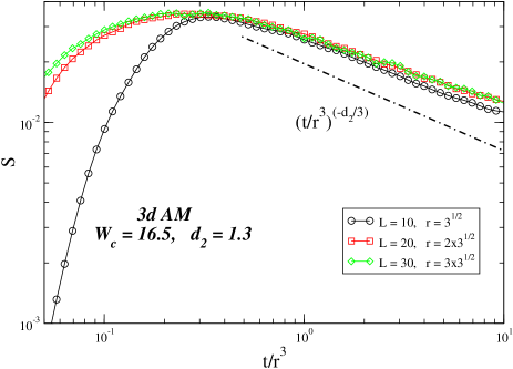
The application of the above results to the critical point of the Anderson localization transition is a subtle issue due to the absence of an exact solution to the Anderson localization problem and due to the limited sizes of 3D systems amendable to direct numerical diagonalization. Yet, it is rather well established that the multifractal behavior of the density correlation function, Eq. (8), is present at the Anderson transition point in 3D systems. In Fig. 9 we present the results of a direct numerical diagonalization of the 3D Anderson model at critical disorder $W=16.5$ and the nearest-neighbor hopping $V=1$. The density correlation function $\hat{\cal D}_{r,0}(t)$ is computed for three different values of $r$ and the corresponding three different system sizes such that $r/L\approx 0.17={\rm const}$. Thus geometrically the systems are “macroscopically similar” and the finite-size corrections of the type $r/L$, though appreciable, are the same for all the three cases. One can see that for $t>t_{max}$ ($\,t_{max}\,$ corresponds to the maximum of the scaling curve) all the three curves for $r^{3}\,\hat{\cal D}_{r,0}(t)$ collapse to the one single scaling curve $S(r^{3}/t)\sim(r^{3}/t)^{d_{2}}$ with rather good accuracy. In this region they exhibit the power-law behavior which is represented by Eq. (8), albeit with the power slightly modified by the finite-size $r/L$ effects.

The situation with the tail at $r^{3}\gg t$ is much worse. The curves for different $r$ diverge significantly as the scaling variable $t/r^{3}$ gets smaller. There is only one reason for such a behavior: it is the finite-size effects of the type $\ell_{0}/L_{t}$, where $\ell_{0}\sim(\rho_{0}V)^{-1/3}$ is the microscopic length which has been introduced in Ref.[KravCue, ], and $L_{t}^{3}=t/\rho_{0}$. Here $\rho_{0}\sim(a^{3}\,V\,W)^{-1}$ is the density of states, thus $\ell_{0}\sim a\,W^{1/3}$ is of the order of the lattice constant $a$. The parameter that controls the smallness of such finite-size effects is $(\ell_{0}/L_{t})^{3}\sim(tV)^{-1}=1/t$. Obviously, at small $t$ this parameter is no longer small and one cannot expect a scaling behavior in the region $t\ll 1$. On the other hand, $t_{max}\approx 0.3\,r^{3}$. So, it is only at large $r$ that one may observe a scaling behavior in a sufficiently wide interval $1\ll t<t_{max}$. We conclude that in order to meet the requirement $1\ll t<t_{max}$ and simultaneously to exclude the finite-size $r/L$ effects one should study really large 3D systems with $L\sim 100$ which is numerically a very hard problem.

In this situation we can only guess what is the form of the scaling function $S(r^{3}/t)$ at $t<t_{max}$ at the Anderson transition point of 3D systems. The most natural assumption is that it is exponentially small, and thus the Levy flights are absent, due to the short-range nature of the Anderson Hamiltonian. A counter-scenario in which the Levy flights may be present, is offered AKL by the observation of the ”explosion of high-gradient operators” in the non-linear supersymmetric sigma-model in $(2+\epsilon)$ dimensions. Unfortunately, this long-standing controversy still remains unresolved.