CERN-PH-TH/2012–134

RM3-TH/12-9

Higgs mass and vacuum stability
in the Standard Model at NNLO

Giuseppe Degrassia, Stefano Di Vitaa, Joan Elias-Mirób, José R. Espinosab,c,
Gian F. Giudiced, Gino Isidorid,e, Alessandro Strumiag,h
(a)𝑎(a) Dipartimento di Fisica, Università di Roma Tre and INFN Sez. Roma Tre, Roma, Italy
(b)𝑏(b) IFAE, Universitat Autónoma de Barcelona, 08193 Bellaterra, Barcelona, Spain
(c)𝑐(c) ICREA, Instituciò Catalana de Recerca i Estudis Avançats, Barcelona, Spain
(d)𝑑(d) CERN, Theory Division, CH–1211 Geneva 23, Switzerland
(e)𝑒(e) INFN, Laboratori Nazionali di Frascati, Via E. Fermi 40, Frascati, Italy
(g)𝑔(g) Dipartimento di Fisica, Università di Pisa and INFN Sez. Pisa, Pisa, Italy
(h)(h) National Institute of Chemical Physics and Biophysics, Tallinn, Estonia

Abstract

We present the first complete next-to-next-to-leading order analysis of the Standard Model Higgs potential. We computed the two-loop QCD and Yukawa corrections to the relation between the Higgs quartic coupling (λ𝜆\lambda) and the Higgs mass (Mhsubscript𝑀M_{h}), reducing the theoretical uncertainty in the determination of the critical value of Mhsubscript𝑀M_{h} for vacuum stability to 1 GeV. While λ𝜆\lambda at the Planck scale is remarkably close to zero, absolute stability of the Higgs potential is excluded at 98% C.L. for Mh<126GeVsubscript𝑀126GeVM_{h}<126\,\mathrm{GeV}. Possible consequences of the near vanishing of λ𝜆\lambda at the Planck scale, including speculations about the role of the Higgs field during inflation, are discussed.


1 Introduction

The value of the Higgs mass (Mhsubscript𝑀M_{h}) measured by present ATLAS and CMS data [1, 2], Mh=125.5±0.5GeVsubscript𝑀plus-or-minus125.50.5GeVM_{h}=125.5\pm 0.5\,\mathrm{GeV}, is intriguing: it is quite close to the minimum Mhsubscript𝑀M_{h} value that ensures absolute vacuum stability within the Standard Model (SM) which, in turn, implies a vanishing Higgs quartic coupling (λ𝜆\lambda) around the Planck scale. In order to assess if the measured Higgs mass is compatible with such a peculiar condition, a precise computation is needed.

The study of the stability of the SM vacuum has a long history [3, 4, 5] (see also [6, 7, 8] and references therein). The state-of-the-art analyses before the latest LHC data were done at the next-to-leading order (NLO) level [9, 10, 11, 12, 13, 14, 15, 16]. This is based on two-loop renormalization-group (RG) equations, one-loop threshold corrections at the electroweak scale (possibly improved with two-loop terms in the case of pure QCD corrections), and one-loop improved effective potential (see [17] for a numerically updated analysis).

With this paper all the ingredients necessary for a complete next-to-next-to-leading order (NNLO) analysis in the strong, top Yukawa and Higgs quartic couplings become available. In particular, complete three-loop beta functions for all the SM gauge couplings have been presented in [18], while the leading three-loop terms in the RG evolution of λ𝜆\lambda, the top Yukawa coupling (ytsubscript𝑦𝑡y_{t}) and the Higgs anomalous dimension have been computed in [19]. However, as pointed out in [17], the most important missing NNLO piece for the vacuum stability analysis are the two-loop threshold corrections to λ𝜆\lambda at the weak scale due to QCD and top Yukawa interactions, because such couplings are sizable at low energy. The calculation of such terms is presented in this work.

The relation that connects λ𝜆\lambda to the Higgs mass and to the the Fermi coupling (Gμsubscript𝐺𝜇G_{\mu}) can be written as

λ(μ)=GμMh22+Δλ(μ),𝜆𝜇subscript𝐺𝜇superscriptsubscript𝑀22Δ𝜆𝜇\lambda(\mu)=\frac{G_{\mu}M_{h}^{2}}{\sqrt{2}}+\Delta\lambda(\mu)~{}, (1)

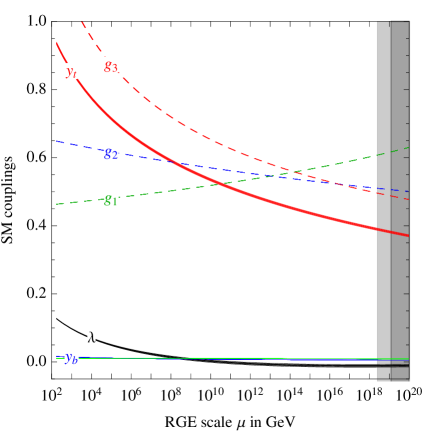
where Δλ(μ)Δ𝜆𝜇\Delta\lambda(\mu) denotes the sizable threshold corrections arising beyond the tree level. Given the rapid variation of λ𝜆\lambda around the weak scale (see fig. 1), these corrections play a significant role in determining the evolution of λ𝜆\lambda up to high energies. Computing Δλ(μ)Δ𝜆𝜇\Delta\lambda(\mu) at the one loop level, using two-loop beta functions for all the SM couplings, and varying the low-energy matching scale between Mt/2subscript𝑀𝑡2M_{t}/2 and 2Mt2subscript𝑀𝑡2M_{t}, leads to a ±2plus-or-minus2\pm 2 GeV error on Mhsubscript𝑀M_{h} [17]. The NNLO finite terms that we compute here allow us to reduce this error down to ±0.7GeVplus-or-minus0.7GeV\pm 0.7\,\mathrm{GeV}. While this work was in progress an independent calculation of the two-loop Yukawa-QCD contributions to Δλ(μ)Δ𝜆𝜇\Delta\lambda(\mu) has appeared [20]. Our result agrees with the one in ref. [20] for these contributions. However, our analysis includes also the two-loop terms coming from the Yukawa sector and can be considered the first complete NNLO evaluation of Δλ(μ)Δ𝜆𝜇\Delta\lambda(\mu). We stress that both these two-loop terms are needed to match the sizable two-loop scale dependence of λ𝜆\lambda around the weak scale, caused by the 32yt4gs2+30yt632superscriptsubscript𝑦𝑡4superscriptsubscript𝑔𝑠230superscriptsubscript𝑦𝑡6-32y_{t}^{4}g_{s}^{2}+30y_{t}^{6} terms in its beta function. As a result of this improved determination of Δλ(μ)Δ𝜆𝜇\Delta\lambda(\mu), we are able to obtain a significant reduction of the theoretical error on Mhsubscript𝑀M_{h} compared to previous works.

Refer to caption      Refer to caption
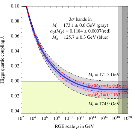
Figure 1: Left: SM RG evolution of the gauge couplings g1=5/3g,g2=g,g3=gsformulae-sequencesubscript𝑔153superscript𝑔formulae-sequencesubscript𝑔2𝑔subscript𝑔3subscript𝑔𝑠g_{1}=\sqrt{5/3}g^{\prime},~{}g_{2}=g,~{}g_{3}=g_{s}, of the top and bottom Yukawa couplings (yt,ybsubscript𝑦𝑡subscript𝑦𝑏y_{t},y_{b}), and of the Higgs quartic coupling λ𝜆\lambda. All couplings are defined in the MS¯¯MS\overline{\rm MS} scheme. The thickness indicates the ±1σplus-or-minus1𝜎\pm 1\sigma uncertainty. Right: RG evolution of λ𝜆\lambda varying Mtsubscript𝑀𝑡M_{t}, Mhsubscript𝑀M_{h} and αssubscript𝛼s\alpha_{\rm s} by ±3σplus-or-minus3𝜎\pm 3\sigma.

Putting all the NNLO ingredients together, we estimate an overall theory error on Mhsubscript𝑀M_{h} of ±1.0GeVplus-or-minus1.0GeV\pm 1.0\,\mathrm{GeV} (see section 3). Our final results for the condition of absolute stability up to the Planck scale is

Mh[GeV]>129.4+1.4(Mt[GeV]173.10.7)0.5(αs(MZ)0.11840.0007)±1.0th.subscript𝑀delimited-[]GeVplus-or-minus129.41.4subscript𝑀𝑡delimited-[]GeV173.10.70.5subscript𝛼𝑠subscript𝑀𝑍0.11840.0007subscript1.0thM_{h}~{}[{\rm GeV}]>129.4+1.4\left(\frac{M_{t}~{}[{\rm GeV}]-173.1}{0.7}\right)-0.5\left(\frac{\alpha_{s}(M_{Z})-0.1184}{0.0007}\right)\pm 1.0_{\rm th}\ . (2)

Combining in quadrature the theoretical uncertainty with the experimental errors on Mtsubscript𝑀𝑡M_{t} and αssubscript𝛼𝑠\alpha_{s} we get

Mh>129.4±1.8GeV.subscript𝑀plus-or-minus129.41.8GeVM_{h}>129.4\pm 1.8~{}\,\mathrm{GeV}. (3)

From this result we conclude that vacuum stability of the SM up to the Planck scale is excluded at 2σ2𝜎2\sigma (98% C.L. one sided) for Mh<126GeVsubscript𝑀126GeVM_{h}<126\,\mathrm{GeV}.

Although the central values of Higgs and top masses do not favor a scenario with a vanishing Higgs self coupling at the Planck scale (MPlsubscript𝑀PlM_{\rm Pl}) — a possibility originally proposed in ref. [21] and discussed more recently in ref. [11, 12, 22, 14, 23] — the smallness of λ𝜆\lambda around MPlsubscript𝑀PlM_{\rm Pl} is quite remarkable (see fig. 1). Motivated by this observation, we have explored in more detail the robustness of the predictions for Mhsubscript𝑀M_{h} and Mtsubscript𝑀𝑡M_{t} assuming special boundary conditions on λ𝜆\lambda and its beta function around MPlsubscript𝑀PlM_{\rm Pl}, as advocated in [22]. We have also critically examined scenarios where the Higgs field plays a role during inflation. This could happen because of a non-minimal coupling to gravity that flattens the SM potential close to MPlsubscript𝑀PlM_{\rm Pl} [14], provided λ(MPl)𝜆subscript𝑀Pl\lambda(M_{\rm Pl}) is positive. Alternatively, the Higgs field could have caused inflation while it was trapped in a second unstable minimum of the potential that appears near MPlsubscript𝑀PlM_{\rm Pl} if λ(MPl)𝜆subscript𝑀Pl\lambda(M_{\rm Pl}) is positive and very close to zero [12], provided some non-SM mechanism is introduced to exit inflation [24, 25]. Beside some technical problems, these frameworks could become viable only if Mhsubscript𝑀M_{h} satisfies the stability condition in eq. (2). We therefore conclude that both these possibilities are not favored by present data, unless Mtsubscript𝑀𝑡M_{t} is below about 172 GeV or new-physics threshold corrections at the high scale modify the shape of the SM potential.

The paper is organized as follows: in section 2 we present the calculation of the threshold correction Δλ(μ)Δ𝜆𝜇\Delta\lambda(\mu). The numerical results for the condition of vacuum stability and, more generally, for the structure of the SM Higgs potential up to very high field values are discussed in section 3. The implications of these results for Planck scale physics are discussed in section 4. The results are summarized in the conclusions. We include also an appendix in which a ready-to-use expression for the two-loop effective potential is presented.

2 The two-loop threshold correction to λ(μ)𝜆𝜇\lambda(\mu)

In this section we present our main new result, namely the calculation of the two-loop contribution to Δλ(μ)Δ𝜆𝜇\Delta\lambda(\mu). We first obtain the yt6superscriptsubscript𝑦𝑡6y_{t}^{6} and yt4gs2superscriptsubscript𝑦𝑡4superscriptsubscript𝑔𝑠2y_{t}^{4}g_{s}^{2} terms from the calculation of the Higgs mass via the effective potential. Then, we present the full result for the two-loop QCD and Yukawa contribution to Δλ(μ)Δ𝜆𝜇\Delta\lambda(\mu) in the SM with the electroweak gauge couplings switched off (the so-called gauge-less limit).

2.1 Two-loop corrected Higgs mass from the effective potential

We write the SM potential for the Higgs doublet H𝐻H in the usual way:

V=m2|H|2+λ|H|4H=(G+(v+h+iG0)/2),formulae-sequence𝑉superscript𝑚2superscript𝐻2𝜆superscript𝐻4𝐻matrixsuperscript𝐺𝑣𝑖superscript𝐺02\displaystyle V=-m^{2}|H|^{2}+\lambda|H|^{4}\qquad H=\begin{pmatrix}G^{+}\cr(v+h+iG^{0})/\sqrt{2}\end{pmatrix}\ , (4)

so that, up to negligible width effects, the pole Higgs mass Mhsubscript𝑀M_{h} is the solution of the pole equation

Mh2=m2+3λv2+Πhh(Mh2),superscriptsubscript𝑀2superscript𝑚23𝜆superscript𝑣2subscriptΠsuperscriptsubscript𝑀2M_{h}^{2}=-m^{2}+3\lambda v^{2}+\Pi_{hh}(M_{h}^{2})\ , (5)

where m2superscript𝑚2m^{2}, λ𝜆\lambda and v𝑣v are MS¯¯MS\overline{\rm MS} renormalized quantities and Πhh(p2)subscriptΠsuperscript𝑝2\Pi_{hh}(p^{2}) is the Higgs self-energy (two-point) function, with external four-momentum p𝑝p. We rewrite this equation as

Mh2superscriptsubscript𝑀2\displaystyle M_{h}^{2} =\displaystyle= [m2+3λv2+Πhh(0)]+[Πhh(Mh2)Πhh(0)]delimited-[]superscript𝑚23𝜆superscript𝑣2subscriptΠ0delimited-[]subscriptΠsuperscriptsubscript𝑀2subscriptΠ0\displaystyle\left[-m^{2}+3\lambda v^{2}+\Pi_{hh}(0)\right]+\left[\Pi_{hh}(M_{h}^{2})-\Pi_{hh}(0)\right] (6)
=\displaystyle= [Mh2]V+ΔΠhh(Mh2).subscriptdelimited-[]superscriptsubscript𝑀2𝑉ΔsubscriptΠsuperscriptsubscript𝑀2\displaystyle{\left[M_{h}^{2}\right]}_{V}+\Delta\Pi_{hh}(M_{h}^{2})\ .

This step is convenient because the last term (which is computationally challenging) only gives corrections suppressed by the small Higgs coupling, in view of the smallness of Mh2=2λv2superscriptsubscript𝑀22𝜆superscript𝑣2M_{h}^{2}=2\lambda v^{2} at tree level. The first dominant term can be expressed in term of derivatives of the effective potential, Veffsubscript𝑉effV_{\rm eff}. Writing the effective potential as a sum of the tree-level part V0subscript𝑉0V_{0} plus radiative corrections ΔVΔ𝑉\Delta V

Veff=m22h2+λ4h4+ΔV,subscript𝑉effsuperscript𝑚22superscript2𝜆4superscript4Δ𝑉V_{\rm eff}=-\frac{m^{2}}{2}h^{2}+\frac{\lambda}{4}h^{4}+\Delta V\ , (7)

one finds

[Mh2]V=2Veff(h)2|h=v,subscriptdelimited-[]superscriptsubscript𝑀2𝑉evaluated-atsuperscript2subscript𝑉effsuperscript2𝑣{\left[M_{h}^{2}\right]}_{V}=\left.\frac{\partial^{2}V_{\rm eff}}{(\partial h)^{2}}\right|_{h=v}\ , (8)

where v𝑣v is the hh vev at the minimum of the effective potential, determined by the minimization condition

Veffh|h=v=[m2h+λh3+ΔVh]h=v.evaluated-atsubscript𝑉eff𝑣subscriptdelimited-[]superscript𝑚2𝜆superscript3Δ𝑉𝑣\left.\frac{\partial V_{\rm eff}}{\partial h}\right|_{h=v}=\left[-m^{2}h+\lambda h^{3}+\frac{\partial\Delta V}{\partial h}\right]_{h=v}\ . (9)

As usual, it is convenient to consider m2superscript𝑚2m^{2} as a free parameter fixed in terms of v𝑣v by the above equation, arriving at

[Mh2]V=[2λv21hΔVh+2ΔV(h)2]h=v.subscriptdelimited-[]superscriptsubscript𝑀2𝑉subscriptdelimited-[]2𝜆superscript𝑣21Δ𝑉superscript2Δ𝑉superscript2𝑣{\left[M_{h}^{2}\right]}_{V}=\left[2\lambda v^{2}-\frac{1}{h}\frac{\partial\Delta V}{\partial h}+\frac{\partial^{2}\Delta V}{(\partial h)^{2}}\right]_{h=v}\ . (10)

Defining the operator 𝒟m2superscriptsubscript𝒟𝑚2{\cal D}_{m}^{2} as111Notice that the term in 𝒟m2superscriptsubscript𝒟𝑚2{\cal D}_{m}^{2} linear in field-derivatives automatically takes into account the cancellation of hh-tadpoles (or alternatively, the minimization condition to get the right v𝑣v).

𝒟m2=[1hh+2(h)2]h=v,superscriptsubscript𝒟𝑚2subscriptdelimited-[]1superscript2superscript2𝑣{\cal D}_{m}^{2}=\left[-\frac{1}{h}\frac{\partial}{\partial h}+\frac{\partial^{2}}{(\partial h)^{2}}\right]_{h=v}\ , (11)

and noting that 2λv2=𝒟m2V02𝜆superscript𝑣2superscriptsubscript𝒟𝑚2subscript𝑉02\lambda v^{2}={\cal D}_{m}^{2}V_{0}, we can simply write [Mh2]V=𝒟m2Veffsubscriptdelimited-[]superscriptsubscript𝑀2𝑉superscriptsubscript𝒟𝑚2subscript𝑉eff{\left[M_{h}^{2}\right]}_{V}={\cal D}_{m}^{2}V_{\rm eff}, obtaining the following form for the Higgs mass:

Mh2=𝒟m2Veff+ΔΠhh(Mh2).superscriptsubscript𝑀2superscriptsubscript𝒟𝑚2subscript𝑉effΔsubscriptΠsuperscriptsubscript𝑀2M_{h}^{2}={\cal D}_{m}^{2}V_{\rm eff}+\Delta\Pi_{hh}(M_{h}^{2})\ . (12)

It gives the Higgs mass squared as the sum of two terms. The first is the Higgs mass obtained from the potential; this is not the complete pole Higgs mass and must be corrected for nonzero external momentum effects, which are taken care of by the last term, ΔΠhh(Mh2)ΔsubscriptΠsuperscriptsubscript𝑀2\Delta\Pi_{hh}(M_{h}^{2}). It is a straightforward exercise to verify that this expression for pole mass is independent of the renormalization scale μ𝜇\mu. In particular, one can easily prove that

ddlnμ[Mh2]V𝑑𝑑𝜇subscriptdelimited-[]superscriptsubscript𝑀2𝑉\displaystyle\frac{d}{d\ln\mu}{\left[M_{h}^{2}\right]}_{V} =\displaystyle= 2γ[Mh2]V,2𝛾subscriptdelimited-[]superscriptsubscript𝑀2𝑉\displaystyle-2\gamma{\left[M_{h}^{2}\right]}_{V}\ , (13)
ddlnμΔΠhh(Mh2)𝑑𝑑𝜇ΔsubscriptΠsuperscriptsubscript𝑀2\displaystyle\frac{d}{d\ln\mu}\Delta\Pi_{hh}(M_{h}^{2}) =\displaystyle= 2γ[Mh2ΔΠhh(Mh2)],2𝛾delimited-[]superscriptsubscript𝑀2ΔsubscriptΠsuperscriptsubscript𝑀2\displaystyle 2\gamma\left[M_{h}^{2}-\Delta\Pi_{hh}(M_{h}^{2})\right]\ , (14)

where γ𝛾\gamma is the Higgs anomalous dimension, describing its wave-function renormalization, γdlnh/dlnμ𝛾𝑑𝑑𝜇\gamma\equiv d\ln h/d\ln\mu.

Using eq. (12) and the one-loop result for Veffsubscript𝑉effV_{\rm eff} in eq. (74) of the appendix one obtains the one-loop Higgs mass correction. The explicit one-loop result for the pole mass is

Mh2=2λv2+δ1Mh2,superscriptsubscript𝑀22𝜆superscript𝑣2subscript𝛿1superscriptsubscript𝑀2M_{h}^{2}=2\lambda v^{2}+\delta_{1}M_{h}^{2}\ , (15)

with

δ1Mh2subscript𝛿1superscriptsubscript𝑀2\displaystyle\delta_{1}M_{h}^{2} =\displaystyle= 1(4π)2{3yt2(4mt2Mh2)B0(mt,mt,Mh)+6λ2v2(3h6+π3)\displaystyle\frac{1}{(4\pi)^{2}}\left\{3y_{t}^{2}(4m_{t}^{2}-M_{h}^{2})B_{0}(m_{t},m_{t},M_{h})+6\lambda^{2}v^{2}(3\ell_{h}-6+\pi\sqrt{3})\right. (16)
v24(3g48λg2+16λ2)B0(mW,mW,Mh)superscript𝑣243superscript𝑔48𝜆superscript𝑔216superscript𝜆2subscript𝐵0subscript𝑚𝑊subscript𝑚𝑊subscript𝑀\displaystyle-\frac{v^{2}}{4}(3g^{4}-8\lambda g^{2}+16\lambda^{2})B_{0}(m_{W},m_{W},M_{h})
v28(3G48λG2+16λ2)B0(mZ,mZ,Mh)superscript𝑣283superscript𝐺48𝜆superscript𝐺216superscript𝜆2subscript𝐵0subscript𝑚𝑍subscript𝑚𝑍subscript𝑀\displaystyle-\frac{v^{2}}{8}(3G^{4}-8\lambda G^{2}+16\lambda^{2})B_{0}(m_{Z},m_{Z},M_{h})
+2mW2[g22λ(W1)]+mZ2[G22λ(Z1)]},\displaystyle+2m_{W}^{2}\left[g^{2}-2\lambda(\ell_{W}-1)\right]+m_{Z}^{2}\left[G^{2}-2\lambda(\ell_{Z}-1)\right]\left\}\frac{}{}\right.,

where G2=g2+g 2superscript𝐺2superscript𝑔2superscript𝑔2G^{2}=g^{2}+g^{\prime\,2}. All parameters on the right-hand side (including v𝑣v) are MS¯¯MS\overline{\rm MS} running parameters (with the exception of Mh2superscriptsubscript𝑀2M_{h}^{2}, which appears through the external momentum dependence of the Higgs self-energy). As eq. (74) was obtained in the Landau gauge, v𝑣v in eq. (16) represents the gauge and scale-dependent vacuum expectation value of the Higgs field as computed in the Landau gauge. Similarly the ΔΠhh(Mh2)ΔsubscriptΠsuperscriptsubscript𝑀2\Delta\Pi_{hh}(M_{h}^{2}) contribution in that equation is computed in the Landau gauge. In eq. (16)

B0(ma,mb,mc)01ln(1x)ma2+xmb2x(1x)mc2iϵμ2dx,subscript𝐵0subscript𝑚𝑎subscript𝑚𝑏subscript𝑚𝑐superscriptsubscript011𝑥superscriptsubscript𝑚𝑎2𝑥superscriptsubscript𝑚𝑏2𝑥1𝑥superscriptsubscript𝑚𝑐2𝑖italic-ϵsuperscript𝜇2𝑑𝑥B_{0}(m_{a},m_{b},m_{c})\equiv-\int_{0}^{1}\ln\frac{(1-x)m_{a}^{2}+xm_{b}^{2}-x(1-x)m_{c}^{2}-i\epsilon}{\mu^{2}}dx\ , (17)

and xln(mx2/μ2)subscript𝑥superscriptsubscript𝑚𝑥2superscript𝜇2\ell_{x}\equiv\ln(m_{x}^{2}/\mu^{2}), with mxsubscript𝑚𝑥m_{x} the running mass for particle x𝑥x (mtytv/2subscript𝑚𝑡subscript𝑦𝑡𝑣2m_{t}\equiv y_{t}v/\sqrt{2}). One can explicitly check, using the RGEs for these parameters, that this expression for Mh2superscriptsubscript𝑀2M_{h}^{2} is indeed scale-independent at one-loop order.

Neglecting gauge couplings and setting Mh2=2λv2superscriptsubscript𝑀22𝜆superscript𝑣2M_{h}^{2}=2\lambda v^{2} in the one-loop terms, one obtains the approximate expression

δ1Mh22yt2v2(4π)2[λ(2+3t)3yt2t].similar-to-or-equalssubscript𝛿1superscriptsubscript𝑀22superscriptsubscript𝑦𝑡2superscript𝑣2superscript4𝜋2delimited-[]𝜆23subscript𝑡3superscriptsubscript𝑦𝑡2subscript𝑡\delta_{1}M_{h}^{2}\simeq\frac{2y_{t}^{2}v^{2}}{(4\pi)^{2}}\left[\lambda(2+3\ell_{t})-3y_{t}^{2}\ell_{t}\right]\ . (18)

To compute eq. (12) at the two-loop level one can use the two-loop effective potential [26] to calculate [Mh2]Vsubscriptdelimited-[]superscriptsubscript𝑀2𝑉{\left[M_{h}^{2}\right]}_{V} and the general results for two-loop scalar self-energies in [27] (supplemented by the results on two-loop momentum integrals of [28]) to calculate ΔΠhh(Mh2)ΔsubscriptΠsuperscriptsubscript𝑀2\Delta\Pi_{hh}(M_{h}^{2}). If we only keep the leading two-loop corrections to Mh2superscriptsubscript𝑀2M_{h}^{2} proportional to yt6superscriptsubscript𝑦𝑡6y_{t}^{6}, yt4gs2superscriptsubscript𝑦𝑡4superscriptsubscript𝑔𝑠2y_{t}^{4}g_{s}^{2}, dropping all subleading terms that depend on the electroweak gauge couplings or λ𝜆\lambda, our task is simplified dramatically. First, in the two-loop effective potential we only have to consider the diagrams depicted in fig. 2. Their contribution can be extracted from the expressions for VYsubscript𝑉𝑌V_{Y} and VFVsubscript𝑉𝐹𝑉V_{FV} in the appendix.

Refer to caption
Figure 2: Two-loop vacuum diagrams that give the dominant contribution (depending only on gssubscript𝑔𝑠g_{s} and ytsubscript𝑦𝑡y_{t}) to the SM two-loop effective potential.

Second, in the two-loop term ΔΠhh(2)(Mh2)ΔsubscriptsuperscriptΠ2superscriptsubscript𝑀2\Delta\Pi^{(2)}_{hh}(M_{h}^{2}) we can substitute the tree-level value Mh2=2λv2superscriptsubscript𝑀22𝜆superscript𝑣2M_{h}^{2}=2\lambda v^{2}, so that

ΔΠhh(2)(Mh2)Πhh(2)(2λv2)Πhh(2)(0).similar-to-or-equalsΔsubscriptsuperscriptΠ2superscriptsubscript𝑀2subscriptsuperscriptΠ22𝜆superscript𝑣2subscriptsuperscriptΠ20\Delta\Pi^{(2)}_{hh}(M_{h}^{2})\simeq\Pi^{(2)}_{hh}(2\lambda v^{2})-\Pi^{(2)}_{hh}(0)\ . (19)

It is then clear that the two-loop contributions coming from that term are proportional to λ𝜆\lambda and are therefore subdominant. In this section we neglect ΔΠhh(2)(Mh2)ΔsubscriptsuperscriptΠ2superscriptsubscript𝑀2\Delta\Pi^{(2)}_{hh}(M_{h}^{2}) completely.

To find the expression for the Higgs mass at two-loop precision, we must also take into account that Mh2superscriptsubscript𝑀2M_{h}^{2} has to be evaluated with one-loop precision in the argument of the one-loop term ΔΠhh(1)(Mh2)ΔsubscriptsuperscriptΠ1superscriptsubscript𝑀2\Delta\Pi^{(1)}_{hh}(M_{h}^{2}). Putting together all these pieces, keeping only the yt6superscriptsubscript𝑦𝑡6y_{t}^{6} and yt4gs2superscriptsubscript𝑦𝑡4superscriptsubscript𝑔𝑠2y_{t}^{4}g_{s}^{2} terms, we arrive at the following two-loop correction to eq. (15):

δ2Mh2=yt2v2(4π)4[16gs2yt2(3t2+t)3yt4(9t23t+2+π23)].subscript𝛿2superscriptsubscript𝑀2superscriptsubscript𝑦𝑡2superscript𝑣2superscript4𝜋4delimited-[]16superscriptsubscript𝑔𝑠2superscriptsubscript𝑦𝑡23superscriptsubscript𝑡2subscript𝑡3superscriptsubscript𝑦𝑡49superscriptsubscript𝑡23subscript𝑡2superscript𝜋23\delta_{2}M_{h}^{2}=\frac{y_{t}^{2}v^{2}}{(4\pi)^{4}}\left[16g_{s}^{2}y_{t}^{2}(3\ell_{t}^{2}+\ell_{t})-3y_{t}^{4}\left(9\ell_{t}^{2}-3\ell_{t}+2+\frac{\pi^{2}}{3}\right)\right]\ . (20)

The expression for Mhsubscript𝑀M_{h} as a function of λ𝜆\lambda can be inverted to obtain λ(μ)𝜆𝜇\lambda(\mu) as a function of the pole Higgs mass Mhsubscript𝑀M_{h}. To express λ(μ)𝜆𝜇\lambda(\mu) in terms of physical quantities (i.e.  Gμsubscript𝐺𝜇G_{\mu} and the pole masses MZsubscript𝑀𝑍M_{Z}, MWsubscript𝑀𝑊M_{W}, and Mtsubscript𝑀𝑡M_{t}) the relations between physical and MS¯¯MS\overline{\rm MS} parameters are needed. At the level of accuracy we are working only the relation between the yt(μ)subscript𝑦𝑡𝜇y_{t}(\mu) and Mtsubscript𝑀𝑡M_{t} and the one between v(μ)𝑣𝜇v(\mu) and Gμsubscript𝐺𝜇G_{\mu} are required. They are given by:

yt2(μ)superscriptsubscript𝑦𝑡2𝜇\displaystyle y_{t}^{2}(\mu) =\displaystyle= 22GμMt2[1+831(4π)2gs2(3LT4)+1(4π)22GμMt2(9LT+11)],22subscript𝐺𝜇superscriptsubscript𝑀𝑡2delimited-[]1831superscript4𝜋2superscriptsubscript𝑔𝑠23subscript𝐿𝑇41superscript4𝜋22subscript𝐺𝜇superscriptsubscript𝑀𝑡29subscript𝐿𝑇11\displaystyle 2\sqrt{2}G_{\mu}M_{t}^{2}\left[1+\frac{8}{3}\frac{1}{(4\pi)^{2}}g_{s}^{2}(3L_{T}-4)+\frac{1}{(4\pi)^{2}}\sqrt{2}G_{\mu}M_{t}^{2}(-9L_{T}+11)\right], (21)
v2(μ)superscript𝑣2𝜇\displaystyle v^{2}(\mu) =\displaystyle= 12Gμ+1(4π)2[3Mt2(2LT1)+MW2(56LW)+12MZ2(56LZ)\displaystyle\frac{1}{\sqrt{2}G_{\mu}}+\left.\frac{1}{(4\pi)^{2}}\right[3M_{t}^{2}(2L_{T}-1)+M_{W}^{2}(5-6L_{W})+\frac{1}{2}M_{Z}^{2}(5-6L_{Z}) (22)
+3MZ2MW24(MZ2MW2)(LZLW)12Mh23MW2Mh2MW2Mh2(LWLH)],\displaystyle\left.+\frac{3M_{Z}^{2}M_{W}^{2}}{4(M_{Z}^{2}-M_{W}^{2})}(L_{Z}-L_{W})-\frac{1}{2}M_{h}^{2}-\frac{3M_{W}^{2}M_{h}^{2}}{M_{W}^{2}-M_{h}^{2}}(L_{W}-L_{H})\right]\ ,

where LX=ln(Mx2/μ2)subscript𝐿𝑋superscriptsubscript𝑀𝑥2superscript𝜇2L_{X}=\ln(M_{x}^{2}/\mu^{2}), with masses in capital letters denoting pole masses.

We find:

λ(μ)=GμMh22+λ(1)(μ)+λ(2)(μ),𝜆𝜇subscript𝐺𝜇superscriptsubscript𝑀22superscript𝜆1𝜇superscript𝜆2𝜇\lambda(\mu)=\frac{G_{\mu}M_{h}^{2}}{\sqrt{2}}+\lambda^{(1)}(\mu)+\lambda^{(2)}(\mu)\ , (23)

with

λ(2)(μ)=λQCD,lead.(2)(μ)+λYuk,lead.(2)(μ)+,superscript𝜆2𝜇subscriptsuperscript𝜆2QCDlead𝜇subscriptsuperscript𝜆2Yuklead𝜇\lambda^{(2)}(\mu)=\lambda^{(2)}_{\rm QCD,lead.}(\mu)+\lambda^{(2)}_{\rm Yuk,lead.}(\mu)+\ldots\ , (24)

where the ellipsis stands for the subleading terms neglected in this section. The known one loop term is

λ(1)(μ)superscript𝜆1𝜇\displaystyle\lambda^{(1)}(\mu) =\displaystyle= 12Gμ21(4π)2{6(LHLW)Mh6Mh2MW28(2MW4+MZ4)2(3+6LT)Mh2Mt2\displaystyle\frac{1}{2}G_{\mu}^{2}\frac{1}{(4\pi)^{2}}\left\{\frac{6(L_{H}-L_{W})M_{h}^{6}}{M_{h}^{2}-M_{W}^{2}}-8\left(2M_{W}^{4}+M_{Z}^{4}\right)-2(-3+6L_{T})M_{h}^{2}M_{t}^{2}\right. (25)
+Mh4(1915LH+6LW33π)+12(Mh24Mt2)Mt2B0(Mt,Mt,Mh)superscriptsubscript𝑀41915subscript𝐿𝐻6subscript𝐿𝑊33𝜋12superscriptsubscript𝑀24superscriptsubscript𝑀𝑡2superscriptsubscript𝑀𝑡2subscript𝐵0subscript𝑀𝑡subscript𝑀𝑡subscript𝑀\displaystyle+M_{h}^{4}\left(19-15L_{H}+6L_{W}-3\sqrt{3}\pi\right)+12(M_{h}^{2}-4M_{t}^{2})M_{t}^{2}B_{0}(M_{t},M_{t},M_{h})
+2(Mh44Mh2MW2+12MW4)B0(MW,MW,Mh)2superscriptsubscript𝑀44superscriptsubscript𝑀2superscriptsubscript𝑀𝑊212superscriptsubscript𝑀𝑊4subscript𝐵0subscript𝑀𝑊subscript𝑀𝑊subscript𝑀\displaystyle+2\left(M_{h}^{4}-4M_{h}^{2}M_{W}^{2}+12M_{W}^{4}\right)B_{0}(M_{W},M_{W},M_{h})
+(Mh44Mh2MZ2+12MZ4)B0(MZ,MZ,Mh)superscriptsubscript𝑀44superscriptsubscript𝑀2superscriptsubscript𝑀𝑍212superscriptsubscript𝑀𝑍4subscript𝐵0subscript𝑀𝑍subscript𝑀𝑍subscript𝑀\displaystyle+\left(M_{h}^{4}-4M_{h}^{2}M_{Z}^{2}+12M_{Z}^{4}\right)B_{0}(M_{Z},M_{Z},M_{h})
+Mh2[2(8LW7)MW2+(8LZ7)MZ26MZ2MW2MZ2MW2(LZLW)]},\displaystyle\left.+M_{h}^{2}\left[2(8L_{W}-7)M_{W}^{2}+(8L_{Z}-7)M_{Z}^{2}-\frac{6M_{Z}^{2}M_{W}^{2}}{M_{Z}^{2}-M_{W}^{2}}(L_{Z}-L_{W})\right]\right\}\ ,

and the leading two loop QCD and Yukawa terms are

λQCD,lead.(2)(μ)subscriptsuperscript𝜆2QCDlead𝜇\displaystyle\lambda^{(2)}_{\rm QCD,lead.}(\mu) =\displaystyle= Gμ2Mt4(4π)464gs2(μ)(46LT+3LT2),superscriptsubscript𝐺𝜇2superscriptsubscript𝑀𝑡4superscript4𝜋464superscriptsubscript𝑔𝑠2𝜇46subscript𝐿𝑇3superscriptsubscript𝐿𝑇2\displaystyle\frac{G_{\mu}^{2}M_{t}^{4}}{(4\pi)^{4}}64g_{s}^{2}(\mu)\left(-4-6L_{T}+3L_{T}^{2}\right)\ , (26)
λYuk,lead.(2)(μ)subscriptsuperscript𝜆2Yuklead𝜇\displaystyle\lambda^{(2)}_{\rm Yuk,lead.}(\mu) =\displaystyle= 82Gμ3Mt6(4π)4(30+π2+36LT45LT2).82superscriptsubscript𝐺𝜇3superscriptsubscript𝑀𝑡6superscript4𝜋430superscript𝜋236subscript𝐿𝑇45superscriptsubscript𝐿𝑇2\displaystyle\frac{8\sqrt{2}G_{\mu}^{3}M_{t}^{6}}{(4\pi)^{4}}\left(30+\pi^{2}+36L_{T}-45L_{T}^{2}\right)\ . (27)

The above expression for λ(μ)𝜆𝜇\lambda(\mu) has the correct dependence on the renormalization scale μ𝜇\mu, so that both sides of (23) evolve with μ𝜇\mu in the same way to the order we work.

2.2 Two-loop contribution to Δλ(μ)Δ𝜆𝜇\Delta\lambda(\mu) in the gauge-less SM

In this section we go beyond the leading yt6superscriptsubscript𝑦𝑡6y_{t}^{6} and yt4gs2superscriptsubscript𝑦𝑡4superscriptsubscript𝑔𝑠2y_{t}^{4}g_{s}^{2} contributions to Δλ(μ)Δ𝜆𝜇\Delta\lambda(\mu) discussed in the previous section and derive the QCD and Yukawa corrections in the SM with the electroweak gauge couplings switched off. We first discuss the two-loop renormalization of the Higgs sector of the SM and then derive the 2-loop relation between λ(μ)𝜆𝜇\lambda(\mu) and the physical parameters Gμ,Mtsubscript𝐺𝜇subscript𝑀𝑡G_{\mu},M_{t}, and Mhsubscript𝑀M_{h}. In our derivation we follow closely ref.[29].

We start from the unrenormalized Higgs potential, eq. (4) written in terms of bare quantities, and set m2mr2δm2,λλrδλ,vvrδvformulae-sequencesuperscript𝑚2superscriptsubscript𝑚𝑟2𝛿superscript𝑚2formulae-sequence𝜆subscript𝜆𝑟𝛿𝜆𝑣subscript𝑣𝑟𝛿𝑣m^{2}\to m_{r}^{2}-\delta m^{2},\>\lambda\to\lambda_{r}-\delta\lambda,\>v\to v_{r}-\delta v. Then, assuming δm2,δλ,δv𝛿superscript𝑚2𝛿𝜆𝛿𝑣\delta m^{2},\>\delta\lambda,\>\delta v of 𝒪(α)𝒪𝛼{\cal O}(\alpha), we obtain

V=VrδV,𝑉subscript𝑉𝑟𝛿𝑉V=V_{r}-\delta V\ , (28)

where, putting mr2=λrvr2superscriptsubscript𝑚𝑟2subscript𝜆𝑟superscriptsubscript𝑣𝑟2m_{r}^{2}=\lambda_{r}v_{r}^{2},

Vrsubscript𝑉𝑟\displaystyle V_{r} =\displaystyle= λr[G+G(G+G+h2+G0)2+14(h2+G02)2]subscript𝜆𝑟delimited-[]superscript𝐺superscript𝐺superscriptsuperscript𝐺superscript𝐺superscript2subscript𝐺0214superscriptsuperscript2superscriptsubscript𝐺022\displaystyle\lambda_{r}\left[G^{+}G^{-}\left(G^{+}G^{-}+h^{2}+G_{0}\right)^{2}+\frac{1}{4}\left(h^{2}+G_{0}^{2}\right)^{2}\right] (29)
+λrvrh[h2+G02+2G+G]+12Mh2h2,subscript𝜆𝑟subscript𝑣𝑟delimited-[]superscript2superscriptsubscript𝐺022superscript𝐺superscript𝐺12superscriptsubscript𝑀2superscript2\displaystyle+\,\lambda_{r}v_{r}\,h\left[h^{2}+G_{0}^{2}+2\,G^{+}G^{-}\right]+\frac{1}{2}M_{h}^{2}\,h^{2}\ ,

with Mh=2λrvr2subscript𝑀2subscript𝜆𝑟superscriptsubscript𝑣𝑟2M_{h}=2\,\lambda_{r}v_{r}^{2}, while, up to two-loop terms,

δV𝛿𝑉\displaystyle\delta V =\displaystyle= δλ[G+G(G+G+h2+G0)2+14(h2+G02)2]𝛿𝜆delimited-[]superscript𝐺superscript𝐺superscriptsuperscript𝐺superscript𝐺superscript2subscript𝐺0214superscriptsuperscript2superscriptsubscript𝐺022\displaystyle\delta\lambda\left[G^{+}G^{-}\left(G^{+}G^{-}+h^{2}+G_{0}\right)^{2}+\frac{1}{4}\left(h^{2}+G_{0}^{2}\right)^{2}\right] (30)
+[λr(δv22vr+(δv2)28vr3)+vrδλ(1δv22vr2)]h[h2+G02+2G+G]delimited-[]subscript𝜆𝑟𝛿superscript𝑣22subscript𝑣𝑟superscript𝛿superscript𝑣228superscriptsubscript𝑣𝑟3subscript𝑣𝑟𝛿𝜆1𝛿superscript𝑣22superscriptsubscript𝑣𝑟2delimited-[]superscript2superscriptsubscript𝐺022superscript𝐺superscript𝐺\displaystyle+\left[\lambda_{r}\left(\frac{\delta v^{2}}{2\,v_{r}}+\frac{(\delta v^{2})^{2}}{8\,v_{r}^{3}}\right)+v_{r}\,\delta\lambda\left(1-\frac{\delta v^{2}}{2\,v_{r}^{2}}\right)\right]h\left[h^{2}+G_{0}^{2}+2\,G^{+}G^{-}\right]
+δτ(12G02+G+G)+12δMh2h2+vrδτ(1δv22vr2)h.𝛿𝜏12superscriptsubscript𝐺02superscript𝐺superscript𝐺12𝛿superscriptsubscript𝑀2superscript2subscript𝑣𝑟𝛿𝜏1𝛿superscript𝑣22superscriptsubscript𝑣𝑟2\displaystyle+\delta\tau\left(\frac{1}{2}G_{0}^{2}+G^{+}G^{-}\right)+\frac{1}{2}\delta M_{h}^{2}h^{2}+v_{r}\,\delta\tau\left(1-\frac{\delta v^{2}}{2\,v_{r}^{2}}\right)\,h~{}.

In eq. (30)

δMh2𝛿superscriptsubscript𝑀2\displaystyle\delta M_{h}^{2} =\displaystyle= 3[λrδv2+vr2δλ(1δv2vr2)]δm2,3delimited-[]subscript𝜆𝑟𝛿superscript𝑣2superscriptsubscript𝑣𝑟2𝛿𝜆1𝛿superscript𝑣2superscriptsubscript𝑣𝑟2𝛿superscript𝑚2\displaystyle 3\left[\lambda_{r}\delta v^{2}+v_{r}^{2}\delta\lambda\left(1-\frac{\delta v^{2}}{v_{r}^{2}}\right)\right]-\delta m^{2}\ , (31)
δτ𝛿𝜏\displaystyle\delta\tau =\displaystyle= λrδv2+vr2δλ(1δv2vr2)δm2,subscript𝜆𝑟𝛿superscript𝑣2superscriptsubscript𝑣𝑟2𝛿𝜆1𝛿superscript𝑣2superscriptsubscript𝑣𝑟2𝛿superscript𝑚2\displaystyle\lambda_{r}\delta v^{2}+v_{r}^{2}\delta\lambda\left(1-\frac{\delta v^{2}}{v_{r}^{2}}\right)-\delta m^{2}\ , (32)

and δv2𝛿superscript𝑣2\delta v^{2} is related to δv𝛿𝑣\delta v through vr2δv2=vrδvsuperscriptsubscript𝑣𝑟2𝛿superscript𝑣2subscript𝑣𝑟𝛿𝑣\sqrt{v_{r}^{2}-\delta v^{2}}=v_{r}-\delta v.

Following ref.[29] we require the cancellation of the tadpole contribution by setting

δτ(1δv22vr2)=Tvr,𝛿𝜏1𝛿superscript𝑣22superscriptsubscript𝑣𝑟2𝑇subscript𝑣𝑟\delta\tau\left(1-\frac{\delta v^{2}}{2\,v_{r}^{2}}\right)=-\frac{T}{v_{r}}\ , (33)

where iT𝑖𝑇iT is the sum of the tadpole diagrams with the external leg extracted. We identify Mh2superscriptsubscript𝑀2M_{h}^{2} in Vrsubscript𝑉𝑟V_{r} with the on-shell Higgs mass leading to the condition

δMh2=ReΠhh(Mh2),𝛿superscriptsubscript𝑀2ResubscriptΠsuperscriptsubscript𝑀2\delta M_{h}^{2}={\rm Re}\,\Pi_{hh}(M_{h}^{2})\ , (34)

where the Πhh(Mh2)subscriptΠsuperscriptsubscript𝑀2\Pi_{hh}(M_{h}^{2}) in the above equation includes only the contribution of the self-energy diagrams because eq. (33) is enforced. A third condition can be obtained by looking directly at the muon-decay process. At the two-loop level we can write

Gμ2=12v02{1AWWMW02+VW+MW02BW+(AWWMW2)2AWWVWMW2},subscript𝐺𝜇212superscriptsubscript𝑣021subscript𝐴𝑊𝑊superscriptsubscript𝑀subscript𝑊02subscript𝑉𝑊superscriptsubscript𝑀subscript𝑊02subscript𝐵𝑊superscriptsubscript𝐴𝑊𝑊superscriptsubscript𝑀𝑊22subscript𝐴𝑊𝑊subscript𝑉𝑊superscriptsubscript𝑀𝑊2\frac{G_{\mu}}{\sqrt{2}}=\frac{1}{2v_{0}^{2}}\left\{1-\frac{A_{WW}}{M_{W_{0}}^{2}}+V_{W}+M_{W_{0}}^{2}B_{W}+\left(\frac{A_{WW}}{M_{W}^{2}}\right)^{2}-\frac{A_{WW}V_{W}}{M_{W}^{2}}\right\}\ , (35)

where v0subscript𝑣0v_{0} is the unrenormalized vacuum, AWWAWW(0)subscript𝐴𝑊𝑊subscript𝐴𝑊𝑊0A_{WW}\equiv A_{WW}(0) is the W𝑊W self-energy evaluated at zero external momenta, VWsubscript𝑉𝑊V_{W} and BWsubscript𝐵𝑊B_{W} are the relevant vertex and box contributions in the μ𝜇\mu-decay process and MW0subscript𝑀subscript𝑊0M_{W_{0}} is the unrenormalized W𝑊W mass. Performing the shifts v02vr2δv2superscriptsubscript𝑣02superscriptsubscript𝑣𝑟2𝛿superscript𝑣2v_{0}^{2}\to v_{r}^{2}-\delta v^{2}, MW0MW2δMW2subscript𝑀subscript𝑊0subscriptsuperscript𝑀2𝑊𝛿subscriptsuperscript𝑀2𝑊M_{W_{0}}\to M^{2}_{W}-\delta M^{2}_{W}, where δMW2=ReAWW(MW2)𝛿subscriptsuperscript𝑀2𝑊Resubscript𝐴𝑊𝑊superscriptsubscript𝑀𝑊2\delta M^{2}_{W}={\rm Re}A_{WW}(M_{W}^{2}), and working at the two-loop level we arrive at

vr2=12Gμ12Gμ{AWWMW2E+AWWδMW2MW4(AWWMW2)2+AWWVWMW2+δMW2BW}+δv2,superscriptsubscript𝑣𝑟212subscript𝐺𝜇12subscript𝐺𝜇subscript𝐴𝑊𝑊superscriptsubscript𝑀𝑊2𝐸subscript𝐴𝑊𝑊𝛿superscriptsubscript𝑀𝑊2superscriptsubscript𝑀𝑊4superscriptsubscript𝐴𝑊𝑊superscriptsubscript𝑀𝑊22subscript𝐴𝑊𝑊subscript𝑉𝑊superscriptsubscript𝑀𝑊2𝛿superscriptsubscript𝑀𝑊2subscript𝐵𝑊𝛿superscript𝑣2v_{r}^{2}=\frac{1}{\sqrt{2}\,G_{\mu}}-\frac{1}{\sqrt{2}\,G_{\mu}}\left\{\frac{A_{WW}}{M_{W}^{2}}-E+\frac{A_{WW}\,\delta M_{W}^{2}}{M_{W}^{4}}-\left(\frac{A_{WW}}{M_{W}^{2}}\right)^{2}+\frac{A_{WW}V_{W}}{M_{W}^{2}}+\delta M_{W}^{2}B_{W}\right\}+\delta v^{2}\ , (36)

where EVW+MW2BW𝐸subscript𝑉𝑊superscriptsubscript𝑀𝑊2subscript𝐵𝑊E\equiv V_{W}+M_{W}^{2}B_{W}. We identify the renormalized vacuum by vr2=1/(2Gμ)superscriptsubscript𝑣𝑟212subscript𝐺𝜇v_{r}^{2}=1/(\sqrt{2}\,G_{\mu}), then δv2𝛿superscript𝑣2\delta v^{2} is defined to cancel the contribution of the curly bracket in eq. (36).

Our choice of renormalization conditions implies that the renormalized quartic Higgs coupling is set equal to

λr=Gμ2Mh2,subscript𝜆𝑟subscript𝐺𝜇2superscriptsubscript𝑀2\lambda_{r}=\frac{G_{\mu}}{\sqrt{2}}M_{h}^{2}\ , (37)

while eqs.(3136) can be used to obtain the correction δλ𝛿𝜆\delta\lambda. Writing

δλ=δλ(1)+δλ(2),𝛿𝜆𝛿superscript𝜆1𝛿superscript𝜆2\delta\lambda=\delta\lambda^{(1)}+\delta\lambda^{(2)}~{}, (38)

where the superscript indicates the loop order, we have

δλ(1)𝛿superscript𝜆1\displaystyle\delta\lambda^{(1)} =\displaystyle= Gμ2Mh2{AWW(1)MW2E(1)1Mh2[ReΠhh(1)(Mh2)+T(1)vr]}subscript𝐺𝜇2superscriptsubscript𝑀2superscriptsubscript𝐴𝑊𝑊1superscriptsubscript𝑀𝑊2superscript𝐸11superscriptsubscript𝑀2delimited-[]ResuperscriptsubscriptΠ1superscriptsubscript𝑀2superscript𝑇1subscript𝑣𝑟\displaystyle-\frac{G_{\mu}}{\sqrt{2}}M_{h}^{2}\left\{\frac{A_{WW}^{(1)}}{M_{W}^{2}}-E^{(1)}-\frac{1}{M_{h}^{2}}\left[{\rm Re}\,\Pi_{hh}^{(1)}(M_{h}^{2})+\frac{T^{(1)}}{v_{r}}\right]\right\} (39)
δλ(2)𝛿superscript𝜆2\displaystyle\delta\lambda^{(2)} =\displaystyle= Gμ2Mh2{AWW(2)MW2E(2)1Mh2[ReΠhh(2)(Mh2)+T(2)vr]\displaystyle-\frac{G_{\mu}}{\sqrt{2}}M_{h}^{2}\left\{\frac{A_{WW}^{(2)}}{M_{W}^{2}}-E^{(2)}-\frac{1}{M_{h}^{2}}\left[{\rm Re}\,\Pi_{hh}^{(2)}(M_{h}^{2})+\frac{T^{(2)}}{v_{r}}\right]\right. (40)
+\displaystyle+ (AWW(1)MW2E(1))(AWW(1)MW2E(1)1Mh2[ReΠhh(1)(Mh2)+32T(1)vr])superscriptsubscript𝐴𝑊𝑊1superscriptsubscript𝑀𝑊2superscript𝐸1superscriptsubscript𝐴𝑊𝑊1superscriptsubscript𝑀𝑊2superscript𝐸11superscriptsubscript𝑀2delimited-[]ResuperscriptsubscriptΠ1superscriptsubscript𝑀232superscript𝑇1subscript𝑣𝑟\displaystyle\left(\frac{A_{WW}^{(1)}}{M_{W}^{2}}-E^{(1)}\right)\left(\frac{A_{WW}^{(1)}}{M_{W}^{2}}-E^{(1)}-\frac{1}{M_{h}^{2}}\left[{\rm Re}\,\Pi_{hh}^{(1)}(M_{h}^{2})+\frac{3}{2}\frac{T^{(1)}}{v_{r}}\right]\right)
+\displaystyle+ AWW(1)δ(1)MW2MW4(AWW(1)MW2)2+AWW(1)VW(1)MW2+δ(1)MW2BW(1)}.\displaystyle\left.\frac{A_{WW}^{(1)}\,\delta^{(1)}M_{W}^{2}}{M_{W}^{4}}-\left(\frac{A_{WW}^{(1)}}{M_{W}^{2}}\right)^{2}+\frac{A_{WW}^{(1)}V^{(1)}_{W}}{M_{W}^{2}}+\delta^{(1)}M_{W}^{2}B_{W}^{(1)}\right\}~{}.

The connection between λrsubscript𝜆𝑟\lambda_{r}, as defined in eq. (37), and λ(μ)𝜆𝜇\lambda(\mu) can be easily derived using

λrδλ=λ(μ)δλ^,subscript𝜆𝑟𝛿𝜆𝜆𝜇𝛿^𝜆\lambda_{r}-\delta\lambda=\lambda(\mu)-\delta\hat{\lambda}\ , (41)

or

λ(μ)=Gμ2Mh2δλ+δλ^.𝜆𝜇subscript𝐺𝜇2superscriptsubscript𝑀2𝛿𝜆𝛿^𝜆\lambda(\mu)=\frac{G_{\mu}}{\sqrt{2}}M_{h}^{2}-\delta\lambda+\delta\hat{\lambda}~{}. (42)

In eqs. (41)–(42) δλ^𝛿^𝜆\delta\hat{\lambda} is the counterterm associated to λ(μ)𝜆𝜇\lambda(\mu), i.e. the counterterm that subtracts only the terms proportional to powers of 1/ϵ1italic-ϵ1/\epsilon and γln(4π)𝛾4𝜋\gamma-\ln(4\pi) in dimensional regularization, with d=42ϵ𝑑42italic-ϵd=4-2\,\epsilon being the dimension of space-time. Concerning the structure of the 1/ϵ1italic-ϵ1/\epsilon poles in δλ𝛿𝜆\delta\lambda and δλ^𝛿^𝜆\delta\hat{\lambda}, one notices that it should be identical once the poles in δλ𝛿𝜆\delta\lambda are expressed in terms of MS¯¯MS\overline{\rm MS} quantities. Then, after this operation is performed, a finite λ(μ)𝜆𝜇\lambda(\mu) is obtained.

Specializing the above discussion to the two-loop case we have

λ(μ)=Gμ2Mh2δλ(1)|finδλ(2)|fin+Δ𝜆𝜇subscript𝐺𝜇2superscriptsubscript𝑀2evaluated-at𝛿superscript𝜆1finevaluated-at𝛿superscript𝜆2finΔ\lambda(\mu)=\frac{G_{\mu}}{\sqrt{2}}M_{h}^{2}-\delta\lambda^{(1)}|_{\rm fin}-\delta\lambda^{(2)}|_{\rm fin}+\Delta (43)

from which we identify the one- and two-loop contributions entering eq. (23),

λ(1)(μ)superscript𝜆1𝜇\displaystyle\lambda^{(1)}(\mu) =\displaystyle= δλ(1)|fin,evaluated-at𝛿superscript𝜆1fin\displaystyle-\delta\lambda^{(1)}|_{\rm fin}~{}, (44)
which reproduces the one-loop result of ref.[29] and
λ(2)(μ)superscript𝜆2𝜇\displaystyle\lambda^{(2)}(\mu) =\displaystyle= δλ(2)|fin+Δ.evaluated-at𝛿superscript𝜆2finΔ\displaystyle-\delta\lambda^{(2)}|_{\rm fin}+\Delta~{}. (45)

In eqs. (43)–(45) the subscript ‘fin’ denotes the finite part of the quantity involved and ΔΔ\Delta is the two-loop finite contribution that is obtained when the OS parameters entering the 1/ϵitalic-ϵ\epsilon pole in δλ(1)𝛿superscript𝜆1\delta\lambda^{(1)} are expressed in terms of MS¯¯MS\overline{\rm MS} quantities, the finite contribution coming from the O(ϵ)𝑂italic-ϵO(\epsilon) part of the shifts.

Differentiating eq. (43) with respect to μ𝜇\mu, the known two-loop beta function for the Higgs quartic coupling is recovered. It should be recalled that the right-hand side of eq. (43) is expressed in terms of physical quantities, then the dependence on μ𝜇\mu in that equation is explicit. To obtain the correct two-loop beta function, one has first to differentiate with respect to μ𝜇\mu and then to express the one-loop part in terms of MS¯¯MS\overline{\rm MS} quantities.

The computation of λ(2)(μ)superscript𝜆2𝜇\lambda^{(2)}(\mu) in the full SM is quite cumbersome, see eq. (40). However, the calculation can be greatly simplified if one considers the gauge-less limit of the SM in which the electroweak interactions are neglected, i.e. the gauge couplings g𝑔g and gsuperscript𝑔g^{\prime} are set equal to zero. In this limit, eq. (40) simplifies to

(δλ(2)Δ)g.l.subscript𝛿superscript𝜆2Δformulae-sequence𝑔𝑙\displaystyle\left(\delta\lambda^{(2)}-\Delta\right)_{g.l.} =\displaystyle= Gμ2Mh2{AWW(2)MW21Mh2[ReΠhh(2)(Mh2)+T(2)vr]\displaystyle-\frac{G_{\mu}}{\sqrt{2}}M_{h}^{2}\left\{\frac{A_{WW}^{(2)}}{M_{W}^{2}}-\frac{1}{M_{h}^{2}}\left[{\rm Re}\,\Pi_{hh}^{(2)}(M_{h}^{2})+\frac{T^{(2)}}{v_{r}}\right]\right. (46)
+\displaystyle+ AWW(1)MW2(AWW(1)MW21Mh2[ReΠhh(1)(Mh2)+32T(1)vr])}g.l.Δg.l.,\displaystyle\left.\frac{A_{WW}^{(1)}}{M_{W}^{2}}\left(\frac{A_{WW}^{(1)}}{M_{W}^{2}}-\frac{1}{M_{h}^{2}}\left[{\rm Re}\,\Pi_{hh}^{(1)}(M_{h}^{2})+\frac{3}{2}\frac{T^{(1)}}{v_{r}}\right]\right)\right\}_{g.l.}-\Delta_{g.l.}\ ,

where the subscript g.l.formulae-sequence𝑔𝑙g.l. means that we have considered in the various self-energies only diagrams involving the top and bottom quarks, the Higgs and the Goldstone bosons, the latter with vanishing mass, and the limit g,g0𝑔superscript𝑔0g,g^{\prime}\to 0 is taken.

Using eq. (46) we compute the QCD and the Yukawa contribution to λ(2)(μ)superscript𝜆2𝜇\lambda^{(2)}(\mu). The top Yukawa-QCD contribution, λQCD(2)(μ)subscriptsuperscript𝜆2QCD𝜇\lambda^{(2)}_{\rm QCD}(\mu), is obtained evaluating the relevant diagrams via a Taylor series in xhtMh2/Mt2subscript𝑥𝑡superscriptsubscript𝑀2superscriptsubscript𝑀𝑡2x_{ht}\equiv M_{h}^{2}/M_{t}^{2} up to fourth order

λQCD(2)(μ)subscriptsuperscript𝜆2QCD𝜇\displaystyle\lambda^{(2)}_{\rm QCD}(\mu) =\displaystyle= Gμ2Mt4(4π)4NcCFgs2(μ)[16(46LT+3LT2)\displaystyle\frac{G_{\mu}^{2}M_{t}^{4}}{(4\pi)^{4}}\,N_{c}\,C_{F}\,g_{s}^{2}(\mu)\bigg{[}16\left(-4-6L_{T}+3L_{T}^{2}\right) (47)
+\displaystyle+ xht(352π23+12LT12LT2)+xht261135+xht312236300+xht4431231323000],\displaystyle\left.x_{ht}\left(35-\frac{2\,\pi^{2}}{3}+12L_{T}-12L_{T}^{2}\right)+x_{ht}^{2}\frac{61}{135}+x_{ht}^{3}\frac{1223}{6300}+x_{ht}^{4}\frac{43123}{1323000}\right]\ ,

where Ncsubscript𝑁𝑐N_{c} and CFsubscript𝐶𝐹C_{F} are color factors (Nc=3,CF=4/3formulae-sequencesubscript𝑁𝑐3subscript𝐶𝐹43N_{c}=3,\,C_{F}=4/3). Equation (47) shows that the series converges very fast. Our result is in agreement with ref.[20], the numerical difference between eq. (47) and the expression of ref.[20] for Mh125similar-tosubscript𝑀125M_{h}\sim 125 GeV being negligible.

The Yukawa contribution, λYuk(2)(μ)subscriptsuperscript𝜆2Yuk𝜇\lambda^{(2)}_{\rm Yuk}(\mu), is (neglecting the small bottom Yukawa)

λYuk(2)(μ)subscriptsuperscript𝜆2Yuk𝜇\displaystyle\lambda^{(2)}_{\rm Yuk}(\mu) =\displaystyle= 2Gμ3Mt6(4π)4{Nc2[16B0(Mt,Mt,Mh)(1+2LT)\displaystyle\frac{\sqrt{2}G_{\mu}^{3}M_{t}^{6}}{(4\pi)^{4}}\Bigg{\{}N_{c}^{2}\Bigg{[}16B_{0}(M_{t},M_{t},M_{h})(-1+2L_{T}) (48)
+xht((1+4B0(Mt,Mt,Mh)2LT)(12LT))]\displaystyle~{}~{}~{}~{}~{}~{}~{}~{}~{}~{}~{}~{}~{}~{}~{}~{}+x_{ht}\left((1+4B_{0}(M_{t},M_{t},M_{h})-2L_{T})(1-2L_{T})\right)\Bigg{]}
+Nc[16+83π2+32B0(Mt,Mh,Mt)(1+2LT)48LT+40LT2\displaystyle+N_{c}\left[16+\frac{8}{3}\pi^{2}+32B_{0}(M_{t},M_{h},M_{t})(1+2L_{T})-48L_{T}+40L_{T}^{2}\right.
xht(9296+163π2+48B0(Mh,Mh,Mh)16LH(1LT)\displaystyle~{}~{}~{}~{}~{}~{}~{}~{}~{}-x_{ht}\left(\frac{929}{6}+\frac{16}{3}\pi^{2}+48B_{0}(M_{h},M_{h},M_{h})-16L_{H}\left(1-L_{T}\right)\right.
+B0(Mt,Mh,Mt)(763+32LT)+1903LT+58LT2)\displaystyle~{}~{}~{}~{}~{}~{}~{}~{}~{}~{}~{}~{}~{}~{}~{}\left.+B_{0}(M_{t},M_{h},M_{t})\left(\frac{76}{3}+32L_{T}\right)+\frac{190}{3}L_{T}+58L_{T}^{2}\right)
+xht2(17629270+83π223LH+B0(Mh,Mh,Mh)(2718LT)+40LT\displaystyle~{}~{}~{}~{}~{}~{}~{}~{}~{}+x_{ht}^{2}\left(\frac{17629}{270}+\frac{8}{3}\pi^{2}-\frac{2}{3}L_{H}+B_{0}(M_{h},M_{h},M_{h})\left(27-18L_{T}\right)+40L_{T}\right.
+10LTLH+12LT2+B0(Mt,Mh,Mt)(133+4LT))\displaystyle~{}~{}~{}~{}~{}~{}~{}~{}~{}~{}~{}~{}~{}~{}~{}\left.+10L_{T}L_{H}+12L_{T}^{2}+B_{0}(M_{t},M_{h},M_{t})\left(\frac{13}{3}+4L_{T}\right)\right)
+xht3(1181900π22+6130B0(Mh,Mh,Mh)+5990LH\displaystyle~{}~{}~{}~{}~{}~{}~{}~{}~{}+x_{ht}^{3}\left(\frac{1181}{900}-\frac{\pi^{2}}{2}+\frac{61}{30}B_{0}(M_{h},M_{h},M_{h})+\frac{59}{90}L_{H}\right.
235B0(Mt,Mh,Mt)6863LT)]\displaystyle~{}~{}~{}~{}~{}~{}~{}~{}~{}~{}~{}~{}~{}~{}~{}\left.\left.-\frac{2}{35}B_{0}(M_{t},M_{h},M_{t})-\frac{68}{63}L_{T}\right)\right]
+xht3[1316π2+(729213543π)S2111LH+36LH2\displaystyle+x_{ht}^{3}\left[\frac{131}{6}\pi^{2}+\left(\frac{729}{2}-\frac{135}{4}\sqrt{3}\,\pi\right)S_{2}-111L_{H}+36L_{H}^{2}\right.
+π(22534+183LH)+75+72ζ34]},\displaystyle~{}~{}~{}~{}~{}~{}~{}~{}~{}~{}~{}~{}~{}\left.\left.+\pi\left(\frac{-225\sqrt{3}}{4}+18\sqrt{3}L_{H}\right)+\frac{75+72\,\zeta_{3}}{4}\right]\right\}\ ,

where B0(Mh,Mh,Mh)=2LHπ/3subscript𝐵0subscript𝑀subscript𝑀subscript𝑀2subscript𝐿𝐻𝜋3B_{0}(M_{h},M_{h},M_{h})=2-L_{H}-\pi/\sqrt{3} and S2=4/(93)Cl2(π/3)=0.260434138subscript𝑆2493subscriptCl2𝜋30.260434138S_{2}=4/(9\,\sqrt{3})\,{\rm Cl}_{2}(\pi/3)=0.260434138\ldots In eq. (48) the terms proportional to Nc2superscriptsubscript𝑁𝑐2N_{c}^{2} and Nc0superscriptsubscript𝑁𝑐0N_{c}^{0} were computed exactly while the ones proportional to Ncsubscript𝑁𝑐N_{c} were computed via an asymptotic expansion in the large top mass up to xht3superscriptsubscript𝑥𝑡3x_{ht}^{3} terms exploiting the asymptotic-expansion techniques developed in ref.[30]. The part independent of Ncsubscript𝑁𝑐N_{c} in eq. (48) was computed using the results for the two-loop on-shell master integrals of ref.[31].

We end this section by commenting on the size of the terms suppressed by powers of xhtsubscript𝑥𝑡x_{ht} with respect to the yt4gs2superscriptsubscript𝑦𝑡4superscriptsubscript𝑔𝑠2y_{t}^{4}g_{s}^{2} and yt6superscriptsubscript𝑦𝑡6y_{t}^{6} contribution in eqs. (47, 48). While in the QCD case, eq. (47), the xhtsubscript𝑥𝑡x_{ht} suppressed terms are indeed smaller than the yt4gs2superscriptsubscript𝑦𝑡4superscriptsubscript𝑔𝑠2y_{t}^{4}g_{s}^{2} contribution, the same is not true in the Yukawa case, eq. (48), where the xhtsubscript𝑥𝑡x_{ht} terms are actually larger than the yt6superscriptsubscript𝑦𝑡6y_{t}^{6} contribution.

3 Extrapolating the SM up to the Planck scale

A full NNLO computation of the Higgs potential requires three main ingredients: 1) the two-loop effective potential; 2) three-loop beta functions for all the relevant couplings; 3) two-loop matching conditions to determine the initial values of the couplings at the electroweak scale. As anticipated in the introduction, all these ingredient are now available for the QCD, Yukawa and Higgs quartic couplings. In this section we first discuss the structure of the two-loop potential and the numerical inputs at the electroweak scale, and then present the final numerical results for the stability condition in the Mhsubscript𝑀M_{h}Mtsubscript𝑀𝑡M_{t} plane.

3.1 The two-loop effective potential

The SM effective potential is known up to two-loops [26]. Its explicit form in a ready-to-use expression is given in the appendix. For large field values (hvmuch-greater-than𝑣h\gg v), the potential is very well approximated by its RG-improved tree-level expression,

Vefftree(h)=λ(μ)4h4,subscriptsuperscript𝑉treeeff𝜆𝜇4superscript4V^{\rm tree}_{\rm eff}(h)=\frac{\lambda(\mu)}{4}h^{4}~{}, (49)

with μ=𝒪(h)𝜇𝒪\mu={\cal O}(h). For this reason, if we are interested only in the condition of absolute stability of the potential, we could simply study the RG evolution of λ𝜆\lambda imposing the condition λ(Λ)0𝜆Λ0\lambda(\Lambda)\geq 0 for any value ΛΛ\Lambda up to the Planck scale (as for instance done in [10]). Given that λ𝜆\lambda reaches its minimum value before MPlsubscript𝑀PlM_{\rm Pl}, independently of its initial condition at the electroweak scale, the minimum Higgs mass ensuring vacuum stability corresponds to the initial value of λ𝜆\lambda such that at some scale Λ0subscriptΛ0\Lambda_{0}

λ(Λ0)=βλ(Λ0)=0,βλ=ddlnμλ(μ).formulae-sequence𝜆subscriptΛ0subscript𝛽𝜆subscriptΛ00subscript𝛽𝜆𝑑𝑑𝜇𝜆𝜇\lambda(\Lambda_{0})=\beta_{\lambda}(\Lambda_{0})=0~{},\qquad\qquad\beta_{\lambda}=\frac{d}{d\ln\mu}\lambda(\mu)~{}. (50)

This is indeed the condition analyzed in ref. [20]. In principle, a more accurate determination of the minimal Mhsubscript𝑀M_{h} ensuring vacuum stability is obtained taking into account the full structure of the Higgs potential at the two-loop level. In practice, the determination of Mhsubscript𝑀M_{h} obtained by the condition (50) differs by about 0.1 GeV from the one determined by the absolute stability of the RG-improved two-loop potential.

In the following we are interested also in analyzing the shape of the Higgs potential close to the Planck scale and in the scale where the instability occurs (as a function of Mhsubscript𝑀M_{h} and Mtsubscript𝑀𝑡M_{t}). To this purpose, the study of the RG evolution of λ𝜆\lambda is not sufficient and the complete structure of the effective potential at the two-loop level plays a significant role. As pointed out in [9], one can always define an effective coupling λeff(h)subscript𝜆eff\lambda_{\rm eff}(h) such that for hvmuch-greater-than𝑣h\gg v the two-loop effective potential assumes the form

Veff(h)=λeff(h)4h4.subscript𝑉effsubscript𝜆eff4superscript4V_{\rm eff}(h)=\frac{\lambda_{\rm eff}(h)}{4}h^{4}~{}. (51)

The explicit two-loop result for λeff(h)subscript𝜆eff\lambda_{\rm eff}(h) can be easily obtained from the two-loop potential and is given in the appendix. We report here the simplified expression obtained when, in the two-loop term, we take into account only the contributions from the strong and the top Yukawa couplings222At high scales, the electroweak gauge couplings gsuperscript𝑔g^{\prime} and g𝑔g become comparable in size to ytsubscript𝑦𝑡y_{t} and gssubscript𝑔𝑠g_{s} (see fig. 1), but their contribution to λeff(h)subscript𝜆eff\lambda_{\rm eff}(h) turns out to be numerically small so that eq. (3.1) is a very good approximation. [9]:

λeff(h)subscript𝜆eff\displaystyle\lambda_{\rm eff}(h) =\displaystyle= e4Γ(h){λ(h)+1(4π)2pNpκp2(rpCp)\displaystyle e^{4\Gamma(h)}\left\{\lambda(h)+\frac{1}{(4\pi)^{2}}\sum_{p}N_{p}\kappa_{p}^{2}\left(r_{p}-C_{p}\right)\right.
+\displaystyle+ 1(4π)4yt4[8gs2(3rt28rt+9)32yt2(3rt216rt+23+π23)]}.\displaystyle\left.\frac{1}{(4\pi)^{4}}y_{t}^{4}\left[8g_{s}^{2}(3r_{t}^{2}-8r_{t}+9)-\frac{3}{2}y_{t}^{2}\left(3r_{t}^{2}-16r_{t}+23+\frac{\pi^{2}}{3}\right)\right]\right\}\ .

Here all couplings are evaluated at the scale determined by the field value (μ=h𝜇\mu=h), the index p𝑝p runs over p𝑝particle species, Npsubscript𝑁𝑝N_{p} counts degrees of freedom (with a minus sign for fermions), the field-dependent mass squared of species p𝑝p is mp2(h)=μp2+κph2superscriptsubscript𝑚𝑝2superscriptsubscript𝜇𝑝2subscript𝜅𝑝superscript2m_{p}^{2}(h)=\mu_{p}^{2}+\kappa_{p}h^{2} and Cpsubscript𝐶𝑝C_{p} is a constant. The values of {Np,Cp,μp2,κp}subscript𝑁𝑝subscript𝐶𝑝superscriptsubscript𝜇𝑝2subscript𝜅𝑝\{N_{p},C_{p},\mu_{p}^{2},\kappa_{p}\} within the SM are:

ptWZhχNp126313Cp3/25/65/63/23/2μp2000m2m2κpyt2/2g2/4(g2+g2)/43λλ𝑝𝑡𝑊𝑍𝜒missing-subexpressionmissing-subexpressionmissing-subexpressionmissing-subexpressionmissing-subexpressionmissing-subexpressionsubscript𝑁𝑝126313subscript𝐶𝑝3256563232superscriptsubscript𝜇𝑝2000superscript𝑚2superscript𝑚2subscript𝜅𝑝superscriptsubscript𝑦𝑡22superscript𝑔24superscript𝑔2superscriptsuperscript𝑔243𝜆𝜆\begin{array}[]{c|ccccc}p&t&W&Z&h&\chi\\ \hline\cr N_{p}&-12&6&3&1&3\\ C_{p}&3/2&5/6&5/6&3/2&3/2\\ \mu_{p}^{2}&0&0&0&-m^{2}&-m^{2}\\ \kappa_{p}&y_{t}^{2}/2&g^{2}/4&(g^{2}+{g^{\prime}}^{2})/4&3\lambda&\lambda\end{array} (53)

The factor

Γ(h)Mthγ(μ)dlnμ,Γsuperscriptsubscriptsubscript𝑀𝑡𝛾𝜇𝑑𝜇\Gamma(h)\equiv\int_{M_{t}}^{h}\gamma(\mu)\,d\ln\mu\ , (54)

where γdlnh/dlnμ𝛾𝑑𝑑𝜇\gamma\equiv d\ln h/d\ln\mu is the Higgs field anomalous dimension, takes into account the wave-function renormalization. We have also defined rpln[κpe2Γ(h)]subscript𝑟𝑝subscript𝜅𝑝superscript𝑒2Γr_{p}\equiv\ln[\kappa_{p}e^{2\Gamma(h)}].

Refer to caption      Refer to caption
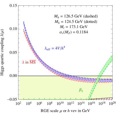
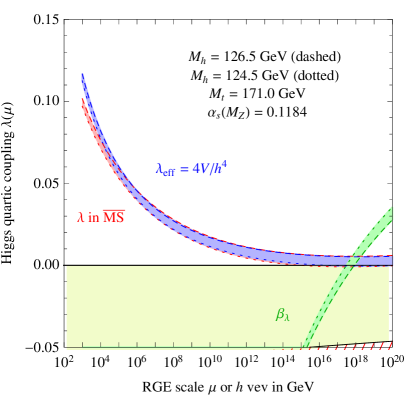
Figure 3: Evolution of the Higgs coupling λ(μ)𝜆𝜇\lambda(\mu) and its beta function, eq. (50), as a function of the renormalization scale, compared to the evolution of the effective coupling λeff(h)subscript𝜆eff\lambda_{\rm eff}(h), defined in eq. (51), as a function of the field value. Left: curves plotted for the best-fit value of Mtsubscript𝑀𝑡M_{t}. Right: curves plotted for the lower value of Mtsubscript𝑀𝑡M_{t} that corresponds to λ(MPl)=0𝜆subscript𝑀Pl0\lambda(M_{\rm Pl})=0.

The difference λeff(h)λ(h)subscript𝜆eff𝜆\lambda_{\rm eff}(h)-\lambda(h) is positive, as illustrated in fig. 3. As a result [9], at a given field value the potential is more stable than what guessed from the naive expectation based on the RG-improved tree-level potential in eq. (49), with μ=h𝜇\mu=h. We finally notice that the difference λeff(h)λ(h)subscript𝜆eff𝜆\lambda_{\rm eff}(h)-\lambda(h) gets suppressed at large field values, especially when λ𝜆\lambda reaches its minimum close to the Planck scale. This is expected according to the following two observations: 1) the difference between λeffsubscript𝜆eff\lambda_{\rm eff} and λ𝜆\lambda can be reabsorbed by a shift in the scales at which the two couplings are evaluated, up to finite two-loop corrections; 2) this shift has a small impact at large field values given the corresponding vanishing of βλsubscript𝛽𝜆\beta_{\lambda} (see fig. 3).

3.2 Inputs at the electroweak scale and threshold corrections

As far as the SM gauge couplings are concerned, we can directly use results in the literature for the couplings in the MS¯¯MS\overline{\rm MS} scheme. In particular, from a global fit of electroweak precision data, performed with the additional input Mh125GeVsubscript𝑀125GeVM_{h}\approx 125\,\mathrm{GeV}, the following MS¯¯MS\overline{\rm MS} values of the electromagnetic coupling and the weak angle renormalized at MZsubscript𝑀𝑍M_{Z} are obtained [32]:

αem1=127.937±0.015,sin2θW=0.23126±0.00005.formulae-sequencesuperscriptsubscript𝛼em1plus-or-minus127.9370.015superscript2subscript𝜃Wplus-or-minus0.231260.00005\alpha_{\rm em}^{-1}=127.937\pm 0.015~{},\qquad\sin^{2}\theta_{\rm W}=0.23126\pm 0.00005~{}. (55)

From these we derive

α21(MZ)=αem1sin2θW=29.587±0.008,superscriptsubscript𝛼21subscript𝑀𝑍superscriptsubscript𝛼em1superscript2subscript𝜃Wplus-or-minus29.5870.008\alpha_{2}^{-1}(M_{Z})=\alpha_{\rm em}^{-1}\sin^{2}\theta_{\rm W}=29.587\pm 0.008~{}, (56)
αY1(MZ)=αem1cos2θW=98.35±0.013.superscriptsubscript𝛼𝑌1subscript𝑀𝑍superscriptsubscript𝛼em1superscript2subscript𝜃Wplus-or-minus98.350.013\alpha_{Y}^{-1}(M_{Z})=\alpha_{\rm em}^{-1}\cos^{2}\theta_{\rm W}=98.35\pm 0.013\ . (57)

For the strong coupling we adopt

αs(MZ)=0.1184±0.0007[33]subscript𝛼𝑠subscript𝑀𝑍plus-or-minus0.11840.0007[33]\alpha_{s}(M_{Z})=0.1184\pm 0.0007~{}\hbox{\cite[cite]{[\@@bibref{}{alpha3}{}{}]}} (58)

such that, including 3 loop RG running up to Mtsubscript𝑀𝑡M_{t} and matching to the theory with 6 flavors, we get

gs(Mt)=1.1645+0.0031(αs(MZ)0.11840.0007)0.00046(MtGeV173.15).subscript𝑔𝑠subscript𝑀𝑡1.16450.0031subscript𝛼𝑠subscript𝑀𝑍0.11840.00070.00046subscript𝑀𝑡GeV173.15g_{s}(M_{t})=1.1645+0.0031\left(\frac{\alpha_{s}(M_{Z})-0.1184}{0.0007}\right)-0.00046\left(\frac{M_{t}}{\,\mathrm{GeV}}-173.15\right). (59)

We determine the MS¯¯MS\overline{\rm MS} top-quark Yukawa coupling (ytsubscript𝑦𝑡y_{t}) starting from the top-quark pole mass (Mtsubscript𝑀𝑡M_{t}) determined from experiments. Averaging measurements from Tevatron and LHC experiments,

Mt={173.2±0.9GeVTevatron [34]172.6±0.6±1.2GeVCMS μj [35]174.5±0.6±2.3GeVATLAS j [36],subscript𝑀𝑡casesplus-or-minus173.20.9GeVTevatron [34]plus-or-minus172.60.61.2GeVCMS μj [35]plus-or-minus174.50.62.3GeVATLAS j [36]M_{t}=\left\{\begin{array}[]{ll}173.2\pm 0.9~{}{\rm GeV}&\hbox{Tevatron~{}\hbox{\cite[cite]{[\@@bibref{}{topmass}{}{}]}}}\\ 172.6\pm 0.6\pm 1.2~{}{\rm GeV}&\hbox{CMS $\mu j$~{}\cite[cite]{[\@@bibref{}{MtCMS}{}{}]}}\\ 174.5\pm 0.6\pm 2.3~{}{\rm GeV}&\hbox{ATLAS $\ell j$~{}\cite[cite]{[\@@bibref{}{MtATLAS}{}{}]}},\end{array}\right. (60)

we get

Mt=(173.1±0.7)GeV.subscript𝑀𝑡plus-or-minus173.10.7GeVM_{t}=(173.1\pm 0.7)\,\mathrm{GeV}~{}. (61)

In order to translate this value into a determination of ytsubscript𝑦𝑡y_{t} we apply: 1) QCD threshold corrections up to O(αs3)𝑂superscriptsubscript𝛼𝑠3O(\alpha_{s}^{3}) [37, 38]; 2) complete one-loop electroweak corrections from ref. [39]; 3) two-loop 𝒪(ααs)𝒪𝛼subscript𝛼𝑠{\cal O}(\alpha\alpha_{s}) corrections from ref. [40], including the 𝒪(ααs)𝒪𝛼subscript𝛼𝑠{\cal O}(\alpha\alpha_{s}) terms due to the renormalization of the Fermi coupling (see sect. 2). As a result, we find, for the MS¯¯MS\overline{\rm MS} top Yukawa coupling renormalized at the top pole mass Mtsubscript𝑀𝑡M_{t}:

yt(Mt)subscript𝑦𝑡subscript𝑀𝑡\displaystyle y_{t}(M_{t}) =\displaystyle= 0.93587+0.00557(MtGeV173.15)0.00003(MhGeV125)0.935870.00557subscript𝑀𝑡GeV173.150.00003subscript𝑀GeV125\displaystyle 0.93587+0.00557\left(\frac{M_{t}}{\,\mathrm{GeV}}-173.15\right)-0.00003\left(\frac{M_{h}}{\,\mathrm{GeV}}-125\right) (62)
0.00041(αs(MZ)0.11840.0007)±0.00200th.plus-or-minus0.00041subscript𝛼𝑠subscript𝑀𝑍0.11840.0007subscript0.00200th\displaystyle-0.00041\left(\frac{\alpha_{s}(M_{Z})-0.1184}{0.0007}\right)\pm 0.00200_{\rm th}~{}.

The 𝒪(ααs)𝒪𝛼subscript𝛼𝑠{\cal O}(\alpha\alpha_{s}) term, that is the parametrically smallest correction, is equivalent to a tiny shift in Mtsubscript𝑀𝑡M_{t} below 0.10.10.1 GeV. This effect is well below the 𝒪(ΛQCD)𝒪subscriptΛQCD{\cal O}(\Lambda_{\rm QCD}) irreducible non-perturbative uncertainty on the top-quark mass determined at hadron colliders (see e.g. ref. [41, 42]), that is responsible for the theoretical error in eq. (62). More explicitly, we estimate an irreducible theoretical error of ±ΛQCD±0.3GeVplus-or-minussubscriptΛQCDplus-or-minus0.3GeV\pm\Lambda_{\rm QCD}\approx\pm 0.3\,\mathrm{GeV} in Mtsubscript𝑀𝑡M_{t} from non-perturbative effects, and an additional uncertainty of ±0.15GeVplus-or-minus0.15GeV\pm 0.15\,\mathrm{GeV} from missing 𝒪(αs4)𝒪subscriptsuperscript𝛼4𝑠{\cal O}(\alpha^{4}_{s}) threshold corrections.333 In principle, a direct determination of the MS¯¯MS\overline{\rm MS} top-quark mass at hadron colliders can be obtained from the experimental data on the σ(pp/pp¯tt¯)𝜎𝑝𝑝𝑝¯𝑝𝑡¯𝑡\sigma(pp/p\bar{p}\to t\bar{t}) cross section (see ref. [43] and references therein). At present this determination leads to a value for Mtsubscript𝑀𝑡M_{t} which is perfectly consistent with eq. (61) but has an error four times larger [44]. For completeness and for future reference, we report here the stability condition in eq. (2) as a function of the MS¯¯MS\overline{\rm MS} top-quark Yukawa coupling, rather than the top-quark pole mass: Mh[GeV]>129.4+2.0(yt(Mt)0.93560.0054)0.35(αs(MZ)0.11840.0007)±1.0th.subscript𝑀delimited-[]GeVplus-or-minus129.42.0subscript𝑦𝑡subscript𝑀𝑡0.93560.00540.35subscript𝛼𝑠subscript𝑀𝑍0.11840.0007subscript1.0thM_{h}~{}[{\rm GeV}]>129.4+2.0\left(\frac{y_{t}(M_{t})-0.9356}{0.0054}\right)-0.35\left(\frac{\alpha_{s}(M_{Z})-0.1184}{0.0007}\right)\pm 1.0_{\rm th}\ .

Next, applying the threshold corrections discussed in section 2, we determine the following value for the Higgs self coupling in the MS¯¯MS\overline{\rm MS} scheme renormalized at the pole top mass:

λ(Mt)=0.12577+0.00205(MhGeV125)0.00004(MtGeV173.15)±0.00140th.𝜆subscript𝑀𝑡plus-or-minus0.125770.00205subscript𝑀GeV1250.00004subscript𝑀𝑡GeV173.15subscript0.00140th\lambda(M_{t})=0.12577+0.00205\left(\frac{M_{h}}{\,\mathrm{GeV}}-125\right)-0.00004\left(\frac{M_{t}}{\,\mathrm{GeV}}-173.15\right)\pm 0.00140_{\rm th}~{}. (63)

The residual theoretical uncertainty, that is equivalent to an error of ±0.7plus-or-minus0.7\pm 0.7 GeV in Mhsubscript𝑀M_{h}, has been estimated varying the low-energy matching scale for λ𝜆\lambda between MZsubscript𝑀𝑍M_{Z} and 2Mt2subscript𝑀𝑡2M_{t}.

For completeness, we also include in the one- and two-loop RG equation the contributions of the small bottom and tau Yukawa couplings, as computed from the MS¯¯MS\overline{\rm MS} b𝑏b-quark mass, mb(mb)=4.2GeVsubscript𝑚𝑏subscript𝑚𝑏4.2GeVm_{b}(m_{b})=4.2\,\mathrm{GeV}, and from Mτ=1.777GeVsubscript𝑀𝜏1.777GeVM_{\tau}=1.777\,\mathrm{GeV}.

3.3 Phase diagram of the SM

Refer to caption      Refer to caption
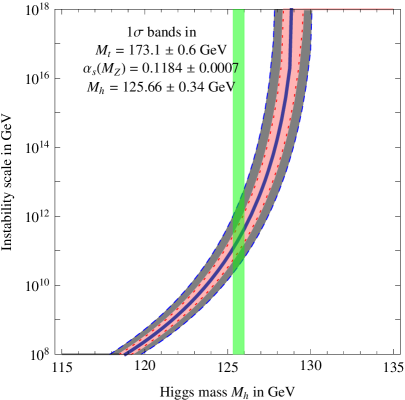
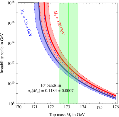
Figure 4: The instability scale ΛIsubscriptΛ𝐼\Lambda_{I} at which the SM potential becomes negative as a function of the Higgs mass (left) and of the top mass (right). The theoretical error is not shown and corresponds to a ±1GeVplus-or-minus1GeV\pm 1\,\mathrm{GeV} uncertainty in Mhsubscript𝑀M_{h}.

The final result for the condition of absolute stability is presented in eq. (2). The central value of the stability bound at NNLO on Mhsubscript𝑀M_{h} is shifted with respect to NLO computations (where the matching scale is fixed at μ=Mt𝜇subscript𝑀𝑡\mu=M_{t}) by about +0.5GeV0.5GeV+0.5\,\mathrm{GeV}, whose main contributions can be decomposed as follows:
+0.6GeV0.6GeV~{}\qquad+0.6\,\mathrm{GeV} due to the QCD threshold corrections to λ𝜆\lambda (in agreement with [20]);
+0.2GeV0.2GeV~{}\qquad+0.2\,\mathrm{GeV} due to the Yukawa threshold corrections to λ𝜆\lambda;
0.2GeV0.2GeV~{}\qquad-0.2\,\mathrm{GeV} from RG equation at 3 loops (from [18, 19]);
0.1GeV0.1GeV~{}\qquad-0.1\,\mathrm{GeV} from the effective potential at 2 loops.
As a result of these corrections, the instability scale is lowered by a factor 2similar-toabsent2\sim 2, for Mh125similar-tosubscript𝑀125M_{h}\sim 125 GeV, after including NNLO effects. The value of the instability scale is shown in fig. 4.
Refer to caption      Refer to caption
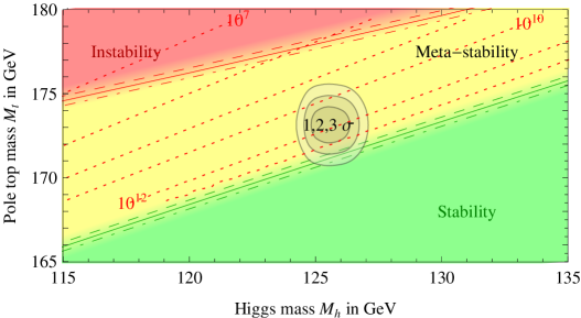
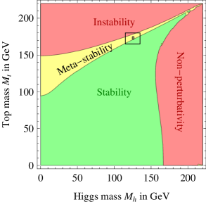
Figure 5: Regions of absolute stability, meta-stability and instability of the SM vacuum in the Mtsubscript𝑀𝑡M_{t}Mhsubscript𝑀M_{h} plane (upper left) and in the λ𝜆\lambdaytsubscript𝑦𝑡y_{t} plane, in terms of parameter renormalized at the Planck scale (upper right). Bottom: Zoom in the region of the preferred experimental range of Mhsubscript𝑀M_{h} and Mtsubscript𝑀𝑡M_{t} (the gray areas denote the allowed region at 1, 2, and 3σ𝜎\sigma). The three boundary lines correspond to αs(MZ)=0.1184±0.0007subscript𝛼𝑠subscript𝑀𝑍plus-or-minus0.11840.0007\alpha_{s}(M_{Z})=0.1184\pm 0.0007, and the grading of the colors indicates the size of the theoretical error. The dotted contour-lines show the instability scale ΛΛ\Lambda in GeVGeV\,\mathrm{GeV} assuming αs(MZ)=0.1184subscript𝛼𝑠subscript𝑀𝑍0.1184\alpha_{s}(M_{Z})=0.1184.

The phase diagram of the SM Higgs potential is shown in fig. 5, taking into account the values for Mhsubscript𝑀M_{h} measured by ATLAS and CMS [1, 2]. The left plot illustrates the remarkable coincidence for which the SM appears to live right at the border between the stability and instability regions. As can be inferred from the bottom plot, which zooms into the relevant region, there is significant preference for meta-stability of the SM potential. By taking into account all uncertainties, we find that the stability region is disfavored by present data by 2σ2𝜎2\sigma. For Mh<126subscript𝑀126M_{h}<126 GeV, stability up to the Planck mass is excluded at 98% C.L. (one sided).

Type of error Estimate of the error Impact on Mhsubscript𝑀M_{h}
Mtsubscript𝑀𝑡M_{t} experimental uncertainty in Mtsubscript𝑀𝑡M_{t} ±1.4plus-or-minus1.4\pm 1.4 GeV
αssubscript𝛼s\alpha_{\rm s} experimental uncertainty in αssubscript𝛼s\alpha_{\rm s} ±0.5plus-or-minus0.5\pm 0.5 GeV
Experiment Total combined in quadrature ±1.5plus-or-minus1.5\pm 1.5 GeV
λ𝜆\lambda scale variation in λ𝜆\lambda ±0.7plus-or-minus0.7\pm 0.7 GeV
ytsubscript𝑦𝑡y_{t} 𝒪(ΛQCD)𝒪subscriptΛQCD{\cal O}(\Lambda_{\rm QCD}) correction to Mtsubscript𝑀𝑡M_{t} ±0.6plus-or-minus0.6\pm 0.6 GeV
ytsubscript𝑦𝑡y_{t} QCD threshold at 4 loops ±0.3plus-or-minus0.3\pm 0.3 GeV
RGE EW at 3 loops + QCD at 4 loops ±0.2plus-or-minus0.2\pm 0.2 GeV
Theory Total combined in quadrature ±1.0plus-or-minus1.0\pm 1.0 GeV
Table 1: Dominant sources of experimental and theoretical errors in the computation of the SM stability bound on the Higgs mass, eq. (2).

The dominant uncertainties in the evaluation of the minimum Mhsubscript𝑀M_{h} value ensuring absolute vacuum stability within the SM are summarized in Table 1. The dominant uncertainty is experimental and comes mostly from the measurement of Mtsubscript𝑀𝑡M_{t}. Although experiments at the LHC are expected to improve the determination of Mtsubscript𝑀𝑡M_{t}, the error on the top mass will remain as the largest source of uncertainty. If no new physics other than the Higgs boson is discovered at the LHC, the peculiarity of having found that the SM parameters lie at the critical border between stability and metastability regions provides a valid motivation for improved top quark mass measurements, possibly at a linear collider.

The dominant theoretical uncertainty, while reduced by about a factor of 3 with the present work, is still related to threshold corrections to the Higgs coupling λ𝜆\lambda at the weak scale. Another sizable theoretical uncertainty comes from the fact that the pole top mass determined at hadron colliders suffers from 𝒪(ΛQCD)𝒪subscriptΛQCD{\cal O}(\Lambda_{\rm QCD}) non-perturbative uncertainties [41]. A possibility to overcome this problem and, at the same time, to improve the experimental error on Mtsubscript𝑀𝑡M_{t}, would be a direct determination of the MS¯¯MS\overline{\rm MS} top-quark running mass from experiments, for instance from the tt¯𝑡¯𝑡t\bar{t} cross-section at a future e+esuperscript𝑒superscript𝑒e^{+}e^{-} collider operating above the tt¯𝑡¯𝑡t\bar{t} threshold. In this respect, such a collider could become crucial for establishing the structure of the vacuum and the ultimate fate of our universe.

As far as the RG equations are concerned, the error of ±0.2plus-or-minus0.2\pm 0.2 GeV is a conservative estimate, based on the parametric size of the missing terms. The smallness of this error, compared to the uncertainty due to threshold corrections, can be understood by the smallness of all the couplings at high scales: four-loop terms in the RG equations do not compete with finite tree-loop corrections close to the electroweak scale, where the strong and the top-quark Yukawa coupling are large.

The LHC will be able to measure the Higgs mass with an accuracy of about 100–200 MeV, which is far better than the theoretical error with which we are able to determine the condition of absolute stability.
Refer to caption      Refer to caption
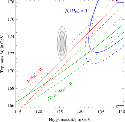
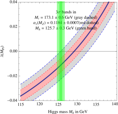
Figure 6: Left: The Higgs quartic coupling λ𝜆\lambda at the Planck scale as a function of Mhsubscript𝑀M_{h}, with ±3σplus-or-minus3𝜎\pm 3\sigma variations in Mtsubscript𝑀𝑡M_{t} and αssubscript𝛼s\alpha_{\rm s}. Right: Curves in the Mtsubscript𝑀𝑡M_{t}Mhsubscript𝑀M_{h} plane corresponding to the conditions λ(MPl)=0𝜆subscript𝑀Pl0\lambda(M_{\rm Pl})=0 (red), βλ(MPl)=0subscript𝛽𝜆subscript𝑀Pl0\beta_{\lambda}(M_{\rm Pl})=0 (blue), and to the Veltman’s condition of vanishing supertrace (green, see text). In all cases the dashed and dotted lines denote the ±3σplus-or-minus3𝜎\pm 3\sigma variation in αssubscript𝛼s\alpha_{\rm s}. The gray areas denote the experimentally allowed region at 1, 2, and 3σ𝜎\sigma.

4 Implications

4.1 Boundary conditions at the Planck scale

It is certainly a remarkable coincidence that both λ𝜆\lambda and its beta function βλsubscript𝛽𝜆\beta_{\lambda} nearly vanish around the Planck scale. This motivates us to explore in more detail the boundary conditions at MPlsubscript𝑀PlM_{\rm Pl} required to reproduce the measured values of the SM parameters. In fig. 6 (left) we show the prediction for the Higgs quartic coupling λ𝜆\lambda at MPlsubscript𝑀PlM_{\rm Pl}, with 3σ𝜎\sigma bands describing the errors in Mtsubscript𝑀𝑡M_{t} and αssubscript𝛼𝑠\alpha_{s}. For Mhsubscript𝑀M_{h} in the range preferred by LHC, λ(MPl)=0𝜆subscript𝑀Pl0\lambda(M_{\rm Pl})=0 can be obtained only if Mtsubscript𝑀𝑡M_{t} is 2absent2\approx 2 GeV below its present central value (i.e. Mt171subscript𝑀𝑡171M_{t}\leq 171 GeV). However, it should be noted that λ=0𝜆0\lambda=0 is neither a fixed point nor a point of enhanced symmetry and thus satisfying exactly this condition is not especially meaningful. The best-fit value for λ𝜆\lambda at the Planck scale is small and negative,

λ(MPl)=0.0129+0.0028(MhGeV125.5)±0.0047Mt±0.0018αs±0.0028th,𝜆subscript𝑀Plplus-or-minus0.01290.0028subscript𝑀GeV125.5subscript0.0047subscript𝑀𝑡subscript0.0018subscript𝛼𝑠subscript0.0028th\lambda(M_{\rm Pl})=-0.0129+0.0028\left(\frac{M_{h}}{\,\mathrm{GeV}}-125.5\right)\pm 0.0047_{M_{t}}\pm 0.0018_{\alpha_{s}}\pm 0.0028_{\rm th}\ , (64)

where the uncertainties refer to the present 1σ1𝜎1\sigma errors in Mtsubscript𝑀𝑡M_{t} and αssubscript𝛼s\alpha_{\rm s}, and to the theoretical error.

Equation (64) could be the result of matching the SM at MPlsubscript𝑀PlM_{\rm Pl} with a theory in which λ𝜆\lambda vanishes at tree level and receives one-loop threshold corrections. However, the contribution to high-energy thresholds from the SM couplings at MPlsubscript𝑀PlM_{\rm Pl} is typically a few times 103superscript10310^{-3}. The required effect of size 102superscript10210^{-2} can be obtained from loops of SM couplings only if these involve particles with large multiplicities, or else from loop with new (large) coupling constants. As evident from fig. 1, the boundary condition of λ𝜆\lambda at high energy is fairly independent of the precise value at which we impose it.

The right plot in fig. 6 shows the dependence on Mhsubscript𝑀M_{h} and Mtsubscript𝑀𝑡M_{t} of the boundary conditions λ(MPl)=0𝜆subscript𝑀Pl0\lambda(M_{\rm Pl})=0 (red line) and βλ(MPl)=0subscript𝛽𝜆subscript𝑀Pl0\beta_{\lambda}(M_{\rm Pl})=0 (blue line). While λ=0𝜆0\lambda=0 weakly depends on the scale at which is evaluated, a more pronounced dependence affects the condition βλ=0subscript𝛽𝜆0\beta_{\lambda}=0 (see fig. 3). This is because βλsubscript𝛽𝜆\beta_{\lambda} depends not only on λ𝜆\lambda, but also on other couplings (top Yukawa and gauge) that run in the high-energy region. As a result, although βλ(MPl)=0subscript𝛽𝜆subscript𝑀Pl0\beta_{\lambda}(M_{\rm Pl})=0 cannot be exactly satisfied, the beta function vanishes at scales very near the Planck mass. For instance, for Mt=171.0subscript𝑀𝑡171.0M_{t}=171.0 GeV and Mh=125subscript𝑀125M_{h}=125 GeV, both λ𝜆\lambda and βλsubscript𝛽𝜆\beta_{\lambda} simultaneously vanish when they are evaluated at a scale equal to 3×10¹⁷GeV3superscript1017GeV3\times 10^{17}\,\mathrm{GeV}. In ref. [22] it was argued that λ(MPl)0𝜆subscript𝑀Pl0\lambda(M_{\rm Pl})\approx 0 and βλ(MPl)0subscript𝛽𝜆subscript𝑀Pl0\beta_{\lambda}(M_{\rm Pl})\approx 0 could be justified in the case of an asymptotically safe gravitational theory.

Just for illustration, in the right plot in fig. 6 we also show the Higgs mass implied by Veltman’s condition [45] that the supertrace of the squared masses of all SM particles vanishes at a given scale, here chosen to be MPlsubscript𝑀PlM_{\rm Pl}: STr2(MPl)=0STrsuperscript2subscript𝑀Pl0{\rm STr}{\cal M}^{2}(M_{\rm Pl})=0. We remark, however, that this condition does not carry special information about the power divergences of the theory, which are dominated by UV effects, while the supertrace includes only the contribution from the IR degrees of freedom in the SM. At any rate, the possibility of a very special fine-tuning involving only the SM loop contributions and leading to STr2(MPl)=0STrsuperscript2subscript𝑀Pl0{\rm STr}{\cal M}^{2}(M_{\rm Pl})=0, implies a Higgs mass Mh(135±2.5)GeVsubscript𝑀plus-or-minus1352.5GeVM_{h}\approx(135\pm 2.5)\,\mathrm{GeV}, which is excluded at more than 3σ𝜎\sigma. Lowering the scale at which the supertrace condition is evaluated makes the disagreement even stronger.

4.2 Higgs inflation from non-minimal coupling to gravity

The extrapolation of the SM up to very high energy has led to some speculations about the possibility of interpreting the Higgs boson as the inflaton. One scenario for Higgs inflation [46] exploits a large non-minimal coupling between the Higgs bilinear and the Ricci scalar R𝑅R, with an interaction Lagrangian ξ|H|2R𝜉superscript𝐻2𝑅\xi|H|^{2}R. The effect of this interaction is to flatten the Higgs potential (or any other potential) above the scale MPl/ξsubscript𝑀Pl𝜉M_{\rm Pl}/\sqrt{\xi}, providing a platform for slow-roll inflation. A correct normalization of the spectrum of primordial fluctuations fixes the value of the coupling constant ξ𝜉\xi. Using the tree-level potential, one finds ξ5×10⁴λ𝜉5superscript104𝜆\xi\approx 5\times 10^{4}\sqrt{\lambda}.

This inflationary scenario, attractive for its minimality, suffers from a serious drawback. Perturbative unitarity is violated at the scale MPl/ξsubscript𝑀Pl𝜉M_{\rm Pl}/\xi, signaling the presence of new physical phenomena associated with strong dynamics. It is naturally expected that these phenomena will affect the scalar potential above MPl/ξsubscript𝑀Pl𝜉M_{\rm Pl}/\xi in an uncontrollable way [47]. One solution is to add new degrees of freedom that restore perturbative unitarity [48], although the minimality of the model is then lost. The procedure advocated by the proponents of this scenario is to assume that the strong dynamics will preserve intact the shape of the SM potential, even above MPl/ξsubscript𝑀Pl𝜉M_{\rm Pl}/\xi. Although we find this assumption questionable, it is still interesting to address the issue of whether the Higgs data are compatible with this scenario.

A two-loop analysis of Higgs ξ𝜉\xi-inflation was developed in ref. [14, 49]. The ordinary SM evolution is perfectly adequate below the scale MPl/ξsubscript𝑀Pl𝜉M_{\rm Pl}/\xi, while the new interaction can affect the scalar potential at very high energy. The renormalization procedure above the inflationary scale is not unambiguous as, for instance, the renormalization scale differs in the Jordan and Einstein frames. Luckily, the slow running of λ𝜆\lambda at high energy makes these issues irrelevant, from a practical point of view. A simple SM calculation of the potential is perfectly adequate to describe the situation of Higgs ξ𝜉\xi-inflation (see also the discussion in ref. [20]).

In practice, the result is that Higgs ξ𝜉\xi-inflation requires stability of the potential up to the inflationary scale MPl/ξsubscript𝑀Pl𝜉M_{\rm Pl}/\sqrt{\xi}. As we are interested in the minimum value of the Higgs mass that satisfies this condition, the coupling λ𝜆\lambda at the relevant scale is very small and thus the coupling ξ𝜉\xi is not particularly large, ξ<𝒪(103)𝜉𝒪superscript103\xi<{\cal O}(10^{3}). Therefore, the resulting restriction is stability, as given by eq. (2). If the LHC indication for Mh=125subscript𝑀125M_{h}=125–126 GeV is confirmed, the simplest version of Higgs inflation is disfavored, unless the top mass is about 2σ𝜎\sigma below its present central value. However, given the proximity of λ(MPl)𝜆subscript𝑀Pl\lambda(M_{\rm Pl}) to the critical value for stability, unknown one-loop threshold corrections near the Planck mass could be sufficient to rescue the proposal. It is also interesting that the introduction of a single scalar field at the scale MPl/ξsubscript𝑀Pl𝜉M_{\rm Pl}/\xi could simultaneously restore perturbative unitarity and cure the potential instability [50].

4.3 Higgs inflation from false vacuum

Alternative proposals for Higgs inflation employ the peculiarity of the SM scalar potential to develop a second minimum at large Higgs field values for a very special choice of parameters [21, 11]. The possibility of using this new minimum for inflation was first contemplated in ref. [12], finding that it implies a viable prediction for the Higgs mass, but also a wrong prediction for the amplitude of density fluctuations. The latter result can be cured in non-minimal inflationary setups [24, 25] without affecting the prediction for the Higgs mass, which we now precisely compute.

The first derivative of the Higgs potential V=λeff(h)h4/4𝑉subscript𝜆effsuperscript44V=\lambda_{\rm eff}(h)h^{4}/4 is

dVdh=(λeff+βeff4)h3.𝑑𝑉𝑑subscript𝜆effsubscript𝛽eff4superscript3\frac{dV}{dh}=\left(\lambda_{\rm eff}+\frac{\beta_{\rm eff}}{4}\right)h^{3}~{}. (65)

Here λeff(h)subscript𝜆eff\lambda_{\rm eff}(h) is the effective coupling defined in eq. (3.1) and βeff=dλeff/dlnhsubscript𝛽eff𝑑subscript𝜆eff𝑑\beta_{\rm eff}=d\lambda_{\rm eff}/d\ln h. If λeffsubscript𝜆eff\lambda_{\rm eff} becomes sufficiently small, the potential can develop a minimum at h=hminsubscriptminh=h_{\rm min}, such that

λeff+βeff4|h=hmin=0.subscript𝜆effevaluated-atsubscript𝛽eff4subscriptmin0\left.\lambda_{\rm eff}+\frac{\beta_{\rm eff}}{4}\right|_{h=h_{\rm min}}=0~{}. (66)

This situation can occur in the proximity of a field value hsubscripth_{*} where βeffsubscript𝛽eff\beta_{\rm eff} vanishes. In the neighborhood of hsubscripth_{*}, we can approximate λeff(h)subscript𝜆eff\lambda_{\rm eff}(h) as

λeff(h)λ+bln2hh,subscript𝜆effsubscript𝜆𝑏superscript2subscript\lambda_{\rm eff}(h)\approx\lambda_{*}+b\ln^{2}\frac{h}{h_{*}}~{}, (67)

where λsubscript𝜆\lambda_{*} is the minimum value of λeffsubscript𝜆eff\lambda_{\rm eff}, such that βeff(λ)=0subscript𝛽effsubscript𝜆0\beta_{\rm eff}(\lambda_{*})=0. The zero of the β𝛽\beta function insures that the leading log is absent in eq. (67) and thus b𝑏b is a typical two-loop coefficient. For the relevant values of the SM parameters, we find b=0.4/(4π)4𝑏0.4superscript4𝜋4b=0.4/(4\pi)^{4}. We are interested in a situation in which the field configuration corresponds to a local minimum (while the EW vacuum remains the global minimum) and thus we want both λsubscript𝜆\lambda_{*} and b𝑏b to be positive. Using the expansion in eq. (67), we can compute hminsubscriptminh_{\rm min} and the minimum of the potential VminV(hmin)subscript𝑉min𝑉subscriptminV_{\rm min}\equiv V(h_{\rm min}),

hminhexp[14(116λb1)],subscriptminsubscript14116subscript𝜆𝑏1h_{\rm min}\approx h_{*}\exp\left[\frac{1}{4}\left(\sqrt{1-\frac{16\lambda_{*}}{b}}-1\right)\right]~{}, (68)
Vminb8hmin4lnhhmin.subscript𝑉min𝑏8superscriptsubscriptmin4subscriptsubscriptminV_{\rm min}\approx\frac{b}{8}~{}h_{\rm min}^{4}\ln\frac{h_{*}}{h_{\rm min}}~{}. (69)

The minimum hminsubscriptminh_{\rm min} exists only for extremely small values of the Higgs quartic coupling, λ<b/16subscript𝜆𝑏16\lambda_{*}<b/16. As we vary λsubscript𝜆\lambda_{*} within its allowed range (0<λ<b/160subscript𝜆𝑏160<\lambda_{*}<b/16) we find that hminsubscriptminh_{\rm min} is always near hsubscripth_{*} (e1/4<hmin/h<1superscript𝑒14subscriptminsubscript1e^{-1/4}<h_{\rm min}/h_{*}<1), while Vminsubscript𝑉minV_{\rm min} can change widely (0<Vmin<bhmin4/320subscript𝑉min𝑏superscriptsubscriptmin4320<V_{\rm min}<bh_{\rm min}^{4}/32).

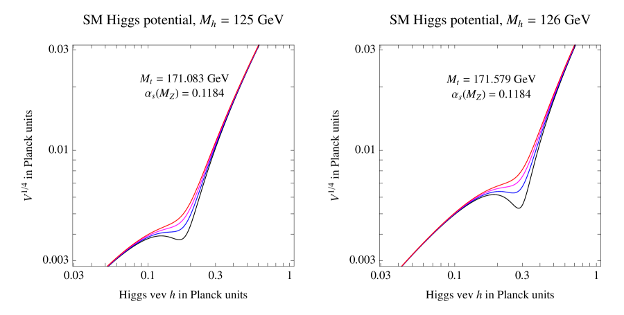
If the Higgs field is trapped in the false vacuum during the early universe, it can cause inflation. The normalization of the spectrum of primordial perturbations, which is determined by Vminsubscript𝑉minV_{\rm min}, can be appropriately selected by tuning the ratio λ/bsubscript𝜆𝑏\lambda_{*}/b. The main difficulty of this scenario is to achieve a graceful exit from the inflationary phase. Two mechanisms have been proposed. The first one [24] employs a new scalar field, non-minimally coupled to gravity, that slows down the expansion rate, thus allowing for quantum tunneling of the Higgs out of the false vacuum. The second mechanism [25] uses a scalar field weakly coupled to the Higgs which, during the cosmological evolution, removes the barrier in the Higgs potential in a process analogous to hybrid inflation. So, in practice, the minimality of the SM is lost and one may wonder if there is any conceptual gain with respect to adding a new scalar playing the role of the inflaton. Nevertheless, it is interesting to investigate whether the Higgs and top masses are compatible with the intriguing possibility of a false vacuum at large field value.
Refer to caption
Figure 7: Two-loop SM Higgs potential for Mh=125,126GeVsubscript𝑀125126GeVM_{h}=125,126\,\mathrm{GeV} around the critical top mass that gives a second minimum around the Planck scale. The various curves correspond to variations in Mtsubscript𝑀𝑡M_{t} by 0.1MeV0.1MeV0.1\,\mathrm{MeV}.

In practice the above equations amount to saying that the conditions for the existence of a second (unstable) vacuum are that λeffsubscript𝜆eff\lambda_{\rm eff} (essentially) vanishes at the same scale at which βeffsubscript𝛽eff\beta_{\rm eff} vanishes. This corresponds to the intersection between the red band (condition λλeff=0)\lambda\approx\lambda_{\rm eff}=0) and the blue band (condition βλ=0)\beta_{\lambda}=0) in fig. 6(right). It is remarkable that the SM can achieve these conditions, although they require a top mass about 2σ𝜎\sigma below the central value. The resulting relation between Mhsubscript𝑀M_{h} and Mtsubscript𝑀𝑡M_{t} corresponds to the equality in eq. (2), and is precisely studied in fig. 7 where we compute for Mh={125,126}GeVsubscript𝑀125126GeVM_{h}=\{125,126\}\,\mathrm{GeV} the predicted top mass and show the shape of the potential around the false vacuum. The value of Vminsubscript𝑉minV_{\rm min} can be changed by tuning λsubscript𝜆\lambda_{*} or, in other words, by accurate variations of Mhsubscript𝑀M_{h} and Mtsubscript𝑀𝑡M_{t}. The existence of the false vacuum depends critically on the exact values of the SM parameters and requires dialing Mhsubscript𝑀M_{h} and Mtsubscript𝑀𝑡M_{t} by one part in 106superscript10610^{6}. However, the exact value of the needed top mass has a theoretical uncertainty, reduced down to ±0.5GeVplus-or-minus0.5GeV\pm 0.5\,\mathrm{GeV} thanks to our higher-order computation. Note from fig. 7 that the field value where the false vacuum is positioned is larger than what was reported in [12, 24]. The corrections in eq. (3.1) [9, 11] are mostly responsible for the larger field values found in our analysis.
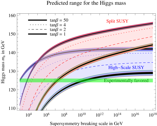
Refer to caption
Figure 8: NNLO prediction for the Higgs mass Mhsubscript𝑀M_{h} in High-Scale Supersymmetry (blue, lower) and Split Supersymmetry (red, upper) for tanβ={1,2,4,50}𝛽12450\tan\beta=\{1,2,4,50\}. The thickness of the lower boundary at tanβ=1𝛽1\tan\beta=1 and of the upper boundary at tanβ=50𝛽50\tan\beta=50 shows the uncertainty due to the present 1σ1𝜎1\sigma error on αssubscript𝛼𝑠\alpha_{s} (black band) and on the top mass (larger colored band).

4.4 Supersymmetry

Our higher order computation of the relation between the Higgs mass and the Higgs quartic coupling λ𝜆\lambda has implications for any model that can predict λ𝜆\lambda. If supersymmetry is present at some scale m~~𝑚\tilde{m}, then in the minimal model one finds the tree-level relation

λ(m~)=18[g2(m~)+g2(m~)]cos22β.𝜆~𝑚18delimited-[]superscript𝑔2~𝑚superscript𝑔2~𝑚superscript22𝛽\lambda({\tilde{m}})=\frac{1}{8}\left[g^{2}({\tilde{m}})+g^{\prime 2}({\tilde{m}})\right]\cos^{2}2\beta~{}. (70)

A dedicated analysis of the resulting prediction for the Higgs mass as function of m~~𝑚\tilde{m} and of tanβ𝛽\tan\beta was performed in [51] (see also [52]). We here update the results, including the new correction which increases the predicted Higgs mass by an amount that changes with Mhsubscript𝑀M_{h}. Once more, the main impact of our calculation is the reduction of the theoretical uncertainty from ±3GeVplus-or-minus3GeV\pm 3\,\mathrm{GeV} down to ±1GeVplus-or-minus1GeV\pm 1\,\mathrm{GeV}. As a consequence, supersymmetry broken at the Planck scale, which requires λ0𝜆0\lambda\geq 0 and thus the stability condition eq. (2), is disfavored at 2σ2𝜎2\sigma, unless thresholds at MPlsubscript𝑀PlM_{\rm Pl} (or non-minimal couplings) account for the small negative value of λ(MPl)𝜆subscript𝑀Pl\lambda(M_{\rm Pl}), see eq. (64). Thresholds at one loop have been computed in [51] including finite parts and the constant factor due to the fact that the MS¯¯MS\overline{\rm MS} renormalization scheme breaks supersymmetry. A simplified, but illustrative, formula for the supersymmetric threshold corrections is obtained by taking a common mass M2subscript𝑀2M_{2} for weak gauginos and higgsinos, and a common mass mt~subscript𝑚~𝑡m_{\tilde{t}} for the stops,

δλ(MPl)1(4π)2[0.25+0.12lnmt~M2+0.05lnmAM2],𝛿𝜆subscript𝑀Pl1superscript4𝜋2delimited-[]0.250.12subscript𝑚~𝑡subscript𝑀20.05subscript𝑚𝐴subscript𝑀2\delta\lambda(M_{\rm Pl})\approx\frac{1}{(4\pi)^{2}}\left[-0.25+0.12\ln\frac{m_{\tilde{t}}}{M_{2}}+0.05\ln\frac{m_{A}}{M_{2}}\right]~{}, (71)

where mAsubscript𝑚𝐴m_{A} is the mass of the Higgs pseudoscalar. The absence of a scale dependence in eq. (71) is a consequence of the approximate cancellation of βλsubscript𝛽𝜆\beta_{\lambda} around MPlsubscript𝑀PlM_{\rm Pl}. Negative values of the boundary condition for λ𝜆\lambda thus require stops lighter than higgsinos, winos, and bino. By using the full formula and allowing for each sparticle mass to vary by one order of magnitude above or below the average mass m~~𝑚{\tilde{m}} we find

0.006<λ(MPl)<0.002.0.006𝜆subscript𝑀Pl0.002-0.006<\lambda(M_{\rm Pl})<0.002~{}. (72)

This is insufficient to reach the central value of eq. (64) and thus indicates that supersymmetry has to be broken at a scale below MPlsubscript𝑀PlM_{\rm Pl}, if the Higgs mass has to match a supersymmetric boundary condition.

Our predictions for the Higgs mass as a function of the supersymmetry breaking scale m~~𝑚\tilde{m} are illustrated in fig. 8, in the case of High-Scale Supersymmetry (all supersymmetric particles with masses equal to m~~𝑚\tilde{m}) and Split Supersymmetry [53] (supersymmetric scalars with masses equal to m~~𝑚\tilde{m} and supersymmetric fermions at the weak scale). We refer the reader to ref. [51] for details about the underlying assumptions of the calculation.

Figure 8 shows not only how Mh125GeVsubscript𝑀125GeVM_{h}\approx 125\,\mathrm{GeV} disfavors supersymmetry broken at a very high scale, but also the well know fact that the usual scenario of weak-scale supersymmetry can account for the Higgs mass only for extreme values of the parameters (such as large tanβ𝛽\tan\beta, heavy stops, maximal stop mixing). In the case of Split Supersymmetry, large values of m~~𝑚\tilde{m} are clearly excluded by LHC Higgs searches. On the other hand, (mildly “unnatural”) scenarios in which the masses of supersymmetric scalars are one-loop larger than the weak scale [54] are in good agreement with data.

5 Conclusions

One of the most important questions addressed by the LHC is naturalness. Not only will the answer affect our understanding of the mechanism for EW breaking, but it will also determine our strategy for future directions in theoretical physics. On one side we have the avenue of larger symmetries unifying physical laws in a single fundamental principle; on the other side we have new kinds of paradigms, where parameters are not understood by naturalness arguments in the context of well-defined effective theories. At present, the multiverse is one of the most intriguing options to pursue the latter path.

If the LHC finds Higgs couplings deviating from the SM prediction and new degrees of freedom at the TeV scale, then the most important question will be to see if a consistent and natural (in the technical sense) explanation of EW breaking emerges from experimental data. But if the LHC discovers that the Higgs boson is not accompanied by any new physics, then it will be much harder for theorists to unveil the underlying organizing principles of nature. The multiverse, although being a stimulating physical concept, is discouragingly difficult to test from an empirical point of view. The measurement of the Higgs mass may provide a precious handle to gather some indirect information.

Once we extrapolate the SM to very short distances, we find that the values of the Higgs mass, hinted by the first LHC results (125–126 GeV), lie right at the edge between EW stability and instability regions, see fig. 5. Moreover, the slow running of the quartic Higgs coupling λ𝜆\lambda in the high-energy regime implies that the instability scale most critically depends on the Higgs mass Mhsubscript𝑀M_{h}. A small change in Mhsubscript𝑀M_{h} (and Mtsubscript𝑀𝑡M_{t}) can drastically modify our conclusions regarding vacuum stability. This special situation motivated us to perform a NNLO calculation of the Higgs potential in the SM, which is the subject of this paper.

Our calculation includes three-loop running for gauge, top Yukawa, and Higgs quartic coupling and two-loop matching conditions keeping the leading effects in αssubscript𝛼𝑠\alpha_{s}, ytsubscript𝑦𝑡y_{t} and λ𝜆\lambda. In particular, we have computed for the first time the two-loop threshold correction to λ𝜆\lambda, which was the most sizable missing ingredient of the NNLO result. The completion of the NNLO calculation allows us to reduce the theoretical error in the stability limit on the Higgs mass from 3 GeV to 1 GeV. Our final result is shown in eq. (2). After our calculation, the largest source of uncertainty comes from the parametric dependence on the top quark mass, which leads to a 1σ𝜎\sigma error of 1.4 GeV in the critical Higgs mass. Of course our calculation reliably accounts for IR effects, but ignores possible new (unknown) UV threshold effects occurring near the Planck scale. Since our goal is to learn information about physics at very short distances, the high-energy corrections constitute an opportunity, rather than a deficiency in the calculation.

The first lesson that we learn from the SM extrapolation is that the Higgs mass hinted by LHC results corresponds to λ0𝜆0\lambda\approx 0 and βλ0subscript𝛽𝜆0\beta_{\lambda}\approx 0 at high energies. This, by itself, is an intriguing result because λ=0𝜆0\lambda=0 is the critical value for stability and it may hide some information about Planckian physics. With our precise calculation, we can investigate further the situation. We find that, for Mh=125subscript𝑀125M_{h}=125 GeV, λ(MPl)=0.014±0.006𝜆subscript𝑀Plplus-or-minus0.0140.006\lambda(M_{\rm Pl})=-0.014\pm 0.006, see eq. (64). The exact vanishing of λ(MPl)𝜆subscript𝑀Pl\lambda(M_{\rm Pl}) is excluded at 2σ𝜎\sigma. Moreover, the smallness of βλsubscript𝛽𝜆\beta_{\lambda} at high energy implies that λ𝜆\lambda remains negative in a relatively large energy range. Indeed, we find that, for Mh=125subscript𝑀125M_{h}=125 GeV, the instability scale develops at 1011±1superscript10plus-or-minus11110^{11\pm 1} GeV. Quantum tunneling is sufficiently slow to ensure at least metastability of the EW vacuum, see fig. 5. The small value of λ(MPl)𝜆subscript𝑀Pl\lambda(M_{\rm Pl}) may indicate a radiative origin, although typical one-loop effects of SM couplings appears to be insufficient to account for it. We have also shown that βλsubscript𝛽𝜆\beta_{\lambda} varies more rapidly at high energy and vanishes at a scale of about 3×10¹⁷GeV3superscript1017GeV3\times 10^{17}\,\mathrm{GeV}.

The stability of the SM potential is a crucial issue for models of inflation that employ the Higgs boson. We have analyzed several proposals showing that present data disfavor them at 98% C.L. These models can still be viable if the top quark mass turns out to be less than about 171 GeV or if new physics around MPlsubscript𝑀PlM_{\rm Pl} slightly modifies the shape of the Higgs potential. The latter possibility, although fairly plausible, limits the predictability and the minimality of the approach. We have also updated previous predictions for the Higgs mass in High-Scale Supersymmetry and Split Supersymmetry.

It is natural to try to speculate on the possible meaning of the near vanishing of λ𝜆\lambda and βλsubscript𝛽𝜆\beta_{\lambda} around the Planck scale. The coupling λ=0𝜆0\lambda=0 is the critical value that separates the ordinary EW phase from a phase in which the Higgs field slides to very large values. It is noteworthy that the hierarchy problem can also be interpreted as a sign of near criticality between two phases [55]. The coefficient m2superscript𝑚2m^{2} of the Higgs bilinear in the scalar potential is the order parameter that describes the transition between the symmetric phase (m2>0superscript𝑚20m^{2}>0) and the broken phase (m2<0superscript𝑚20m^{2}<0). In principle, m2superscript𝑚2m^{2} could take any value between MPl2superscriptsubscript𝑀Pl2-M_{\rm Pl}^{2} and +MPl2superscriptsubscript𝑀Pl2+M_{\rm Pl}^{2}, but quantum corrections push m2superscript𝑚2m^{2} away from zero towards one of the two end points of the allowed range. The hierarchy problem is the observation that in our universe the value of m2superscript𝑚2m^{2} is approximately zero or, in other words, sits near the boundary between the symmetric and broken phases. Therefore, if the LHC result is confirmed, we must conclude that both m2superscript𝑚2m^{2} and λ𝜆\lambda, the two parameters of the Higgs potential, happen to be near critical lines that separate the EW phase from a different (and inhospitable) phase of the SM. We do not know if this peculiar quasi-criticality of the Higgs parameters is just a capricious numerical coincidence or the herald of some hidden truth.

The occurrence of criticality could be the consequence of symmetry. For instance, supersymmetry implies m2=0superscript𝑚20m^{2}=0. If supersymmetry is marginally broken, m2superscript𝑚2m^{2} would remain near zero, solving the hierarchy problem. But if no new physics is discovered at the LHC, we should turn away from symmetry and look elsewhere for an explanation of the near-criticality of m2superscript𝑚2m^{2}.

The critical value λ=0𝜆0\lambda=0 could be justified by symmetry reasons. For instance, if the Higgs is a Goldstone boson, its potential vanishes and both m2superscript𝑚2m^{2} and λ𝜆\lambda are zero. The non-vanishing top Yukawa coupling prevents this possibility to be realized exactly. Radiative corrections then completely spoil the solution to the hierarchy problem, but could generate a small and negative value of λ𝜆\lambda at the Planck scale, compatible with our results. Supersymmetry broken at high scales could also account for a vanishing boundary condition of λ𝜆\lambda, if tanβ=1𝛽1\tan\beta=1. However, we have shown that, unless the Higgs has strong couplings with new states that live at Planckian energy, the supersymmetric boundary condition cannot be satisfied at MPlsubscript𝑀PlM_{\rm Pl}, see fig. 8.

Alternatively, criticality could be the consequence of dynamics. If transplanckian dynamics induce a large anomalous dimension for the Higgs field, the matching condition at MPlsubscript𝑀PlM_{\rm Pl} of the quartic coupling λ𝜆\lambda could be very small, while the top Yukawa coupling remains sizable. It was argued in ref. [22] that gravity itself could be responsible for a large anomalous dimension of the Higgs in the transplanckian region.

It is known that statistical systems often approach critical behaviors as a consequence of some internal dynamics or are attracted to the critical point by the phenomenon of self-organized criticality [56]. As long as no new physics is discovered, the lack of evidence for a symmetry explanation of the hierarchy problem will stimulate the search for alternative solutions. The observation that both parameters in the Higgs potential are quasi-critical may be viewed as evidence for an underlying statistical system that approaches criticality. The multiverse is the most natural candidate to play the role of the underlying statistical system for SM parameters. If this vision is correct, it will lead to a new interpretation of our status in the multiverse: our universe is not a special element of the multiverse where the parameters have the peculiarity of allowing for life, but rather our universe is one of the most common products of the multiverse because it lies near an attractor critical point. In other words, the parameter distribution in the multiverse, instead of being flat or described by simple power laws (as usually assumed) could be highly peaked around critical lines because of some internal dynamics. Rather than being selected by anthropic reasons, our universe is simply a very generic specimen in the multitude of the multiverse.

The indication for a Higgs mass in the range 125–126 GeV is the most important result from the LHC so far. If no new physics at the TeV scale is discovered, it will remain as one of the few and precious handles for us to understand the governing principles of nature. The apparent near criticality of the Higgs parameters may then contain information about physics at the deepest level.

Acknowledgments

J.R.E. thanks D.R.T. Jones and M. Steinhauser for useful information exchanges. J.R.E and J.E.-M. thank CERN for hospitality and partial financial support. G.D. thanks P. Slavich for useful discussions. This work was supported by the ESF grant MTT8; by SF0690030s09 project; by the EU ITN Unification in the LHC Era , contract PITN- GA-2009-237920 (UNILHC); the Spanish Ministry MICINN under contracts FPA2010-17747 and FPA2008-01430; the Spanish Consolider-Ingenio 2010 Programme CPAN (CSD2007-00042); and the Generalitat de Catalunya grant 2009SGR894; by the Research Executive Agency (REA) of the European Union under the Grant Agreement number PITN-GA-2010-264564 (LHCPhenoNet).

Appendix: SM Effective Potential up to two-loops

The SM effective potential is known up to two-loops [26]. We present here its explicit expression in the MS¯¯MS\overline{\rm MS} scheme and the Landau gauge. The tree-level part is (in this section we denote the Higgs field by ϕitalic-ϕ\phi to avoid confusion with the symbol hh defined later)

V0(ϕ)=12m2ϕ2+14λϕ4.subscript𝑉0italic-ϕ12superscript𝑚2superscriptitalic-ϕ214𝜆superscriptitalic-ϕ4V_{0}(\phi)=-\frac{1}{2}m^{2}\phi^{2}+\frac{1}{4}\lambda\phi^{4}\ . (73)

The one-loop Coleman-Weinberg potential [57] is

V1(ϕ)subscript𝑉1italic-ϕ\displaystyle V_{1}(\phi) =\displaystyle= κ4[12mt4(Lt3/2)+6mW4(LW5/6)+3mZ4(Lz5/6)\displaystyle\frac{\kappa}{4}\left[-12m_{t}^{4}(L_{t}-3/2)+6m_{W}^{4}(L_{W}-5/6)+3m_{Z}^{4}(L_{z}-5/6)\right. (74)
+mh4(Lh3/2)+3mχ4(Lχ3/2)]\displaystyle\left.+m_{h}^{4}(L_{h}-3/2)+3m_{\chi}^{4}(L_{\chi}-3/2)\right]

where κ=1/(16π2)𝜅116superscript𝜋2\kappa=1/(16\pi^{2}), mt2=yt2ϕ2/2superscriptsubscript𝑚𝑡2superscriptsubscript𝑦𝑡2superscriptitalic-ϕ22m_{t}^{2}=y_{t}^{2}\phi^{2}/2 is the top mass squared, mh2=m2+3λϕ2superscriptsubscript𝑚2superscript𝑚23𝜆superscriptitalic-ϕ2m_{h}^{2}=-m^{2}+3\lambda\phi^{2} the Higgs mass squared, mχ2(ϕ)=m2+λϕ2superscriptsubscript𝑚𝜒2italic-ϕsuperscript𝑚2𝜆superscriptitalic-ϕ2m_{\chi}^{2}(\phi)=-m^{2}+\lambda\phi^{2} is the Goldstone mass squared and Lt=ln(mt2/Q2)subscript𝐿𝑡superscriptsubscript𝑚𝑡2superscript𝑄2L_{t}=\ln(m_{t}^{2}/Q^{2}), etc.

We split the two-loop potential in different pieces according to their diagrammatic origin. We use the short-hand notation tmt2𝑡superscriptsubscript𝑚𝑡2t\equiv m_{t}^{2}, wmw2𝑤superscriptsubscript𝑚𝑤2w\equiv m_{w}^{2}, zmz2𝑧superscriptsubscript𝑚𝑧2z\equiv m_{z}^{2}, hmh2superscriptsubscript𝑚2h\equiv m_{h}^{2}, χmχ2𝜒superscriptsubscript𝑚𝜒2\chi\equiv m_{\chi}^{2} and we neglect the bottom Yukawa coupling. The important top Yukawa contribution is

VYsubscript𝑉𝑌\displaystyle V_{Y} =\displaystyle= 32yt2κ2[2Jtt4Jtχ2Jth+(4th)Itth+2(tχ)Itχ0χIttχ].32superscriptsubscript𝑦𝑡2superscript𝜅2delimited-[]2subscript𝐽𝑡𝑡4subscript𝐽𝑡𝜒2subscript𝐽𝑡4𝑡subscript𝐼𝑡𝑡2𝑡𝜒subscript𝐼𝑡𝜒0𝜒subscript𝐼𝑡𝑡𝜒\displaystyle\frac{3}{2}y_{t}^{2}\kappa^{2}\left[2J_{tt}-4J_{t\chi}-2J_{th}+(4t-h)I_{tth}+2(t-\chi)I_{t\chi 0}-\chi I_{tt\chi}\right]\ . (75)

There is a purely scalar piece

VS=34κ2λ[5Jχχ+2Jhχ+Jhh4λϕ2(Ihχχ+Ihhh)],subscript𝑉𝑆34superscript𝜅2𝜆delimited-[]5subscript𝐽𝜒𝜒2subscript𝐽𝜒subscript𝐽4𝜆superscriptitalic-ϕ2subscript𝐼𝜒𝜒subscript𝐼V_{S}=\frac{3}{4}\kappa^{2}\lambda\left[5J_{\chi\chi}+2J_{h\chi}+J_{hh}-4\lambda\phi^{2}(I_{h\chi\chi}+I_{hhh})\right]\ , (76)

a purely gauge part

VVsubscript𝑉𝑉\displaystyle V_{V} =\displaystyle= e24zκ2(zw)[Jzw+w(Izw0Iw00)]superscript𝑒24𝑧superscript𝜅2𝑧𝑤delimited-[]subscript𝐽𝑧𝑤𝑤subscript𝐼𝑧𝑤0subscript𝐼𝑤00\displaystyle\frac{e^{2}}{4z}\kappa^{2}(z-w)\left[J_{zw}+w(I_{zw0}-I_{w00})\right] (77)
\displaystyle- e24κ2w[2(11Az25Aw)+1w(24Jww+25Jzw)+24Izww+10Izw09Iw00+49w]superscript𝑒24superscript𝜅2𝑤delimited-[]211subscript𝐴𝑧25subscript𝐴𝑤1𝑤24subscript𝐽𝑤𝑤25subscript𝐽𝑧𝑤24subscript𝐼𝑧𝑤𝑤10subscript𝐼𝑧𝑤09subscript𝐼𝑤0049𝑤\displaystyle\frac{e^{2}}{4}\kappa^{2}w\left[2(11A_{z}-25A_{w})+\frac{1}{w}(24J_{ww}+25J_{zw})+24I_{zww}+10I_{zw0}-9I_{w00}+49w\right]
+\displaystyle+ g24κ2w[583(Az+2Aw)+1w(7Jww+15Jzw)+58Izww9Izw0+Iz00+Iw00+76w]superscript𝑔24superscript𝜅2𝑤delimited-[]583subscript𝐴𝑧2subscript𝐴𝑤1𝑤7subscript𝐽𝑤𝑤15subscript𝐽𝑧𝑤58subscript𝐼𝑧𝑤𝑤9subscript𝐼𝑧𝑤0subscript𝐼𝑧00subscript𝐼𝑤0076𝑤\displaystyle\frac{g^{2}}{4}\kappa^{2}w\left[\frac{58}{3}(A_{z}+2A_{w})+\frac{1}{w}(7J_{ww}+15J_{zw})+58I_{zww}-9I_{zw0}+I_{z00}+I_{w00}+76w\right]
+\displaystyle+ G28κ2[Jww(16w+z)Izww+2(8w+z)Izw0zIz00+4w2],superscript𝐺28superscript𝜅2delimited-[]subscript𝐽𝑤𝑤16𝑤𝑧subscript𝐼𝑧𝑤𝑤28𝑤𝑧subscript𝐼𝑧𝑤0𝑧subscript𝐼𝑧004superscript𝑤2\displaystyle\frac{G^{2}}{8}\kappa^{2}\left[J_{ww}-(16w+z)I_{zww}+2(8w+z)I_{zw0}-zI_{z00}+4w^{2}\right]\ ,

a fermion-gauge boson part444Notice that the first paper in ref. [26] contains a typo for this piece, with an extra factor 3 for the lepton-lepton-Z𝑍Z contributions. (which includes the important QCD piece)

VFVsubscript𝑉𝐹𝑉\displaystyle V_{FV} =\displaystyle= 8gs2κ2mt4(3Lt28Lt+9)+163e2κ2(tAz+JtztItt0+tIttz)8superscriptsubscript𝑔𝑠2superscript𝜅2superscriptsubscript𝑚𝑡43superscriptsubscript𝐿𝑡28subscript𝐿𝑡9163superscript𝑒2superscript𝜅2𝑡subscript𝐴𝑧subscript𝐽𝑡𝑧𝑡subscript𝐼𝑡𝑡0𝑡subscript𝐼𝑡𝑡𝑧\displaystyle 8g_{s}^{2}\kappa^{2}m_{t}^{4}\left(3L_{t}^{2}-8L_{t}+9\right)+\frac{16}{3}e^{2}\kappa^{2}\left(tA_{z}+J_{tz}-tI_{tt0}+tI_{ttz}\right) (78)
+\displaystyle+ g26κ2{9t216tw36w226tAt+6(4w3t)Aw+8(t+4w)Az4Jtt+8Jtz\displaystyle\frac{g^{2}}{6}\kappa^{2}\left\{9t^{2}-16tw-36w^{2}-26tA_{t}+6(4w-3t)A_{w}+8(t+4w)A_{z}-4J_{tt}+8J_{tz}\right.
+\displaystyle+ 8(t2w)Ittz54wIw0080wIz00+9w[(t2w)Jtw+(tw)(t+2w)Itw0t2It00]}\displaystyle\left.8(t-2w)I_{ttz}-54wI_{w00}-80wI_{z00}+\frac{9}{w}\left[(t-2w)J_{tw}+(t-w)(t+2w)I_{tw0}-t^{2}I_{t00}\right]\right\}
+\displaystyle+ G26κ2{tAt(17t+40w20z)Az+172Jtt17Jtz12(7t40w+17z)Ittz\displaystyle\frac{G^{2}}{6}\kappa^{2}\left\{-tA_{t}-(17t+40w-20z)A_{z}+\frac{17}{2}J_{tt}-17J_{tz}-\frac{1}{2}(7t-40w+17z)I_{ttz}\right.
+\displaystyle+ (100w1032z)Iz00+9t2+20tw48w24tz+60wz30z2},\displaystyle\left.\left(100w-\frac{103}{2}z\right)I_{z00}+9t^{2}+20tw-48w^{2}-4tz+60wz-30z^{2}\right\}\ ,

and a scalar-gauge boson part

VSVsubscript𝑉𝑆𝑉\displaystyle V_{SV} =\displaystyle= g2κ2{[12(h+3χ+z)13w]Aw+32w(Ah+Aχ)+14(Jχχ+Jhχ)+(hw)24wIwh0\displaystyle g^{2}\kappa^{2}\left\{\left[\frac{1}{2}(h+3\chi+z)-\frac{1}{3}w\right]A_{w}+\frac{3}{2}w(A_{h}+A_{\chi})+\frac{1}{4}(J_{\chi\chi}+J_{h\chi})+\frac{(h-w)^{2}}{4w}I_{wh0}\right.
+\displaystyle+ 14w[12(h2w)Jww+(3w+χh)Jwh+(h+5w+zχ)Jwχ](w4χ)Iwχχ14𝑤delimited-[]122𝑤subscript𝐽𝑤𝑤3𝑤𝜒subscript𝐽𝑤5𝑤𝑧𝜒subscript𝐽𝑤𝜒𝑤4𝜒subscript𝐼𝑤𝜒𝜒\displaystyle\frac{1}{4w}\left[\frac{1}{2}(h-2w)J_{ww}+(3w+\chi-h)J_{wh}+(h+5w+z-\chi)J_{w\chi}\right]-\left(\frac{w}{4}-\chi\right)I_{w\chi\chi}
\displaystyle- 18w(h24hw+12w2)Iwwh[14w(h+wχ)2h]Iwhχw(w+h2)}\displaystyle\left.\frac{1}{8w}\left(h^{2}-4hw+12w^{2}\right)I_{wwh}-\left[\frac{1}{4w}(h+w-\chi)^{2}-h\right]I_{wh\chi}-w\left(w+\frac{h}{2}\right)\right\}
+\displaystyle+ 12{wzgG}+3g216wκ2(8λ2ϕ4Ihχ0h2Ih00)12𝑤𝑧𝑔𝐺3superscript𝑔216𝑤superscript𝜅28superscript𝜆2superscriptitalic-ϕ4subscript𝐼𝜒0superscript2subscript𝐼00\displaystyle\frac{1}{2}\left\{\begin{array}[]{c}w\leftrightarrow z\\ g\leftrightarrow G\end{array}\right\}+\frac{3g^{2}}{16w}\kappa^{2}\left(8\lambda^{2}\phi^{4}I_{h\chi 0}-h^{2}I_{h00}\right)
\displaystyle- e24wz(zw)κ2{(w+zχ)JzwwJzχ+[(w+zχ)2+8wz]Izwχ\displaystyle\frac{e^{2}}{4wz}(z-w)\kappa^{2}\left\{(w+z-\chi)J_{zw}-wJ_{z\chi}+\left[(w+z-\chi)^{2}+8wz\right]I_{zw\chi}\right.
\displaystyle- (wχ)2Iwχ0(zχ)2Izχ0+χ2Iχ00}\displaystyle\left.(w-\chi)^{2}I_{w\chi 0}-(z-\chi)^{2}I_{z\chi 0}+\chi^{2}I_{\chi 00}\right\}
\displaystyle- e22κ2{(4χ+w53zz22w)Az+wAwJwχ+(4z4w)Jzχ+32χ2+2z(z+χ)\displaystyle\frac{e^{2}}{2}\kappa^{2}\left\{\left(4\chi+w-\frac{5}{3}z-\frac{z^{2}}{2w}\right)A_{z}+wA_{w}-J_{w\chi}+\left(4-\frac{z}{4w}\right)J_{z\chi}+\frac{3}{2}\chi^{2}+2z(z+\chi)\right.
\displaystyle- w2(w+2χ)14χ2(6+π2)+(4χz)Izχχ134χIχχ0+32(3wχ)Iwχ0}.\displaystyle\left.\frac{w}{2}(w+2\chi)-\frac{1}{4}\chi^{2}\left(6+\pi^{2}\right)+(4\chi-z)I_{z\chi\chi}-\frac{13}{4}\chi I_{\chi\chi 0}+\frac{3}{2}(3w-\chi)I_{w\chi 0}\right\}\ . (82)

The functions A𝐴A, J𝐽J and I𝐼I are

AxA[x]subscript𝐴𝑥𝐴delimited-[]𝑥\displaystyle A_{x}\equiv A[x] \displaystyle\equiv x(Lx1),𝑥subscript𝐿𝑥1\displaystyle x(L_{x}-1)\ , (83)
JxyJ[x,y]subscript𝐽𝑥𝑦𝐽𝑥𝑦\displaystyle J_{xy}\equiv J[x,y] \displaystyle\equiv A[x]A[y],𝐴delimited-[]𝑥𝐴delimited-[]𝑦\displaystyle A[x]A[y]\ , (84)
IxyzI[x,y,z]subscript𝐼𝑥𝑦𝑧𝐼𝑥𝑦𝑧\displaystyle I_{xyz}\equiv I[x,y,z] \displaystyle\equiv 12[(xyz)LyLz+(x+yz)LxLz+(xy+z)LxLy]12delimited-[]𝑥𝑦𝑧subscript𝐿𝑦subscript𝐿𝑧𝑥𝑦𝑧subscript𝐿𝑥subscript𝐿𝑧𝑥𝑦𝑧subscript𝐿𝑥subscript𝐿𝑦\displaystyle\frac{1}{2}\left[(x-y-z)L_{y}L_{z}+(-x+y-z)L_{x}L_{z}+(-x-y+z)L_{x}L_{y}\right] (85)
+\displaystyle+ 2(xLx+yLy+zLz)52(x+y+z)12ξ[x,y,z],2𝑥subscript𝐿𝑥𝑦subscript𝐿𝑦𝑧subscript𝐿𝑧52𝑥𝑦𝑧12𝜉𝑥𝑦𝑧\displaystyle 2(xL_{x}+yL_{y}+zL_{z})-\frac{5}{2}(x+y+z)-\frac{1}{2}\xi[x,y,z]\ ,

where Lx=ln(x/Q2)subscript𝐿𝑥𝑥superscript𝑄2L_{x}=\ln(x/Q^{2}) and

ξ[x,y,z]𝜉𝑥𝑦𝑧\displaystyle\xi[x,y,z] =\displaystyle= R[2ln(xy+zR2z)ln(x+y+zR2z)ln(xz)ln(yz)\displaystyle R\left[2\ln\left(\frac{x-y+z-R}{2z}\right)\ln\left(\frac{-x+y+z-R}{2z}\right)-\ln\left(\frac{x}{z}\right)\ln\left(\frac{y}{z}\right)\right. (86)
\displaystyle- 2Li2(xy+zR2z)2Li2(x+y+zR2z)+π23],\displaystyle 2\left.{\rm Li}_{2}\left(\frac{x-y+z-R}{2z}\right)-2{\rm Li}_{2}\left(\frac{-x+y+z-R}{2z}\right)+\frac{\pi^{2}}{3}\right]\ ,

where R2=x2+y2+z22xy2xz2yzsuperscript𝑅2superscript𝑥2superscript𝑦2superscript𝑧22𝑥𝑦2𝑥𝑧2𝑦𝑧R^{2}=x^{2}+y^{2}+z^{2}-2xy-2xz-2yz and Li2(x)subscriptLi2𝑥{\rm Li}_{2}(x) is the dilogarithm function. The above expression is valid for R2>0superscript𝑅20R^{2}>0, while for R2<0superscript𝑅20R^{2}<0 the analytical continuation should be used instead. Some particular cases of the previous functions which are useful to evaluate the potential are

I[x,y,0]𝐼𝑥𝑦0\displaystyle I[x,y,0] =\displaystyle= (xy)[Li2(yx)π26(LxLy)Lxy+12Lx2]𝑥𝑦delimited-[]subscriptLi2𝑦𝑥superscript𝜋26subscript𝐿𝑥subscript𝐿𝑦subscript𝐿𝑥𝑦12superscriptsubscript𝐿𝑥2\displaystyle(x-y)\left[\mathrm{Li}_{2}\left(\frac{y}{x}\right)-\frac{\pi^{2}}{6}-(L_{x}-L_{y})L_{x-y}+\frac{1}{2}L_{x}^{2}\right]
52(x+y)+2xLx+2yLyxLxLy,52𝑥𝑦2𝑥subscript𝐿𝑥2𝑦subscript𝐿𝑦𝑥subscript𝐿𝑥subscript𝐿𝑦\displaystyle-\frac{5}{2}(x+y)+2xL_{x}+2yL_{y}-xL_{x}L_{y}\ ,
I[x,x,0]𝐼𝑥𝑥0\displaystyle I[x,x,0] =\displaystyle= x(Lx2+4Lx5),𝑥superscriptsubscript𝐿𝑥24subscript𝐿𝑥5\displaystyle x\left(-L_{x}^{2}+4L_{x}-5\right)\ ,
I[x,0,0]𝐼𝑥00\displaystyle I[x,0,0] =\displaystyle= x(12Lx2+2Lx52π26).𝑥12superscriptsubscript𝐿𝑥22subscript𝐿𝑥52superscript𝜋26\displaystyle x\left(-\frac{1}{2}L_{x}^{2}+2L_{x}-\frac{5}{2}-\frac{\pi^{2}}{6}\right)\ . (87)

The 2-loop corrections to λeffsubscript𝜆eff\lambda_{\rm eff} including subleading corrections not present in eq. (3.1) (but setting λ0𝜆0\lambda\rightarrow 0, as this coupling is particularly small at high field values) are explicitly given by

δλeff𝛿subscript𝜆eff\displaystyle\delta\lambda_{\rm eff} =\displaystyle= κ2{8gs2yt2(3rt28rt+9)16g2yt4(12rt223rt9rw+45)\displaystyle\kappa^{2}\left\{8g_{s}^{2}y_{t}^{2}(3r_{t}^{2}-8r_{t}+9)-\frac{1}{6}g^{2}y_{t}^{4}(12r_{t}^{2}-23r_{t}-9r_{w}+45)\right.
+\displaystyle+ g648[30rw218rt/wr(tw)2/(tw)+532rw+144rz/w598+12π2]superscript𝑔648delimited-[]30superscriptsubscript𝑟𝑤218subscript𝑟𝑡𝑤subscript𝑟superscript𝑡𝑤2𝑡𝑤532subscript𝑟𝑤144subscript𝑟𝑧𝑤59812superscript𝜋2\displaystyle\frac{g^{6}}{48}\left[-30r_{w}^{2}-18r_{t/w}r_{(t-w)^{2}/(tw)}+532r_{w}+144r_{z/w}-598+12\pi^{2}\right]
+\displaystyle+ g4G296[39732rt/z2+126rz/w2+66rz2+27rw2232rz138rw+160π23]superscript𝑔4superscript𝐺296delimited-[]39732superscriptsubscript𝑟𝑡𝑧2126superscriptsubscript𝑟𝑧𝑤266superscriptsubscript𝑟𝑧227superscriptsubscript𝑟𝑤2232subscript𝑟𝑧138subscript𝑟𝑤160superscript𝜋23\displaystyle\frac{g^{4}G^{2}}{96}\left[397-32r_{t/z}^{2}+126r_{z/w}^{2}+66r_{z}^{2}+27r_{w}^{2}-232r_{z}-138r_{w}+160\frac{\pi^{2}}{3}\right]
+\displaystyle+ g4yt224[27rw2+27rt/wr(tw)2/(tw)100rt128rz+36rw+333+9π2]superscript𝑔4superscriptsubscript𝑦𝑡224delimited-[]27superscriptsubscript𝑟𝑤227subscript𝑟𝑡𝑤subscript𝑟superscript𝑡𝑤2𝑡𝑤100subscript𝑟𝑡128subscript𝑟𝑧36subscript𝑟𝑤3339superscript𝜋2\displaystyle\frac{g^{4}y_{t}^{2}}{24}\left[-27r_{w}^{2}+27r_{t/w}r_{(t-w)^{2}/(tw)}-100r_{t}-128r_{z}+36r_{w}+333+9\pi^{2}\right]
\displaystyle- g2G496[219rz240rt/z2+21rw/z2730rz+6rw+715+200π23]superscript𝑔2superscript𝐺496delimited-[]219superscriptsubscript𝑟𝑧240superscriptsubscript𝑟𝑡𝑧221superscriptsubscript𝑟𝑤𝑧2730subscript𝑟𝑧6subscript𝑟𝑤715200superscript𝜋23\displaystyle\frac{g^{2}G^{4}}{96}\left[219r_{z}^{2}-40r_{t/z}^{2}+21r_{w/z}^{2}-730r_{z}+6r_{w}+715+200\frac{\pi^{2}}{3}\right]
+\displaystyle+ 23G2yt4(3rt28rt+9)G6192(34rt/z2273rz2+3rw/z2+940rz961206π23)23superscript𝐺2superscriptsubscript𝑦𝑡43superscriptsubscript𝑟𝑡28subscript𝑟𝑡9superscript𝐺619234superscriptsubscript𝑟𝑡𝑧2273superscriptsubscript𝑟𝑧23superscriptsubscript𝑟𝑤𝑧2940subscript𝑟𝑧961206superscript𝜋23\displaystyle\frac{2}{3}G^{2}y_{t}^{4}\left(3r_{t}^{2}-8r_{t}+9\right)-\frac{G^{6}}{192}\left(34r_{t/z}^{2}-273r_{z}^{2}+3r_{w/z}^{2}+940r_{z}-961-206\frac{\pi^{2}}{3}\right)
+\displaystyle+ G4yt248[27(rt/z2rz2)68rt28rz+189]+53g2G2yt2(2rt+4rz9)superscript𝐺4superscriptsubscript𝑦𝑡248delimited-[]27superscriptsubscript𝑟𝑡𝑧2superscriptsubscript𝑟𝑧268subscript𝑟𝑡28subscript𝑟𝑧18953superscript𝑔2superscript𝐺2superscriptsubscript𝑦𝑡22subscript𝑟𝑡4subscript𝑟𝑧9\displaystyle\frac{G^{4}y_{t}^{2}}{48}\left[27\left(r_{t/z}^{2}-r_{z}^{2}\right)-68r_{t}-28r_{z}+189\right]+\frac{5}{3}g^{2}G^{2}y_{t}^{2}\left(2r_{t}+4r_{z}-9\right) (88)
\displaystyle- 3yt62(3rt2+2rt/wr(tw)/t16rt+23+π23)+34(g63g4yt2+4yt6)Li2[w/t]3superscriptsubscript𝑦𝑡623superscriptsubscript𝑟𝑡22subscript𝑟𝑡𝑤subscript𝑟𝑡𝑤𝑡16subscript𝑟𝑡23superscript𝜋2334superscript𝑔63superscript𝑔4superscriptsubscript𝑦𝑡24superscriptsubscript𝑦𝑡6subscriptLi2delimited-[]𝑤𝑡\displaystyle\left.\frac{3y_{t}^{6}}{2}\left(3r_{t}^{2}+2r_{t/w}r_{(t-w)/t}-16r_{t}+23+\frac{\pi^{2}}{3}\right)+\frac{3}{4}\left(g^{6}-3g^{4}y_{t}^{2}+4y_{t}^{6}\right)\mathrm{Li}_{2}[w/t]\right.
+\displaystyle+ yt248[(14G2160g2+128g4G2)yt2+17G440g2G2+32g4]ξ11ztsuperscriptsubscript𝑦𝑡248delimited-[]14superscript𝐺2160superscript𝑔2128superscript𝑔4superscript𝐺2superscriptsubscript𝑦𝑡217superscript𝐺440superscript𝑔2superscript𝐺232superscript𝑔4subscript𝜉11𝑧𝑡\displaystyle\frac{y_{t}^{2}}{48}\left[\left(14G^{2}-160g^{2}+128\frac{g^{4}}{G^{2}}\right)y_{t}^{2}+17G^{4}-40g^{2}G^{2}+32g^{4}\right]\xi_{11zt}
+\displaystyle+ g2192[3G4+4(12G251g236g4G2)g2]ξ11zw},\displaystyle\left.\frac{g^{2}}{192}\left[3G^{4}+4\left(12G^{2}-51g^{2}-36\frac{g^{4}}{G^{2}}\right)g^{2}\right]\xi_{11zw}\right\}\ ,

where ξ11xy=ξ(1,1,x/y)subscript𝜉11𝑥𝑦𝜉11𝑥𝑦\xi_{11xy}=\xi(1,1,x/y),

rpln[κpe2γ(h)],rt/wln[κt/κw],r(tw)/tln[(κtκw)/κt],formulae-sequencesubscript𝑟𝑝subscript𝜅𝑝superscript𝑒2𝛾formulae-sequencesubscript𝑟𝑡𝑤subscript𝜅𝑡subscript𝜅𝑤subscript𝑟𝑡𝑤𝑡subscript𝜅𝑡subscript𝜅𝑤subscript𝜅𝑡r_{p}\equiv\ln[\kappa_{p}e^{2\gamma(h)}]\ ,\;\;r_{t/w}\equiv\ln[\kappa_{t}/\kappa_{w}]\ ,\;\;r_{(t-w)/t}\equiv\ln[(\kappa_{t}-\kappa_{w})/\kappa_{t}]\ ,\;\; (89)

and so on. It can be checked that (88) reproduces (3.1) in the (electroweak) gaugeless limit g,g0𝑔superscript𝑔0g,g^{\prime}\rightarrow 0.

References

  • [1] ATLAS Collaboration, Phys.  Lett. B710 (2012) 49 [arXiv:1202.1408]. F. Gianotti, the ATLAS Collaboration, talk given at CERN on July 4, 2012.
  • [2] CMS Collaboration, Phys. Lett. B710 (2012) 26 [arXiv:1202.1488]. J. Incandela, the CMS Collaboration, talk given at CERN on July 4, 2012.
  • [3] N. Cabibbo, L. Maiani, G. Parisi and R. Petronzio, Nucl. Phys.  B 158(1979) 295.
  • [4] P. Q. Hung, Phys. Rev. Lett.  42 (1979) 873.
  • [5] M. Lindner, Z. Phys.  C 31 (1986) (1986).
  • [6] M. Sher, Phys. Rept.  179 (1989) 273.
  • [7] B. Schrempp and M. Wimmer, Prog. Part. Nucl. Phys.  37 (1996) 1.
  • [8] G. Altarelli and G. Isidori, Phys. Lett.  B 337 (1994) 141.
  • [9] J. A. Casas, J. R. Espinosa and M. Quirós, Phys. Lett.  B 342 (1995) 171; Phys. Lett.  B 382 (1996) 374.
  • [10] G. Isidori, G. Ridolfi and A. Strumia, Nucl. Phys. B 609 (2001) 387 [hep-ph/0104016].
  • [11] C. P. Burgess, V. Di Clemente and J. R. Espinosa, JHEP 0201 (2002) 041 [hep-ph/0201160].
  • [12] G. Isidori, V. S. Rychkov, A. Strumia and N. Tetradis, Phys. Rev. D 77 (2008) 025034 [hep-ph/0712.0242].
  • [13] N. Arkani-Hamed, S. Dubovsky, L. Senatore and G. Villadoro, JHEP 0803 (2008) 075 [arXiv:0801.2399].
  • [14] F. Bezrukov and M. Shaposhnikov, JHEP 0907 (2009) 089 [hep-ph/0904.1537].
  • [15] L. J. Hall and Y. Nomura, JHEP 1003 (2010) 076 [arXiv:0910.2235].
  • [16] J. Ellis, J. R. Espinosa, G. F. Giudice, A. Hoecker and A. Riotto, Phys. Lett. B 679 (2009) 369 [hep-ph/0906.0954].
  • [17] J. Elias-Miro, J. R. Espinosa, G. F. Giudice, G. Isidori, A. Riotto and A. Strumia, Phys. Lett. B 709 (2012) 222 [hep-ph/1112.3022].
  • [18] L. N. Mihaila, J. Salomon and M. Steinhauser, Phys. Rev. Lett.  108 (2012) 151602 [arXiv:1201.5868].
  • [19] K. G. Chetyrkin and M. F. Zoller, arXiv:1205.2892.
  • [20] F. Bezrukov, M. Y. Kalmykov, B. A. Kniehl and M. Shaposhnikov, [hep-ph/1205.2893].
  • [21] D.L. Bennett, H.B. Nielsen and I. Picek, Phys. Lett. B 208 (1988) 275; C.D. Froggatt and H.B. Nielsen, Phys. Lett. B 368 (1996) 96.
  • [22] M. Shaposhnikov and C. Wetterich, Phys. Lett. B 683 (2010) 196 [hep-ph/0912.0208].
  • [23] M. Holthausen, K. S. Lim and M. Lindner, JHEP 1202 (2012) 037 [arXiv:1112.2415].
  • [24] I. Masina and A. Notari, arXiv:1112.2659.
  • [25] I. Masina and A. Notari, arXiv:1204.4155.
  • [26] C. Ford, I. Jack and D. R. T. Jones, Nucl. Phys. B 387 (1992) 373 [Erratum-ibid. B 504 (1997) 551] [hep-ph/0111190]. See also, S. P. Martin, Phys. Rev. D 65 (2002) 116003 [hep-ph/0111209].
  • [27] S. P. Martin, Phys. Rev. D 70 (2004) 016005 [hep-ph/0312092].
  • [28] S. P. Martin, Phys. Rev. D 68 (2003) 075002 [hep-ph/0307101].
  • [29] A. Sirlin and R. Zucchini, Nucl. Phys. B 266 (1986) 389.
  • [30] G. Degrassi and P. Slavich, JHEP 1011 (2010) 044 [arXiv:1007.3465].
  • [31] J. Fleischer, M. Y. .Kalmykov and A. V. Kotikov, Phys. Lett. B 462 (1999) 169 [hep-ph/9905249].
  • [32] Particle Data Group, J. Phys. G 37 (2010) 075021. The LEP Electroweak Working Group, http://lepewwg.web.cern.ch. We thank Jens Erler and Paul Langacker for the latest fit we quote, and Martin Grünewald for useful discussions.
  • [33] S. Bethke, Eur. Phys. J. C 64 (2009) 689 [hep-ph/0908.1135].
  • [34] Tevatron Electroweak Working Group, [hep-ex/1107.5255].
  • [35] CMS collaboration, CMS-PAS-TOP-11-015.
  • [36] ATLAS collaboration, Top quark mass measurements at the ATLAS experiment.
  • [37] D. J. Broadhurst, N. Gray and K. Schilcher, Z. Phys. C 52 (1991) 111.
  • [38] K. Melnikov and T. v. Ritbergen, Phys. Lett. B 482 (2000) 99 [hep-ph/9912391]; K. G. Chetyrkin and M. Steinhauser, Nucl. Phys. B 573 (2000) 617 [hep-ph/9911434].
  • [39] R. Hempfling and B. A. Kniehl, Phys. Rev. D 51 (1995) 1386 [hep-ph/9408313].
  • [40] F. Jegerlehner and M. Y. .Kalmykov, Nucl. Phys. B 676 (2004) 365 [hep-ph/0308216].
  • [41] A. H. Hoang and I. W. Stewart, Nucl. Phys. Proc. Suppl.  185 (2008) 220 [hep-ph/0808.0222].
  • [42] S. Fleming, A. H. Hoang, S. Mantry and I. W. Stewart, Phys. Rev. D 77 (2008) 074010 [hep-ph/0703207].
  • [43] S. Moch, P. Uwer and A. Vogt, Phys. Lett. B 714 (2012) 48 [arXiv:1203.6282].
  • [44] S. Alekhin, A. Djouadi and S. Moch, Phys. Lett. B 716 (2012) 214 [arXiv:1207.0980].
  • [45] M. J. G. Veltman, Acta Phys. Polon. B 12 (1981) 437.
  • [46] F. L. Bezrukov and M. Shaposhnikov, Phys. Lett. B 659 (2008) 703 [hep-ph/0710.3755].
  • [47] C. P. Burgess, H. M. Lee and M. Trott, JHEP 0909 (2009) 103 [hep-ph/0902.4465]; J. L. F. Barbon and J. R. Espinosa, Phys. Rev. D 79 (2009) 081302 [hep-ph/0903.0355].
  • [48] R. N. Lerner and J. McDonald, Phys. Rev. D 82 (2010) 103525 [hep-ph/1005.2978]; G. F. Giudice and H. M. Lee, Phys. Lett. B 694 (2011) 294 [hep-ph/1010.1417].
  • [49] A. De Simone, M. P. Hertzberg and F. Wilczek, Phys. Lett. B 678 (2009) 1 [hep-ph/0812.4946].
  • [50] J. Elias-Miro, J. R. Espinosa, G. F. Giudice, H. M. Lee and A. Strumia, [hep-ph/1203.0237].
  • [51] G. F. Giudice and A. Strumia, Nucl. Phys. B 858 (2012) 63 [hep-ph/1108.6077].
  • [52] M. E. Cabrera, J. A. Casas and A. Delgado, Phys. Rev. Lett.  108 (2012) 021802 [hep-ph/1108.3867].
  • [53] N. Arkani-Hamed and S. Dimopoulos, JHEP 0506 (2005) 073 [hep-th/0405159]; G. F. Giudice and A. Romanino, Nucl. Phys. B 699 (2004) 65 [hep-ph/0406088]; N. Arkani-Hamed, S. Dimopoulos, G. F. Giudice and A. Romanino, Nucl. Phys. B 709 (2005) 3 [hep-ph/0409232].
  • [54] G. F. Giudice, M. A. Luty, H. Murayama and R. Rattazzi, JHEP 9812 (1998) 027 [hep-ph/9810442]; J. D. Wells, Phys. Rev. D 71 (2005) 015013 [hep-ph/0411041]; N. Arkani-Hamed, A. Delgado and G. F. Giudice, Nucl. Phys. B 741 (2006) 108 [hep-ph/0601041].
  • [55] G. F. Giudice and R. Rattazzi, Nucl. Phys. B 757 (2006) 19 [hep-ph/0606105].
  • [56] P. Bak, C. Tang and K. Wiesenfeld, Phys. Rev. Lett.  59 (1987) 381.
  • [57] S. R. Coleman and E. J. Weinberg, Phys. Rev. D 7 (1973) 1888.