Relationship between bond-breakage correlations and four-point correlations in heterogeneous glassy dynamics: Configuration changes and vibration modes

Hayato Shiba1111 These two authors contributed equally to this work., Takeshi Kawasaki2,βˆ—, and Akira Onuki2 1Institute for Solid State Physics, University of Tokyo, Chiba 277-8581, Japan
2Department of Physics, Kyoto University, Kyoto 606-8502, Japan
Abstract

We investigate the dynamic heterogeneities of glassy particle systems in the theoretical schemes of bond breakage and four-point correlation functions. In the bond-breakage scheme, we introduce the structure factor Sb​(q,t)subscriptπ‘†π‘π‘žπ‘‘S_{b}(q,t) and the susceptibility Ο‡b​(t)subscriptπœ’π‘π‘‘\chi_{b}(t) to detect the spatial correlations of configuration changes. Here Ο‡b​(t)subscriptπœ’π‘π‘‘\chi_{b}(t) attains a maximum at t=tbmax𝑑superscriptsubscript𝑑𝑏maxt=t_{b}^{\rm max} as a function of time t𝑑t, where the fraction of the particles with broken bonds Ο•b​(t)subscriptitalic-ϕ𝑏𝑑\phi_{b}(t) is about 1/2121/2. In the four-point scheme, treating the structure factor S4​(q,t)subscript𝑆4π‘žπ‘‘S_{4}(q,t) and the susceptibility Ο‡4​(t)subscriptπœ’4𝑑\chi_{4}(t), we detect superpositions of the heterogeneity of bond breakage and that of thermal low-frequency vibration modes. While the former grows slowly, the latter emerges quickly to exhibit complex space-time behavior. In two dimensions, the vibration modes extending over the system yield significant contributions to the four-point correlations, which depend on the system size logarithmically. A maximum of Ο‡4​(t)subscriptπœ’4𝑑\chi_{4}(t) is attained at t=t4max𝑑superscriptsubscript𝑑4maxt=t_{4}^{\rm max}, where these two contributions become of the same order. As a result, t4maxsuperscriptsubscript𝑑4maxt_{4}^{\rm max} is considerably shorter than tbmaxsuperscriptsubscript𝑑𝑏maxt_{b}^{\rm max}.

pacs:
64.70.Q-,63.50.Lm,61.20.Lc,66.30.hh

I Introduction

Recently, much attention has been paid to the dynamics of glasses Binder . In particular, dynamic heterogeneities exceeding the molecular size and emerging on long timescales Adam have been observed in a number of experiments Silescu ; Ediger ; book and molecular dynamics simulations in two dimensions (2D) and in three dimensions (3D) book ; Ha ; Eg ; Takeuchi ; Hi ; Hi1 ; Harrowell ; yo ; yo1 ; Kob ; Biroli ; Dol ; Kawasaki ; Da ; Pe ; Ch ; Ar . In simulations, they can be detected if the spatial correlations of the particle configuration changes or the displacements between two separated times are calculated. In an early period, displacement heterogeneities were observed in applied strain in model amorphous alloys Takeuchi ; Eg ; Ar . Harrowell and coworkers visualized them in a one-component fluid Harrowell and a binary mixture Ha . Muranaka and Hiwatari detected them on short Hi and long Hi1 timescales in binary mixtures. Yamamoto and one of the present authors yo ; yo1 ; yo-diffusion examined breakage of appropriately defined bonds and identified relatively active and inactive regions without and with applied shear flow. The bond-breakage events are produced by the configuration changes of the particle positions. The broken bonds accumulated in long time intervals are heterogeneous such that their structure factor Sb​(q,t)subscriptπ‘†π‘π‘žπ‘‘S_{b}(q,t) may be fitted to the Ornstein-Zernike form (∝1/[1+q2​ξb​(t)2]proportional-toabsent1delimited-[]1superscriptπ‘ž2subscriptπœ‰π‘superscript𝑑2\propto 1/[1+q^{2}\xi_{b}(t)^{2}]), where t𝑑t is the interval width taken to be of the order of the structural relaxation time ταsubscriptπœπ›Ό\tau_{\alpha}. The correlation length ΞΎb​(t)subscriptπœ‰π‘π‘‘\xi_{b}(t) grows with lowering the temperature T𝑇T. Kob et al. Kob detected string-like motions of mobile particles as fundamental elements of structural relaxations, whose length distribution is widened with lowering T𝑇T.

La ̌ceviΔ‡ et al.Lacevic presented a statistical theory of the dynamic heterogeneity in terms of the so-called four-point dynamic correlation functions. They found that the four-point structure factor S4​(q,t)subscript𝑆4π‘žπ‘‘S_{4}(q,t) can be fitted to the Ornstein-Zernike form and the susceptibility Ο‡4​(t)subscriptπœ’4𝑑\chi_{4}(t) exhibits a peak at a characteristic time t4maxsuperscriptsubscript𝑑4maxt_{4}^{\rm max} of order ταsubscriptπœπ›Ό\tau_{\alpha}. The correlation length ΞΎ4=ΞΎ4​(t4max)subscriptπœ‰4subscriptπœ‰4superscriptsubscript𝑑4max\xi_{4}=\xi_{4}(t_{4}^{\rm max}) thus obtained grows with lowering T𝑇T. Subsequently, intensive efforts have been made to construct statistical theories and/or add further numerical results on the four-point correlations book ; Sas ; b1 ; b2 ; Szamel ; Chandler ; Mizuno ; Furukawa .

However, there has been no systematic comparison between the bond-breakage scheme and the four-point scheme. The bond-breakage events occur as rare activation processes, resulting in structural relaxations, in the absence of applied shear. In contrast, the physical processes giving rise to the four-point correlations have not yet been well understood. In this paper, we show that the four-point correlations originate twofold from the configuration changes yielding the bond-breakage correlations and from the collective particle motions arising from the low-frequency transverse vibration modes Sc ; La ; Angela ; Ganter ; Shintani ; Bonn ; Reichman ; Ruocco ; Barrat ; Liu ; Br . The timescales of these two kinds of motions are dramatically different. In the latter, clusters of relatively mobile particles carry a large fraction of the vibrational energy and are distributed throughout the system Ruocco . The vibration modes have been studied to explain the low-temperature thermodynamic properties of glassesBinder .

In the low-frequency vibrational motions, the oscillatory particle displacements are highly heterogeneous so that the configuration changes should occur preferentially in more active regions with larger displacements, as pointed out by Schober et al. Sc . This structural relaxation mechanism was confirmed numerically in systems with particle numbers about 1000 Reichman ; Br and experimentally in quasi-2D colloidal glasses Yodh . Thus, it explains the inseparable coupling between the structural disorder and the slow dynamics in glass. We mention some simulations related to this coupling. Vollmayr-Lee et al Kob-Binder found in 3D that mobile particles (in their definition) are surrounded by fewer neighbors than the others. Widmer-Cooper and Harrowell Widmer detected a correlation between the short-time heterogeneity in a local Debye-Waller factor and the long-time heterogeneity in 2D. Kawasaki et al. Kawasaki claimed that medium-range crystalline order remaining in glass controls ease of vitrification and nature of the glass transition. In polycrystal with small grains, the relation between the structure and the slow dynamics is more understandable, where the particles at the grain boundaries initiate configuration changes Hama ; Shiba ; Jack .

As a closely related effect, a very small applied strain produces strongly non-affine particle displacements in glass, indicating highly heterogeneous elastic moduli Takeuchi ; Eg ; Ar ; Yoshimoto ; Barrat-small . Naturally, the particles in such elastically softer regions exhibit larger-amplitude displacements in the thermally excited vibration modes. Tanguy et al.Barrat showed that the classical elasticity theory holds only on spatial scales longer than a characteristic length (∼similar-to\sim30 molecular sizes in their 2D model system). Moreover, in glass, irreversible plastic events are induced even by very small stains yo1 ; Barrat-small and plastic deformations are highly heterogeneous often leading to shear bands book ; shear ; Shiba . Under a fixed small strain at T=0𝑇0T=0 in 2D, Manning and Liu soft-spot numerically examined the relation between the low-frequency vibration modes and structural soft spots where configuration changes (particle rearrangements in their paper) are initiated.

The organization of this paper is as follows. In Sec.II, our simulation method will be explained. In Sec.III, the bond-breakage scheme yo ; yo1 will be generalized. In Sec.IV, we will reexamine the four-point scheme Lacevic , where the collective particle motions arising from the vibartion modes will be identified. In Sec.V, the dynamic heterogeneities detected by these two schemes will be compared. In Sec.VI, 3D results will be presented.

II Numerical method

To illustrate consequences of the bond-breakage and four-point theories, we will show results of molecular dynamics simulation of 50:50:505050:50 binary mixtures composed of two species, 1 and 2, in 2D and 3D in amorphous states at low temperatures. We imposed the periodic boundary condition without applying shear flow. The particle numbers of the two species are N1=N2=N/2subscript𝑁1subscript𝑁2𝑁2N_{1}=N_{2}=N/2. In 2D, N𝑁N will be mostly 400040004000 or 640006400064000, but data for N=16000𝑁16000N=16000 and 256000 will also be given in Figs.3 and 8. In 3D, results for N=10000𝑁10000N=10000 will be presented in Sec.VI. The two species have different diameters Οƒ1subscript𝜎1\sigma_{1} and Οƒ2subscript𝜎2\sigma_{2} with Οƒ2/Οƒ1=1.4subscript𝜎2subscript𝜎11.4\sigma_{2}/\sigma_{1}=1.4 in 2D and Οƒ2/Οƒ1=1.2subscript𝜎2subscript𝜎11.2\sigma_{2}/\sigma_{1}=1.2 in 3D. The particles interact via the soft-core potential,

vα​β​(r)=ϡ​(σα​βr)12βˆ’Cα​β(r<rcut),subscriptπ‘£π›Όπ›½π‘Ÿitalic-Ο΅superscriptsubscriptπœŽπ›Όπ›½π‘Ÿ12subscriptπΆπ›Όπ›½π‘Ÿsubscriptπ‘Ÿcutv_{\alpha\beta}(r)=\epsilon\left(\frac{\sigma_{\alpha\beta}}{r}\right)^{12}-C_{\alpha\beta}\quad~{}(r<r_{\rm cut}), (2.1)

where α𝛼\alpha and β𝛽\beta represent the particle species (Ξ±,Ξ²=1,2)formulae-sequence𝛼𝛽12(\alpha,\beta=1,2), rπ‘Ÿr is the particle distance, and Ο΅italic-Ο΅\epsilon is the characteristic interaction energy. The interaction lengths are defined by

Οƒ=α​β(σα+σβ)/2.\sigma{{}_{\alpha\beta}}=(\sigma_{\alpha}+\sigma_{\beta})/2. (2.2)

The potential vanishes for r>rcutπ‘Ÿsubscriptπ‘Ÿcutr>r_{\rm cut}, where rcut=4.5​σ1subscriptπ‘Ÿcut4.5subscript𝜎1r_{\rm cut}=4.5\sigma_{1} in 2D and rcut=3​σ1subscriptπ‘Ÿcut3subscript𝜎1r_{\rm cut}=3\sigma_{1} in 3D. The constants Cα​βsubscript𝐢𝛼𝛽C_{\alpha\beta} ensure the continuity of the potential at r=rcutπ‘Ÿsubscriptπ‘Ÿcutr=r_{\rm cut}. The masses of the two species satisfy m2/m1=(Οƒ2/Οƒ1)2subscriptπ‘š2subscriptπ‘š1superscriptsubscript𝜎2subscript𝜎12m_{2}/m_{1}=(\sigma_{2}/\sigma_{1})^{2}. The average number density is n=N/V=0.811​σ1βˆ’2𝑛𝑁𝑉0.811superscriptsubscript𝜎12n=N/V=0.811\sigma_{1}^{-2} in 2D and 0.8​σ1βˆ’30.8superscriptsubscript𝜎130.8\sigma_{1}^{-3} in 3D, where V𝑉V is the system volume. The system length L𝐿L is 70.2​σ170.2subscript𝜎170.2\sigma_{1} for N=4000𝑁4000N=4000 and 281​σ1281subscript𝜎1281\sigma_{1} for N=64000𝑁64000N=64000 in 2D, while L=23.2​σ1𝐿23.2subscript𝜎1L=23.2\sigma_{1} in 3D. Space and time will be measured in units of Οƒ1subscript𝜎1\sigma_{1} and

Ο„0=Οƒ1​m1/Ο΅.subscript𝜏0subscript𝜎1subscriptπ‘š1italic-Ο΅\tau_{0}=\sigma_{1}\sqrt{m_{1}/\epsilon}. (2.3)

The temperature T𝑇T will be measured in units of Ο΅/kBitalic-Ο΅subscriptπ‘˜π΅\epsilon/k_{B}.

We started from a liquid state at a high temperature, quenched the system to the final low temperature, and waited for a long time of order 105superscript10510^{5}. We imposed a thermostat in these steps. However, after this preparation of the initial states, we removed the artificial thermostat and integrated the Newton equations under the periodic boundary condition in the time range t>0𝑑0t>0. This is needed to describe the effect of the vibration modes on long timescales. See the item (3) in the summary section for more discussions on the heat bath effect. Thus, the total particle number N𝑁N, the total volume V𝑉V, and the total energy E𝐸E are fixed in our simulation.

III Bond-breakage theory
Refer to caption
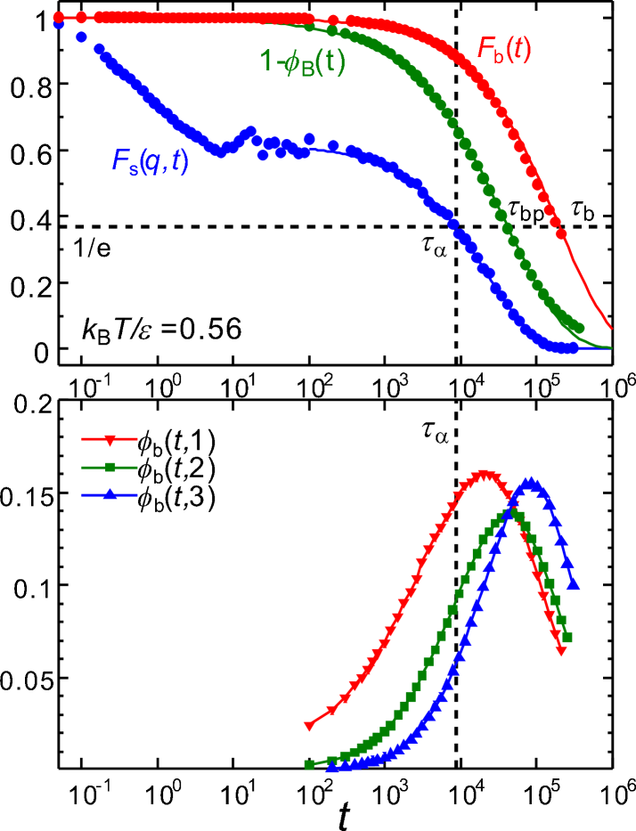
Figure 1: Top: Bond relaxation function Fb​(t)subscript𝐹𝑏𝑑F_{b}(t) in Eq.(3.3), self part of density time-correlation function Fs​(q,t)subscriptπΉπ‘ π‘žπ‘‘F_{s}(q,t) at q=2β€‹Ο€π‘ž2πœ‹q=2\pi in Eq.(3.5), and fraction of non-𝑩𝑩B particles 1βˆ’Ο•b​(t)=Ο•B​(t,0)1subscriptitalic-ϕ𝑏𝑑subscriptitalic-ϕ𝐡𝑑01-\phi_{b}(t)=\phi_{B}(t,0) in Eq.(3.15) at T=0.56𝑇0.56T=0.56 for N=4000𝑁4000N=4000 in 2D. Relaxation times here are τα=8400subscriptπœπ›Ό8400\tau_{\alpha}=8400 from Eq.(3.6), Ο„b=2.0Γ—105β‰…35​ταsubscriptπœπ‘2.0superscript10535subscriptπœπ›Ό\tau_{b}=2.0\times 10^{5}\cong 35\tau_{\alpha} from Eq.(3.4). and Ο„b​p=4.18Γ—104β‰…5​ταsubscriptπœπ‘π‘4.18superscript1045subscriptπœπ›Ό\tau_{bp}=4.18\times 10^{4}\cong 5\tau_{\alpha} from Eq.(3.16). Bottom: fractions of 𝑩𝑩B particles with kπ‘˜k broken bonds Ο•B​(t,k)subscriptitalic-Ο•π΅π‘‘π‘˜\phi_{B}(t,k) in Eq.(3.14) for k=1,2,π‘˜12k=1,2, and 3.
Refer to caption
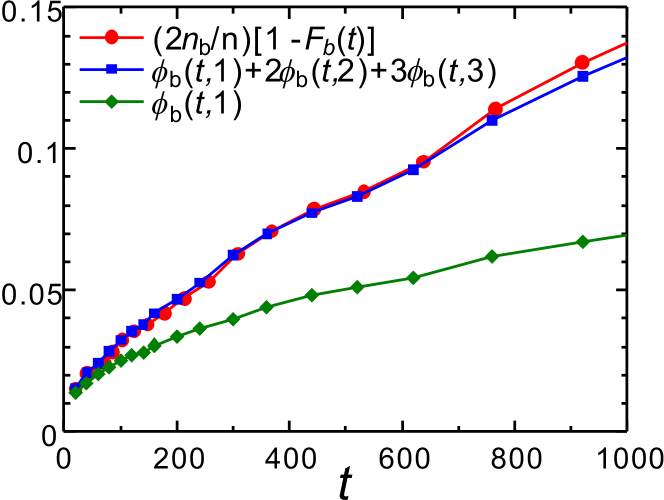
Figure 2: Numerical results of (2​nb/n)​[1βˆ’Fb​(t)]2subscript𝑛𝑏𝑛delimited-[]1subscript𝐹𝑏𝑑(2n_{b}/n)[1-F_{b}(t)], Ο•B​(t,1)subscriptitalic-ϕ𝐡𝑑1\phi_{B}(t,1), and Ο•B​(t,1)+2​ϕB​(t,2)+3​ϕB​(t,3)subscriptitalic-ϕ𝐡𝑑12subscriptitalic-ϕ𝐡𝑑23subscriptitalic-ϕ𝐡𝑑3\phi_{B}(t,1)+2\phi_{B}(t,2)+3\phi_{B}(t,3) as functions of t𝑑t in the early stage at T=0.56𝑇0.56T=0.56 for N=4000𝑁4000N=4000, which confirm Eq.(3.18).

III.1 Background

We regard two particles i𝑖i and j𝑗j with positions 𝒓i​(t)subscript𝒓𝑖𝑑{\mbox{\boldmath$r$}}_{i}(t) and 𝒓j​(t)subscript𝒓𝑗𝑑{\mbox{\boldmath$r$}}_{j}(t) to be bonded if yo ; yo1

ri​j​(t)<A1​σα​β,subscriptπ‘Ÿπ‘–π‘—π‘‘subscript𝐴1subscriptπœŽπ›Όπ›½r_{ij}(t)<A_{1}\sigma_{\alpha\beta}, (3.1)

where iβˆˆΞ±π‘–π›Όi\in\alpha and jβˆˆΞ²π‘—π›½j\in\beta. Hereafter ri​j​(t)=|𝒓i​(t)βˆ’π’“j​(t)|subscriptπ‘Ÿπ‘–π‘—π‘‘subscript𝒓𝑖𝑑subscript𝒓𝑗𝑑r_{ij}(t)=|{\mbox{\boldmath$r$}}_{i}(t)-{\mbox{\boldmath$r$}}_{j}(t)| is the distance between these particles at time t𝑑t. At a later time t+Δ​t𝑑Δ𝑑t+\Delta t, this bond is treated to be broken if

ri​j​(t+Δ​t)>A2​σα​β.subscriptπ‘Ÿπ‘–π‘—π‘‘Ξ”π‘‘subscript𝐴2subscriptπœŽπ›Όπ›½r_{ij}(t+\Delta t)>A_{2}\sigma_{\alpha\beta}. (3.2)

We assume that A1​σα​βsubscript𝐴1subscriptπœŽπ›Όπ›½A_{1}\sigma_{\alpha\beta} is slightly larger than the peak distance of the pair correlation functions gα​β​(r)subscriptπ‘”π›Όπ›½π‘Ÿg_{\alpha\beta}(r) and A2subscript𝐴2A_{2} is somewhat larger than A1subscript𝐴1A_{1}. In this paper, we set A1=1.15subscript𝐴11.15A_{1}=1.15 and A2=1.5subscript𝐴21.5A_{2}=1.5 in 2D and A1=1.3subscript𝐴11.3A_{1}=1.3 and A2=1.7subscript𝐴21.7A_{2}=1.7 in 3D.

Let us consider the bonds at t=t0𝑑subscript𝑑0t=t_{0} and denote their total number as Nb​(t0)subscript𝑁𝑏subscript𝑑0N_{b}(t_{0}). A fraction of them will be broken subsequently and the total number of the remaining bonds Nb​(t0+Δ​t)subscript𝑁𝑏subscript𝑑0Δ𝑑N_{b}(t_{0}+\Delta t) at t=t0+Δ​t𝑑subscript𝑑0Δ𝑑t=t_{0}+\Delta t decays as

Nb​(t0+Δ​t)/Nb​(t0)=Fb​(Δ​t).subscript𝑁𝑏subscript𝑑0Δ𝑑subscript𝑁𝑏subscript𝑑0subscript𝐹𝑏Δ𝑑N_{b}(t_{0}+\Delta t)/N_{b}(t_{0})=F_{b}(\Delta t). (3.3)

For large systems, the relaxation function Fb​(Δ​t)subscript𝐹𝑏Δ𝑑F_{b}(\Delta t) may be treated to depend only on the time difference Δ​tΔ𝑑\Delta t (being nearly independent of the initial time t0subscript𝑑0t_{0} for large N𝑁N). It decreases with increasing Δ​tΔ𝑑\Delta t, so the bond-breakage time Ο„bsubscriptπœπ‘\tau_{b} may be defined by

Fb​(Ο„b)=eβˆ’1.subscript𝐹𝑏subscriptπœπ‘superscript𝑒1F_{b}(\tau_{b})=e^{-1}. (3.4)

On the other hand, the self part of the density time-correlation function is expressed as

Fs​(q,t)=1Nβ€‹βŸ¨βˆ‘jexp⁑[i​𝒒⋅Δ​𝒓j​(t0,t0+t)]⟩.subscriptπΉπ‘ π‘žπ‘‘1𝑁delimited-⟨⟩subscript𝑗⋅𝑖𝒒Δsubscript𝒓𝑗subscript𝑑0subscript𝑑0𝑑F_{s}(q,t)=\frac{1}{N}{\bigg{\langle}}{\sum_{j}\exp[i{\mbox{\boldmath$q$}}\cdot\Delta{\mbox{\boldmath$r$}}_{j}(t_{0},t_{0}+t)]}{\bigg{\rangle}}. (3.5)

where Δ​𝒓j​(t0,t1)=𝒓j​(t1)βˆ’π’“j​(t0)Ξ”subscript𝒓𝑗subscript𝑑0subscript𝑑1subscript𝒓𝑗subscript𝑑1subscript𝒓𝑗subscript𝑑0\Delta{\mbox{\boldmath$r$}}_{j}(t_{0},t_{1})={\mbox{\boldmath$r$}}_{j}(t_{1})-{\mbox{\boldmath$r$}}_{j}(t_{0}) is the displacement vector of particle j𝑗j and 𝒒𝒒q is the wave vector. In Eq.(3.5), the average is taken over all the particles. In our simulation, the average over the initial time t0subscript𝑑0t_{0} and that over a number of runs were also taken. The structural relaxation time ταsubscriptπœπ›Ό\tau_{\alpha} is usually defined at q=2β€‹Ο€π‘ž2πœ‹q=2\pi by

Fs​(q,τα)=eβˆ’1.subscriptπΉπ‘ π‘žsubscriptπœπ›Όsuperscript𝑒1F_{s}(q,\tau_{\alpha})=e^{-1}. (3.6)

Wave numbers will be measured in units of Οƒ1βˆ’1superscriptsubscript𝜎11\sigma_{1}^{-1}.

In the upper panel of Fig.1, we display Fb​(t)subscript𝐹𝑏𝑑F_{b}(t) and Fs​(q,t)subscriptπΉπ‘ π‘žπ‘‘F_{s}(q,t) at q=2β€‹Ο€π‘ž2πœ‹q=2\pi for T=0.56𝑇0.56T=0.56 and N=4000𝑁4000N=4000, where τα=8.4Γ—103subscriptπœπ›Ό8.4superscript103\tau_{\alpha}=8.4\times 10^{3} and Ο„b=2.0Γ—105β‰…35​ταsubscriptπœπ‘2.0superscript10535subscriptπœπ›Ό\tau_{b}=2.0\times 10^{5}\cong 35\tau_{\alpha}. In the previous paper yo1 , the relation Ο„bβ‰…10​ταsubscriptπœπ‘10subscriptπœπ›Ό\tau_{b}\cong 10\tau_{\alpha} was found for binary mixtures with the soft-core potentential wih N=104𝑁superscript104N=10^{4} in 3D. Both in 2D and 3D, Fb​(t)subscript𝐹𝑏𝑑F_{b}(t) may fairly be fitted to the stretched exponential form at low T𝑇T as

Fb​(t)β‰…exp⁑[βˆ’(t/Ο„b)c],subscript𝐹𝑏𝑑superscript𝑑subscriptπœπ‘π‘F_{b}(t)\cong\exp[-(t/\tau_{b})^{c}], (3.7)

in the range t≲τbless-than-or-similar-to𝑑subscriptπœπ‘t\lesssim\tau_{b}. At T=0.56𝑇0.56T=0.56 we obtain c∼0.58similar-to𝑐0.58c\sim 0.58 in 2D. The exponent c𝑐c increases with decreasing T𝑇T. In contrast, Fs​(q,t)subscriptπΉπ‘ π‘žπ‘‘F_{s}(q,t) exhibits a plateau fp(<1)annotatedsubscript𝑓pabsent1f_{\rm p}(<1) before the α𝛼\alpha relaxation at low T𝑇T due to the thermal vibrational motions (see the appendix).

III.2 Bond-breakage correlations

Here, we present a generalized formulation of the bond breakage to introduce broken-bond correlation functions. To this end, we define two overlap functions wα​β(1)​(r)superscriptsubscript𝑀𝛼𝛽1π‘Ÿw_{\alpha\beta}^{(1)}({r}) and wα​β(2)​(r)superscriptsubscript𝑀𝛼𝛽2π‘Ÿw_{\alpha\beta}^{(2)}({r}) depending on the particle distance rπ‘Ÿr as

wα​β(K)​(r)=θ​(AKβ€‹ΟƒΞ±β€‹Ξ²βˆ’r),superscriptsubscriptπ‘€π›Όπ›½πΎπ‘Ÿπœƒsubscript𝐴𝐾subscriptπœŽπ›Όπ›½π‘Ÿw_{\alpha\beta}^{(K)}(r)=\theta(A_{K}\sigma_{\alpha\beta}-r), (3.8)

with A1subscript𝐴1A_{1} and A2subscript𝐴2A_{2} being defined in Eqs.(3.1) and (3.2). The θ​(u)πœƒπ‘’\theta(u) is the step function being equal to 1 for u>0𝑒0u>0 and to 0 for u≀0𝑒0u\leq 0. The fluctuating number density of the bonds may then be defined as

n^b​(𝒓,t)=12β€‹βˆ‘i​jwα​β(1)​(ri​j​(t))​δ​(π’“βˆ’π’“i​(t)),subscript^𝑛𝑏𝒓𝑑12subscript𝑖𝑗superscriptsubscript𝑀𝛼𝛽1subscriptπ‘Ÿπ‘–π‘—π‘‘π›Ώπ’“subscript𝒓𝑖𝑑\hat{n}_{b}({\mbox{\boldmath$r$}},t)=\frac{1}{2}\sum_{ij}w_{\alpha\beta}^{(1)}(r_{ij}(t))\delta({\mbox{\boldmath$r$}}-{\mbox{\boldmath$r$}}_{i}(t)), (3.9)

where we multiply 1/2121/2 because a bond is supported by two particles in our definition. The statistical average of n^b​(𝒓,t)subscript^𝑛𝑏𝒓𝑑\hat{n}_{b}({\mbox{\boldmath$r$}},t) is the average bond number density,

nb=1Vβ€‹βˆ«π‘‘π’“β€‹n^b​(𝒓,t)=1V​Nb​(0).subscript𝑛𝑏1𝑉differential-d𝒓subscript^𝑛𝑏𝒓𝑑1𝑉subscript𝑁𝑏0n_{b}=\frac{1}{V}\int{d{\mbox{\boldmath$r$}}}{\hat{n}_{b}({\mbox{\boldmath$r$}},t)}=\frac{1}{V}N_{b}(0). (3.10)

Here, nb∼3​nsimilar-tosubscript𝑛𝑏3𝑛n_{b}\sim 3n in 2D at high densities. In fact, we numerically obtain nb=2.28=2.81​nsubscript𝑛𝑏2.282.81𝑛n_{b}=2.28=2.81n for n=0.811𝑛0.811n=0.811 in our 2D system. Now we may introduce the broken bond number density in time interval [t0,t1]subscript𝑑0subscript𝑑1[t_{0},t_{1}] as

𝒫^​(𝒓,t0,t1)=12β€‹βˆ‘iℬi​(t0,t1)​δ​(π’“βˆ’π’“i​(t0)),^𝒫𝒓subscript𝑑0subscript𝑑112subscript𝑖subscriptℬ𝑖subscript𝑑0subscript𝑑1𝛿𝒓subscript𝒓𝑖subscript𝑑0\hat{\cal P}({\mbox{\boldmath$r$}},t_{0},t_{1})=\frac{1}{2}\sum_{i}{\cal B}_{i}(t_{0},t_{1})\delta({\mbox{\boldmath$r$}}-{\mbox{\boldmath$r$}}_{i}(t_{0})), (3.11)

where ℬi​(t0,t1)subscriptℬ𝑖subscript𝑑0subscript𝑑1{\cal B}_{i}(t_{0},t_{1}) is the broken bond number of particle i𝑖i assuming a nonnegative integer quantity as

ℬi​(t0,t1)=βˆ‘jwα​β(1)​(ri​j​(t0))​[1βˆ’wα​β(2)​(ri​j​(t1))].subscriptℬ𝑖subscript𝑑0subscript𝑑1subscript𝑗superscriptsubscript𝑀𝛼𝛽1subscriptπ‘Ÿπ‘–π‘—subscript𝑑0delimited-[]1superscriptsubscript𝑀𝛼𝛽2subscriptπ‘Ÿπ‘–π‘—subscript𝑑1{\cal B}_{i}(t_{0},t_{1})=\sum_{j}w_{\alpha\beta}^{(1)}(r_{ij}(t_{0}))[1-w_{\alpha\beta}^{(2)}({r}_{ij}(t_{1}))]. (3.12)

This number tends to zero as t1β†’t0β†’subscript𝑑1subscript𝑑0t_{1}\to t_{0} from A1<A2subscript𝐴1subscript𝐴2A_{1}<A_{2} and increases to 1,2,β‹―12β‹―1,2,\cdots upon bond breakage. Hereafter, the particles with ℬi​(t0,t1)β‰₯1subscriptℬ𝑖subscript𝑑0subscript𝑑11{\cal B}_{i}(t_{0},t_{1})\geq 1 are called 𝑩𝑩B particles, which are surrounded by different particle configurations at the initial and final times t=t0𝑑subscript𝑑0t=t_{0} and t1subscript𝑑1t_{1}. On the other hand, those with ℬi​(t0,t1)=0subscriptℬ𝑖subscript𝑑0subscript𝑑10{\cal B}_{i}(t_{0},t_{1})=0 are called non-𝑩𝑩B particles, which have the same surrounding configurations at t=t0𝑑subscript𝑑0t=t_{0} and t1subscript𝑑1t_{1}. The statistical average βŸ¨π’«^​(𝒓,t0,t1)⟩delimited-⟨⟩^𝒫𝒓subscript𝑑0subscript𝑑1\langle{\hat{\cal P}({\mbox{\boldmath$r$}},t_{0},t_{1})}\rangle depends on the time difference t=t1βˆ’t0𝑑subscript𝑑1subscript𝑑0t=t_{1}-t_{0} as

pb​(t)=1Vβ€‹βˆ«π‘‘π’“β€‹π’«^​(𝒓,t0,t1)=nb​[1βˆ’Fb​(t)]subscript𝑝𝑏𝑑1𝑉differential-d𝒓^𝒫𝒓subscript𝑑0subscript𝑑1subscript𝑛𝑏delimited-[]1subscript𝐹𝑏𝑑p_{b}(t)=\frac{1}{V}\int{d{\mbox{\boldmath$r$}}}{\hat{\cal P}({\mbox{\boldmath$r$}},t_{0},t_{1})}=n_{b}[1-F_{b}(t)] (3.13)

where nbsubscript𝑛𝑏n_{b} is defined by Eq.(3.10) and Fb​(t)subscript𝐹𝑏𝑑F_{b}(t) by Eq.(3.6).

Let the number of the particles with ℬi​(t0,t1)=ksubscriptℬ𝑖subscript𝑑0subscript𝑑1π‘˜{\cal B}_{i}(t_{0},t_{1})=k be NB​(t,k)subscriptπ‘π΅π‘‘π‘˜N_{B}(t,k) (k=0,1,β‹―π‘˜01β‹―k=0,1,\cdots) with t=t1βˆ’t0𝑑subscript𝑑1subscript𝑑0t=t_{1}-t_{0}. Then,

Ο•B​(t,k)=NB​(t,k)/Nsubscriptitalic-Ο•π΅π‘‘π‘˜subscriptπ‘π΅π‘‘π‘˜π‘\phi_{B}(t,k)=N_{B}(t,k)/N (3.14)

is the fraction of the 𝑩𝑩B particles with kπ‘˜k broken bonds for kβ‰₯1π‘˜1k\geq 1, while Ο•B​(t,0)=NB​(t,0)/Nsubscriptitalic-ϕ𝐡𝑑0subscript𝑁𝐡𝑑0𝑁\phi_{B}(t,0)=N_{B}(t,0)/N is the fraction of the non-𝑩𝑩B particles. The fraction of the total 𝑩𝑩B particles is the following sum,

Ο•b​(t)=βˆ‘kβ‰₯1Ο•B​(t,k)=1βˆ’Ο•B​(t,0).subscriptitalic-ϕ𝑏𝑑subscriptπ‘˜1subscriptitalic-Ο•π΅π‘‘π‘˜1subscriptitalic-ϕ𝐡𝑑0\phi_{b}(t)=\sum_{k\geq 1}\phi_{B}(t,k)=1-\phi_{B}(t,0). (3.15)

We define the bond-preserving time Ο„b​psubscriptπœπ‘π‘\tau_{bp} as

1βˆ’Ο•b​(Ο„b​p)=Ο•B​(Ο„b​p,0)=eβˆ’1.1subscriptitalic-ϕ𝑏subscriptπœπ‘π‘subscriptitalic-ϕ𝐡subscriptπœπ‘π‘0superscript𝑒11-\phi_{b}(\tau_{bp})=\phi_{B}(\tau_{bp},0)=e^{-1}. (3.16)

The particles have a broken bond on this time scale. Since each particle has several bonds (∼6similar-toabsent6\sim 6 in 2D), Ο„b​psubscriptπœπ‘π‘\tau_{bp} is considerably shorter than the bond breakage time Ο„bsubscriptπœπ‘\tau_{b} in Eq.(3.4). For t≳τb​pgreater-than-or-equivalent-to𝑑subscriptπœπ‘π‘t\gtrsim\tau_{bp}, the structural relaxation becomes appreciable. From Eq.(3.14) we obtain

pb​(t)=n2β€‹βˆ‘kk​ϕb​(t,k)subscript𝑝𝑏𝑑𝑛2subscriptπ‘˜π‘˜subscriptitalic-Ο•π‘π‘‘π‘˜p_{b}(t)=\frac{n}{2}\sum_{k}k\phi_{b}(t,k) (3.17)

From Eqs.(3.13) and (3.17) we find

2​nbn​[1βˆ’Fb​(t)]=βˆ‘kk​ϕb​(t,k)2subscript𝑛𝑏𝑛delimited-[]1subscript𝐹𝑏𝑑subscriptπ‘˜π‘˜subscriptitalic-Ο•π‘π‘‘π‘˜2\frac{n_{b}}{n}[1-F_{b}(t)]=\sum_{k}k\phi_{b}(t,k) (3.18)

Setting t=t1βˆ’t0𝑑subscript𝑑1subscript𝑑0t=t_{1}-t_{0} in steady states, we introduce the bond-breakage space-time correlation function,

Gb​(r,t)subscriptπΊπ‘π‘Ÿπ‘‘\displaystyle G_{b}({r},t) =\displaystyle= βŸ¨π’«^​(𝒓+𝒓′,t0,t1)​𝒫^​(𝒓′,t0,t1)⟩delimited-⟨⟩^𝒫𝒓superscript𝒓′subscript𝑑0subscript𝑑1^𝒫superscript𝒓′subscript𝑑0subscript𝑑1\displaystyle\langle{\hat{\cal{P}}({\mbox{\boldmath$r$}}+{\mbox{\boldmath$r$}}^{\prime},t_{0},t_{1})\hat{\cal{P}}({\mbox{\boldmath$r$}}^{\prime},t_{0},t_{1})}\rangle (3.19)
=14​Vβ€‹βŸ¨βˆ‘i​kℬi​(t0,t1)​ℬk​(t0,t1)​δ​(π’“βˆ’π’“i​k​(t0))⟩,absent14𝑉delimited-⟨⟩subscriptπ‘–π‘˜subscriptℬ𝑖subscript𝑑0subscript𝑑1subscriptβ„¬π‘˜subscript𝑑0subscript𝑑1𝛿𝒓subscriptπ’“π‘–π‘˜subscript𝑑0\displaystyle=\frac{1}{4V}{\bigg{\langle}}{\sum_{ik}{\cal B}_{i}(t_{0},t_{1}){\cal B}_{k}(t_{0},t_{1})\delta({\mbox{\boldmath$r$}}-{\mbox{\boldmath$r$}}_{ik}(t_{0}))}{\bigg{\rangle}},

where 𝒓i​k​(t0)=𝒓i​(t0)βˆ’π’“k​(t0)subscriptπ’“π‘–π‘˜subscript𝑑0subscript𝒓𝑖subscript𝑑0subscriptπ’“π‘˜subscript𝑑0{\mbox{\boldmath$r$}}_{ik}(t_{0})={\mbox{\boldmath$r$}}_{i}(t_{0})-{\mbox{\boldmath$r$}}_{k}(t_{0}). From Eq.(3.13) we have Gb​(r,t)β†’pb​(t)2β†’subscriptπΊπ‘π‘Ÿπ‘‘subscript𝑝𝑏superscript𝑑2G_{b}(r,t)\to p_{b}(t)^{2} for large rπ‘Ÿr. The structure factor of the broken bonds is given by

Sb​(q,t)subscriptπ‘†π‘π‘žπ‘‘\displaystyle S_{b}(q,t) =\displaystyle= 1Vβ€‹βŸ¨|𝒫^𝒒​(t0,t1)|2⟩1𝑉delimited-⟨⟩superscriptsubscript^𝒫𝒒subscript𝑑0subscript𝑑12\displaystyle\frac{1}{V}\langle{|\hat{\cal P}_{\mbox{\boldmath$q$}}(t_{0},t_{1})|^{2}}\rangle (3.20)
=βˆ«π‘‘π’“β€‹[Gb​(𝒓,t)βˆ’pb​(t)2]​ei​𝒒⋅𝒓,absentdifferential-d𝒓delimited-[]subscript𝐺𝑏𝒓𝑑subscript𝑝𝑏superscript𝑑2superscript𝑒⋅𝑖𝒒𝒓\displaystyle=\int d{\mbox{\boldmath$r$}}[G_{b}({\mbox{\boldmath$r$}},t)-p_{b}(t)^{2}]e^{i{\mbox{\boldmath$q$}}\cdot{\mbox{\boldmath$r$}}},

where 𝒒𝒒q is the wave vector, q=|𝒒|π‘žπ’’q=|{\mbox{\boldmath$q$}}| is the wave number, and 𝒫^𝒒​(t0,t1)=βˆ‘jℬj​(t0,t1)​exp⁑[i​𝒒⋅𝒓i​(t0)]/2subscript^𝒫𝒒subscript𝑑0subscript𝑑1subscript𝑗subscriptℬ𝑗subscript𝑑0subscript𝑑1⋅𝑖𝒒subscript𝒓𝑖subscript𝑑02{\hat{\cal P}}_{\mbox{\boldmath$q$}}(t_{0},t_{1})=\sum_{j}{\cal B}_{j}(t_{0},t_{1})\exp[i{\mbox{\boldmath$q$}}\cdot{\mbox{\boldmath$r$}}_{i}(t_{0})]/2 is the Fourier component of 𝒫^​(𝒓,t0,t1)^𝒫𝒓subscript𝑑0subscript𝑑1{\hat{\cal P}}({\mbox{\boldmath$r$}},t_{0},t_{1}).

As in the four-point scheme Lacevic , we introduce the susceptibility Ο‡b​(t)subscriptπœ’π‘π‘‘\chi_{b}(t) to represent the overall degree of the bond-breakage correlations as follows:

Ο‡b​(t)=14​Vβ€‹βŸ¨βˆ‘i​kδ​ℬi​(t0,t1)​δ​ℬk​(t0,t1)⟩,subscriptπœ’π‘π‘‘14𝑉delimited-⟨⟩subscriptπ‘–π‘˜π›Ώsubscriptℬ𝑖subscript𝑑0subscript𝑑1𝛿subscriptβ„¬π‘˜subscript𝑑0subscript𝑑1\chi_{b}(t)=\frac{1}{4V}{\bigg{\langle}}{\sum_{ik}\delta{\cal B}_{i}(t_{0},t_{1})\delta{\cal B}_{k}(t_{0},t_{1})}{\bigg{\rangle}}, (3.21)

in terms of the deviations δ​ℬi​(t0,t1)=ℬi​(t0,t1)βˆ’2​pb​(t)/n𝛿subscriptℬ𝑖subscript𝑑0subscript𝑑1subscriptℬ𝑖subscript𝑑0subscript𝑑12subscript𝑝𝑏𝑑𝑛\delta{\cal B}_{i}(t_{0},t_{1})={\cal B}_{i}(t_{0},t_{1})-2p_{b}(t)/n. Here βŸ¨β„¬i⟩=βˆ‘iℬi/N=2​pb/ndelimited-⟨⟩subscriptℬ𝑖subscript𝑖subscriptℬ𝑖𝑁2subscript𝑝𝑏𝑛\langle{{\cal B}_{i}}\rangle=\sum_{i}{\cal B}_{i}/N=2p_{b}/n from Eqs.(3.11) and (3.13). In Sb​(q,t)subscriptπ‘†π‘π‘žπ‘‘S_{b}(q,t) and Ο‡b​(t)subscriptπœ’π‘π‘‘\chi_{b}(t), the four particle positions 𝒓i​(t0)subscript𝒓𝑖subscript𝑑0{\mbox{\boldmath$r$}}_{i}(t_{0}), 𝒓k​(t0)subscriptπ’“π‘˜subscript𝑑0{\mbox{\boldmath$r$}}_{k}(t_{0}), 𝒓j​(t1)subscript𝒓𝑗subscript𝑑1{\mbox{\boldmath$r$}}_{j}(t_{1}), and 𝒓ℓ​(t1)subscript𝒓ℓsubscript𝑑1{\mbox{\boldmath$r$}}_{\ell}(t_{1}) are involved. In this sense, they are four-point correlation functions.

Rabini et al. Rabini introduced the number of particles that have left particle i𝑖i’s original neighbors at time t𝑑t. It involves two times and was written as niout​(0,t)superscriptsubscript𝑛𝑖out0𝑑n_{i}^{\rm out}(0,t). It is similar to our ℬi​(t0,t0+t)subscriptℬ𝑖subscript𝑑0subscript𝑑0𝑑{\cal B}_{i}(t_{0},t_{0}+t) in Eq.(3.12). Abate and Durian Durian introduced a bond-breakage susceptibility Ο‡B​(t)subscriptπœ’π΅π‘‘\chi_{B}(t) similar to ours in Eq.(3.21) for a quasi-two-dimensional granular system of air-fluidized beads.
Refer to caption
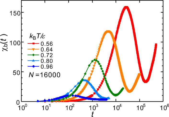
Figure 3: Susceptibility Ο‡b​(t)subscriptπœ’π‘π‘‘\chi_{b}(t) in Eq.(3.21) vs t𝑑t exhibiting a peak at t=tbmax𝑑superscriptsubscript𝑑𝑏maxt=t_{b}^{\rm max} for N=16000𝑁16000N=16000.
Refer to caption
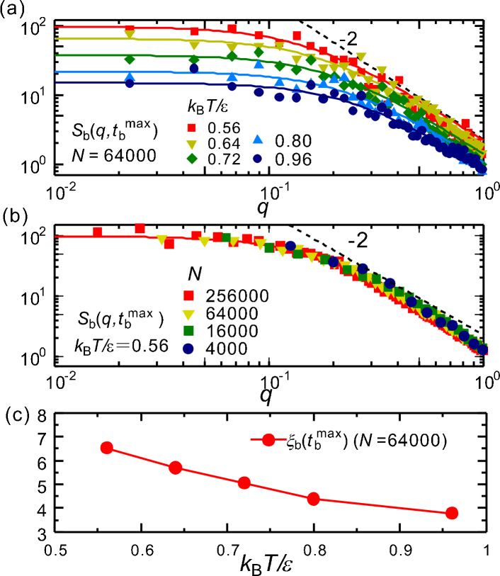
Figure 4: (a) Structure factor Sb​(q,tbmax)subscriptπ‘†π‘π‘žsuperscriptsubscript𝑑𝑏maxS_{b}(q,t_{b}^{\rm max}) for bond breakage in Eq.(3.20) at various T𝑇T for N=64000𝑁64000N=64000, (b) Sb​(q,tbmax)subscriptπ‘†π‘π‘žsuperscriptsubscript𝑑𝑏maxS_{b}(q,t_{b}^{\rm max}) at T=0.56𝑇0.56T=0.56 for various N𝑁N, and (c) correlation lengths ΞΎb=ΞΎb​(tbmax)subscriptπœ‰π‘subscriptπœ‰π‘superscriptsubscript𝑑𝑏max\xi_{b}=\xi_{b}(t_{b}^{\rm max}) vs T𝑇T for N=64000𝑁64000N=64000. Sb​(q,t)subscriptπ‘†π‘π‘žπ‘‘S_{b}(q,t) is approximately on a single curve independent of N𝑁N, leading to weak system-size dependence of ΞΎbsubscriptπœ‰π‘\xi_{b} for 1β‰ͺΞΎbβ‰ͺLmuch-less-than1subscriptπœ‰π‘much-less-than𝐿1\ll\xi_{b}\ll L.

III.3 Numerical results on bond breakage

We further discuss consequences of our theory using numerical results in 2D. In Fig.1, we plot 1βˆ’Ο•b​(t)=Ο•B​(t,0)1subscriptitalic-ϕ𝑏𝑑subscriptitalic-ϕ𝐡𝑑01-\phi_{b}(t)=\phi_{B}(t,0) in the upper panel and Ο•B​(t,k)subscriptitalic-Ο•π΅π‘‘π‘˜\phi_{B}(t,k) with k=1,2π‘˜12k=1,2, and 3 in the lower panel, where Ο„b​p=41800β‰…5​τα=0.14​τbsubscriptπœπ‘π‘418005subscriptπœπ›Ό0.14subscriptπœπ‘\tau_{bp}=41800\cong 5\tau_{\alpha}=0.14\tau_{b} from Eq.(3.16). At small t𝑑t, Ο•B​(t,k)subscriptitalic-Ο•π΅π‘‘π‘˜\phi_{B}(t,k) grow as

Ο•B​(t,k)∝tak,proportional-tosubscriptitalic-Ο•π΅π‘‘π‘˜superscript𝑑subscriptπ‘Žπ‘˜{\phi}_{B}(t,k)\propto t^{a_{k}}, (3.22)

where a1∼0.60similar-tosubscriptπ‘Ž10.60a_{1}\sim 0.60, a2∼1.0similar-tosubscriptπ‘Ž21.0a_{2}\sim 1.0, and a3∼1.3similar-tosubscriptπ‘Ž31.3a_{3}\sim 1.3. Though we cannot derive these exponents theoretically, they should arise from correlated occurrence of bond breakage events.

In Fig.2, we confirm the validity of Eq.(3.18) from simulation at T=0.56𝑇0.56T=0.56, where nb/n=3.17subscript𝑛𝑏𝑛3.17n_{b}/n=3.17. We find that (2​nb/n)​[1βˆ’Fb​(t)]2subscript𝑛𝑏𝑛delimited-[]1subscript𝐹𝑏𝑑(2n_{b}/n)[1-F_{b}(t)] nearly coincides with Ο•B​(t,1)subscriptitalic-ϕ𝐡𝑑1\phi_{B}(t,1) for t<200𝑑200t<200 and with Ο•B​(t,1)+2​ϕB​(t,2)+3​ϕB​(t,3)subscriptitalic-ϕ𝐡𝑑12subscriptitalic-ϕ𝐡𝑑23subscriptitalic-ϕ𝐡𝑑3\phi_{B}(t,1)+2\phi_{B}(t,2)+3\phi_{B}(t,3) for t<4000𝑑4000t<4000 within a few %percent\% differences. The first relation for k=1π‘˜1k=1 in Eq.(3.22) is consistent with Eq.(3.18) since a1β‰…csubscriptπ‘Ž1𝑐a_{1}\cong c. In fact, for tβ‰ͺΟ„bmuch-less-than𝑑subscriptπœπ‘t\ll\tau_{b}, Eqs.(3.7) and (3.18) yield

Ο•B​(t,1)β‰…(2​nb/n)​(t/Ο„b)c.subscriptitalic-ϕ𝐡𝑑12subscript𝑛𝑏𝑛superscript𝑑subscriptπœπ‘π‘\phi_{B}(t,1)\cong(2{n_{b}}/{n})(t/\tau_{b})^{c}. (3.23)

In Fig.3, we plot Ο‡b​(t)subscriptπœ’π‘π‘‘\chi_{b}(t) in Eq.(3.21) as a function of t𝑑t for N=16000𝑁16000N=16000, which exhibits a peak at t=tbmax𝑑superscriptsubscript𝑑𝑏maxt=t_{b}^{\rm max}. Here, we have Ο•b​(t)∼0.5similar-tosubscriptitalic-ϕ𝑏𝑑0.5\phi_{b}(t)\sim 0.5 at t=tbmax𝑑superscriptsubscript𝑑𝑏maxt=t_{b}^{\rm max}, which can be seen in Fig.1 for N=4000𝑁4000N=4000 and T=0.56𝑇0.56T=0.56. Here, however, Ο‡b​(t)subscriptπœ’π‘π‘‘\chi_{b}(t) begins to increase for t>tbmax𝑑superscriptsubscript𝑑𝑏maxt>t_{b}^{\rm max}, because the 𝑩𝑩B particles with ℬi=2,3,β‹―subscriptℬ𝑖23β‹―{\cal B}_{i}=2,3,\cdots becomes appreaciable at very long times (see Fig.1). In (a) of Fig.4, we show Sb​(q,tbmax)subscriptπ‘†π‘π‘žsuperscriptsubscript𝑑𝑏maxS_{b}(q,t_{b}^{\rm max}) vs qπ‘žq for various T𝑇T with N=64000𝑁64000N=64000. In its calculation we took the average over the initial time t0subscript𝑑0t_{0} in a wide range of [0,106]0superscript106[0,10^{6}] for Tβ‰₯0.64𝑇0.64T\geq 0.64 and that of [0,2Γ—106]02superscript106[0,2\times 10^{6}] for T=0.56𝑇0.56T=0.56, which was needed because of the slow bond breakage. We may fairly fit Sb​(q,t)subscriptπ‘†π‘π‘žπ‘‘S_{b}(q,t) to the Ornstein-Zernike form yo ; yo1 ,

Sb​(q,t)=Ο‡b0​(t)/[1+q2​ξb​(t)2],subscriptπ‘†π‘π‘žπ‘‘superscriptsubscriptπœ’π‘0𝑑delimited-[]1superscriptπ‘ž2subscriptπœ‰π‘superscript𝑑2S_{b}(q,t)=\chi_{b}^{0}(t)/[1+q^{2}\xi_{b}(t)^{2}], (3.24)

where Ο‡b0​(t)=limqβ†’0Sb​(q,t)superscriptsubscriptπœ’π‘0𝑑subscriptβ†’π‘ž0subscriptπ‘†π‘π‘žπ‘‘\chi_{b}^{0}(t)=\lim_{q\to 0}S_{b}(q,t) is the long wavelength limit of Sb​(q,t)subscriptπ‘†π‘π‘žπ‘‘S_{b}(q,t) and ΞΎb=ΞΎb​(t)subscriptπœ‰π‘subscriptπœ‰π‘π‘‘\xi_{b}=\xi_{b}(t) is the correlation length representing the spatial scale of the correlated configuration changes. Furthermore, in (b), we show Sb​(q,tbmax)subscriptπ‘†π‘π‘žsuperscriptsubscript𝑑𝑏maxS_{b}(q,t_{b}^{\rm max}) vs qπ‘žq at T=0.56𝑇0.56T=0.56 for various N𝑁N, which demonstrates weak system-size dependence of the bond-breakage correlations. For N=256000𝑁256000N=256000, however, the averaging over the initial time t0subscript𝑑0t_{0} is still insufficient because of very large tbmax∼4Γ—104similar-tosuperscriptsubscript𝑑𝑏max4superscript104t_{b}^{\rm max}\sim 4\times 10^{4} as compared to the simulation time (∼105similar-toabsentsuperscript105\sim 10^{5}). As a result, the corresponding Sb​(q,tbmax)subscriptπ‘†π‘π‘žsuperscriptsubscript𝑑𝑏maxS_{b}(q,t_{b}^{\rm max}) exhibit noticeable fluctuations at small qπ‘žq. In (c), the correlation length ΞΎbsubscriptπœ‰π‘\xi_{b} vs T𝑇T is plotted at t=tbmax𝑑superscriptsubscript𝑑𝑏maxt=t_{b}^{\rm max} for N=64000𝑁64000N=64000, which increases with lowering T𝑇T. Note that ΞΎb=ΞΎb​(tbmax)subscriptπœ‰π‘subscriptπœ‰π‘superscriptsubscript𝑑𝑏max\xi_{b}=\xi_{b}(t_{b}^{\rm max}) is nearly independent of the system size from (b) as long as 1β‰ͺΞΎbβ‰ͺLmuch-less-than1subscriptπœ‰π‘much-less-than𝐿1\ll\xi_{b}\ll L.

In the original papersyo ; yo1 , the broken-bond structure factor was defined differently, so it is written as SbYO​(q,t)superscriptsubscript𝑆𝑏YOπ‘žπ‘‘S_{b}^{\rm YO}(q,t) here. It was calculated for the Fourier component of the following broken bond number density,

𝒫^YO​(𝒓,t0,t1)=12β€‹βˆ‘i​jwα​β(1)​(ri​j​(t0))​[1βˆ’wα​β(2)​(ri​j​(t1))]subscript^𝒫YO𝒓subscript𝑑0subscript𝑑112subscript𝑖𝑗superscriptsubscript𝑀𝛼𝛽1subscriptπ‘Ÿπ‘–π‘—subscript𝑑0delimited-[]1superscriptsubscript𝑀𝛼𝛽2subscriptπ‘Ÿπ‘–π‘—subscript𝑑1\displaystyle\hat{\cal P}_{\rm YO}({\mbox{\boldmath$r$}},t_{0},t_{1})=\frac{1}{2}\sum_{ij}w_{\alpha\beta}^{(1)}(r_{ij}(t_{0}))[1-w_{\alpha\beta}^{(2)}({r}_{ij}(t_{1}))]
×δ​(π’“βˆ’π‘Ήi​j​(t0)),absent𝛿𝒓subscript𝑹𝑖𝑗subscript𝑑0\displaystyle\times\delta({\mbox{\boldmath$r$}}-{\mbox{\boldmath$R$}}_{ij}(t_{0})), (3.25)

where t=t1βˆ’t0𝑑subscript𝑑1subscript𝑑0t=t_{1}-t_{0} was set equal to 0.05​τb0.05subscriptπœπ‘0.05\tau_{b} or 0.1​τb0.1subscriptπœπ‘0.1\tau_{b}. Here, the midpoint position 𝑹i​j​(t0)=12​(𝒓i​(t0)+𝒓j​(t0))subscript𝑹𝑖𝑗subscript𝑑012subscript𝒓𝑖subscript𝑑0subscript𝒓𝑗subscript𝑑0{\mbox{\boldmath$R$}}_{ij}(t_{0})=\frac{1}{2}({\mbox{\boldmath$r$}}_{i}(t_{0})+{\mbox{\boldmath$r$}}_{j}(t_{0})) of the two particles i𝑖i and j𝑗j is used instead of the position 𝒓i​(t0)subscript𝒓𝑖subscript𝑑0{\mbox{\boldmath$r$}}_{i}(t_{0}) in δ​(π’“βˆ’π’“i​(t0))𝛿𝒓subscript𝒓𝑖subscript𝑑0\delta({\mbox{\boldmath$r$}}-{\mbox{\boldmath$r$}}_{i}(t_{0})) in Eq.(3.11). Note that the particles pairs with a common broken bond are included in Sb​(q,t)subscriptπ‘†π‘π‘žπ‘‘S_{b}(q,t). As a result, the inter-particle peak at qβ‰…2β€‹Ο€π‘ž2πœ‹q\cong 2\pi appears in Sb​(q,t)subscriptπ‘†π‘π‘žπ‘‘S_{b}(q,t) (which is not shown in Fig.4), while it does not apppear in SbYO​(q,t)superscriptsubscript𝑆𝑏YOπ‘žπ‘‘S_{b}^{\rm YO}(q,t). However, there is no essential difference between these two definitions for q<2π‘ž2q<2. In addition, in the previous work yo1 , the dynamic scaling relation of the form Ο„b∼ξbzsimilar-tosubscriptπœπ‘superscriptsubscriptπœ‰π‘π‘§\tau_{b}\sim\xi_{b}^{z} was obtained, where z=4𝑧4z=4 in 2D and z=2𝑧2z=2 in 3D.

IV Four-point theory

Refer to caption
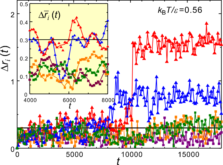
Figure 5: Time evolution of Δ​ri​(t0,t0+t)Ξ”subscriptπ‘Ÿπ‘–subscript𝑑0subscript𝑑0𝑑\Delta r_{i}(t_{0},t_{0}+t) for five particles among 400040004000 particles. They exhibit thermal fluctuations with magnitudes on the order of the overlap length 0.30.30.3. Two particles escape from the initial circle at t∼8000similar-to𝑑8000t\sim 8000 (blue β–³β–³\triangle) and ∼104similar-toabsentsuperscript104\sim 10^{4} (red β–³β–³\triangle). They have a broken bond with ℬi​(t0,t0+t)=1subscriptℬ𝑖subscript𝑑0subscript𝑑0𝑑1{\cal B}_{i}(t_{0},t_{0}+t)=1 and β„±i​(t0,t0+t)=0subscriptℱ𝑖subscript𝑑0subscript𝑑0𝑑0{\cal F}_{i}(t_{0},t_{0}+t)=0 in later times. For the other three particles, the bonds are preserved, but β„±isubscriptℱ𝑖{\cal F}_{i} frequently fluctuate between 1 and 0 in the time range displayed. Inset: Time evolution of the time-smoothed distance Δ​rΒ―i​(t)Ξ”subscriptΒ―π‘Ÿπ‘–π‘‘\Delta{\bar{r}}_{i}(t) defined in Eqs.(4.8) and (4.10) in the range 4000<t<80004000𝑑80004000<t<8000.
Refer to caption
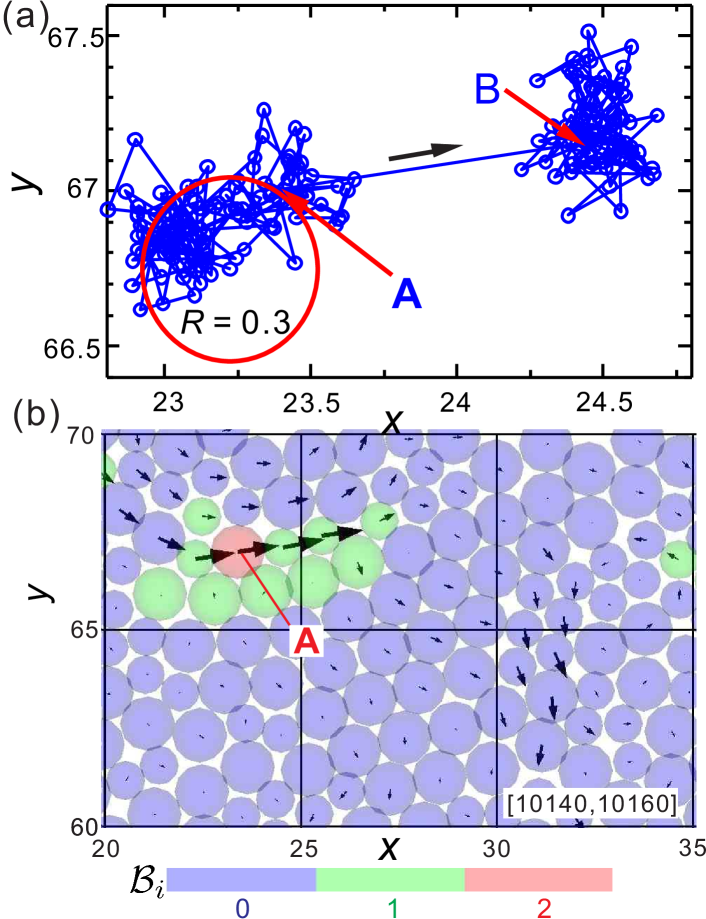
Figure 6: (a) Trajectory of the particle escaping from a cage (red line in Fig.5). Data points at t=8000+20​k𝑑800020π‘˜t=8000+20k (k=0,1,β‹―,180)π‘˜01β‹―180(k=0,1,\cdots,180) are written. Its position is (x,y)=(23.36,67.00)π‘₯𝑦23.3667.00(x,y)=(23.36,67.00) at t=10140𝑑10140t=10140 (point A) and (x,y)=(24,44,67.16)π‘₯𝑦244467.16(x,y)=(24,44,67.16) at t=10160𝑑10160t=10160 (point B). Between these times, the particle escapes from the circle |π’“βˆ’π’“i​(t0)|<0.3𝒓subscript𝒓𝑖subscript𝑑00.3|{\mbox{\boldmath$r$}}-{\mbox{\boldmath$r$}}_{i}(t_{0})|<0.3 (red line). (b) Displacements between this short time interval [10140,10160]1014010160[10140,10160]. Several particles undergo a string-like motion, where the particle (A) in the upper panel has two broken bonds and the others have one broken bond.

La ̌ceviΔ‡ et al.Lacevic introduced the four-point correlation function to analyze the dynamic heterogeneity in glassy systems. In their numerical analysis of a 3D binary mixture in the NVE ensemble, they used the Lennard-Jones potential, where the particle size ratio was Οƒ2/Οƒ1=1.2subscript𝜎2subscript𝜎11.2\sigma_{2}/\sigma_{1}=1.2 and the particle numbers were N1=N2=4000subscript𝑁1subscript𝑁24000N_{1}=N_{2}=4000. We critically review their theory comparing it with our theory of bond breakage using some numerical analysis.

IV.1 Overlap and nonoverlap with initial regions

For a time interval [t0,t1]subscript𝑑0subscript𝑑1[t_{0},t_{1}] (t=t1βˆ’t0>0𝑑subscript𝑑1subscript𝑑00t=t_{1}-t_{0}>0), we introduce a fluctuating density variable,

𝒬^​(𝒓,t0,t1)=βˆ‘iβ„±i​(t0,t1)​δ​(π’“βˆ’π’“i​(t0)).^𝒬𝒓subscript𝑑0subscript𝑑1subscript𝑖subscriptℱ𝑖subscript𝑑0subscript𝑑1𝛿𝒓subscript𝒓𝑖subscript𝑑0\hat{\cal{Q}}({\mbox{\boldmath$r$}},t_{0},t_{1})=\sum_{i}{\cal F}_{i}(t_{0},t_{1})\delta({\mbox{\boldmath$r$}}-{\mbox{\boldmath$r$}}_{i}(t_{0})). (4.1)

For each i𝑖i we define a nonnegative integer,

β„±i​(t0,t1)=βˆ‘jw​(|𝒓i​(t0)βˆ’π’“j​(t1)|),subscriptℱ𝑖subscript𝑑0subscript𝑑1subscript𝑗𝑀subscript𝒓𝑖subscript𝑑0subscript𝒓𝑗subscript𝑑1{\cal F}_{i}(t_{0},t_{1})=\sum_{j}w(|{\mbox{\boldmath$r$}}_{i}(t_{0})-{\mbox{\boldmath$r$}}_{j}(t_{1})|), (4.2)

using the following overlap functionLacevic ,

w​(r)=θ​(A4​σ1βˆ’r).π‘€π‘Ÿπœƒsubscript𝐴4subscript𝜎1π‘Ÿw(r)=\theta(A_{4}\sigma_{1}-r). (4.3)

The overlap length A4​σ1subscript𝐴4subscript𝜎1A_{4}\sigma_{1} is common for the two particle species for simplicity. In Eq.(4.2) the particle positions 𝒓i​(t0)subscript𝒓𝑖subscript𝑑0{\mbox{\boldmath$r$}}_{i}(t_{0}) and 𝒓j​(t1)subscript𝒓𝑗subscript𝑑1{\mbox{\boldmath$r$}}_{j}(t_{1}) are those at different times. Thus β„±i​(t0,t1)subscriptℱ𝑖subscript𝑑0subscript𝑑1{\cal F}_{i}(t_{0},t_{1}) is the number of overlapping particles in the initial circle (or sphere in 3D) |π’“βˆ’π’“i​(t0)|<A4​σ1𝒓subscript𝒓𝑖subscript𝑑0subscript𝐴4subscript𝜎1|{\mbox{\boldmath$r$}}-{\mbox{\boldmath$r$}}_{i}(t_{0})|<A_{4}\sigma_{1} in two configurations separated by time t=t1βˆ’t0𝑑subscript𝑑1subscript𝑑0t=t_{1}-t_{0}. We may call 𝒬^​(𝒓,t0,t1)^𝒬𝒓subscript𝑑0subscript𝑑1\hat{\cal{Q}}({\mbox{\boldmath$r$}},t_{0},t_{1}) the two-point overlap density.

In the original analysis Lacevic , the overlap function was written as w​(r)=θ​(a​σ2βˆ’r)π‘€π‘Ÿπœƒπ‘Žsubscript𝜎2π‘Ÿw(r)=\theta(a\sigma_{2}-r) with a​σ2=1.2​a​σ1π‘Žsubscript𝜎21.2π‘Žsubscript𝜎1a\sigma_{2}=1.2a\sigma_{1}, where the parameter aπ‘Ža was set equal to 0.3 maximizing the four-point susceptibility Ο‡4​(t)subscriptπœ’4𝑑\chi_{4}(t) (see the discussion around Eq.(4.17) below). In numerical analysis in this paper, we set A4=0.3subscript𝐴40.3A_{4}=0.3 in Eq.(4.3). These selected values are considerably shorter than the particle radii, but somewhat exceed the square root of the plateau value of the mean square displacement Lacevic . Thus, as t1β†’t0β†’subscript𝑑1subscript𝑑0t_{1}\to t_{0}, the distinct terms with jβ‰ i𝑗𝑖j\neq i vanish in the summation of Eq.(4.2), leading to β„±i​(t0,t1)β†’1β†’subscriptℱ𝑖subscript𝑑0subscript𝑑11{\cal{F}}_{i}(t_{0},t_{1})\to 1 and 𝒬^​(𝒓,t0,t1)→ρ^​(𝒓,t0)β†’^𝒬𝒓subscript𝑑0subscript𝑑1^πœŒπ’“subscript𝑑0\hat{\cal{Q}}({\mbox{\boldmath$r$}},t_{0},t_{1})\to\hat{\rho}({\mbox{\boldmath$r$}},t_{0}), where ρ^​(𝒓,t)=βˆ‘iδ​(π’“βˆ’π’“i​(t))^πœŒπ’“π‘‘subscript𝑖𝛿𝒓subscript𝒓𝑖𝑑\hat{\rho}({\mbox{\boldmath$r$}},t)=\sum_{i}\delta({\mbox{\boldmath$r$}}-{\mbox{\boldmath$r$}}_{i}(t)) is the usual fluctuating number density. For t1>t0subscript𝑑1subscript𝑑0t_{1}>t_{0}, β„±i​(t0,t1)subscriptℱ𝑖subscript𝑑0subscript𝑑1{\cal{F}}_{i}(t_{0},t_{1}) is either 0 or 1. We did not detect the particles with β„±iβ‰₯2subscriptℱ𝑖2{\cal{F}}_{i}\geq 2 in our simulation.

In the definition of 𝒬^​(𝒓,t0,t1)^𝒬𝒓subscript𝑑0subscript𝑑1\hat{\cal{Q}}({\mbox{\boldmath$r$}},t_{0},t_{1}), the terms in Eqs.(4.1) and (4.2) may be divided into the self part with i=j𝑖𝑗i=j and the distinct part with iβ‰ j𝑖𝑗i\neq j. The self part of 𝒬^^𝒬\hat{\cal{Q}} reads

𝒬^s​(𝒓,t0,t1)=βˆ‘iw​(Δ​ri​(t0,t1))​δ​(π’“βˆ’π’“i​(t0)),subscript^𝒬𝑠𝒓subscript𝑑0subscript𝑑1subscript𝑖𝑀Δsubscriptπ‘Ÿπ‘–subscript𝑑0subscript𝑑1𝛿𝒓subscript𝒓𝑖subscript𝑑0\hat{\cal{Q}}_{s}({\mbox{\boldmath$r$}},t_{0},t_{1})=\sum_{i}w(\Delta r_{i}(t_{0},t_{1}))\delta({\mbox{\boldmath$r$}}-{\mbox{\boldmath$r$}}_{i}(t_{0})), (4.4)

where Δ​ri​(t0,t1)Ξ”subscriptπ‘Ÿπ‘–subscript𝑑0subscript𝑑1\Delta r_{i}(t_{0},t_{1}) is the displacement length of particle i𝑖i,

Δ​ri​(t0,t1)=|𝒓i​(t1)βˆ’π’“i​(t0)|.Ξ”subscriptπ‘Ÿπ‘–subscript𝑑0subscript𝑑1subscript𝒓𝑖subscript𝑑1subscript𝒓𝑖subscript𝑑0\Delta r_{i}(t_{0},t_{1})=|{\mbox{\boldmath$r$}}_{i}(t_{1})-{\mbox{\boldmath$r$}}_{i}(t_{0})|. (4.5)

Setting a=0.3π‘Ž0.3a=0.3, La ̌ceviΔ‡ et al.Lacevic found that the self part gives rise to the dominant contributions in the four-point correlations. Also in our simulation, the self part dominates over the distinct part. We consider the particles with Δ​ri>0.3Ξ”subscriptπ‘Ÿπ‘–0.3\Delta{r}_{i}>0.3 and β„±i=1subscriptℱ𝑖1{\cal F}_{i}=1, for which another particle j𝑗j has moved within the initial circle of particle i𝑖i giving rise to the distinct contribution. We compare their number with the number of the particles with Δ​ri>0.3Ξ”subscriptπ‘Ÿπ‘–0.3\Delta{r}_{i}>0.3. For example, in a 2D simulation run for T=0.56𝑇0.56T=0.56 and N=4000𝑁4000N=4000 (which yielded Fig.13 and the left panels of 14), these numbers are 256 and 2195, respectively, at t=10200𝑑10200t=10200 (see Table II). In a 3D simulation run for T=0.56𝑇0.56T=0.56 and N=4000𝑁4000N=4000 (which yielded Figs.15 and 16), they are 366 and 1452, respectively, at t=104𝑑superscript104t=10^{4} (see Table IV). More than 90%percent9090\% of these distinct particles (with Δ​ri>0.3Ξ”subscriptπ‘Ÿπ‘–0.3\Delta{r}_{i}>0.3 and β„±i=1subscriptℱ𝑖1{\cal F}_{i}=1) are 𝑩𝑩B particles having broken bonds.

IV.2 Background vibrational fluctuations
Refer to caption
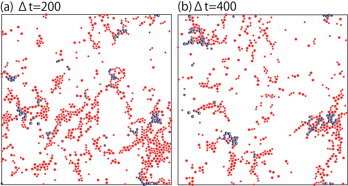
Figure 7: Early-stage snapshots of particles with β„±i=0subscriptℱ𝑖0{\cal F}_{i}=0 at t=200𝑑200t=200 (left) and 400 (right), which are classified into those with ℬi=0subscriptℬ𝑖0{\cal B}_{i}=0 (red) and those with ℬi=1subscriptℬ𝑖1{\cal B}_{i}=1 (blue). Here T=0.56𝑇0.56T=0.56 and N=4000𝑁4000N=4000. Numbers of the former (red) and the latter (blue) are (766,75)76675(766,75) in (a) and (535,81)53581(535,81) in (b). The former arise from the collective vibrational modes emerging for t≳10greater-than-or-equivalent-to𝑑10t\gtrsim 10.

We first examine the fluctuations of the particle positions due to the thermally excited low-frequency vibration modes at low T𝑇T before the onset of the structural relaxation. They exhibit significant heterogeneity, as found by Muranaka and Hiwatari in a very short time interval of width 5 in a 2D soft-core system with N=104𝑁superscript104N=10^{4} Hi .

For tβ‰ͺΟ„b​pmuch-less-than𝑑subscriptπœπ‘π‘t\ll\tau_{bp}, we may neglect the configuration changes from the discussion below Eq.(3.16) and define the dispalcement vector 𝒖i​(t)=𝒓i​(t)βˆ’π’“Β―isubscript𝒖𝑖𝑑subscript𝒓𝑖𝑑subscript¯𝒓𝑖{\mbox{\boldmath$u$}}_{i}(t)={\mbox{\boldmath$r$}}_{i}(t)-{\bar{\mbox{\boldmath$r$}}}_{i}, where 𝒓¯isubscript¯𝒓𝑖{\bar{\mbox{\boldmath$r$}}}_{i} is the time-averaged position in a time interval with width much shorter than Ο„b​psubscriptπœπ‘π‘\tau_{bp}. The equal-time variance ⟨|𝒖|2⟩=βˆ‘i⟨|𝒖i|2⟩/Ndelimited-⟨⟩superscript𝒖2subscript𝑖delimited-⟨⟩superscriptsubscript𝒖𝑖2𝑁\langle{|{\mbox{\boldmath$u$}}|^{2}}\rangle=\sum_{i}\langle{|{\mbox{\boldmath$u$}}_{i}|^{2}}\rangle/N is a half of the plateau value Mpsubscript𝑀pM_{\rm p} of the mean square displacement at low T𝑇T (see Eq.(A5) below). From the appendix, ⟨|𝒖|2⟩delimited-⟨⟩superscript𝒖2\langle{|{\mbox{\boldmath$u$}}|^{2}}\rangle increases with increasing the system length L𝐿L logarithmically in 2D as Janco

⟨|𝒖|2⟩=Mp/2β‰…C0+C1​ln⁑(L/Οƒ1),delimited-⟨⟩superscript𝒖2subscript𝑀p2subscript𝐢0subscript𝐢1𝐿subscript𝜎1\langle{|{\mbox{\boldmath$u$}}|^{2}}\rangle=M_{\rm p}/2\cong C_{0}+C_{1}\ln(L/\sigma_{1}), (4.6)

where C0subscript𝐢0C_{0} and C1subscript𝐢1C_{1} are functions of T𝑇T and are independent of L𝐿L. In terms of the shear modulus ΞΌπœ‡\mu and and the bulk modulus K𝐾K, the coefficient C1subscript𝐢1C_{1} is expressed as

C1=kB​T2​π​(1ΞΌ+1K+ΞΌ).subscript𝐢1subscriptπ‘˜π΅π‘‡2πœ‹1πœ‡1πΎπœ‡C_{1}=\frac{k_{B}T}{2\pi}\bigg{(}\frac{1}{\mu}+\frac{1}{K+\mu}\bigg{)}. (4.7)

In our 2D system, we obtained ΞΌβ‰…18πœ‡18\mu\cong 18 and Kβ‰…67.5𝐾67.5K\cong 67.5 at T=0.56𝑇0.56T=0.56 from the inital linear growth of stress-strain relation and the density-pressure relation (not shown in this paper) sound . Then we find C1β‰…0.0060subscript𝐢10.0060C_{1}\cong 0.0060 at T=0.56𝑇0.56T=0.56. If the total particle number is increased from 400040004000 to 640006400064000, Eq.(4.6) yields the incremental increase C1​ln⁑4β‰…0.0083subscript𝐢140.0083C_{1}\ln 4\cong 0.0083 in ⟨|𝒖|2⟩delimited-⟨⟩superscript𝒖2\langle{|{\mbox{\boldmath$u$}}|^{2}}\rangle. In fair agreement with this estimate, we numerically calculated ⟨|𝒖|2⟩delimited-⟨⟩superscript𝒖2\langle{|{\mbox{\boldmath$u$}}|^{2}}\rangle to be 0.02266 for N=4000𝑁4000N=4000 and 0.03305 for N=64000𝑁64000N=64000, where 𝒓¯isubscript¯𝒓𝑖{\bar{\mbox{\boldmath$r$}}}_{i} was equated with the time-average of 𝒓i​(t)subscript𝒓𝑖𝑑{\mbox{\boldmath$r$}}_{i}(t) in a time interval of width 200.

With Eq.(4.6), we need to examine how the particles remain within or go outside their initial circle. In Fig.5, we display Δ​ri​(t0,t1)Ξ”subscriptπ‘Ÿπ‘–subscript𝑑0subscript𝑑1\Delta r_{i}(t_{0},t_{1}) in Eq.(4.5) for five particles in time range t=t1βˆ’t0<18000𝑑subscript𝑑1subscript𝑑018000t=t_{1}-t_{0}<18000 with N=4000𝑁4000N=4000. These particles are separated from one another with distances longer than 10. We recognize that these displacements undergo rapid thermal fluctuations with magnitudes nearly equal to the overlap length 0.30.30.3. In the early stage (t<Ο„b​p𝑑subscriptπœπ‘π‘t<\tau_{bp}), most of β„±isubscriptℱ𝑖{\cal{F}}_{i} fluctuate between 1 and 0. In this example, two of them escape from their initial circle, where one has a broken bond at t∼8000similar-to𝑑8000t\sim 8000 and the other has two broken bonds at t∼10000similar-to𝑑10000t\sim 10000 (see Fig.6). Each jump itself occurs on a short time of order 10. In (a) of Fig.6 gives the trajectory of the particle escaping from a cage at t∼104similar-to𝑑superscript104t\sim 10^{4} in Fig.5. In (b) of Fig.6, this escape take place as a string-like motion involving several particles as in 3D Kob ; Sc . See (a) of Fig.13 below for other examples. In (b) of Fig.6, we can see that most of the particles involved have only one broken bond, which is particularly the case for isolated configuration changes. Therefore, these motions may also be treated as small slips in 2D.

Removing the rapid temporal fluctuations, we calculated the smoothed displacement lengths,

Δ​rΒ―i​(t)=|𝒓¯i​(t+t0)βˆ’π’“Β―i​(t0)|,Ξ”subscriptΒ―π‘Ÿπ‘–π‘‘subscript¯𝒓𝑖𝑑subscript𝑑0subscript¯𝒓𝑖subscript𝑑0\Delta{\bar{r}}_{i}(t)=|{\bar{\mbox{\boldmath$r$}}}_{i}(t+t_{0})-{\bar{\mbox{\boldmath$r$}}}_{i}(t_{0})|, (4.8)

for the time-smoothed positions,

𝒓¯i​(t)=1tsmβ€‹βˆ«0tsm𝑑t′​𝒓i​(t+tβ€²).subscript¯𝒓𝑖𝑑1subscript𝑑smsuperscriptsubscript0subscript𝑑smdifferential-dsuperscript𝑑′subscript𝒓𝑖𝑑superscript𝑑′{\bar{\mbox{\boldmath$r$}}}_{i}(t)=\frac{1}{t_{\rm sm}}\int_{0}^{t_{\rm sm}}dt^{\prime}{{\mbox{\boldmath$r$}}}_{i}(t+t^{\prime}). (4.9)

In the inset of Fig.5, the smoothing time tsmsubscript𝑑smt_{\rm sm} is 500. Even on this timescale, the particles move considerably, even across their initial circle. Note that this tsmsubscript𝑑smt_{\rm sm} is much longer than the traversal time of the transverse sounds across the system ta=L/cβŸ‚βˆΌ17subscriptπ‘‘π‘ŽπΏsubscript𝑐perpendicular-tosimilar-to17t_{a}=L/c_{\perp}\sim 17 for N=4000𝑁4000N=4000 sound . These complex fluctuations should originate from superposition of weakly coupled, low-frequency vibration modes La ; Angela ; Ganter ; Shintani ; Reichman ; Ruocco ; Barrat ; Liu ; Bonn ; Br ; Sc .
Refer to caption
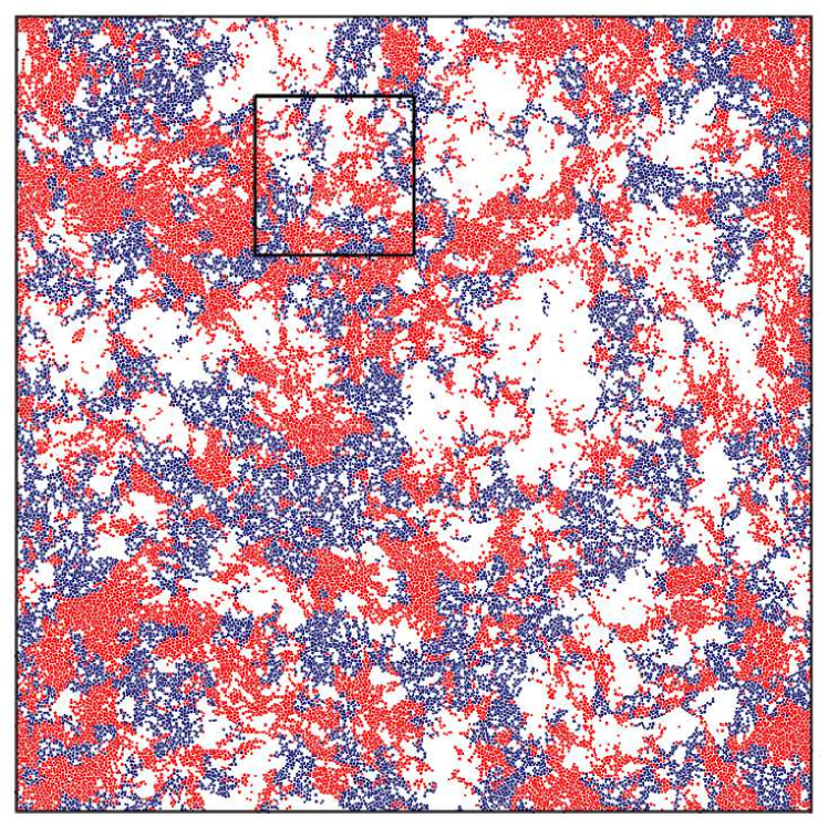
Figure 8: Late-stage snapshot of particles with β„±i=0subscriptℱ𝑖0{\cal F}_{i}=0 in a large system of N=64000𝑁64000N=64000 and L=281𝐿281L=281, where t=104𝑑superscript104t=10^{4} and T=0.56𝑇0.56T=0.56. Depicted particles are classified into those with ℬi=0subscriptℬ𝑖0{\cal B}_{i}=0 (red) and those with ℬiβ‰₯1subscriptℬ𝑖1{\cal B}_{i}\geq 1 (blue). Numbers of the former (red) and the latter (blue) are (22034,18122)2203418122(22034,18122), respectively. The former arise from the low-frequency vibration modes. Subsequent time-evolution in the upper box region will be given in the right of Fig.14.

In Fig.7, we show the particles with β„±i=0subscriptℱ𝑖0{\cal F}_{i}=0 at very early times t=200𝑑200t=200 and 400 for T=0.56𝑇0.56T=0.56 and N=4000𝑁4000N=4000, where their initial circles contain no particle. The fraction of the particles with β„±i=0subscriptℱ𝑖0{\cal F}_{i}=0, written as Ο•4​(t)subscriptitalic-Ο•4𝑑\phi_{4}(t), is soon about 0.2 for t≳10greater-than-or-equivalent-to𝑑10t\gtrsim 10. That is, a considerable amount of the non-𝑩𝑩B particles with β„±i=0subscriptℱ𝑖0{\cal F}_{i}=0 already appear from very early times. However, some of the 𝑩𝑩B particles depicted at t=200𝑑200t=200 are changed to those with β„±i=1subscriptℱ𝑖1{\cal F}_{i}=1 at t=400𝑑400t=400 (see the sentences at the end of Sec.IVA).

In Fig.8, we show the particles with β„±i=0subscriptℱ𝑖0{\cal F}_{i}=0 at t=104βˆΌΟ„Ξ±π‘‘superscript104similar-tosubscriptπœπ›Όt=10^{4}\sim\tau_{\alpha} for T=0.56𝑇0.56T=0.56 in a much larger system of N=64000𝑁64000N=64000. Some heterogeneities have sizes of order 50. Among the displayed particles, the 𝑩𝑩B and non-𝑩𝑩B particles amount to 22034 and 18122, respectively. The patterns of the latter are more extended than those of the former. Moreover, their timescales are distinctly separated (see Fig.14 below). These indicate the presence of thermally excited large-scale vibration modes.

IV.3 Four-point correlations
Refer to caption
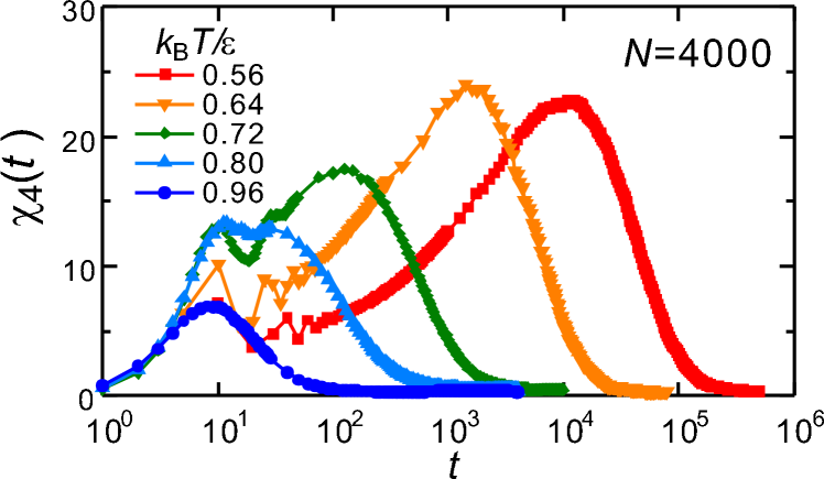
Figure 9: Susceptibility Ο‡4​(t)subscriptπœ’4𝑑\chi_{4}(t) in Eq.(4.14) vs t𝑑t for N=4000𝑁4000N=4000.
Refer to caption
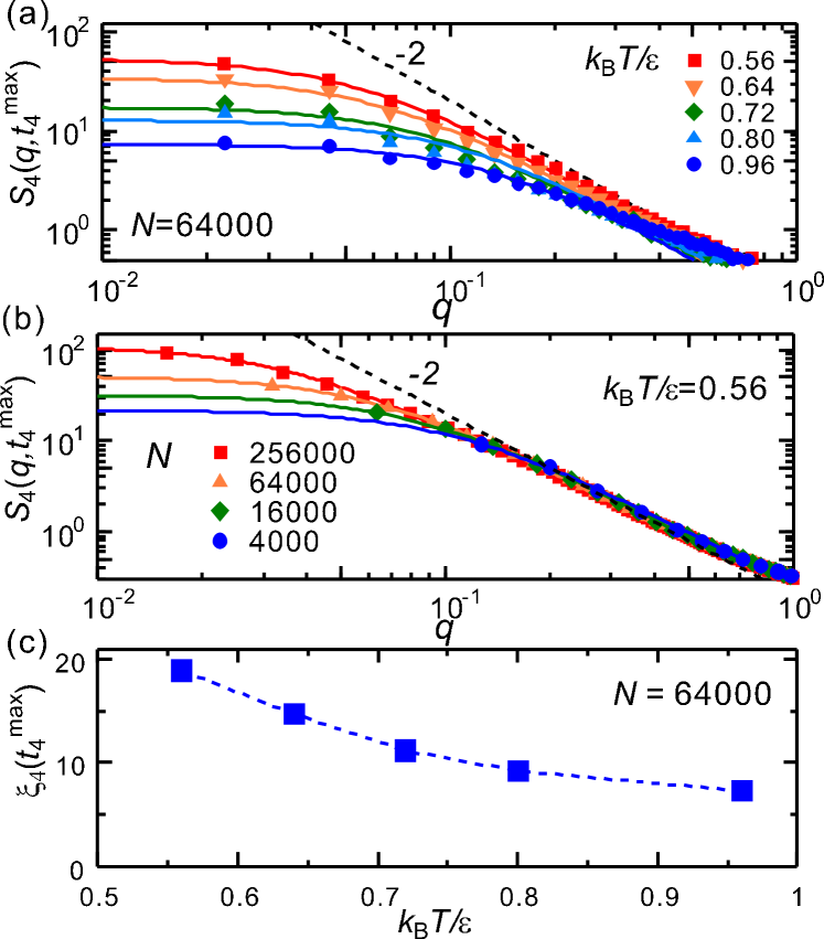
Figure 10: (a) Four-point structure factor S4​(q,t4max)subscript𝑆4π‘žsuperscriptsubscript𝑑4maxS_{4}(q,t_{4}^{\rm max}) vs qπ‘žq in Eq.(4.13) for various T𝑇T, where N=64000𝑁64000N=64000. (b) S4​(q,t4max)subscript𝑆4π‘žsuperscriptsubscript𝑑4maxS_{4}(q,t_{4}^{\rm max}) vs qπ‘žq for various N𝑁N at T=0.56𝑇0.56T=0.56. (c) ΞΎ4​(t4max)subscriptπœ‰4superscriptsubscript𝑑4max\xi_{4}(t_{4}^{\rm max}) for N=64000𝑁64000N=64000. Marked system-size dependence appears at small qπ‘žq due to the low-frequency vibration modes.

The average of 𝒬^​(𝒓,t0,t1)^𝒬𝒓subscript𝑑0subscript𝑑1\hat{\cal{Q}}({\mbox{\boldmath$r$}},t_{0},t_{1}) in Eq.(4.1) is written as

q4​(t)subscriptπ‘ž4𝑑\displaystyle q_{4}(t) =\displaystyle= βŸ¨π’¬^​(𝒓,t0,t1)⟩delimited-⟨⟩^𝒬𝒓subscript𝑑0subscript𝑑1\displaystyle\langle{\hat{\cal{Q}}({\mbox{\boldmath$r$}},t_{0},t_{1})}\rangle (4.10)
=\displaystyle= 1Vβ€‹βˆ‘i​jw​(|𝒓i​(t0)βˆ’π’“j​(t1)|),1𝑉subscript𝑖𝑗𝑀subscript𝒓𝑖subscript𝑑0subscript𝒓𝑗subscript𝑑1\displaystyle\frac{1}{V}\sum_{ij}w(|{\mbox{\boldmath$r$}}_{i}(t_{0})-{\mbox{\boldmath$r$}}_{j}(t_{1})|),

which is a function of t=t1βˆ’t0𝑑subscript𝑑1subscript𝑑0t=t_{1}-t_{0}. In our simulation, β„±i=1subscriptℱ𝑖1{\cal F}_{i}=1 or 0, so q4​(t)subscriptπ‘ž4𝑑q_{4}(t) is related to the fraction Ο•4​(t)subscriptitalic-Ο•4𝑑\phi_{4}(t) of the particles with β„±i=0subscriptℱ𝑖0{\cal F}_{i}=0 as

q4​(t)=n​[1βˆ’Ο•4​(t)].subscriptπ‘ž4𝑑𝑛delimited-[]1subscriptitalic-Ο•4𝑑q_{4}(t)=n[1-\phi_{4}(t)]. (4.11)

Here, q4​(0)=nsubscriptπ‘ž40𝑛q_{4}(0)=n and q4​(∞)=v0​n2subscriptπ‘ž4subscript𝑣0superscript𝑛2q_{4}(\infty)=v_{0}n^{2}, where v0subscript𝑣0v_{0} is the area or volume of the overlap region (v0=π​(A4​σ1)2subscript𝑣0πœ‹superscriptsubscript𝐴4subscript𝜎12v_{0}=\pi(A_{4}\sigma_{1})^{2} in 2D and v0=4​π​(A4​σ1)3/3subscript𝑣04πœ‹superscriptsubscript𝐴4subscript𝜎133v_{0}=4\pi(A_{4}\sigma_{1})^{3}/3 in 3D).

As in Eq.(3.19) for Gb​(r,t)subscriptπΊπ‘π‘Ÿπ‘‘G_{b}({r},t), the four-point space-time correlation function is given by

G4​(r,t)subscript𝐺4π‘Ÿπ‘‘\displaystyle G_{4}({r},t) =\displaystyle= βŸ¨π’¬^​(𝒓+𝒓′,t0,t1)​𝒬^​(𝒓′,t0,t1)⟩delimited-⟨⟩^𝒬𝒓superscript𝒓′subscript𝑑0subscript𝑑1^𝒬superscript𝒓′subscript𝑑0subscript𝑑1\displaystyle\langle{\hat{\cal{Q}}({\mbox{\boldmath$r$}}+{\mbox{\boldmath$r$}}^{\prime},t_{0},t_{1})\hat{\cal{Q}}({\mbox{\boldmath$r$}}^{\prime},t_{0},t_{1})}\rangle (4.12)
=1Vβ€‹βŸ¨βˆ‘i​kβ„±i​(t0,t1)​ℱk​(t0,t1)​δ​(π’“βˆ’π’“i​k​(t0))⟩,absent1𝑉delimited-⟨⟩subscriptπ‘–π‘˜subscriptℱ𝑖subscript𝑑0subscript𝑑1subscriptβ„±π‘˜subscript𝑑0subscript𝑑1𝛿𝒓subscriptπ’“π‘–π‘˜subscript𝑑0\displaystyle=\frac{1}{V}{\bigg{\langle}}{\sum_{ik}{\cal F}_{i}(t_{0},t_{1}){\cal F}_{k}(t_{0},t_{1})\delta({\mbox{\boldmath$r$}}-{\mbox{\boldmath$r$}}_{ik}(t_{0}))}{\bigg{\rangle}},

where 𝒓i​k​(t0)=𝒓i​(t0)βˆ’π’“k​(t0)subscriptπ’“π‘–π‘˜subscript𝑑0subscript𝒓𝑖subscript𝑑0subscriptπ’“π‘˜subscript𝑑0{\mbox{\boldmath$r$}}_{ik}(t_{0})={\mbox{\boldmath$r$}}_{i}(t_{0})-{\mbox{\boldmath$r$}}_{k}(t_{0}). The four-point structure factor is defined by

S4​(q,t)subscript𝑆4π‘žπ‘‘\displaystyle S_{4}(q,t) =\displaystyle= 1Vβ€‹βŸ¨|𝒬^𝒒​(t0,t1)|2⟩1𝑉delimited-⟨⟩superscriptsubscript^𝒬𝒒subscript𝑑0subscript𝑑12\displaystyle\frac{1}{V}\langle{|{\hat{\cal Q}}_{\mbox{\boldmath$q$}}(t_{0},t_{1})|^{2}}\rangle (4.13)
=βˆ«π‘‘π’“β€‹[G4​(r,t)βˆ’q4​(t)2]​ei​𝒒⋅𝒓,absentdifferential-d𝒓delimited-[]subscript𝐺4π‘Ÿπ‘‘subscriptπ‘ž4superscript𝑑2superscript𝑒⋅𝑖𝒒𝒓\displaystyle=\int d{\mbox{\boldmath$r$}}[G_{4}({r},t)-q_{4}(t)^{2}]e^{i{\mbox{\boldmath$q$}}\cdot{\mbox{\boldmath$r$}}},

where 𝒬^𝒒​(t0,t1)=βˆ‘jβ„±j​(t0,t1)​exp⁑[i​𝒒⋅𝒓j​(t0)]subscript^𝒬𝒒subscript𝑑0subscript𝑑1subscript𝑗subscriptℱ𝑗subscript𝑑0subscript𝑑1⋅𝑖𝒒subscript𝒓𝑗subscript𝑑0{\hat{\cal Q}}_{\mbox{\boldmath$q$}}(t_{0},t_{1})=\sum_{j}{\cal F}_{j}(t_{0},t_{1})\exp[i{\mbox{\boldmath$q$}}\cdot{\mbox{\boldmath$r$}}_{j}(t_{0})] is the Fourier component of 𝒬^​(𝒓,t0,t1)^𝒬𝒓subscript𝑑0subscript𝑑1{\hat{\cal Q}}({\mbox{\boldmath$r$}},t_{0},t_{1}). We define the four-point susceptibility Ο‡4​(t)subscriptπœ’4𝑑\chi_{4}(t) by

Ο‡4​(t)=1Vβ€‹βŸ¨βˆ‘i​kδ​ℱi​(t0,t1)​δ​ℱk​(t0,t1)⟩.subscriptπœ’4𝑑1𝑉delimited-⟨⟩subscriptπ‘–π‘˜π›Ώsubscriptℱ𝑖subscript𝑑0subscript𝑑1𝛿subscriptβ„±π‘˜subscript𝑑0subscript𝑑1\chi_{4}(t)=\frac{1}{V}{\bigg{\langle}}{\sum_{ik}\delta{\cal F}_{i}(t_{0},t_{1})\delta{\cal F}_{k}(t_{0},t_{1})}{\bigg{\rangle}}. (4.14)

in terms of the deviation δ​ℱi​(t0,t1)=β„±i​(t0,t1)βˆ’q4​(t)/n𝛿subscriptℱ𝑖subscript𝑑0subscript𝑑1subscriptℱ𝑖subscript𝑑0subscript𝑑1subscriptπ‘ž4𝑑𝑛\delta{\cal F}_{i}(t_{0},t_{1})={\cal F}_{i}(t_{0},t_{1})-q_{4}(t)/n. In these correlation functions, the four particle positions 𝒓i​(t0)subscript𝒓𝑖subscript𝑑0{\mbox{\boldmath$r$}}_{i}(t_{0}), 𝒓k​(t0)subscriptπ’“π‘˜subscript𝑑0{\mbox{\boldmath$r$}}_{k}(t_{0}), 𝒓j​(t1)subscript𝒓𝑗subscript𝑑1{\mbox{\boldmath$r$}}_{j}(t_{1}), and 𝒓ℓ​(t1)subscript𝒓ℓsubscript𝑑1{\mbox{\boldmath$r$}}_{\ell}(t_{1}) are involved. However, as discussed around Eq.(4.4), the self parts with i=j𝑖𝑗i=j and k=β„“π‘˜β„“k=\ell dominate over the distinct parts with iβ‰ j𝑖𝑗i\neq j and kβ‰ β„“π‘˜β„“k\neq\ell Lacevic .

Berthier et al.b1 ; b2 showed that the four-point susceptibility Ο‡4​(t)subscriptπœ’4𝑑\chi_{4}(t) depends on the ensemble (N​V​E𝑁𝑉𝐸NVE or N​V​T𝑁𝑉𝑇NVT) and the dynamics (Newtonian or Brownian). Our Ο‡4​(t4max)subscriptπœ’4superscriptsubscript𝑑4max\chi_{4}(t_{4}^{\rm max}) in the N​V​E𝑁𝑉𝐸NVE ensemble is roughly 60%percent6060\% of the long wavelength limit of the four-point structure factor Ο‡40​(t4max)=limqβ†’0S4​(q,t4max)subscriptsuperscriptπœ’04superscriptsubscript𝑑4maxsubscriptβ†’π‘ž0subscript𝑆4π‘žsuperscriptsubscript𝑑4max\chi^{0}_{4}(t_{4}^{\rm max})=\lim_{q\to 0}S_{4}(q,t_{4}^{\rm max}), which is consistent with the previous calculations b1 ; b2 ; Chandler ; Szamel ; Sas . However, in our calculation, the long wavelength limit of the bond-breakage structure factor Ο‡b0​(tbmax)=limqβ†’0Sb​(q,tbmax)subscriptsuperscriptπœ’0𝑏superscriptsubscript𝑑𝑏maxsubscriptβ†’π‘ž0subscriptπ‘†π‘π‘žsuperscriptsubscript𝑑𝑏max\chi^{0}_{b}(t_{b}^{\rm max})=\lim_{q\to 0}S_{b}(q,t_{b}^{\rm max}) cannot be determined reliably because of the very long tbmaxsuperscriptsubscript𝑑𝑏maxt_{b}^{\rm max} at low T𝑇T (see Fig.4) and our maximum bond-breakage susceptibility Ο‡b​(tbmax)subscriptπœ’π‘superscriptsubscript𝑑𝑏max\chi_{b}(t_{b}^{\rm max}) in Fig.3 apparently exceeds Ο‡b0​(tbmax)subscriptsuperscriptπœ’0𝑏superscriptsubscript𝑑𝑏max\chi^{0}_{b}(t_{b}^{\rm max}) by a few ten %percent\%. Thus, we cannot draw a definite conclusion on the relation between Ο‡b​(tbmax)subscriptπœ’π‘superscriptsubscript𝑑𝑏max\chi_{b}(t_{b}^{\rm max}) and Ο‡b0​(tbmax)subscriptsuperscriptπœ’0𝑏superscriptsubscript𝑑𝑏max\chi^{0}_{b}(t_{b}^{\rm max}).

In (a) of Fig.9, we give Ο‡4​(t)subscriptπœ’4𝑑\chi_{4}(t) in Eq.(4.14) as a function of t𝑑t for various T𝑇T, which is calculated in the N​V​E𝑁𝑉𝐸NVE ensemble with N=4000𝑁4000N=4000. It is maximized at t=t4max𝑑superscriptsubscript𝑑4maxt=t_{4}^{\rm max}. Here, due to the transverse sound propagation, a smaller acoustic peak emerges with lowering T𝑇T at t=ta/2∼8.6𝑑subscriptπ‘‘π‘Ž2similar-to8.6t=t_{a}/2\sim 8.6 sound , whose existence has not been reported in the previous papers. It becomes more evident at lower T𝑇T, where the acoustic damping is weaker. We also calculated Ο‡4​(t)subscriptπœ’4𝑑\chi_{4}(t) for other N𝑁N. For N=64000𝑁64000N=64000, the acoustic peak was at t∼34similar-to𝑑34t\sim 34 and its height even exceeded the first peak height for low T𝑇T. For N=1000𝑁1000N=1000, there was no acoustic peak. See the item (3) in the summary for more discussions.

La ̌ceviΔ‡ et al.Lacevic determined the overlap length a​σ2π‘Žsubscript𝜎2a\sigma_{2} to maximize the peak height of the four-point susceptibility Ο‡4​(t4max)subscriptπœ’4superscriptsubscript𝑑4max\chi_{4}(t_{4}^{\rm max}) as a function of the parameter aπ‘Ža at T=0.59𝑇0.59T=0.59 in 3D. They then obtained a=0.3π‘Ž0.3a=0.3 and used it also at other low T𝑇T. Following their method, we also maximized Ο‡4​(t4max)subscriptπœ’4superscriptsubscript𝑑4max\chi_{4}(t_{4}^{\rm max}) as a function of the overlap length to obtain A4=0.3subscript𝐴40.3A_{4}=0.3 in Eq.(4.3) for T=0.64𝑇0.64T=0.64 and N=4000𝑁4000N=4000. Then t4max∼104similar-tosuperscriptsubscript𝑑4maxsuperscript104t_{4}^{\rm max}\sim 10^{4} at T=0.56𝑇0.56T=0.56 both for N=4000𝑁4000N=4000 and 64000.

In (a) of Fig.10, we plot S4​(q,t4max)subscript𝑆4π‘žsuperscriptsubscript𝑑4maxS_{4}(q,t_{4}^{\rm max}) vs qπ‘žq for various T𝑇T with N=64000𝑁64000N=64000. In its calculation, we took the average over the initial time t0subscript𝑑0t_{0} in the wide range [0,106]0superscript106[0,10^{6}]. As in the case of Sb​(q,t)subscriptπ‘†π‘π‘žπ‘‘S_{b}(q,t) in Eq.(3.20), we may fit S4​(q,t)subscript𝑆4π‘žπ‘‘S_{4}(q,t) to the Ornstein-Zernike form as Lacevic

S4​(q,t)=Ο‡40​(t)/[1+q2​ξ4​(t)2],subscript𝑆4π‘žπ‘‘superscriptsubscriptπœ’40𝑑delimited-[]1superscriptπ‘ž2subscriptπœ‰4superscript𝑑2S_{4}(q,t)=\chi_{4}^{0}(t)/[1+q^{2}\xi_{4}(t)^{2}], (4.15)

where Ο‡40​(t)=limqβ†’0S4​(q,t)superscriptsubscriptπœ’40𝑑subscriptβ†’π‘ž0subscript𝑆4π‘žπ‘‘\chi_{4}^{0}(t)=\lim_{q\to 0}S_{4}(q,t) is the long wavelength limit of S4​(q,t)subscript𝑆4π‘žπ‘‘S_{4}(q,t) and ΞΎ4​(t)subscriptπœ‰4𝑑\xi_{4}(t) is the four-point correlation length. Furthermore, in (b), we show S4​(q,t4max)subscript𝑆4π‘žsuperscriptsubscript𝑑4maxS_{4}(q,t_{4}^{\rm max}) at T=0.56𝑇0.56T=0.56 for various N𝑁N up to N=256000𝑁256000N=256000 to demonstrate its significant system-size dependence at small qπ‘žq. In (c), we display ΞΎ4​(t4max)subscriptπœ‰4superscriptsubscript𝑑4max\xi_{4}(t_{4}^{\rm max}) vs T𝑇T for N=64000𝑁64000N=64000 as an example, which increases with lowering T𝑇T. We recognize that the ratio ΞΎ4​(t4max)/ΞΎb​(tbmax)subscriptπœ‰4superscriptsubscript𝑑4maxsubscriptπœ‰π‘superscriptsubscript𝑑𝑏max\xi_{4}(t_{4}^{\rm max})/\xi_{b}(t_{b}^{\rm max}) exceeds unity and increases with increasing N𝑁N. For example, it is about 3 for T=0.56𝑇0.56T=0.56 and N=64000𝑁64000N=64000. Thus, on our 2D simulation, the effect of the low-frequency vibration modes on the four-point correlations becomes stronger for larger N𝑁N.

Refer to caption
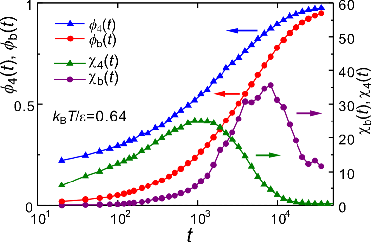
Figure 11: Fraction Ο•b​(t)subscriptitalic-ϕ𝑏𝑑\phi_{b}(t) and susceptibility Ο‡b​(t)subscriptπœ’π‘π‘‘\chi_{b}(t) for bond breakage and those Ο•4​(t)subscriptitalic-Ο•4𝑑\phi_{4}(t) and Ο‡4​(t)subscriptπœ’4𝑑\chi_{4}(t) for four-point correlations for T=0.64𝑇0.64T=0.64 and N=4000𝑁4000N=4000. Here, Ο‡b​(t)subscriptπœ’π‘π‘‘\chi_{b}(t) and Ο‡4​(t)subscriptπœ’4𝑑\chi_{4}(t) are maximized for Ο•b​(t)∼1/2similar-tosubscriptitalic-ϕ𝑏𝑑12\phi_{b}(t)\sim 1/2 and Ο•4​(t)∼1/2similar-tosubscriptitalic-Ο•4𝑑12\phi_{4}(t)\sim 1/2, respectively.
Refer to caption
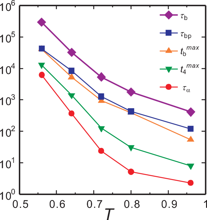
Figure 12: Relaxation times as functions of T𝑇T for the soft-core potential for N=4000𝑁4000N=4000 in 2D. From above, they are Ο„bsubscriptπœπ‘\tau_{b} in Eq.(3.4), Ο„b​psubscriptπœπ‘π‘\tau_{bp} in Eq.(3.16), tbmaxsuperscriptsubscript𝑑𝑏maxt_{b}^{\rm max} from the maximum of Ο‡b​(t)subscriptπœ’π‘π‘‘\chi_{b}(t), t4maxsuperscriptsubscript𝑑4maxt_{4}^{\rm max} from the maximum of Ο‡4​(t)subscriptπœ’4𝑑\chi_{4}(t), and ταsubscriptπœπ›Ό\tau_{\alpha} in Eq.(3.6).
Refer to caption
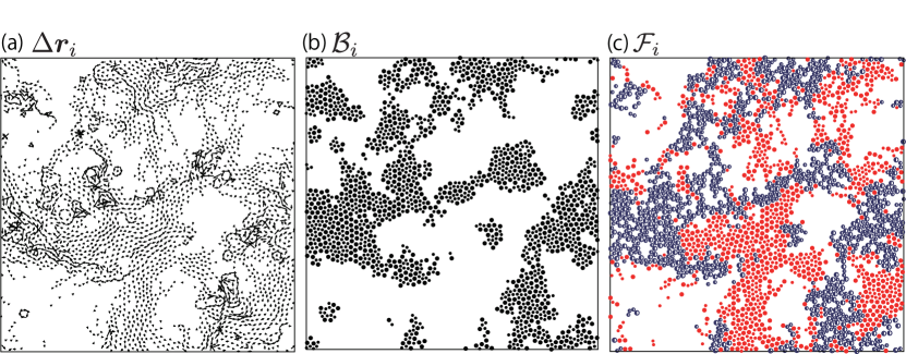
Figure 13: Snapshots at t=t1βˆ’t0=104𝑑subscript𝑑1subscript𝑑0superscript104t=t_{1}-t_{0}=10^{4} for T=0.56𝑇0.56T=0.56 and N=4000𝑁4000N=4000 in 2D. System length is L=70.2𝐿70.2L=70.2. (a) Displacements Δ​𝒓i​(t0,t1)Ξ”subscript𝒓𝑖subscript𝑑0subscript𝑑1\Delta{\mbox{\boldmath$r$}}_{i}(t_{0},t_{1}) with |Δ​𝒓i|>0.3Ξ”subscript𝒓𝑖0.3|\Delta{\mbox{\boldmath$r$}}_{i}|>0.3, (b) 𝑩𝑩B particles, and (c) those with β„±i=0subscriptℱ𝑖0{\cal F}_{i}=0 classified into 𝑩𝑩B particles (blue) and non-𝑩𝑩B particles (red). Non-𝑩𝑩B particles with β„±i=0subscriptℱ𝑖0{\cal F}_{i}=0 are produced by collective motions, while most 𝑩𝑩B particles participate in string-like motions and satisfy β„±i=0subscriptℱ𝑖0{\cal F}_{i}=0.
Refer to caption
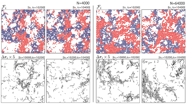
Figure 14: Snapshots at t=10000+200​k𝑑10000200π‘˜t=10000+200k (k=1,2π‘˜12k=1,2) at T=0.56𝑇0.56T=0.56 for N=4000𝑁4000N=4000 (left) and for N=64000𝑁64000N=64000 (right). Top: Particles with β„±i=0subscriptℱ𝑖0{\cal F}_{i}=0 classified into non-𝑩𝑩B particles (red) and 𝑩𝑩B particles (blue), where the former significantly change but the latter little change in this short time interval. The change of the former is larger for the larger N𝑁N in the right. See the preceding snapshots in (c) of Fig.13 for N=4000𝑁4000N=4000 and in the black box of Fig.8 for N=64000𝑁64000N=64000. Bottom: Displacements Δ​𝒓i=Δ​𝒓i​(t0+tβ€²,t0+tβ€²+200)Ξ”subscript𝒓𝑖Δsubscript𝒓𝑖subscript𝑑0superscript𝑑′subscript𝑑0superscript𝑑′200\Delta{\mbox{\boldmath$r$}}_{i}=\Delta{\mbox{\boldmath$r$}}_{i}(t_{0}+t^{\prime},t_{0}+t^{\prime}+200) multiplied by 5 with |Δ​𝒓i|>0.3Ξ”subscript𝒓𝑖0.3|\Delta{\mbox{\boldmath$r$}}_{i}|>0.3 in short time intervals of 200, where tβ€²=10000superscript𝑑′10000t^{\prime}=10000 or 10200.

V Comparison of the two theoretical schemes

V.1 Timescales

In Fig.11, we display Ο•b​(t)subscriptitalic-ϕ𝑏𝑑\phi_{b}(t), Ο•4​(t)subscriptitalic-Ο•4𝑑\phi_{4}(t), Ο‡b​(t)subscriptπœ’π‘π‘‘\chi_{b}(t), and Ο‡4​(t)subscriptπœ’4𝑑\chi_{4}(t) at T=0.64𝑇0.64T=0.64 for N=4000𝑁4000N=4000 in the two theoreticaal schemes. Here, Ο•b​(t)subscriptitalic-ϕ𝑏𝑑\phi_{b}(t) is the fraction of the particles with ℬi>0subscriptℬ𝑖0{\cal B}_{i}>0 and Ο•4​(t)subscriptitalic-Ο•4𝑑\phi_{4}(t) is that with β„±i=0subscriptℱ𝑖0{\cal F}_{i}=0. We can see that Ο•b∼1/2similar-tosubscriptitalic-ϕ𝑏12\phi_{b}\sim 1/2 at t=tbmax𝑑superscriptsubscript𝑑𝑏maxt=t_{b}^{\rm max} and Ο•4∼1/2similar-tosubscriptitalic-Ο•412\phi_{4}\sim 1/2 at t=t4max𝑑superscriptsubscript𝑑4maxt=t_{4}^{\rm max}. If Ο•b​(t)subscriptitalic-ϕ𝑏𝑑\phi_{b}(t) (or Ο•4​(t)subscriptitalic-Ο•4𝑑\phi_{4}(t)) is close to 0 or 1, Sb​(q,t)subscriptπ‘†π‘π‘žπ‘‘S_{b}(q,t) (or Sb​(q,t)subscriptπ‘†π‘π‘žπ‘‘S_{b}(q,t)) becomes very small.

So far we have introduced the bond-breakage time Ο„bsubscriptπœπ‘\tau_{b} in Eq.(3.4), the relaxation time ταsubscriptπœπ›Ό\tau_{\alpha} from Fs​(q,t)subscriptπΉπ‘ π‘žπ‘‘F_{s}(q,t) in Eq.(3.6), the bond-preserving time Ο„b​psubscriptπœπ‘π‘\tau_{bp} in Eq.(3.16), the maximization time tbmaxsuperscriptsubscript𝑑𝑏maxt_{b}^{\rm max} of Ο‡b​(t)subscriptπœ’π‘π‘‘\chi_{b}(t) in (a) of Fig.3, and the maximization time t4maxsuperscriptsubscript𝑑4maxt_{4}^{\rm max} of Ο‡4​(t)subscriptπœ’4𝑑\chi_{4}(t) in Fig.9. In Fig.12, these times are in the following order,

τα<t4max<tbmaxβˆΌΟ„b​p<Ο„b,subscriptπœπ›Όsuperscriptsubscript𝑑4maxsuperscriptsubscript𝑑𝑏maxsimilar-tosubscriptπœπ‘π‘subscriptπœπ‘\tau_{\alpha}<t_{4}^{\rm max}<t_{b}^{\rm max}\sim\tau_{bp}<\tau_{b}, (5.1)

with 35≀τb/τα≀10235subscriptπœπ‘subscriptπœπ›Όsuperscript10235\leq\tau_{b}/\tau_{\alpha}\leq 10^{2} in the range 0.56≀T≀0.960.56𝑇0.960.56\leq T\leq 0.96 for N=4000𝑁4000N=4000. In our 2D simulation, ταsubscriptπœπ›Ό\tau_{\alpha} and t4maxsuperscriptsubscript𝑑4maxt_{4}^{\rm max} exhibit strong system-size dependence due to the low-frequency vibration modes. In fact, we numerically obtained τα=8400subscriptπœπ›Ό8400\tau_{\alpha}=8400 for N=4000𝑁4000N=4000 and τα=2140subscriptπœπ›Ό2140\tau_{\alpha}=2140 for N=64000𝑁64000N=64000 (see the appendix). It is worth noting that significant system-size dependence of the plateau behavior of Fs​(q,t)subscriptπΉπ‘ π‘žπ‘‘F_{s}(q,t) (and ταsubscriptπœπ›Ό\tau_{\alpha} from Eq.(3.6)) has been reported in 2D and 3D simulations finite ; Sas ; Kim . Furthermore, Karmakar et al. Sas examined system size-dependence of ΞΎ4subscriptπœ‰4\xi_{4} and S4​(q,t)subscript𝑆4π‘žπ‘‘S_{4}(q,t) up to N=351232𝑁351232N=351232 in 3D.

In addition, we comment on the stress-time-correlation function, which considerably decreases in the early stage due to the thermal motions as well as Fs​(q,t)subscriptπΉπ‘ π‘žπ‘‘F_{s}(q,t). As a result, its relaxation time is of order ταsubscriptπœπ›Ό\tau_{\alpha} Furukawa , while the nonlinear flow behavior is characterized by Ο„bsubscriptπœπ‘\tau_{b} yo1 .

V.2 Time-evolution on long and short timescales

In (a) of Fig.13, the arrows represent relatively large displacements Δ​𝒓i=𝒓i​(t1)βˆ’π’“i​(t0)Ξ”subscript𝒓𝑖subscript𝒓𝑖subscript𝑑1subscript𝒓𝑖subscript𝑑0\Delta{\mbox{\boldmath$r$}}_{i}={\mbox{\boldmath$r$}}_{i}(t_{1})-{\mbox{\boldmath$r$}}_{i}(t_{0}) with |Δ​𝒓i|>0.3Ξ”subscript𝒓𝑖0.3|\Delta{\mbox{\boldmath$r$}}_{i}|>0.3 Hi ; Dol . We can see both large-amplitude string-like motions and smaller-amplitude collective motions. In (b), all the 𝑩𝑩B particles are displayed. In (c), those with β„±i=0subscriptℱ𝑖0{\cal F}_{i}=0 are divided into 𝑩𝑩B and non-𝑩𝑩B particles, where the former exhibit patterns closely resembling those of the 𝑩𝑩B particles in (b). The number of the 𝑩𝑩B particles with β„±i=0subscriptℱ𝑖0{\cal F}_{i}=0 is about 70%percent7070\% of that of the total 𝑩𝑩B particles in (b).

From (a) and (c) of Fig.13, the non-𝑩𝑩B particles with β„±i=0subscriptℱ𝑖0{\cal F}_{i}=0 mostly arise from the collective motions on large scales, as has been the case at short times in Fig.7. Their selection is very sensitive to the overlap length, a​σ2π‘Žsubscript𝜎2a\sigma_{2} in the original workLacevic and A4​σ1subscript𝐴4subscript𝜎1A_{4}\sigma_{1} in this paper, while the 𝑩𝑩B particles (even with β„±i=0subscriptℱ𝑖0{\cal F}_{i}=0) are relatively insensitive to it. In the four-point theory Lacevic , the overlap length was chosen to maximize Ο‡4max=Ο‡4​(t4max)superscriptsubscriptπœ’4maxsubscriptπœ’4superscriptsubscript𝑑4max\chi_{4}^{\rm max}=\chi_{4}(t_{4}^{\rm max}), as discussed above Eq.(4.15). Roughly speaking, their method is to maximize the contribution from the thermal collective motions of non-𝑩𝑩B particles to Ο‡4​(t)subscriptπœ’4𝑑\chi_{4}(t) (see Fig.11).

Table 1: Particle numbers with (a) ℬi>0subscriptℬ𝑖0{\cal B}_{i}>0, (b) ℬi>0subscriptℬ𝑖0{\cal B}_{i}>0 and β„±i=0subscriptℱ𝑖0{\cal F}_{i}=0, (c) ℬi=β„±i=0subscriptℬ𝑖subscriptℱ𝑖0{\cal B}_{i}={\cal F}_{i}=0, and (d) Δ​ri>0.3Ξ”subscriptπ‘Ÿπ‘–0.3\Delta r_{i}>0.3 in Fig.14 at t=10200𝑑10200t=10200 and 10400 for N=4000𝑁4000N=4000 and 64000 in 2D. Those of the particles common in these two shots are also given. Subscript i𝑖i is omitted from Δ​riΞ”subscriptπ‘Ÿπ‘–\Delta r_{i}, ℬisubscriptℬ𝑖{\cal B}_{i}, and β„±isubscriptℱ𝑖{\cal F}_{i}.
t𝑑t (N𝑁N) ℬ>0ℬ0{\cal B}>0~{}~{} ℬ>0ℬ0{\cal B}>0,β„±=0β„±0{\cal F}=0 ℬ=β„±=0ℬℱ0{\cal B}={\cal F}=0 Δ​r>0.3Ξ”π‘Ÿ0.3\Delta r>0.3
102001020010200(4000) 1629 1104 1091 2451
104001040010400(4000) 1667 1180 1221 2643
common(4000) 1576 925 823 1923
102001020010200(64000) 26188 18336 20884 43544
104001040010400(64000) 26413 18678 21785 44693
common(64000) 25192 14149 14349 31790
Table 2: Numbers of non-𝑩𝑩B and 𝑩𝑩B particles for three categories in Fig.14 at t=10200𝑑10200t=10200 for N=4000𝑁4000N=4000 in 2D.
Δ​r>0.3Ξ”π‘Ÿ0.3{\Delta r}>0.3 Δ​r>0.3Ξ”π‘Ÿ0.3{\Delta r}>0.3 Δ​r<0.3Ξ”π‘Ÿ0.3{\Delta r}<0.3
β„±=0β„±0{\cal F}=0 β„±=1β„±1{\cal F}=1 β„±=1β„±1{\cal F}=1 total
ℬ=0ℬ0{\cal B}=0 1091 7 1273 2371
ℬ>0ℬ0{\cal B}>0 1104 249 276 1629
total 2195 256 1549 4000

We next examine time-evolution at two consecutive times t=10200𝑑10200t=10200 and 10400 for N=4000𝑁4000N=4000 (left) and 64000 (right) at T=0.56𝑇0.56T=0.56. The four upper panels of Fig.14 display the particles with β„±i​(t0,t0+t)=0subscriptℱ𝑖subscript𝑑0subscript𝑑0𝑑0{\cal F}_{i}(t_{0},t_{0}+t)=0 grouped into 𝑩𝑩B and non-𝑩𝑩B particles. These snapshots are subsequent to that in (c) of Fig.13 for N=4000𝑁4000N=4000 and that in the box region in Fig.8 for N=64000𝑁64000N=64000 in the same runs. The four lower panels of Fig.14 give the corresponding displacements Δ​𝒓i​(t0+tβ€²,t0+tβ€²+200)Ξ”subscript𝒓𝑖subscript𝑑0superscript𝑑′subscript𝑑0superscript𝑑′200\Delta{\mbox{\boldmath$r$}}_{i}(t_{0}+t^{\prime},t_{0}+t^{\prime}+200) with tβ€²=10000superscript𝑑′10000t^{\prime}=10000 or 10200, which exceed 0.3 in this short time intervals of 200. The differences between the consecutive patterns are evidently larger for N=64000𝑁64000N=64000 than for N=4000𝑁4000N=4000. We can see that this system-size dependence originates from the large-scale vibrational motions.

In Table I, we give the numbers of the particles with (a) ℬi>0subscriptℬ𝑖0{\cal B}_{i}>0, (b) ℬi>0subscriptℬ𝑖0{\cal B}_{i}>0 and β„±i=0subscriptℱ𝑖0{\cal F}_{i}=0, (c) ℬi=β„±i=0subscriptℬ𝑖subscriptℱ𝑖0{\cal B}_{i}={\cal F}_{i}=0, and (d) Δ​ri>0.3Ξ”subscriptπ‘Ÿπ‘–0.3\Delta r_{i}>0.3 in the four snapshots in Fig.14. We also give those of the particles commonly depicted in the consecutive snapshots. In Table II, the numbers of the 𝑩𝑩B and non-𝑩𝑩B particles are given at t=10200𝑑10200t=10200 for (a) Δ​ri>0.3Ξ”subscriptπ‘Ÿπ‘–0.3{\Delta r}_{i}>0.3 and β„±i=0subscriptℱ𝑖0{\cal F}_{i}=0, (b) Δ​ri>0.3Ξ”subscriptπ‘Ÿπ‘–0.3{\Delta r}_{i}>0.3 and β„±i=1subscriptℱ𝑖1{\cal F}_{i}=1, and (c) Δ​ri<0.3Ξ”subscriptπ‘Ÿπ‘–0.3{\Delta r}_{i}<0.3 and β„±i=1subscriptℱ𝑖1{\cal F}_{i}=1. There is no particle with Δ​ri<0.3Ξ”subscriptπ‘Ÿπ‘–0.3{\Delta r}_{i}<0.3 and β„±i=0subscriptℱ𝑖0{\cal F}_{i}=0. We recognize the following. (i) About 20βˆ’30%20percent3020-30\% of the particles with β„±i=0subscriptℱ𝑖0{\cal F}_{i}=0 change into those with β„±i=1subscriptℱ𝑖1{\cal F}_{i}=1 and vice versa in a short time of 200. (ii) About 30%percent3030\% of the 𝑩𝑩B particles satisfy β„±i=1subscriptℱ𝑖1{\cal F}_{i}=1 at each time because of the presence of another particle j𝑗j within their initial circles. As stated at the end of Sec.IVA, most of the particles with Δ​ri>0.3Ξ”subscriptπ‘Ÿπ‘–0.3\Delta r_{i}>0.3 and β„±i=1subscriptℱ𝑖1{\cal F}_{i}=1 are 𝑩𝑩B particles having broken bonds (which is 97%percent9797\% in the example of Table II). (iii) About 5%percent55\% of the 𝑩𝑩B particles become the non-𝑩𝑩B particles and vice versa in a short time of 200200200. (iv) About 85%percent8585\% of the 𝑩𝑩B particles move outside their initial circle to have Δ​ri>0.3Ξ”subscriptπ‘Ÿπ‘–0.3\Delta r_{i}>0.3. The remaining 15%percent1515\% 𝑩𝑩B particles stay within their initial circle having broken bonds after long-distance motions of the neighboring particles.

Dauchot et al. Dauchot performed an experiment on a 2D dense granular packing under cyclic shear near the jamming transition. Their snapshots of Δ​𝒓iΞ”subscript𝒓𝑖\Delta{\mbox{\boldmath$r$}}_{i} and 1βˆ’β„±i1subscriptℱ𝑖1-{\cal F}_{i} (q^sasuperscriptsubscript^π‘žπ‘ π‘Ž\hat{q}_{s}^{a} in their notation) resemble those in Fig.13.

VI Three-dimensional results

Also in 3D, the four-point corelations arise from the bond-breakage motions and the thermal vibrational motions. The former grow slowly with structural relaxations, while the latter fluctuate relatively rapidly.
Refer to caption
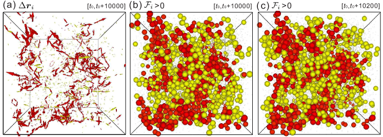
Figure 15: Snapshots in 3D for T=0.24𝑇0.24T=0.24 and N=10000𝑁10000N=10000. (a) Arrows indicate displacements Δ​𝒓i​(t0,t0+10000)Ξ”subscript𝒓𝑖subscript𝑑0subscript𝑑010000\Delta{\mbox{\boldmath$r$}}_{i}(t_{0},t_{0}+10000) with |Δ​𝒓i|>0.3Ξ”subscript𝒓𝑖0.3|\Delta{\mbox{\boldmath$r$}}_{i}|>0.3, whose number is 1818. Particles with β„±i=0subscriptℱ𝑖0{\cal F}_{i}=0 classified into 𝑩𝑩B particles (red) and non-𝑩𝑩B particles (yellow) for time intervals [t0,t0+10000]subscript𝑑0subscript𝑑010000[t_{0},t_{0}+10000] in (b) and [t0,t0+10200]subscript𝑑0subscript𝑑010200[t_{0},t_{0}+10200] in (c). Depicted non-𝑩𝑩B particles are produced by the vibration modes and are fluctuatiing in time, while 𝑩𝑩B particles are not much changed between these two times.
Refer to caption
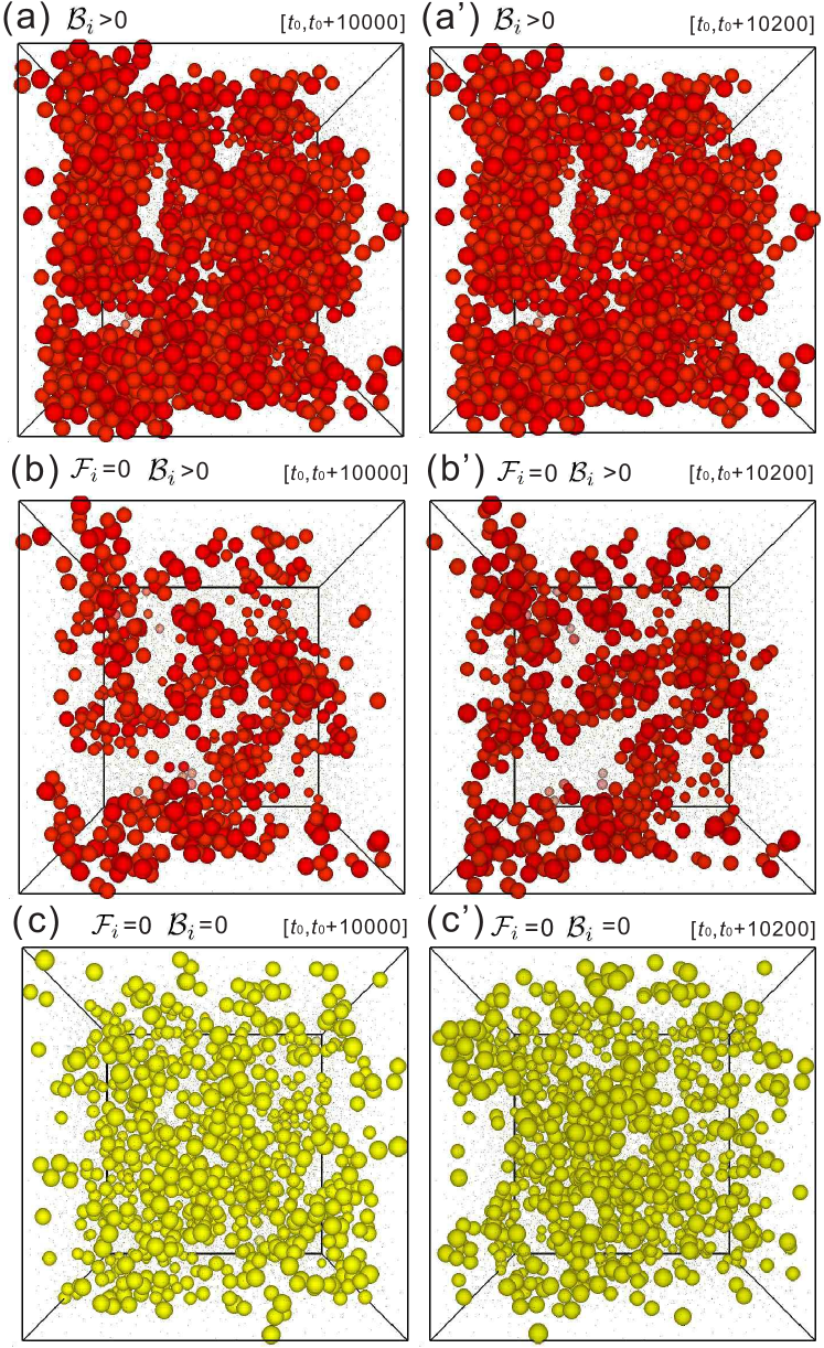
Figure 16: Snapshots using the data in Fig.15 for time intervals [t0,t0+10000]subscript𝑑0subscript𝑑010000[t_{0},t_{0}+10000] (left) and [t0,t0+10200]subscript𝑑0subscript𝑑010200[t_{0},t_{0}+10200] (right). Displayed are particles with ℬi>0subscriptℬ𝑖0{\cal B}_{i}>0 in (a), those with ℬi>0subscriptℬ𝑖0{\cal B}_{i}>0 and β„±i=0subscriptℱ𝑖0{\cal F}_{i}=0 in (b), and those with ℬi=β„±i=0subscriptℬ𝑖subscriptℱ𝑖0{\cal B}_{i}={\cal F}_{i}=0 in (c).

In Fig.15, we give snapshots of the particles at t=10000𝑑10000t=10000 and 10200 for T=0.24𝑇0.24T=0.24 and N=104𝑁superscript104N=10^{4}, where Ο„Ξ±βˆΌ105similar-tosubscriptπœπ›Όsuperscript105\tau_{\alpha}\sim 10^{5}. The system length is L=23.2𝐿23.2L=23.2. Here, the fraction of the 𝑩𝑩B particles is Ο•B​(t)∼0.24similar-tosubscriptitalic-ϕ𝐡𝑑0.24\phi_{B}(t)\sim 0.24 and that with β„±i=0subscriptℱ𝑖0{\cal F}_{i}=0 is Ο•4​(t)∼0.15similar-tosubscriptitalic-Ο•4𝑑0.15\phi_{4}(t)\sim 0.15. In (a), we display the relatively large displacements Δ​𝒓i=𝒓i​(t0+t)βˆ’π’“i​(t0)Ξ”subscript𝒓𝑖subscript𝒓𝑖subscript𝑑0𝑑subscript𝒓𝑖subscript𝑑0\Delta{\mbox{\boldmath$r$}}_{i}={\mbox{\boldmath$r$}}_{i}(t_{0}+t)-{\mbox{\boldmath$r$}}_{i}(t_{0}) with Δ​ri>0.3Ξ”subscriptπ‘Ÿπ‘–0.3\Delta{r}_{i}>0.3. String-like motions are conspicuous Kob ; Sc ; Lacevic ; yo1 , around which collective motions with |Δ​𝒓i|>0.3Ξ”subscript𝒓𝑖0.3|\Delta{\mbox{\boldmath$r$}}_{i}|>0.3 tend to be induced. We also display the particles with β„±i=0subscriptℱ𝑖0{\cal F}_{i}=0 grouping them into 𝑩𝑩B particles (in red) and non-𝑩𝑩B particles (in yellow) in time intervals [t0,t0+10000]subscript𝑑0subscript𝑑010000[t_{0},t_{0}+10000] in (b) and [t0,t0+10200]subscript𝑑0subscript𝑑010200[t_{0},t_{0}+10200] in (c).

In Fig.16, we display the 𝑩𝑩B particles in (a) and (a’), the 𝑩𝑩B particles with β„±i=0subscriptℱ𝑖0{\cal F}_{i}=0 in (b) and (b’), and the non-𝑩𝑩B particles with β„±i=0subscriptℱ𝑖0{\cal F}_{i}=0 in (c) and (c’) for t=10000𝑑10000t=10000 in the left and 10200 in the right. We use the same data as in Fig.15. We can see that the 𝑩𝑩B particles little change, but the non-𝑩𝑩B particles much change in a time interval of 200. The aggregates of the 𝑩𝑩B particles have grown from the strings in (a) in Fig.15. The number of the total 𝑩𝑩B particles (in the top panels) is considerably larger than that of the 𝑩𝑩B particles with β„±i=0subscriptℱ𝑖0{\cal F}_{i}=0 (in the midde panels), which are 2351 and 641, respectively, at t=10000𝑑10000t=10000. This is because the particles surrounding each string can have broken bonds without their long-disance motions.

Table III gives the numbers of the particles with (a) ℬi>0subscriptℬ𝑖0{\cal B}_{i}>0, (b) ℬi>0subscriptℬ𝑖0{\cal B}_{i}>0 and β„±i=0subscriptℱ𝑖0{\cal F}_{i}=0, (c) ℬi=β„±i=0subscriptℬ𝑖subscriptℱ𝑖0{\cal B}_{i}={\cal F}_{i}=0, and (d) Δ​ri>0.3Ξ”subscriptπ‘Ÿπ‘–0.3\Delta r_{i}>0.3 in the two snapshots in Figs.15 and 16. Also given in the last line are those of the particles commonly depicted in the consecutive snapshots. On the other hand, Table IV presents the numbers of the 𝑩𝑩B and non-𝑩𝑩B particles at t=10200𝑑10200t=10200 for (a) Δ​ri>0.3Ξ”subscriptπ‘Ÿπ‘–0.3{\Delta r}_{i}>0.3 and β„±i=0subscriptℱ𝑖0{\cal F}_{i}=0, (b) Δ​ri>0.3Ξ”subscriptπ‘Ÿπ‘–0.3{\Delta r}_{i}>0.3 and β„±i=1subscriptℱ𝑖1{\cal F}_{i}=1, and (c) Δ​ri<0.3Ξ”subscriptπ‘Ÿπ‘–0.3{\Delta r}_{i}<0.3 and β„±i=1subscriptℱ𝑖1{\cal F}_{i}=1. Conspicuous features are as follows. (i) About 50%percent5050\% particles with Δ​r>0.3Ξ”π‘Ÿ0.3\Delta r>0.3 change into those with Δ​ri<0.3Ξ”subscriptπ‘Ÿπ‘–0.3\Delta r_{i}<0.3 and vice versa in a short time interval of 200. Only 30%percent3030\% of the non-𝑩𝑩B particle are common in the two consecutive snapshots. (ii) About 60%percent6060\% of the 𝑩𝑩B particles satisfy Δ​ri<0.3Ξ”subscriptπ‘Ÿπ‘–0.3\Delta r_{i}<0.3 and β„±i=0subscriptℱ𝑖0{\cal F}_{i}=0. (The corresponding percentage is about 15%percent1515\% in 2D in Table II.) This is because of the larger coordination number or the larger bonded particles around each particle in 3D. That is, there are about 10 bonded particles around a particle which has participated in a string-like motion and moved over a molecular distance. (iii) The particles with Δ​ri>0.3Ξ”subscriptπ‘Ÿπ‘–0.3\Delta r_{i}>0.3 and β„±i=1subscriptℱ𝑖1{\cal F}_{i}=1 amount to 366366366 and their fraction in those with Δ​ri>0.3Ξ”subscriptπ‘Ÿπ‘–0.3\Delta r_{i}>0.3 is about 0.20.20.2. This means that the distinct part is negligible as compared to the self part in β„±isubscriptℱ𝑖{\cal{F}}_{i} in Eq.(4.2), in accord with the calculation by La ̌ceviΔ‡ et al.Lacevic . (iv) Among 366366366 particles with Δ​ri>0.3Ξ”subscriptπ‘Ÿπ‘–0.3\Delta r_{i}>0.3 and β„±i=1subscriptℱ𝑖1{\cal F}_{i}=1, most of them (339) are 𝑩𝑩B particles.

Table 3: Particle numbers in Figs.15 and 16 at t=10000𝑑10000t=10000 and 10200 for N=104𝑁superscript104N=10^{4} in 3D.
t𝑑t ℬ>0ℬ0{\cal B}>0~{}~{} ℬ>0ℬ0{\cal B}>0,β„±=0β„±0{\cal F}=0 ℬ=β„±=0ℬℱ0{\cal B}={\cal F}=0 Δ​r>0.3Ξ”π‘Ÿ0.3\Delta r>0.3
100001000010000 2351 641 811 1818
102001020010200 2393 675 898 1943
common 2094 400 268 980
Table 4: Numbers of non-𝑩𝑩B and 𝑩𝑩B particles for three categories at t=10000𝑑10000t=10000 for N=104𝑁superscript104N=10^{4} in 3D in Figs.13 and 14.
Δ​r>0.3Ξ”π‘Ÿ0.3{\Delta r}>0.3 Δ​r>0.3Ξ”π‘Ÿ0.3{\Delta r}>0.3 Δ​r<0.3Ξ”π‘Ÿ0.3{\Delta r}<0.3
β„±=0β„±0{\cal F}=0 β„±=1β„±1{\cal F}=1 β„±=1β„±1{\cal F}=1 total
ℬ=0ℬ0{\cal B}=0 811 27 6811 7649
ℬ>0ℬ0{\cal B}>0 641 339 1371 2351
total 1452 366 8182 10000

VII Summary and remarks

We have examined the dynamic heterogeneity of glassy particle systems in the bond-breakage scheme yo ; yo1 and in the four-point scheme Lacevic . The former treats the irreversible configuration changes, while in the latter also included are the reversible particle displacements due to the low-frequency vibrational modes. These two kinds of motions are both highly heterogeneous in glassy states.

Our main results are as follows.
(i) In Sec.III, we have generalized the bond breakage theory yo ; yo1 to define the broken bond number ℬi​(t0,t1)subscriptℬ𝑖subscript𝑑0subscript𝑑1{\cal B}_{i}(t_{0},t_{1}), the fractions of the particles with kπ‘˜k broken bonds Ο•b​(t,k)subscriptitalic-Ο•π‘π‘‘π‘˜\phi_{b}(t,k), the correlation function Gb​(r,t)subscriptπΊπ‘π‘Ÿπ‘‘G_{b}(r,t), the structure factor Sb​(q,t)subscriptπ‘†π‘π‘žπ‘‘S_{b}(q,t), and the susceptibility Ο‡b​(t)subscriptπœ’π‘π‘‘\chi_{b}(t) in Eqs.(3.12), (3.14), and (3.19)-(3.21). We have defined the bond-breakage time Ο„bsubscriptπœπ‘\tau_{b} in Eq.(3.4) and the bond-preserving time Ο„b​psubscriptπœπ‘π‘\tau_{bp} in Eq.(3.16) in addition to the relaxation time ταsubscriptπœπ›Ό\tau_{\alpha} from Fs​(q,t)subscriptπΉπ‘ π‘žπ‘‘F_{s}(q,t) in Eq.(3.6). In Fig.3, Ο‡b​(t)subscriptπœ’π‘π‘‘\chi_{b}(t) exhibits a maximum as a function of t𝑑t, yielding the maximization time tbmaxsuperscriptsubscript𝑑𝑏maxt_{b}^{\rm max}, while the Ornstein-Zernike fitting of Sb​(q,tbmax)subscriptπ‘†π‘π‘žsuperscriptsubscript𝑑𝑏maxS_{b}(q,t_{b}^{\rm max}) yields ΞΎb=ΞΎb​(tbmax)subscriptπœ‰π‘subscriptπœ‰π‘superscriptsubscript𝑑𝑏max\xi_{b}=\xi_{b}(t_{b}^{\rm max}) in Fig.4. These quantities are nearly independent of the system size as long as 1β‰ͺΞΎbβ‰ͺLmuch-less-than1subscriptπœ‰π‘much-less-than𝐿1\ll\xi_{b}\ll L.
(ii) In Sec.IV, we have discussed the four-point theory, where the overlap function w​(r)π‘€π‘Ÿw(r) in Eq.(4.3) defines the initial circles (spheres) in 2D (3D). The overlap number β„±i​(t0,t1)subscriptℱ𝑖subscript𝑑0subscript𝑑1{\cal F}_{i}(t_{0},t_{1}) in Eq.(4.2) determines the correlation function G4​(r,t)subscript𝐺4π‘Ÿπ‘‘G_{4}(r,t), the structure factor S4​(q,t)subscript𝑆4π‘žπ‘‘S_{4}(q,t), and the susceptibility Ο‡4​(t)subscriptπœ’4𝑑\chi_{4}(t) in Eqs.(4.12)-(4.14). Maximization of Ο‡4​(t)subscriptπœ’4𝑑\chi_{4}(t) with respect to t𝑑t yields the characteristic time t4maxsuperscriptsubscript𝑑4maxt_{4}^{\rm max}. We have shown that the nonoverlap motions from the initial circles stem from the thermal excitation of the low-frequency vibrational modes and the escape jumps from temporary cages as in Figs.5, 6, 11, and 13. The thermal collective motions appear from the initial stage (t≳10)t\gtrsim 10) as in Fig.7, while the jump motions emerge very slowly. The maximization procedure of Ο‡4​(t)subscriptπœ’4𝑑\chi_{4}(t) with respect to the overlap length Lacevic is to maximize the contribution from the thermal collective motions to Ο‡4​(t)subscriptπœ’4𝑑\chi_{4}(t). In 2D, the system-size dependence of the four-point correlations is strong at long wavelengths even for ΞΎ4β‰ͺLmuch-less-thansubscriptπœ‰4𝐿\xi_{4}\ll L.
(iii) In Sec.V, we have compared the relaxation times Ο„bsubscriptπœπ‘\tau_{b}, Ο„p​bsubscriptπœπ‘π‘\tau_{pb}, ταsubscriptπœπ›Ό\tau_{\alpha}, tbmaxsuperscriptsubscript𝑑𝑏maxt_{b}^{\rm max}, and t4maxsuperscriptsubscript𝑑4maxt_{4}^{\rm max} in Fig.12 to obtain the sequence (5.1), where τα(∼t4max)annotatedsubscriptπœπ›Όsimilar-toabsentsuperscriptsubscript𝑑4max\tau_{\alpha}(\sim t_{4}^{\rm max}) is considerably shorter than Ο„bsubscriptπœπ‘\tau_{b}. Next we have presented snapshots of the displacements, ℬisubscriptℬ𝑖{\cal B}_{i}, and β„±isubscriptℱ𝑖{\cal F}_{i} at t=104𝑑superscript104t=10^{4} for N=4000𝑁4000N=4000 with marked large-scale heterogeneities in Fig.13. We have grouped the particles with β„±i=0subscriptℱ𝑖0{\cal F}_{i}=0 into 𝑩𝑩B and non-𝑩𝑩B particles, where they are those with and without broken bonds, respectively. The patterns of the 𝑩𝑩B particles with β„±i=0subscriptℱ𝑖0{\cal F}_{i}=0 closely resemble those of the total 𝑩𝑩B particles. The non-𝑩𝑩B particles with β„±i=0subscriptℱ𝑖0{\cal F}_{i}=0 arise from the low-frequency vibration modes undergoing relatively rapid temporal variations, as can be seen in the inset of Fig.6 and in Fig.14.
(iv) Also in 3D, the four-point correlations arise from the thermal collective motions with ℬi=0subscriptℬ𝑖0{\cal B}_{i}=0 and the bond-breakage motions with ℬiβ‰₯1subscriptℬ𝑖1{\cal B}_{i}\geq 1 as in Figs.15 and 16. As a charcteristic feature in 3D, Table IV shows that about 60%percent6060\% of the 𝑩𝑩B paricles satisfy Δ​ri<0.3Ξ”subscriptπ‘Ÿπ‘–0.3\Delta r_{i}<0.3 and β„±i=1subscriptℱ𝑖1{\cal F}_{i}=1. These particles suround the particles which have undergone string-like motions.

We make some remarks in the following.
(1) The heterogeneity exhibited by the low-frequency vibration modes still remains largely unexplored Ruocco ; Shintani ; Liu ; Reichman ; Barrat ; Bonn ; Br . In future work, we should examine how it depends on the size ratio and the composition Hama ; Jack ; Shiba .
(2) The vibration modes determine the plateaus of the time-correlation function Fs​(q,t)subscriptπΉπ‘ π‘žπ‘‘F_{s}(q,t) in Eq.(3.5) and the mean square displacement M​(t)𝑀𝑑M(t) in Eq.(A4), resulting in significant system-size effects finite ; Kim . They also give rise to the system-size dependence of the four-point structure S4​(q,t)subscript𝑆4π‘žπ‘‘S_{4}(q,t) at small qπ‘žq in (b) of Fig.10. Our present analysis is mostly for 2D, but Eqs.(A2) and (A8) provide one possible sourse of the finite size effect in 3D.
(3) We also comment on the effect of a thermostat, which was used only in preparing the initial states. We have found that a thermostat can strongly affect the low-frequency vibration modes (not shown in this paper). For example, the second peak of Ο‡4​(t)subscriptπœ’4𝑑\chi_{4}(t) at tβ‰…L/2​cβŸ‚π‘‘πΏ2subscript𝑐perpendicular-tot\cong L/2c_{\perp} for T≀0.80𝑇0.80T\leq 0.80 in Fig.9 disappeared in the presence of a thermostat, presumably because it effectively increases the acoustic damping.

Acknowledgements.
This work was supported by Grant-in-Aid for Scientific Research from the Ministry of Education, Culture, Sports, Science and Technology of Japan. T. K. was supported by the Japan Society for Promotion of Science. The authors would like to thank Ryoichi Yamamoto, Kunimasa Miyazaki, Shinichi Sasa, and Kang Kim for informative discussions. The numerical calculations were carried out on SR16000 at YITP in Kyoto University and Altix ICE 8400EX at ISSP in University of Tokyo.

Appendix: Thermal positional fluctuations and finite size effect

In solids, the vibration modes give rise to the thermal fluctuations of the particle displacements 𝒖i​(t)=𝒓i​(t)βˆ’π’“Β―isubscript𝒖𝑖𝑑subscript𝒓𝑖𝑑subscript¯𝒓𝑖{\mbox{\boldmath$u$}}_{i}(t)={\mbox{\boldmath$r$}}_{i}(t)-{\bar{\mbox{\boldmath$r$}}}_{i} with 𝒓¯isubscript¯𝒓𝑖{\bar{\mbox{\boldmath$r$}}}_{i} being the time-averaged positions. In our theory, we may define 𝒓¯isubscript¯𝒓𝑖{\bar{\mbox{\boldmath$r$}}}_{i} on timescales shorter than the bond-preserving time Ο„bpsubscript𝜏bp\tau_{\rm bp} in Eq.(3.16). The contributions from the large-scale modes may be calculated using the classical linear elasticity theory, which should be valid at sufficiently long wavelengths even in glass Barrat .

In 2D, we may expresss the displacement variance ⟨|𝒖|2⟩=βˆ‘i⟨|𝒖i|2⟩/Ndelimited-⟨⟩superscript𝒖2subscript𝑖delimited-⟨⟩superscriptsubscript𝒖𝑖2𝑁\langle{|{\mbox{\boldmath$u$}}|^{2}}\rangle=\sum_{i}\langle{|{\mbox{\boldmath$u$}}_{i}|^{2}}\rangle/N as in Eqs.(4.6) and (4.7). For 2D solids Janco , use has been made of the relation,

⟨|𝒖i​(t)βˆ’π’–j​(t)|2⟩=2​C1​ln⁑(ri​j/a0),delimited-⟨⟩superscriptsubscript𝒖𝑖𝑑subscript𝒖𝑗𝑑22subscript𝐢1subscriptπ‘Ÿπ‘–π‘—subscriptπ‘Ž0\langle{|{\mbox{\boldmath$u$}}_{i}(t)-{\mbox{\boldmath$u$}}_{j}(t)|^{2}}\rangle=2C_{1}\ln(r_{ij}/a_{0}), (A1)

where C1subscript𝐢1C_{1} is given in E.(4.7), ri​jsubscriptπ‘Ÿπ‘–π‘—r_{ij} is the distance between particles i𝑖i and j𝑗j, and a0subscriptπ‘Ž0a_{0} is a microscopic length. Thus, Eq.(A1) represents the anomalous long-range correlation in 2D solids. These expressions folllow if the discrete sums over the long-wavelength vibration modes (βˆ‘π’’|𝒒|βˆ’2subscript𝒒superscript𝒒2\sum_{\mbox{\boldmath$q$}}|{\mbox{\boldmath$q$}}|^{-2}) are replaced by the wave-number integral (βˆ«π‘‘q​qdβˆ’3differential-dπ‘žsuperscriptπ‘žπ‘‘3\int dqq^{d-3}). In 3D, there is no long-wavelength divergence, but the lower bound of the wave number (∝Lβˆ’1proportional-toabsentsuperscript𝐿1\propto L^{-1}) yields the following L𝐿L dependence,

⟨|𝒖|2⟩=D0βˆ’D1/L,delimited-⟨⟩superscript𝒖2subscript𝐷0subscript𝐷1𝐿\langle{|{\mbox{\boldmath$u$}}|^{2}}\rangle=D_{0}-D_{1}/L, (A2)

where D0subscript𝐷0D_{0} and D1subscript𝐷1D_{1} are functions of T𝑇T. If we perform the corresponding discrete summation over the modes under the periodic boundary condition, we obtain

D1=0.21​kB​T​(2ΞΌ+1K+4​μ/3).subscript𝐷10.21subscriptπ‘˜π΅π‘‡2πœ‡1𝐾4πœ‡3D_{1}=0.21{k_{B}T}\bigg{(}\frac{2}{\mu}+\frac{1}{K+4\mu/3}\bigg{)}. (A3)

For tβ‰ͺΟ„b​pmuch-less-than𝑑subscriptπœπ‘π‘t\ll\tau_{bp}, we may set 𝒓i​(t0)βˆ’π’“i​(t0+t)=𝒖i​(t0)βˆ’π’–i​(t0+t)subscript𝒓𝑖subscript𝑑0subscript𝒓𝑖subscript𝑑0𝑑subscript𝒖𝑖subscript𝑑0subscript𝒖𝑖subscript𝑑0𝑑{\mbox{\boldmath$r$}}_{i}(t_{0})-{\mbox{\boldmath$r$}}_{i}(t_{0}+t)={\mbox{\boldmath$u$}}_{i}(t_{0})-{\mbox{\boldmath$u$}}_{i}(t_{0}+t) by neglecting the configuration changes. The mean square displacement M​(t)𝑀𝑑M(t) is written as

M​(t)𝑀𝑑\displaystyle M(t) =\displaystyle= βˆ‘i⟨|𝒓i​(t0)βˆ’π’“i​(t0+t)|2⟩/Nsubscript𝑖delimited-⟨⟩superscriptsubscript𝒓𝑖subscript𝑑0subscript𝒓𝑖subscript𝑑0𝑑2𝑁\displaystyle\sum_{i}\langle{|{\mbox{\boldmath$r$}}_{i}(t_{0})-{\mbox{\boldmath$r$}}_{i}(t_{0}+t)|^{2}}\rangle/N (A4)
β‰…\displaystyle\cong βˆ‘i⟨|𝒖i​(t0)βˆ’π’–i​(t0+t)|2⟩/N.subscript𝑖delimited-⟨⟩superscriptsubscript𝒖𝑖subscript𝑑0subscript𝒖𝑖subscript𝑑0𝑑2𝑁\displaystyle\sum_{i}\langle{|{\mbox{\boldmath$u$}}_{i}(t_{0})-{\mbox{\boldmath$u$}}_{i}(t_{0}+t)|^{2}}\rangle/N.

If the cross correlation βˆ‘iβŸ¨π’–i​(t0+t)⋅𝒖i​(t0)⟩/Nsubscript𝑖delimited-βŸ¨βŸ©β‹…subscript𝒖𝑖subscript𝑑0𝑑subscript𝒖𝑖subscript𝑑0𝑁\sum_{i}\langle{{\mbox{\boldmath$u$}}_{i}(t_{0}+t)\cdot{\mbox{\boldmath$u$}}_{i}(t_{0})}\rangle/N decays to zero due to the acoustic damping before the α𝛼\alpha relaxation, a well-defined pleteau Mpsubscript𝑀pM_{\rm p} appears in M​(t)𝑀𝑑M(t) with

M​(t)β‰…Mp=2β€‹βŸ¨|𝒖|2⟩,𝑀𝑑subscript𝑀p2delimited-⟨⟩superscript𝒖2M(t)\cong M_{\rm p}=2\langle{|{\mbox{\boldmath$u$}}|^{2}}\rangle, (A5)

for 1β‰ͺtβ‰ͺΟ„b​pmuch-less-than1𝑑much-less-thansubscriptπœπ‘π‘1\ll t\ll\tau_{bp} as already given in Eq.(4.6).

The time correlation function Fs​(q,t)subscriptπΉπ‘ π‘žπ‘‘F_{s}(q,t) in Eq.(3.5) also assumes a well-defined plateau value fp=fp​(T,N)subscript𝑓psubscript𝑓p𝑇𝑁f_{\rm p}=f_{\rm p}(T,N) at low T𝑇T. For the Gaussian distribution of 𝒖isubscript𝒖𝑖{\mbox{\boldmath$u$}}_{i}, we have Hansen

fpβ‰…exp⁑[βˆ’q2​Mp/2​d]=exp⁑[βˆ’q2β€‹βŸ¨|𝒖|2⟩/d],subscript𝑓psuperscriptπ‘ž2subscript𝑀p2𝑑superscriptπ‘ž2delimited-⟨⟩superscript𝒖2𝑑f_{\rm p}\cong\exp[-q^{2}M_{\rm p}/2d]=\exp[-q^{2}\langle{|{\mbox{\boldmath$u$}}|^{2}}\rangle/d], (A6)

If the structural relaxation time ταsubscriptπœπ›Ό\tau_{\alpha} is defined by Eq.(3.6), its dependence on N(∝N1/d)annotated𝑁proportional-toabsentsuperscript𝑁1𝑑N(\propto N^{1/d}) can arise from Eq.(4.6) in 2D and from Eq.(A2) in 3D.

For 2D, fpsubscript𝑓pf_{\rm p} depends on N𝑁N as

fp∝Lβˆ’q2​C1/2∝Nβˆ’q2​C1/4.proportional-tosubscript𝑓psuperscript𝐿superscriptπ‘ž2subscript𝐢12proportional-tosuperscript𝑁superscriptπ‘ž2subscript𝐢14f_{\rm p}\propto L^{-q^{2}C_{1}/2}\propto N^{-q^{2}C_{1}/4}. (A7)

For T=0.56𝑇0.56T=0.56 and q=2β€‹Ο€π‘ž2πœ‹q=2\pi, our numerical analysis gives fp=0.6subscript𝑓p0.6f_{\rm p}=0.6 for N=4000𝑁4000N=4000 in Fig.1 and fp=0.5subscript𝑓p0.5f_{\rm p}=0.5 for N=64000𝑁64000N=64000. The ratio of these two values 0.6/0.5=1.20.60.51.20.6/0.5=1.2 is close to the theoretical ratio 16q2​C1/4=1.17superscript16superscriptπ‘ž2subscript𝐢141.1716^{q^{2}C_{1}/4}=1.17 from Eq.(A7).

For 3D, Eqs.(A2), (A5), and (A6) yield

fp​(T,N)/fp​(T,∞)=exp⁑[Bf​Nβˆ’1/3].subscript𝑓p𝑇𝑁subscript𝑓p𝑇subscript𝐡𝑓superscript𝑁13f_{\rm p}(T,N)/f_{\rm p}(T,\infty)=\exp[B_{f}N^{-1/3}]. (A8)

Under the periodic boundary condition, Eq.(A3) gives

Bfβ‰…0.14​q2​kB​T​n1/3/ΞΌ,subscript𝐡𝑓0.14superscriptπ‘ž2subscriptπ‘˜π΅π‘‡superscript𝑛13πœ‡B_{f}\cong 0.14q^{2}k_{B}Tn^{1/3}/\mu, (A9)

where K𝐾K is assumed to be considerably larger than ΞΌπœ‡\mu. Kim and Yamamoto Kim studied the finite size effect using the soft-core potential for N=108,103𝑁108superscript103N=108,10^{3}, and 104superscript10410^{4} in 3D. Their data of Fs​(q,t)subscriptπΉπ‘ π‘žπ‘‘F_{s}(q,t) at t=10𝑑10t=10 for q=2β€‹Ο€π‘ž2πœ‹q=2\pi and T=0.267𝑇0.267T=0.267 may be approximately fitted to the form ∝exp⁑[0.25​Nβˆ’1/3]proportional-toabsent0.25superscript𝑁13\propto\exp[0.25N^{-1/3}], while Eqs.(A8) and (A9) give fp∝exp⁑[0.29​Nβˆ’1/3]proportional-tosubscript𝑓p0.29superscript𝑁13f_{\rm p}\propto\exp[0.29N^{-1/3}] (where we obtain ΞΌ=5πœ‡5\mu=5 from the stress-strain relation).

References

  • (1) K. Binder and W. Kob, Glassy Materials and Disordered Solids (World Scientific, Singapore, 2005).
  • (2) G. Adam and J. H. Gibbs, J. Chem. Phys. 43, 139 (1965).
  • (3) H. Sillescu, J. Non-Cryst. Solids 243, 81 (1999).
  • (4) M. D. Ediger, Annu. Rev. Phys. Chem. 51, 99 (2000).
  • (5) L. Berthier, G. Biroli, J.-P. Bouchaud, L. Cipelletti, and W. van Saarloos, Dynamical Heterogeneities in Glasses, Colloids, and Granular Media (Oxford University Press, Oxford, 2011).
  • (6) K. Maeda and S. Takeuchi, Phys. Stat. Sol. 49, 685 (1978); Philos. Mag. 44, 643 (1981).
  • (7) D. Srolovitz, V. Vitek, T. Egami, Acta. Metall. 31, 335 (1983).
  • (8) D. Deng, A.S. Argon, and S. Yip, Phil. Trans. R. Soc. Lond. A, 329, 595, 613 (1989).
  • (9) M. M. Hurley and P. Harrowell, Phys. Rev. E 52, 1694 (1995).
  • (10) D.N. Perera and P. Harrowell, Phys. Rev. Lett. 81, 120 (1998); J. Chem. Phys. 111, 5441 (1999).
  • (11) T. Muranaka and Y. Hiwatari, Phys. Rev. E 51, R2735 (1995).
  • (12) Y. Hiwatari and T. Muranaka, J. Non-Cryst. Solids 235-237, 19 (1998). Figure 6 of their paper is similar to (a) of Fig.7 in the present paper.
  • (13) R. Yamamoto and A. Onuki, J. Phys. Soc. Jpn., 66, 2545 (1997).
  • (14) R. Yamamoto and A. Onuki, Phys. Rev. E 58, 3515 (1998). See Fig.16 of this paper for the relation between Ο„bsubscriptπœπ‘\tau_{b} and ταsubscriptπœπ›Ό\tau_{\alpha}; R. Yamamoto and A. Onuki, J. Phys.: Condens. Matter 29, 6323 (2000).
  • (15) R. Yamamoto and A. Onuki, Phys. Rev. Lett. 81, 54915 (1998).
  • (16) W. Kob, C. Donati, S. J. Plimpton, P. H. Poole, and S. C. Glotzer, Phys. Rev. Lett. 79, 2827 (1997); C. Donati, J. F. Douglas, W. Kob, S. J. Plimpton, P. H. Poole, and S. C. Glotzer, Phys. Rev. Lett. 80, 2338 (1998); C. Donati, S. C. Glotzer, P. H. Poole, W. Kob, and S. J. Plimpton, Phys. Rev. E 60, 3107 (1999).
  • (17) D.N. Perera, J. Phys.: Condens. Matter 10, 10115 (1998).
  • (18) B. Doliwa and A. Heuer, Phys. Rev. E 61, 6898 (2000); J. Non-Cryst. Solids 307-310, 32 (2002).
  • (19) D. Chandler, J. P. Garrahan, R. L. Jack, L. Maibaum, and A. C. Pan, Phys. Rev. E 74, 051501 (2006).
  • (20) G. Biroli, J.-P. Bouchaud, K. Miyazaki, and D.R. Reichman, Phys. Rev. Lett. 97, 195701 (2006).
  • (21) R. Candelier, A. Widmer-Cooper, J. K. Kummerfeld, O. Dauchot, G. Biroli, P. Harrowell, and D. R. Reichman, Phys. Rev. Lett. 105, 135702 (2010).
  • (22) T. Kawasaki, T. Araki, and H. Tanaka, Phys. Rev. Lett. 99, 215701 (2007).
  • (23) N. La ̌ceviΔ‡, F. W. Starr, T. B. Schroder, and S. C. Glotzer, J. Chem. Phys. 119, 7372 (2003).
  • (24) L. Berthier, G. Biroli, J.-P. Bouchaud, L. Cipelletti, D. E. Masri, D. L fHote, F. Ladieu, and M. Pierno, Science 310, 1797 (2005).
  • (25) L. Berthier, G. Biroli, J.-P. Bouchaud, W. Kob, K. Miyazaki, and D. R. Reichman, J. Chem. Phys. 126, 184503 (2007); ibid. 126,184504 (2007).
  • (26) D. Chandler, J. P. Garrahan, R. L. Jack, L. Maibaum, and A. C. Pan, Phys. Rev. E 74, 051501 (2006).
  • (27) S. Karmakar, C. Dasgupta, and S. Sastry, Phys. Rev. Lett. 105, 015701 (2010); ibid. 105, 019801 (2010).
  • (28) E. Flenner, M. Zhang, and G. Szamel, Phys. Rev. E 83, 051501 (2011).
  • (29) H. Mizuno and R. Yamamoto, Phys. Rev. E 84, 011506 (2011).
  • (30) A. Furukawa and H. Tanaka, Phys. Rev. E 84, 061503 (2011).
  • (31) H. R. Schober and B. B. Laird, Phys. Rev. B 44, 6746 (1991).
  • (32) W. Schirmacher, G. Diezemann, and C. Ganter, Phys. Rev. Lett. 81, 136 (1998).
  • (33) H. R. Schober, C. Oligschleger, and B. B. Laird, J. Non-Cryst. Solids 156, 965 (1993); C. Oligschleger and H. R. Schober, Phys. Rev. B 59, 811 (1999).
  • (34) L. Angelani, M. Montagna, G. Ruocco, and G. Viliani, Phys. Rev. Lett. 84, 4874 (2000).
  • (35) A. Tanguy, J. P. Wittmer, F. Le´´e\acute{\rm e}onforte, and J.-L. Barrat, Phys. Rev. B 66, 174205 (2002); F. Leonforte, R. Boissiere, A. Tanguy, J. P. Wittmer, and J.-L. Barrat, Phys. Rev. B 72, 224206 (2005); F. Le´´e\acute{\rm e}onforte, A. Tanguy, J. P. Wittmer, and J.-L. Barrat, Phys. Rev. Lett. 97, 055501 (2006).
  • (36) H. R. Schober and G. Ruocco, Philos. Mag. 84, 1361 (2004).
  • (37) H. Shintani and H. Tanaka, Nature Matterials 7, 870 (2008).
  • (38) C. Brito and M. Wyart, J. Chem. Phys. 131, 024504 (2009).
  • (39) A. Widmer-Cooper, H. Perry, P. Harrowell Cand D. R. Reichman, Nature Physics 4, 711 (2008); J. Chem. Phys. 131, 194508 (2009).
  • (40) A. Ghosh, V.K. Chikkadi, P. Schall, J. Kurchan, and D. Bonn, Phys. Rev. Lett. 104, 248305 (2010).
  • (41) K. Chen, W. G. Ellenbroek, Z. Zhang, D. T. N. Chen, P. J. Yunker, S. Henkes, C. Brito, O. Dauchot, W. van Saarloos, A. J. Liu, and A. G. Yodh, Phys. Rev. Lett. 105, 025501 (2010).
  • (42) K. Chen, M. L. Manning, P. J. Yunker, W. G. Ellenbroek, Z. Zhang, A. J. Liu, and A. G. Yodh, Phys. Rev. Lett. 107, 108301 (2011).
  • (43) K. Vollmayr-Lee, W. Kob, K. Binder, and A. Zippelius, J. Chem. Phys. 116, 5158 (2002).
  • (44) A. Widmer-Cooper and P. Harrowell, Phys. Rev. Lett. 96, 185701 (2006).
  • (45) T. Hamanaka and A. Onuki, Phys. Rev. E 74, 011506 (2006); ibid. 75, 041503 (2007).
  • (46) H. Zhang, D. J. Srolovitz, J. F. Douglas, and J. A. Warren, Phys. Rev. B 74, 115404 (2006); PNAS 106 May 12, 7735 (2009).
  • (47) H. Shiba and A. Onuki, Phys. Rev. E 81, 051501 (2010).
  • (48) M. Tsamados, A. Tanguy, C. Goldenberg, and J.-L. Barrat, Phys. Rev. E 80, 026112 (2009).
  • (49) K. Yoshimoto, T. S. Jain, K. Van Workum, P. F. Nealey, and J. J. de Pablo, Phys. Rev. Lett. 93, 175501 (2004).
  • (50) Y. Shi, M. B. Katz, H. Li, and M. L. Falk, Phys. Rev. Lett. 98, 185505 (2007); A. Lemaitre and C. Caroli, Phys. Rev. E 76, 036104 (2007); A. Furukawa, K. Kim, S. Saito, and H. Tanaka, Phys. Rev. Lett. 102, 016001 (2009).
  • (51) M. L. Manning and A. J. Liu, Phys. Rev. Lett. 107, 108302 (2011).
  • (52) E. Rabani, J. D. Gezelter, and B. J. Berne, J. Chem. Phys. 107, 6867 (1997); Phys. Rev. Lett. 82, 3649 (1999).
  • (53) A. R. Abate and D. J. Durian, Phys. Rev. E 74, 031308 (2006)
  • (54) B. Jancovici, Phys. Rev. Lett. 19, 20 (1967); Y. Imry and L. Gunther, Phys. Rev. B, 3, 3939 (1971); D. R. Nelson and B. I. Halperin, Phys. Rev. B, 19, 2457 (1979).
  • (55) In our simulation, the transverse and longitudinal sound velocities are given by cβŸ‚=(ΞΌ/ρ)1/2β‰…4.1subscript𝑐perpendicular-tosuperscriptπœ‡πœŒ124.1c_{\perp}=({\mu/\rho})^{1/2}\cong 4.1 and cβˆ₯=[(K+ΞΌ)/ρ]1/2β‰…8.9subscript𝑐parallel-tosuperscriptdelimited-[]πΎπœ‡πœŒ128.9c_{\parallel}=[(K+\mu)/\rho]^{1/2}\cong 8.9 in units of Οƒ1/Ο„0subscript𝜎1subscript𝜏0\sigma_{1}/\tau_{0} at T=0.56𝑇0.56T=0.56 in 2D, where ρ=1.06​m1​σ1βˆ’2𝜌1.06subscriptπ‘š1superscriptsubscript𝜎12\rho=1.06m_{1}\sigma_{1}^{-2} is the average mass density.
  • (56) T. Muranaka and Y. Hiwatari, Mol. Simul. 16, 387 (1996); J. Horbach, W. Kob, K. Binder, and C.A. Angell, Phys. Rev. E 54, R5897 (1996).
  • (57) K. Kim and R. Yamamoto, Phys. Rev. E 61, R41 (2000).
  • (58) O. Dauchot, G. Marty, and G. Biroli, Phys. Rev. Lett. 95, 265701 (2005).
  • (59) G. Pastore, B. Bernu, J. P. Hansen, and Y. Hiwatari, Phys. Rev. A 38, 454 (1988).