THE DOMINANCE OF NEUTRINO-DRIVEN CONVECTION IN CORE-COLLAPSE SUPERNOVAE
Abstract
Multi-dimensional instabilities have become an important ingredient in core-collapse supernova (CCSN) theory. Therefore, it is necessary to understand the driving mechanism of the dominant instability. We compare our parameterized three-dimensional CCSN simulations with other buoyancy-driven simulations and propose scaling relations for neutrino-driven convection. Through these comparisons, we infer that buoyancy-driven convection dominates post-shock turbulence in our simulations. In support of this inference, we present four major results. First, the convective fluxes and kinetic energies in the neutrino-heated region are consistent with expectations of buoyancy-driven convection. Second, the convective flux is positive where buoyancy actively drives convection, and the radial and tangential components of the kinetic energy are in rough equipartition (i.e. ). Both results are natural consequences of buoyancy-driven convection, and are commonly observed in simulations of convection. Third, buoyant driving is balanced by turbulent dissipation. Fourth, the convective luminosity and turbulent dissipation scale with the driving neutrino power. In all, these four results suggest that in neutrino-driven explosions, the multi-dimensional motions are consistent with neutrino-driven convection.
Subject headings:
convection — hydrodynamics — instabilities — methods:analytical — methods: numerical — shock waves — supernovae: general — turbulence1. Introduction
The explosive death of massive stars, in particular core-collapse supernovae (CCSNe), are some of the most energetic explosions in the Universe, and, as such, are fundamental to a wide range of other astrophysical phenomena. To highlight a few important examples, CCSNe are a major site for nucleosynthesis, mark the birth of neutron stars and black holes, and are major contributors to galactic dynamics and star formation. Despite their importance, understanding the mechanism remains an important unsolved problem. Whatever the mechanism, it has long been suggested that neutrinos and multi-dimensional instabilities play major, if not central, roles (Epstein, 1979; Bethe & Wilson, 1985; Burrows, 1987; Wilson & Mayle, 1988; Bethe, 1990; Herant et al., 1992; Benz et al., 1994; Herant et al., 1994; Burrows et al., 1995; Janka & Müller, 1996; Blondin et al., 2003; Marek & Janka, 2009; Murphy & Burrows, 2008; Nordhaus et al., 2010). In this paper, we use analytic scalings and numerical simulations to assess whether the dominant multi-dimensional instability is consistent with neutrino-driven buoyant convection.
Multi-dimensional simulations have long suggested that aspherical, nonlinear instabilities play important roles in aiding the delayed-neutrino mechanism toward successful explosions. Otherwise, except for the least massive stars (Kitaura et al., 2006; Burrows et al., 2007), the spherical delayed-neutrino mechanism fails to produce explosions (Liebendörfer et al., 2001b, a; Rampp & Janka, 2002; Buras et al., 2003; Thompson et al., 2003; Liebendörfer et al., 2005; Sumiyoshi et al., 2005; Lentz et al., 2012). Even though the importance of multi-dimensionality is clear, which instability dominates the aspherical motions has been less clear. Initially, neutrino-driven convection was identified as the most relevant multidimensional instability (Burrows, 1987; Wilson & Mayle, 1988; Bethe, 1990; Benz et al., 1994; Burrows et al., 1995; Janka & Müller, 1995), but then idealized two-dimensional (2D) simulations discovered a new instability, the standing accretion shock instability (SASI) (Blondin et al., 2003). Both must exist at some level, but it has never been made clear which dominates in Nature.
Investigating the importance of neutrino-driven convection in CCSN theory has a long history. In the earliest investigations, it was suggested that convection expands the shock radius, making the gain region larger and increasing net neutrino heating (Benz et al., 1994; Burrows et al., 1995; Janka & Müller, 1995, 1996). However, none of these investigations verified that the turbulent ram pressure is actually sufficient to expand the shock radius, nor did they verify that neutrino-driven convection drives turbulence. More recently, Murphy & Burrows (2008) considered the global conditions for explosion in parameterized 2D simulations and suggested that turbulence reduces the critical neutrino luminosity for successful explosions (see also Yamasaki & Yamada (2006) and Murphy & Meakin (2011) for theoretical discussions). Using parameterized three-dimensional (3D) simulations, Nordhaus et al. (2010) found similar results, but Hanke et al. (2012) suggest that the SASI, and not convection, might be more important in aiding successful explosions.
The SASI is an instability of the standing accretion shock that was first discovered in idealized simulations which purposely neglected neutrinos to suppress convective instabilities (Blondin et al., 2003). These idealized 2D simulations exhibited strong up-and-down sloshing motions of the shock, leading to an immediate connection to the sloshing shock motions observed in more realistic 2D simulations. Consequently, many subsequent studies focused on the mechanism responsible for the SASI or postulated that the SASI could lead to successful explosions (Blondin et al., 2003; Blondin & Mezzacappa, 2006; Foglizzo et al., 2006; Marek & Janka, 2009; Scheck et al., 2008; Foglizzo, 2009; Sato et al., 2009; Fernández, 2010; Hanke et al., 2012). Linear theory suggests that an advective-acoustic cycle is the mechanism for the SASI (Guilet & Foglizzo, 2012; Foglizzo et al., 2012). These analyses show that under certain conditions an advective-acoustic instability in addition to the buoyant instability may operate in the core-collapse context. However, to more easily study the SASI, the earliest analyses used idealized simulations in which buoyancy-driven instabilities were suppressed (Blondin et al., 2003; Blondin & Mezzacappa, 2006; Sato et al., 2009; Foglizzo, 2009).
More recently, many more investigations of the SASI include neutrino heating (Ohnishi et al., 2006; Iwakami et al., 2008; Takiwaki et al., 2012; Kuroda et al., 2012; Bruenn et al., 2013), but only a few specifically focus on the role of the SASI versus buoyancy-driven instabilities (Foglizzo et al., 2006; Scheck et al., 2008; Fernández & Thompson, 2009; Burrows et al., 2012; Müller et al., 2012; Dolence et al., 2013; Hanke et al., 2013). Using a toy model and linear theory, Foglizzo et al. (2006) considered the linear growth of convective instabilities and found that advection can sweep small-perturbation modes out of the convectively unstable region before they have time to grow to nonlinear amplitudes. Hence, they conclude that a negative entropy gradient is not enough to drive convective instability; one must also consider the ratio of the advection time to the local buoyancy timescale (). For , the linear convective instability succeeds, but for , the SASI dominates. However, Foglizzo et al. (2006) cautioned that this analysis is best suited for linear growth of small perturbations, and if the seed perturbations are sufficiently large, convection may ensue even if . Scheck et al. (2008) investigated whether this condition is relevant in more realistic simulations and found that with small initial perturbations, the SASI initially appeared to dominate when . However, after 100 ms, large SASI perturbations appeared to trigger convection. With larger, but still modest initial perturbations , where is the radial velocity, convection appeared to dominate at all times. Given that large convective perturbations in the progenitor (Bazan & Arnett, 1998; Meakin & Arnett, 2007) will provide large perturbative seeds, the latter scenario is more likely. Based upon linear analysis, Foglizzo et al. (2006) concluded that “advective stabilization weakens the influence of convection on the largest modes,” but we suggest that the multi-dimensional simulations indicate otherwise.
For the first time, Müller et al. (2012) and Hanke et al. (2013) report strong SASI oscillations and weakened convection in association with neutrino-driven explosions. However, this result seems to be rare even in their set of calculations. The exceptionally high accretion rate of one particular progenitor model seems to be responsible in suppressing convection. In fact, when Hanke et al. (2013) included larger seed perturbations, convection seemed to dominate even in the model that is seemingly more susceptible to the SASI. Furthermore, Ott et al. (2013) performed a 3D simulation of the same progenitor and found that the turbulent motions seemed to be most consistent with buoyant-driven convection. Unfortunately, these results are derived using varying degrees of approximations to the full problem. Both used the same progenitor, general relativity (an approximation in the case of Hanke et al. (2013)), and a finite temperature EOS, but Müller et al. (2012) and Hanke et al. (2013) use the ray-by-ray approximation to neutrino transport and a spherical grid, and Ott et al. (2013) use a neutrino leakage scheme and a Cartesian grid. Considering all of the approximations and parameters, it seems that for 3D exploding models, it takes unusually conditioned models to result in the SASI.
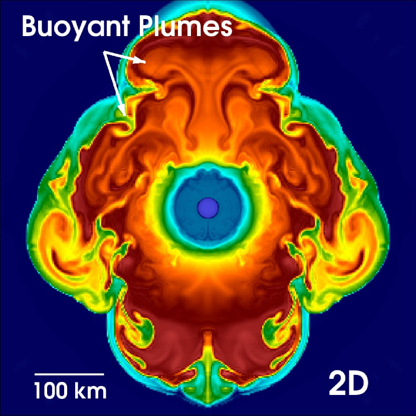
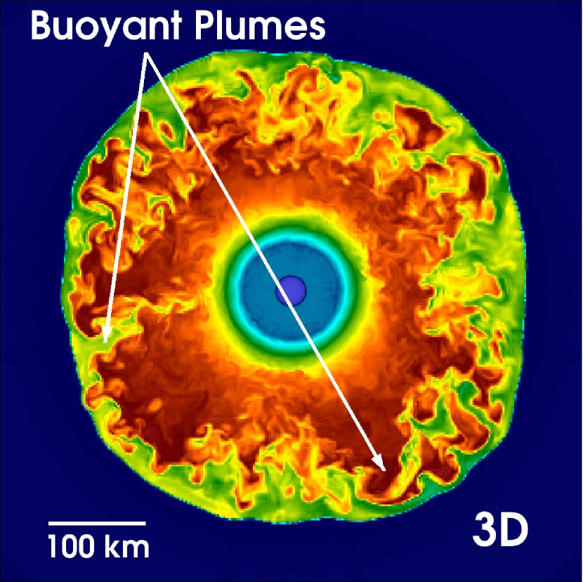
In most simulations, there are hints that buoyancy-driven convection dominates nonlinear motions. 2D and 3D simulations that include neutrinos show prominent, positively-buoyant, high-entropy plumes and negatively-buoyant, low-entropy plumes at late times (see Figure 1). Even in 2D simulations that exhibit large sloshing motions of the shock, outward excursions of the shock are accompanied by rising, high-entropy plumes. Most recently Burrows et al. (2012) and Dolence et al. (2013) have analyzed the multi-dimensional shock and turbulent motions in 2D and 3D simulations and have found that the sloshing motions frequently identified with the SASI are suppressed in 3D compared to 2D, and the character of the oscillations is sensitive to the driving neutrino luminosity. These results are consistent with neutrino-driven convection as the source for the aspherical shock motions, in that the correlation with neutrino luminosity is an obvious indicator of neutrino-driven convection. The reduction in the large-scale sloshing modes in going from 2D to 3D is consistent with known differences in turbulence between 2D and 3D (Boffetta & Ecke, 2012). In 3D, turbulence cascades to smaller scales only via a constant energy cascade. 2D turbulence exhibits a double cascade: an enstrophy cascade to smaller scales and an energy cascade to larger scales. This difference naturally leads to more large-scale, coherent structures in 2D (see Figure 1). Might this be the source for the apparent sloshing modes in realistic 2D simulations? Albeit circumstantial, these observations call into question the assumed dominance of a SASI in CCSN simulations that include neutrinos.
Determining which instability dominates, if either, requires a detailed analysis of the nonlinear motions and comparisons with theoretical predictions. Unfortunately, complete nonlinear theories do not yet exist for either a SASI mechanism or neutrino-driven convection. Therefore we can not falsify one theory or the other; Rather in this paper, we use elements of the incomplete theory and past numerical experiments to “derive” expectations for the nonlinear turbulence. The recognition of the SASI is quite recent and the body of knowledge for the nonlinear SASI is quite limited. On the other hand, the body of knowledge related to buoyancy-driven convection is older and richer. Therefore, in this paper, we focus on the latter and leave the former for future work.
To test whether the nonlinear, turbulent flows of our 3D CCSN simulations are consistent with buoyancy-driven convection, we compare these simulations with other buoyancy dominated simulations and with expected scalings of neutrino-driven convection. In Section 2, we describe the 2D and 3D simulations. Then in Section 3, we use the Reynolds-decomposed hydrodynamics equations to formulate scalings for neutrino-driven convection, and in Section 3.1, we compare these expectations with the properties of 2D and 3D simulations. Turbulence, whether it is neutrino- or SASI-driven, should expand the shock radius. While this is a trivial prediction, surprisingly, no one has verified that the shock radius is in fact larger due to this turbulence (as opposed to increased entropy in the gain region for example). In Section 4, we test whether the shock radius stalls at larger radii due to turbulence. Finally, in Section 5, we conclude that the turbulent motions in these 2D and 3D simulations are consistent with buoyancy-driven convection.
2. Simulations
The numerical results of this paper are based upon CCSN simulations using CASTRO (Almgren et al., 2010) and are similar to the simulations of Burrows et al. (2012) and Dolence et al. (2013). CASTRO solves the hydrodynamics equations using a Godunov-type finite-volume scheme where the boundary fluxes are calculated using an approximate Riemann solver (Almgren et al., 2010). Specifically, it evolves the conservative hydrodynamic equations:
| (1) |
| (2) |
and
| (3) |
where is the mass density, is the velocity, is the local gravitational acceleration, is , is the specific internal energy, is the pressure, and is the net heating and cooling. For gravity, we use the Newtonian monopole approximation, , and for pressure, we use a relativistic-mean-field equation of state (Shen et al., 1998). As initial conditions for these simulations, we use the 15- progenitor model of Woosley & Weaver (1995).111See Murphy & Burrows (2008) and Hanke et al. (2012) for representative accretion rate history curves.
Following the prescription established in Murphy & Burrows (2008) and Nordhaus et al. (2010), we approximate neutrino heating and cooling with local prescriptions, i.e.
| (4) |
where is the luminosity of electron- or anti-electron-type neutrinos in units of erg/s, is the temperature of the neutrinos (which we set to 4 MeV for all runs), is the local matter temperature, and the constants are and . For a derivation of these constants see Janka (2001). In this paper, we consider neutrino luminosity parameters of .
Absorption and emission of electron- and anti-electron-type neutrinos is most efficient on free neutrons and protons,respectively. Therefore, we weight the heating and cooling terms by the combined mass fractions of protons and neutrons, i.e. . Equation 4 is an approximation that is most relevant in the optically-thin regime. Therefore, to suppress unphysical heating and cooling at high optical depths, we further weight Equation (4) by , where is an average optical depth of the electron- and anti-electron-type neutrinos, is the neutrino opacity, and we approximate the optical depth with
| (5) |
To simulate the range in length and time scales encountered in core-collapse simulations, we use CASTRO’s adaptive-mesh-refinement (AMR) and adaptive time-stepping capabilities. We have developed an AMR strategy to simulate the full dynamic range of spherical collapse, while keeping the run-time and memory requirements as low as possible. Overall, we use six levels of refinement, each a factor of two smaller than the next largest level. The largest domain of the 3D simulations is a cube with 10,000 km on a side and has a resolution of 32 km at the coarsest level. To adequately resolve the proto-neutron star (PNS) structure, the finest level has a resolution of 0.5 km out to a radius of 50 km. In between, we initialize the refinement level () to maintain a roughly constant angular resolution of , i.e.
| (6) |
where is the floor function.
Throughout the simulation, we maintain Equation (6) as the minimum resolution. In addition, we set the minimum refinement level to 4 everywhere the entropy is greater than 5 (where is Boltzmann’s constant). Effectively, this extends level 4 refinement (2 km resolution) to include all regions interior to the stalled shock. As the shock expands during explosion, level 4 refinement expands in radius requiring ever greater memory. To limit the storage requirements of the simulation we impose maximum radii for each refinement level via
| (7) |
3. Scalings for Neutrino-Driven Convection
Comparing to a nonlinear theory for 3D neutrino-driven turbulence is the most robust way to diagnose whether turbulence is driven by buoyancy. At the moment, a complete nonlinear theory does not yet exist, but we argue that a partially complete nonlinear theory is enough to identify the driving forces of turbulence.
In particular, we use the Reynolds-decomposed hydrodynamics equations and formulate scaling relations for neutrino-driven convection. In this paper, we are not attempting to develop a complete theory for neutrino-driven convection. Developing a complete theory requires developing a 3D closure model for the Reynolds-decomposed equations. Instead, we use the Reynolds-decomposed equations to diagnose what drives turbulence. In short, the decomposed equations clearly delineate the various terms that drive, dissipate, or redistribute turbulence. We can use the results of 2D and 3D simulations to directly calculate the scale of these terms and determine which dominate. In this section, we introduce the Reynolds-decomposed equations and show how we can assess whether or not buoyancy drives convection in the 2D and 3D simulations of this paper.
The steady-state, spherically-averaged, Reynolds-decomposed conservation equations for mass, momentum, and entropy are
| (8) |
| (9) |
and
| (10) |
where is an average over solid angle and approximately one eddy turn-over time, the subscript denotes the background flow, the prime denotes the perturbation due to convection, and is the turbulent dissipation. To avoid cumbersome subscripts later, we do not use for the background velocity. Rather, the background velocity is and the perturbed velocity is , i.e. . The Reynolds-averaged equations are similar in form to the usual equations of hydrodynamics, except these equations have three new terms that are associated with turbulence. The mass equation, Equation (8), includes the divergence of the buoyancy flux, , the momentum equation includes the divergence of Reynolds stress,222For practical purposes, we calculate via , which we find to be nearly identical to . This is because when one expands into the individual terms, empirically we find that is the dominant term. Note, we could have easily defined as . However, this definition obscures the behavior of the turbulent velocities with a steep density gradient. , and the entropy equation includes the transport of entropy by the turbulent entropy flux, . For low-Mach-number flows, the buoyant flux and entropy flux can be related by a thermodynamic derivative (Murphy & Meakin, 2011), so in the rest of this paper, we consider only and .
The new turbulent terms require additional equations to close the system of equations. One should refer to Murphy & Meakin (2011) for the full set, but here we discuss only the equation for , or more specifically, we present the specific kinetic energy () equation, where is related to the trace of the Reynolds stress by . The turbulent kinetic energy equation is
| (11) |
For a spherically symmetric background flow, this equation completely describes the evolution of the turbulent kinetic energy. On the left-hand-side, we have the time rate of change of the turbulent kinetic energy, and the second term represents the redistribution of the turbulent kinetic energy by the average background flow. On the right-hand-side, we have the terms that govern the evolution: shear driving term, work done by buoyancy, turbulent redistribution by the turbulent kinetic energy flux, the divergence of the pressure flux (), work done by turbulent pressure, and turbulent dissipation.
By itself, the turbulent kinetic energy equation, Equation (11), does not completely determine the turbulent flow. For that, one must solve the full set of equations and develop a closure model for 3D à la Murphy & Meakin (2011). In the process, one must validate the full set of equations with 3D simulations, develop a 3D turbulence model for the third-order moments, and compare the 2D and 3D turbulence models. Such a task is beyond the scope of this paper. Fortunately, there is no need to develop a full turbulence model to diagnose whether the postshock turbulence is buoyancy-driven. Rather, we argue that the global properties of Equation (11) enable such a diagnosis.
Using a few standard assumptions, we now suggest a simple balance law which the 3D simulations should obey if turbulence is buoyancy driven. Assuming no shear, steady state, zero turbulent kinetic energy flux at the convective boundaries, and low Mach-number turbulent flows, we integrate Equation (11) over the entire convective volume and find a balance between global buoyant driving and global turbulent dissipation:
| (12) |
Under the aforementioned assumptions many of the terms trivially disappear, resulting in a simple balance between two terms. Note, the surface terms associated with the second term on the left-hand-side vanish not because we ignored the background flow, but because we have assumed that the turbulent kinetic energy vanishes at the convective boundaries. If the shock itself generates turbulence (as might be the case for the SASI), then this assumption may be invalid. For the moment, however, we will adopt this assumption and let comparison with 3D simulations (in Section 3.1) validate or invalidate this hypothesis.
In comparing Equation (12) with 3D simulations, calculating the integrated buoyant driving term () is straightforward. We merely use the simulations to calculate the integral, . Turbulent dissipation, , on the other hand requires a model. We adopt Kolmogorov’s hypothesis, in which the dissipation rate is set at the largest scales333Actually, the idea that dissipation starts at the largest scales and cascades to smaller scales was first proposed by Richardson (1922), but Kolmogorov (1941) established the quantitative theory that we reference in this paper. and is of order , where is a typical turbulent velocity on the largest length scale, . Upon initial inspection, it might seem that we have merely re-framed our ignorance in the parameter , and that the global balance hypothesis is not a predictive theory. However, it is indeed predictive. Global balance, Equation (12), together with Kolmogorov’s hypothesis specifically predicts that buoyant driving is proportional to the third power of the turbulent velocity, i.e.
| (13) |
This is a nontrivial, falsifiable prediction. For example, in shear-driven turbulence, rather than buoyancy, the power in shear would be proportional to the third power of the turbulent velocity. In this case, the proportionality in Equation (13) would not necessarily hold. Even if buoyancy is the dominant driving force, this proportionality may not hold. For example, may not be constant, in which case simulations would not exhibit the behavior in Equation (13). In summary, if global buoyant driving is indeed balanced by turbulent dissipation and the length scale is a constant, then we nontrivially predict the proportionality in Equation (13). In Section 3.1, we test this hypothesis with several 3D simulations spanning a wide range of driving neutrino luminosities; the simulations validate the hypothesis.
Formally, is a free parameter of the model. However, simulations of stellar models (Arnett et al., 2009) and core collapse (Murphy & Meakin, 2011) indicate that takes on the largest possible value, the radial extent of the region actively driving convection. For this paper, we find that setting to the size of the gain region satisfies global balance. In effect, is no longer a free parameter, but a condition imposed by the global structure. If the post-shock turbulence is driven by buoyancy, then the 3D simulations should be consistent with Equation (12). In Section 3.1, we show that the 3D simulations are not only consistent with the proportionality in Equation (13), but adopting the most natural length scale makes the simulations consistent with the global balance hypothesis (Equation 12).
Next, we formulate scaling relations for neutrino-driven convection. Because a detailed theory for neutrino-driven convection does not yet exist, we can not yet derive an analytic theory from first-principles. However, when a first principles derivation is out of reach, it is common practice to use dimensional analysis and experience to suggest analytic scalings and then test these with either experiment or numerics. Kolmogorov’s theory for turbulence is a classic and successful example of using this methodology. Here, we use a similar strategy to derive the scalings for neutrino-driven convection.
Our primary hypothesis is that in neutrino-driven convection, the convective power scales with the driving neutrino power (i.e. ). What are and ? Well, one might use simple dimensional analysis to guess at the form of these powers. Instead, we appeal to the governing equations to help inform an appropriate expression. Specifically, we use the integral form of the entropy equation (Equation 10). Our next major hypothesis in deriving the scalings is that the source terms in Equation (10) are of the same order. Using these terms, we suggest analytic scalings for neutrino-driven convection, and test the resulting predictions with 3D simulations in Section 3.1.
Next, we consider the entropy equation to find more appropriate expressions for and . The statement that the source terms in Equation 10 are of the same order is equivalent to
| (14) |
where . To express this in terms of , we substitute the expression for (Equation 4) into this expression, and assume that cooling is negligibly small in the heating region. Because the heating term is proportional to , Equation (14) becomes
| (15) |
where is the opacity to neutrinos. An order-of-magnitude integration of this last expression leads to
| (16) |
Therefore, if neutrino-driven convection dominates the turbulent motions, then we expect the driving neutrino power, , the maximum of the turbulent luminosity, , and the turbulent dissipation, , to be proportional to one another. For example, from these scaling relations we predict that
| (17) |
where is some constant of proportionality. Furthermore, we can now propose an expression for . Our inspection of the entropy equation suggests that and that . Note that the natural neutrino-driving power to consider is not just but , which takes into account the amount of neutrino power absorbed in the convective region. Therefore, our hypothesis becomes
| (18) |
In Section 3.1, we find that the 3D simulations are consistent with the hypotheses in Equations. (17) and (18).
3.1. Results
In this section, we present many ways in which both 2D and 3D CCSN simulations are consistent with the hypothesis that neutrino-driven convection dominates the multi-dimensional motions. Since the 3D simulations best represent Nature, we highlight the 3D results and only include the 2D results as a comparison with historical literature.
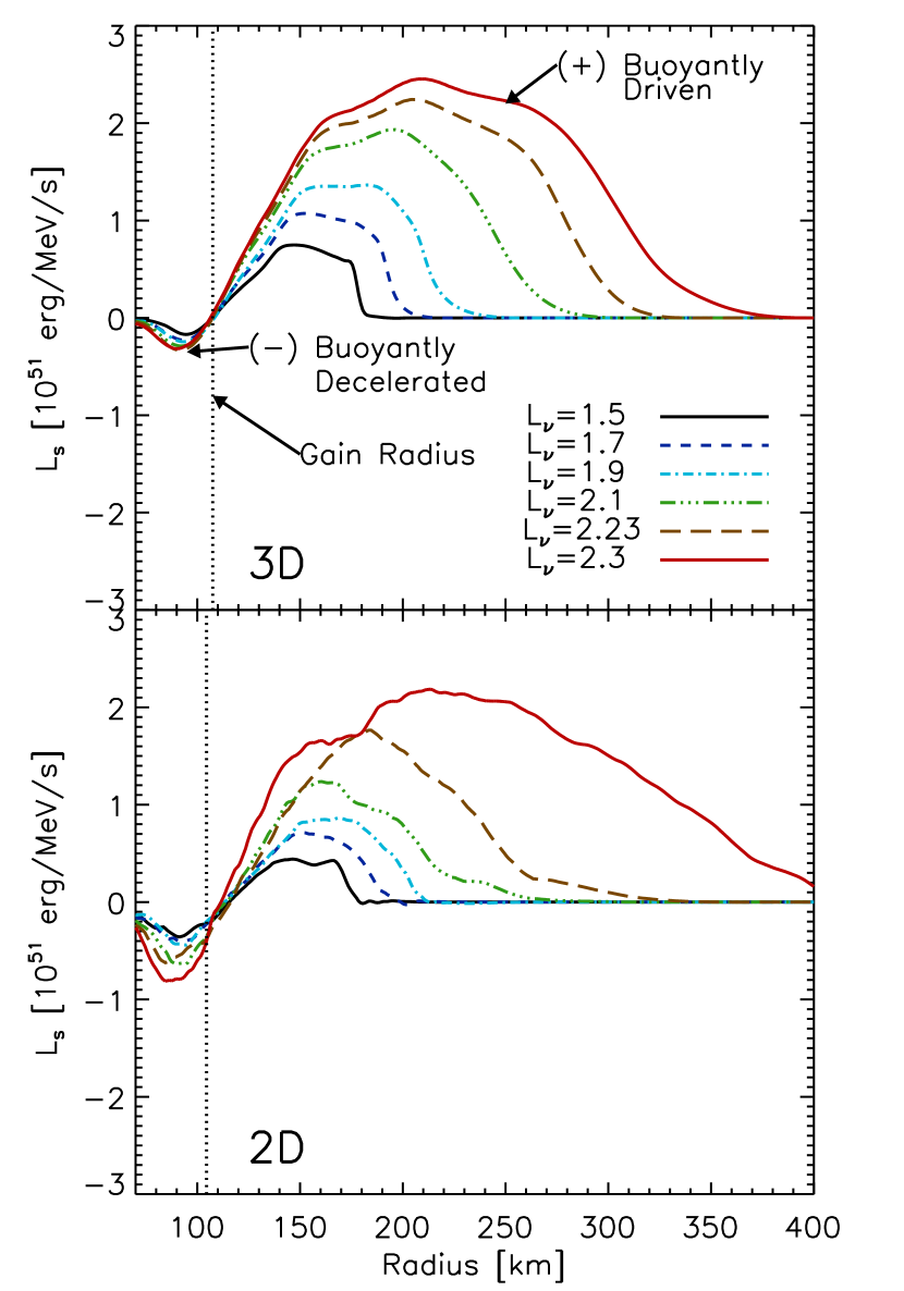
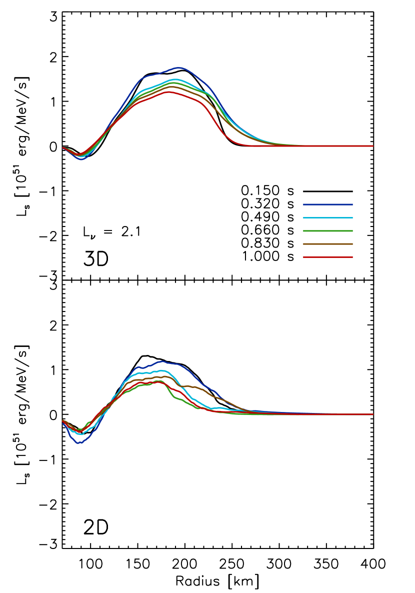
Figure 2 shows the turbulent entropy luminosity, , versus radius for six different driving neutrino luminosities at 250 ms after bounce. The gross features of these profiles are consistent with buoyancy-driven convection. In regions where buoyancy drives convection, higher entropy plumes are driven upward and lower entropy plumes sink. The net effect is that the entropy-and-velocity-perturbation correlation, (and equivalently ) is positive in the convectively active regions. As the plumes penetrate into the stable layers at the convective boundaries, the entropy perturbations flip sign. For example, sinking plumes, which had a negative entropy perturbation have, by definition, positive entropy perturbations with respect to the lower bounding layer. Hence, while is positive where buoyancy actively drives convection, is negative in the convective overshoot regions. Murphy & Meakin (2011) showed that in the gain region of 2D CCSN simulations has these characteristics, thereby suggesting that convection is buoyantly driven. Figure 2 shows that these same qualities are manifest in similar 3D CCSN simulations; once again, suggesting that turbulence in the gain region is buoyancy-driven.
Although the profiles of the 2D simulations (see also Murphy & Meakin, 2011) and the 3D simulations (this paper) are qualitatively similar, we note a few interesting and potentially important quantitative differences. Murphy & Meakin (2011) described the profile as peaking near the gain radius and sloping down linearly to either side. Specifically, they concluded that smoothly approaches zero at the shock. The 3D profiles in Figure 2 contradict this conclusion. Rather than smoothly approaching zero at the shock, is roughly constant starting at 30 km above the gain radius all the way up to the shock; at the shock, discontinuously drops to zero. We suspect that the 2D profiles actually show the same behavior as the 3D profiles and that averaging across the 2D shock causes this apparent discrepancy. Note that in the 3D profiles (Figure 2), the width of the shock smooths out the discontinuity. In the 2D simulations, the shock exhibits much larger shock oscillations (Burrows et al., 2012; Dolence et al., 2013), smoothing the discontinuity out over a much larger range of radii. Apparently, the major differences in the 2D and 3D shock morphology led to an erroneous description of the profile in Murphy & Meakin (2011). This observation deserves further confirmation (with other codes), scrutiny, and discussion, but we leave that for future work as this paper is primarily concerned with whether postshock turbulence is buoyancy driven and not the differences between 2D and 3D turbulence. As a final remark on Figure 2, the magnitude of monotonically increases with the driving neutrino luminosity. This is yet another observation that is expected for neutrino-driven convection.
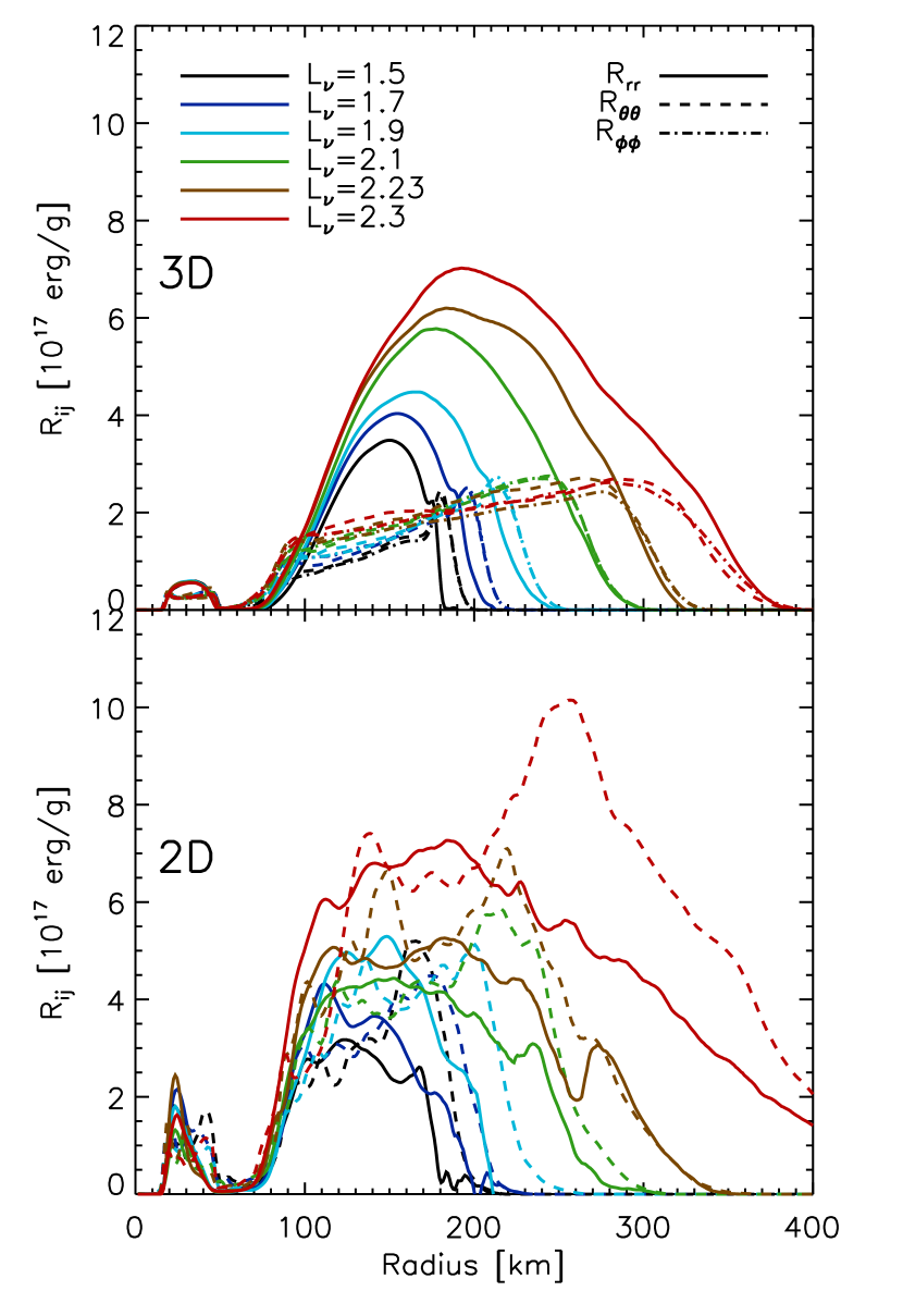
Similarly, neutrino-driven convection explains the Reynolds stresses. In Figure 3, we plot the radial (, solid line) and tangential components ( and , dashed and dot-dashed lines) of the Reynolds stress vs. radius at 250 ms after bounce for both the 2D and 3D simulations. Two characteristics of the profiles are consistent with buoyancy-driven convection. First, like , the strength of the turbulent stresses (mostly ) increases monotonically with neutrino luminosity. Secondly, the radial component of the turbulent stress is approximately equal to the combined tangential components; i.e. for 3D and for 2D. This result is consistently seen in other numerical experiments where turbulence is unambiguously driven by buoyancy (see Arnett et al. (2009), and references therein). In analytic derivations (Arnett et al., 2009; Garaud et al., 2010; Murphy & Meakin, 2011), this approximate equipartition arises because buoyancy acts first on the radial component, and then the turbulence is dissipated after energy is redistributed among the three components.
Even though the Reynolds stress profiles for both 2D an 3D are consistent with being driven by buoyancy, they are quite different in detail. For one, in the outer convective region ( km), the 3D profiles show the largest radial component at larger radii, but the 2D profiles show the largest components near the base of the convection zone. The 2D radial component is also largest at the base for the inner convective region (), but is flat in the 3D case. This implies a major qualitative difference between 2D and 3D. In 2D, the peak of at the lowest radii suggests that is dominated by the sinking plumes. Conversely, the peak of at the highest radii suggest that is dominated by the rising plumes.
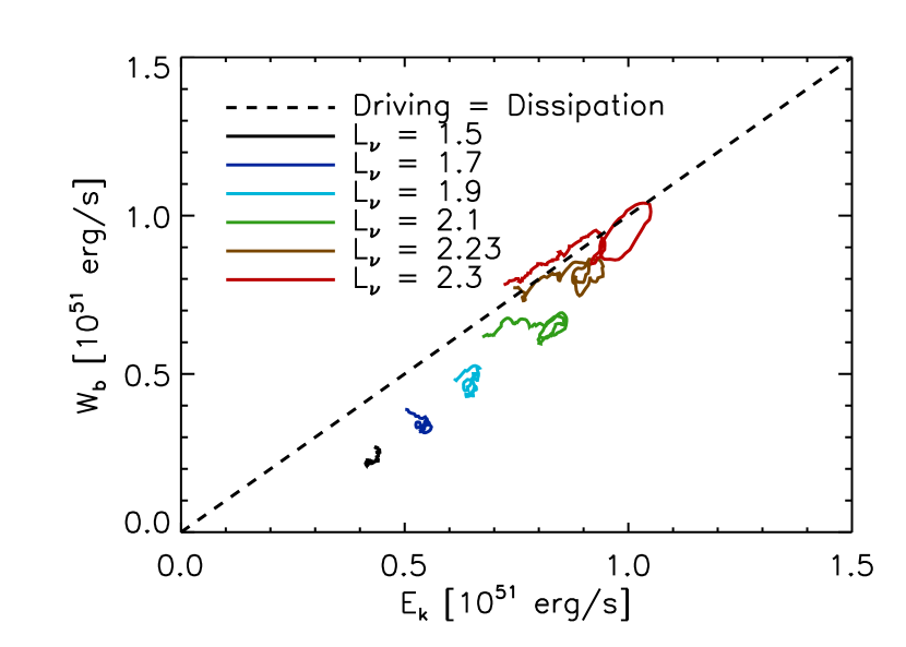
A prediction of the turbulent kinetic energy equation (Equation 11) is that globally buoyant driving is balanced by turbulent dissipation (Equation 12). This balance was also discussed in 3D stellar evolution simulations (Arnett et al., 2009) and in 2D CCSN simulations (Murphy & Meakin, 2011); here, we test whether buoyant driving is linearly proportional to the turbulent dissipation and if that constant of proportionality is of order unity. Figure 4 confirms that they are indeed proportional and the constant of proportionality is of order one. In this plot, we show global buoyant driving, , vs. global turbulent dissipation, , for several driving neutrino luminosities (delineated by color). For each luminosity, we show and for a range of times from 150 to 260 ms after bounce. The time range is chosen to be the same for all simulations, late enough to ensure a steady-state stalled shock, and early enough to avoid explosion in the highest luminosity run. As a consequence, each luminosity is not represented by a single point but a tortured line, which shows that is more or less balanced by during the entire steady-state period. In summary, Figure 4 verifies that , that the constant of proportionality is the largest scale as predicted by Kolmogorov, and that global buoyant driving roughly balances global turbulent dissipation.
Though buoyant driving is proportional to , it does not exactly equal it. At the highest luminosity, near explosion they are nearly equal, but at the lowest luminosity, is roughly half of . There are several possible reasons for this lack of exact equality. First, the definition of is suggested by dimensional analysis and is not an exact derivation. For example, even though the size of the gain region may be a good estimate for at the highest luminosities, it may not be at the smallest luminosities. Second, in deriving Equation (12), we assumed for simplicity that the turbulent kinetic energy fluxes at the shock are zero. The fluxes may not be exactly zero444As might be the case for the SASI., but small for large luminosities and relatively large for small luminosities. In either scenario, the fact that and are proportional and are of the same order suggests that turbulent dissipation is mostly balanced by buoyant driving, and whatever is missing is a slight correction to this basic conclusion at the lowest luminosities. This might be an indication of substantial SASI motions at the lowest luminosities (Burrows et al., 2012; Dolence et al., 2013).
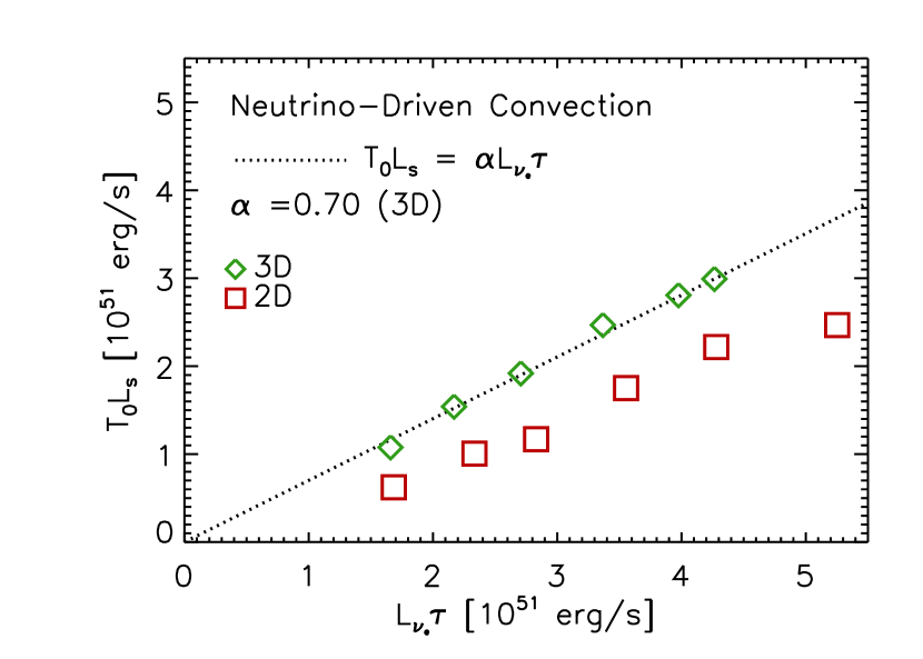
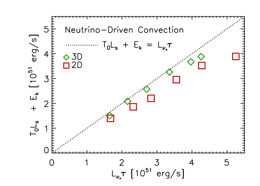
In Section 3, we argue that the convective luminosity, , and turbulent dissipation, , are each proportional to the driving neutrino-power, . Furthermore, we propose that the driving neutrino power is distributed between the convective powers, i.e. . Figures 5 and 6 compare these analytic scalings, Equations (17 and 18), (dotted lines) with the results from the 2D (squares) and 3D (diamonds) simulations. Indeed, the turbulent luminosity (Figure 5) is linearly proportional to the driving neutrino power for both 2D and 3D. Interestingly, the constant is lower for the 2D simulations, suggesting that 2D is less efficient at driving a convective entropy luminosity than 3D. To calculate the constant of proportionality for 3D, we merely report the ratio of the luminosities at the last 3D point. In Figure 6, we find that the 2D and 3D simulations confirm the hypothesis of Equation (18) that the neutrino-driving power is distributed among the convective powers. In summary, our simulations confirm our predictions that turbulence scales with neutrino power, as is expected in buoyant convection. A result we could not predict, but that the simulations tell us, is that convection is more vigorous for 3D than 2D for the same luminosity. In the Appendix, we show that the scalings persist throughout the steady-state accretion phase.
4. Expansion of Shock Radius due to Turbulence
An important aspect of the core-collapse problem is the presence of the standing accretion shock, so we also consider how turbulence affects the stalled shock radius. Formally, the stalled shock is located where the upstream and the downstream profiles satisfy the Rankin-Hugoniot jump conditions. For zero shock velocity, the mass flux, momentum flux, and energy flux conditions are
| (19) |
| (20) |
and
| (21) |
In detail, the shock position is a nontrivial solution to a boundary value problem for , , and . However, with a few reasonable approximations, the shock boundary condition can be reduced to one expression. First, we assume steady-state and that the mass accretion rate () is constant. Second, we assume that the upstream flow is in near free-fall and essentially pressureless. Third, we assume for the purposes of this argument that the equation of state is approximated by a -law, i.e. . The first and second assumptions completely determine the upstream flow as a function of radius. Because the upstream flow is pressureless, we use the strong shock limit to determine the shock compression ratio, i.e. . Under these assumptions, the full Rankine-Hugoniot jump conditions reduce to a single expression:
| (22) |
where () denotes upstream (downstream) state variables. Since the term in parentheses is 1, the shock conditions reduce to an expression that demands a balance between the upstream ram pressure and the downstream thermal pressure. In essence, one can use the momentum jump condition (Equation 20) to illuminate the balancing conditions at the shock. From here on, we focus on the momentum jump condition with zero pressure on the upstream side, i.e.
| (23) |
Using Reynolds decomposition, the momentum jump condition becomes
| (24) |
where the velocities, and , are background velocities. Hence, the new shock position is located where the post-shock thermal, ram, and turbulent ram pressures balance the pre-shock ram pressure. The addition of the turbulent ram pressure may result in larger shock radii.
Equation (24) by itself is not enough to determine the shock position. One must also specify the pre-shock and post-shock profiles, and it is the intersection of these profiles that determines the shock radius. The pre-shock ram pressure is given by free-fall assumptions, resulting in a fixed, relatively shallow profile (e.g. ). The post-shock region is in sonic contact and in rough hydrostatic equilibrium, so the postshock pressure depends upon physics (such as cooling) of the entire postshock region. Fortunately, though, the post-shock pressure profile can be expressed by a simple power-law (e.g. ), where the normalization depends upon the details of cooling, etc.; we fit power-laws to the pre-shock and post-shock profiles of 3D simulations and use Equation (24) to predict the average shock radius with and without turbulent ram pressure. We calculate the correct average shock radius only if we include the turbulent ram pressure.
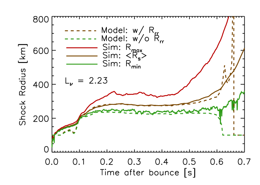
Figures 7 and 8 show that turbulent ram pressure explains in part the expansion of the shock radius. Figure 7 shows for one representative neutrino luminosity fits to the upstream ram pressure (dotted line) and downstream thermal, ram, and turbulent pressures (solid line), as a function of radius. Using these pressure profiles, we calculate the shock to be located where the upstream and downstream fits cross. For comparison we show the actual solid-angle-averaged shock radius () from a 3D simulation (dot-dot-dot-dashed line). Including the turbulent pressure leads to a more accurate prediction of the shock radius. If we neglect the turbulent pressure, then we estimate a shock radius that is smaller by about 40 km (labeled “ w/o ”). To be clear, we are not concluding that this is where the shock would be located in the absence of turbulent pressure (i.e. a 1D simulation, although it is quite close). We are merely demonstrating that the turbulent ram pressure is a sizable fraction of the microscopic pressure and that one can not ignore the importance of the turbulent pressure.

Figure 8 shows the resulting shock locations as a function of driving neutrino luminosity. This plot shows the modeled shock radii, including turbulent ram pressure (solid line) and the modeled shock radii excluding turbulent ram pressure (dashed line). For comparison, we show the calculated minimum (triangles), average (diamonds), and maximum (squares) shock radii for 3D simulations, all at 250 ms after bounce555In the Appendix, we plot these results at other times after bounce and find that our results and conclusions hold throughout the steady state accretion phase.. Including turbulent pressure in the post-shock profile predicts shock radii that agree with the measured average shock radius. Excluding the turbulent pressure under-predicts the average shock radius. On the other hand, excluding the turbulent pressure gives shock radius predictions that are consistent with the minimum shock radii. This suggests that the minimum shock radii occur at places and times where the fluctuating turbulent motions are instantaneously negligible. On average though, the turbulent motions are not negligible and influence the average shock radius.

Showing that turbulent ram pressure causes expansion of the shock radius does not by itself prove that buoyant-driven convection is responsible for the expansion. Any instability that leads to turbulence would give a similar prediction. However, the dependency of the shock radii and the turbulent pressure on does strongly suggest the prominence of neutrino-driven convection.
5. Conclusions and Discussion
We have identified in Section 3 four ways in which the aspherical, nonlinear flow of 3D CCSN simulations is consistent with buoyancy-driven convection. First, the turbulent luminosity is positive in the gain region where buoyancy actively drives convection, and the turbulent luminosity is negative in the stably-stratified region where buoyancy decelerates convective plumes. Second, the radial component of the Reynolds stress is in rough equipartition with the tangential components, i.e. ; this result is observed in other contexts of buoyancy-driven convection and is expected when convection is driven radially, but dissipated among all the components (Arnett et al., 2009; Garaud et al., 2010; Murphy & Meakin, 2011). Third, we find that turbulent dissipation is balanced by buoyant driving. Fourth, both the turbulent luminosity and turbulent dissipation scale with the driving neutrino power. In essence, these results are consistent with the hypothesis that neutrino-driven convection is the dominant multi-dimensional instability in our 3D CCSN simulations.
Since these results are consistent with the buoyancy-driven hypothesis, one wonders if the SASI is suppressed during neutrino-driven explosions. Of course, our results do not prove that the SASI is absent. Rather, they suggest that the nonlinear motions are merely consistent with buoyant convection and that if the SASI is present it mimics buoyant convection, or is subdominant. Numerous analytic and numerical studies have shown that if the conditions are right, a nonlinear SASI arises. However, these studies were performed largely in the absence of neutrino heating or used high accretion rates and small initial perturbations. A few did include neutrinos, and given sufficient initial perturbations, even in these investigations neutrino-driven convection seems eventually to dominate (Foglizzo et al., 2006; Scheck et al., 2008; Fernández & Thompson, 2009; Müller et al., 2012; Hanke et al., 2013). It appears that in attempting to isolate the SASI mechanism, researchers were suppressing the dominant nonlinear instability in core-collapse simulations.
Minimally, there are two hypotheses for the dominant multi-dimensional instability: the SASI and buoyancy-driven convection. Our results suggest that when neutrinos drive explosions, they also drive convection and turbulence. However, there is as yet no self-consistent theory for a nonlinear SASI mechanism, so we cannot test the SASI at this time. In fact, it is entirely possible that convective and SASI theories might predict similar characteristics. For example, in both cases, turbulence is most likely dissipated in accord with Kolmogorov’s hypothesis. However, we have shown that turbulent dissipation is balanced by buoyant driving, which seems an unlikely prediction of a nonlinear SASI theory. In any case, it is clear that a nonlinear theory for the SASI must be developed before we can definitively claim that the SASI is subdominant. Furthermore, even though our approximations are designed to closely mimic more self-consistent simulations, a robust conclusion on the importance of convection must wait for full 3D neutrino-transport hydrodynamic simulations.
In the meantime, we have shown that the turbulence in our 3D simulations is consistent with buoyant convection. Not surprisingly, we find that neutrino-driven convection accompanies neutrino-driven explosions.
Acknowledgments
The authors acknowledge stimulating interactions with Jason Nordhaus, Ann Almgren, and Thomas Janka. A.B. is supported by the Scientific Discovery through Advanced Computing (SciDAC) program of the DOE, under grant number DE-FG02-08ER41544, the NSF under the subaward no. ND201387 to the Joint Institute for Nuclear Astrophysics (JINA, NSF PHY-0822648), and the NSF PetaApps program, under award OCI-0905046 via a subaward no. 44592 from Louisiana State University to Princeton University. The authors would like to thank the members of the Center for Computational Sciences and Engineering (CCSE) at LBNL for their invaluable support for CASTRO. The authors employed computational resources provided by the TIGRESS high performance computer center at Princeton University, which is jointly supported by the Princeton Institute for Computational Science and Engineering (PICSciE) and the Princeton University Office of Information Technology; by the National Energy Research Scientific Computing Center (NERSC), which is supported by the Office of Science of the US Department of Energy under contract DE-AC03-76SF00098; and on the Kraken supercomputer, hosted at NICS and provided by the National Science Foundation through the TeraGrid Advanced Support Program under grant number TG-AST100001.
In this paper, we address which mechanism drives turbulence during the stalled accretion phase and thereby sets the stage for explosion. In this appendix, we consider the validity of our conclusions as a function of time. We find that the temporal behavior falls into two distinct classes: those that explode within 1 s after bounce and those that don not. Rather than showing the time evolution for all neutrino luminosities, we present only two neutrino luminosities; one represents a non-exploding model (), and one represents an exploding model (). As is expected, we find that our conclusions are valid during the steady-state accretion phases and are less valid during the dynamic phases, which include the initial phase when the shock is settling and the explosive phase.
Figures 9-12 show the temporal evolution of the turbulent entropy luminosity and the Reynolds’ stress for the 2D and 3D simulations. During the steady-state accretion phase, both measures of turbulence are consistent with buoyant driven convection. The turbulent entropy luminosity is positive where buoyancy actively drives turbulence and negative where the stable layer decelerates the convective plumes. Furthermore, the distribution of Reynolds’ stresses is roughly in equipartition between the radial and tangential components and is a hallmark of buoyancy driving in the radial direction. For both the non-exploding and exploding model, the convective velocities as measured by the Reynolds’ stress increases with time, especially during the steady-state accretion phase. However, the convective entropy luminosity decreases with time for the non-exploding model and is non-monotonic for the exploding model.
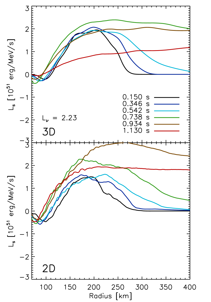
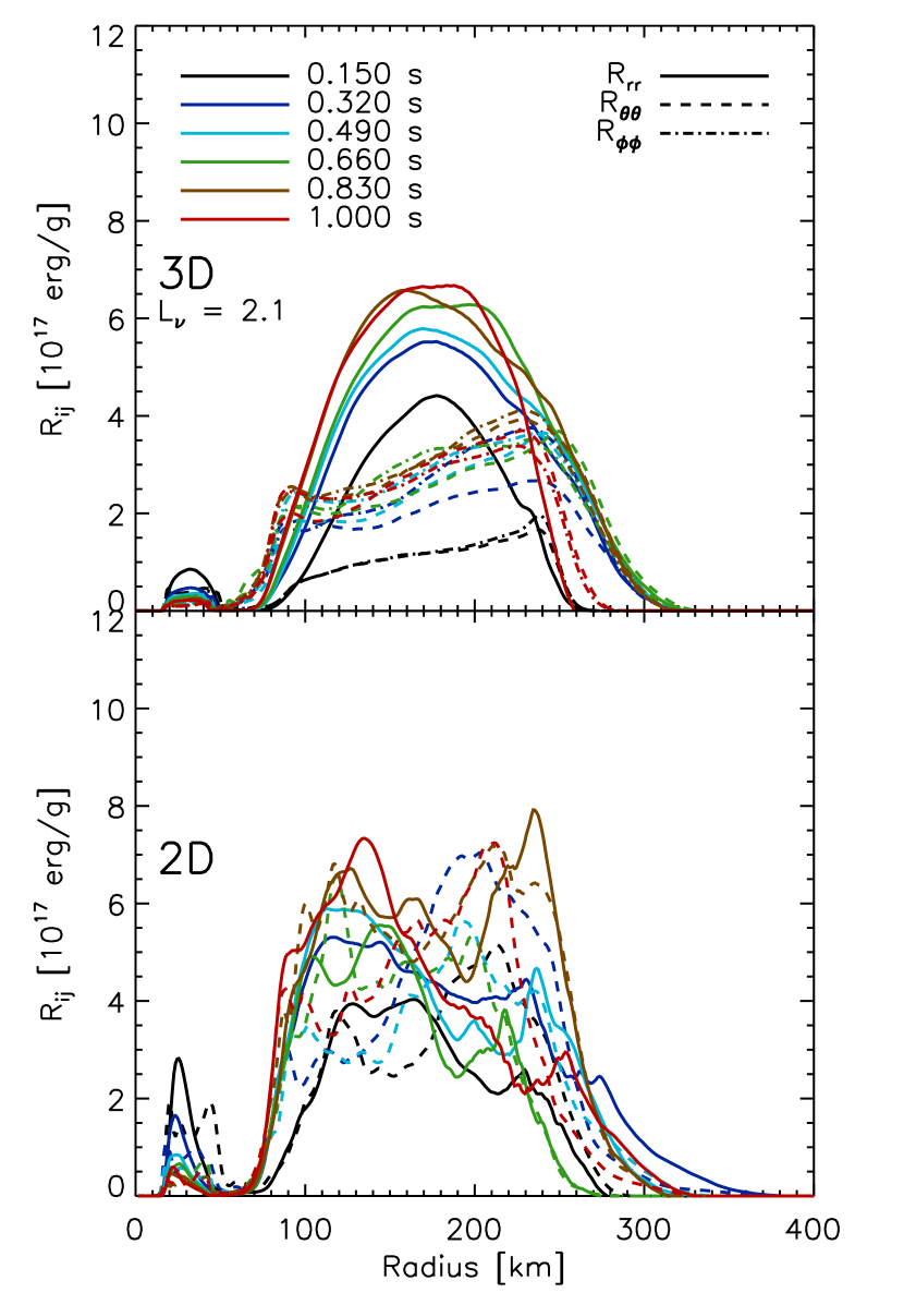
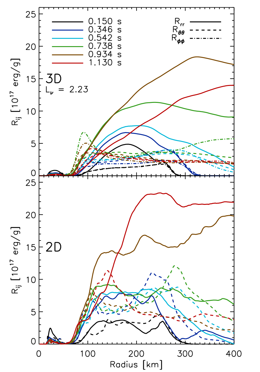
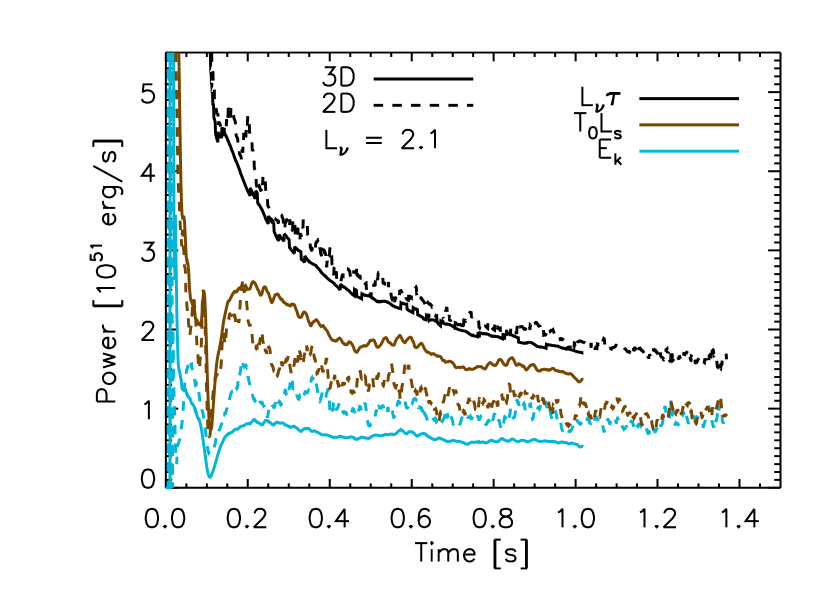
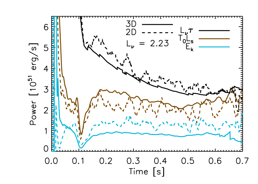
In Figures 13-16, we demonstrate that the convetive power scales with the driving neutrino power, , throughout the steady-state accretion phase. First, we plot in Figures 13 & 14 the driving neutrino power (), the convective luminosity (), and the turbulent dissipation rate () versus time after bounce. We show both 2D and 3D results for the non-exploding (, Figure 13) and exploding (, Figure 14) models. Comparing these measures of power is most meaningful during the steady-state accretion phase: later than 0.15 s and earlier than explosion. The does not explode during the calculation, so we consider the full run. The model, on the other hand, explodes at 0.6 s after bounce. Therefore, we do not plot the powers beyond 0.65 s. Beyond this time, these powers, especially , are ill defined, difficult to calculate, and confusing to interpret. Finally, in Figures 15 and 16, we plot the ratio of convective power to driving neutrino power, which we expect to be of order one.
In general, Figures 13-16 show that the scaling relations presented in this paper persist during the steady accretion rate phase. Figures 13 and 14 show that the turbulent dissipation is higher for 2D than 3D, but that the turbulent entropy luminosity is higher for 3D than 2D. The first result is a consequence of the fact that the radial convective velocities are higher in 2D than 3D. Given the lower convective velocities in 3D, the material can dwell longer in the gain region; this is possibly the explanation for the larger convective entropy luminosity. The most striking result of Figures 13-16 is that despite the fact that the driving neutrino power varies by a large factor (4 for ), the ratio remains of order one during the entire steady-state accretion phase. In other words, the scaling relation between the driving power and the convective powers persists.


Finally, Figure 17 shows that our model for calculating the shock radii (with and without turbulent pressure) is valid for the entire steady-state accretion phase.
References
- Almgren et al. (2010) Almgren, A. S., Beckner, V. E., Bell, J. B., Day, M. S., Howell, L. H., Joggerst, C. C., Lijewski, M. J., Nonaka, A., Singer, M., & Zingale, M. 2010, ApJ, 715, 1221
- Arnett et al. (2009) Arnett, D., Meakin, C., & Young, P. A. 2009, ApJ, 690, 1715
- Bazan & Arnett (1998) Bazan, G., & Arnett, D. 1998, ApJ, 496, 316
- Benz et al. (1994) Benz, W., Colgate, S. A., & Herant, M. 1994, Physica D Nonlinear Phenomena, 77, 305
- Bethe (1990) Bethe, H. A. 1990, Reviews of Modern Physics, 62, 801
- Bethe & Wilson (1985) Bethe, H. A., & Wilson, J. R. 1985, ApJ, 295, 14
- Blondin & Mezzacappa (2006) Blondin, J. M., & Mezzacappa, A. 2006, ApJ, 642, 401
- Blondin et al. (2003) Blondin, J. M., Mezzacappa, A., & DeMarino, C. 2003, ApJ, 584, 971
- Boffetta & Ecke (2012) Boffetta, G., & Ecke, R. E. 2012, Annu. Rev. Fluid Mech., 427
- Bruenn et al. (2013) Bruenn, S. W., Mezzacappa, A., Hix, W. R., Lentz, E. J., Bronson Messer, O. E., Lingerfelt, E. J., Blondin, J. M., Endeve, E., Marronetti, P., & Yakunin, K. N. 2013, ApJ, 767, L6
- Buras et al. (2003) Buras, R., Rampp, M., Janka, H.-T., & Kifonidis, K. 2003, Physical Review Letters, 90, 241101
- Burrows (1987) Burrows, A. 1987, ApJ, 318, L57
- Burrows et al. (2007) Burrows, A., Dessart, L., & Livne, E. 2007, in American Institute of Physics Conference Series, Vol. 937, Supernova 1987A: 20 Years After: Supernovae and Gamma-Ray Bursters, ed. S. Immler & R. McCray, 370–380
- Burrows et al. (2012) Burrows, A., Dolence, J. C., & Murphy, J. W. 2012, ApJ, 759, 5
- Burrows et al. (1995) Burrows, A., Hayes, J., & Fryxell, B. A. 1995, ApJ, 450, 830
- Dolence et al. (2013) Dolence, J. C., Burrows, A., Murphy, J. W., & Nordhaus, J. 2013, ApJ, 765, 110
- Epstein (1979) Epstein, R. I. 1979, MNRAS, 188, 305
- Fernández (2010) Fernández, R. 2010, ApJ, 725, 1563
- Fernández & Thompson (2009) Fernández, R., & Thompson, C. 2009, ApJ, 703, 1464
- Foglizzo (2009) Foglizzo, T. 2009, ApJ, 694, 820
- Foglizzo et al. (2012) Foglizzo, T., Masset, F., Guilet, J., & Durand, G. 2012, Physical Review Letters, 108, 051103
- Foglizzo et al. (2006) Foglizzo, T., Scheck, L., & Janka, H.-T. 2006, ApJ, 652, 1436
- Garaud et al. (2010) Garaud, P., Ogilvie, G. I., Miller, N., & Stellmach, S. 2010, MNRAS, 407, 2451
- Guilet & Foglizzo (2012) Guilet, J., & Foglizzo, T. 2012, MNRAS, 421, 546
- Hanke et al. (2012) Hanke, F., Marek, A., Müller, B., & Janka, H.-T. 2012, ApJ, 755, 138
- Hanke et al. (2013) Hanke, F., Mueller, B., Wongwathanarat, A., Marek, A., & Janka, H.-T. 2013, ArXiv e-prints
- Herant et al. (1992) Herant, M., Benz, W., & Colgate, S. 1992, ApJ, 395, 642
- Herant et al. (1994) Herant, M., Benz, W., Hix, W. R., Fryer, C. L., & Colgate, S. A. 1994, ApJ, 435, 339
- Iwakami et al. (2008) Iwakami, W., Kotake, K., Ohnishi, N., Yamada, S., & Sawada, K. 2008, ApJ, 678, 1207
- Janka (2001) Janka, H.-T. 2001, A&A, 368, 527
- Janka & Müller (1995) Janka, H.-T., & Müller, E. 1995, ApJ, 448, L109
- Janka & Müller (1996) —. 1996, A&A, 306, 167
- Kitaura et al. (2006) Kitaura, F. S., Janka, H.-T., & Hillebrandt, W. 2006, A&A, 450, 345
- Kolmogorov (1941) Kolmogorov, A. N. 1941, Dokl. Akad. Nauk SSSR, 299
- Kuroda et al. (2012) Kuroda, T., Kotake, K., & Takiwaki, T. 2012, ApJ, 755, 11
- Lentz et al. (2012) Lentz, E. J., Mezzacappa, A., Bronson Messer, O. E., Hix, W. R., & Bruenn, S. W. 2012, ApJ, 760, 94
- Liebendörfer et al. (2001a) Liebendörfer, M., Mezzacappa, A., & Thielemann, F.-K. 2001a, Phys. Rev. D, 63, 104003
- Liebendörfer et al. (2001b) Liebendörfer, M., Mezzacappa, A., Thielemann, F.-K., Messer, O. E., Hix, W. R., & Bruenn, S. W. 2001b, Phys. Rev. D, 63, 103004
- Liebendörfer et al. (2005) Liebendörfer, M., Rampp, M., Janka, H.-T., & Mezzacappa, A. 2005, ApJ, 620, 840
- Marek & Janka (2009) Marek, A., & Janka, H.-T. 2009, ApJ, 694, 664
- Meakin & Arnett (2007) Meakin, C. A., & Arnett, D. 2007, ApJ, 665, 690
- Müller et al. (2012) Müller, B., Janka, H.-T., & Heger, A. 2012, ApJ, 761, 72
- Murphy & Burrows (2008) Murphy, J. W., & Burrows, A. 2008, ApJ, 688, 1159
- Murphy & Meakin (2011) Murphy, J. W., & Meakin, C. 2011, ApJ, 742, 74
- Nordhaus et al. (2010) Nordhaus, J., Burrows, A., Almgren, A., & Bell, J. 2010, ApJ, 720, 694
- Ohnishi et al. (2006) Ohnishi, N., Kotake, K., & Yamada, S. 2006, ApJ, 641, 1018
- Ott et al. (2013) Ott, C. D., Abdikamalov, E., Mösta, P., Haas, R., Drasco, S., O’Connor, E. P., Reisswig, C., Meakin, C. A., & Schnetter, E. 2013, ApJ, 768, 115
- Rampp & Janka (2002) Rampp, M., & Janka, H.-T. 2002, A&A, 396, 361
- Richardson (1922) Richardson, L. F. 1922, Weather Prediction by Numerical Process (Cambridge: Cambridge University Press)
- Sato et al. (2009) Sato, J., Foglizzo, T., & Fromang, S. 2009, ApJ, 694, 833
- Scheck et al. (2008) Scheck, L., Janka, H.-T., Foglizzo, T., & Kifonidis, K. 2008, A&A, 477, 931
- Shen et al. (1998) Shen, H., Toki, H., Oyamatsu, K., & Sumiyoshi, K. 1998, Nuclear Physics A, 637, 435
- Sumiyoshi et al. (2005) Sumiyoshi, K., Yamada, S., Suzuki, H., Shen, H., Chiba, S., & Toki, H. 2005, ApJ, 629, 922
- Takiwaki et al. (2012) Takiwaki, T., Kotake, K., & Suwa, Y. 2012, ApJ, 749, 98
- Thompson et al. (2003) Thompson, T. A., Burrows, A., & Pinto, P. A. 2003, ApJ, 592, 434
- Wilson & Mayle (1988) Wilson, J. R., & Mayle, R. W. 1988, Phys. Rep., 163, 63
- Woosley & Weaver (1995) Woosley, S. E., & Weaver, T. A. 1995, ApJS, 101, 181
- Yamasaki & Yamada (2006) Yamasaki, T., & Yamada, S. 2006, ApJ, 650, 291