Using data as a probe of the concordance model
Abstract
Direct observations of the Hubble rate, from cosmic chronometers and the radial baryon acoustic oscillation scale, can out-perform supernovae observations in understanding the expansion history, because supernovae observations need to be differentiated to extract . We use existing data and smooth the data using a new Gaussian Processes package, GaPP, from which we can also estimate derivatives. The obtained Hubble rate and its derivatives are used to reconstruct the equation of state of dark energy and to perform consistency tests of the CDM model, some of which are newly devised here. Current data are consistent with the concordance model, but are rather sparse. Future observations will provide a dramatic improvement in our ability to constrain or refute the concordance model of cosmology. We produce simulated data to illustrate how effective data will be in combination with Gaussian Processes.
I Introduction
Different methods and data sets are being used to reconstruct the dark energy (DE) equation of state and thereby also to test the concordance model (which has ). The results vary significantly according to the methods and data sets used, and the error bars and uncertainties are large. It is clear that higher-precision data are needed for an effective reconstruction and for robust testing of models. But just as important, more effort is needed to improve the statistical methods and the design of observational tests. In particular, there is a need for effective model-independent statistical methods and for tests that target the concordance model.
One of the most direct ways to reconstruct is via supernovae (SNIa) observations that give the luminosity distance . Model-independent approaches to reconstructing have been developed weller_albrecht ; Alam:2003sc ; daly ; Alam:2004jy ; Wang:2004py ; Daly:2004gf ; Sahni:2006pa ; Shafieloo:2005nd ; Zunckel:2007jm ; EspanaBonet:2008zz ; Genovese:2008sw ; Bogdanos:2009ib ; Clarkson:2010bm ; Holsclaw:2010sk ; Crittenden:2011aa ; Shafieloo:2012yh ; Lazkoz:2012eh ; Shafieloo:2012ht ; Seikel . SNIa observations lead indirectly to via the derivative . Then we need the second derivative of to reconstruct . This is very challenging for any reconstruction technique since any noise on the measured will be magnified in the derivatives. The problem can be lessened if direct data are used because only the first derivative needs to be calculated to determine .
In this paper we focus on observations that directly give . Presently, this may be derived from differential ages of galaxies (‘cosmic chronometers’) and from the radial baryon acoustic oscillation (BAO) scale in the galaxy distribution. Compared to SNIa observations, less observational data are needed to reconstruct with the same accuracy. For the cosmic chronometer data, it has been estimated Ma:2010mr that 64 data points with the accuracy of the measurements in Stern are needed to achieve the same reconstruction accuracy as from the Constitution SNIa data Hicken .
We use a model-independent method for smoothing data to also perform consistency tests of the concordance model (flat CDM) and of curved CDM models. These consistency tests are formulated as functions of and its derivatives which are constant or zero in CDM, independently of the parameters of the model (see Clarkson (2012) for a review). Deviations from a constant function indicate problems with our assumptions about dark energy, theory of gravity, or perhaps something else, but without the usual problems of postulating an alternative to CDM. Some of the tests we use here are given for the first time.
Gaussian processes (GP) provide a model-independent smoothing technique that can meet the challenges of reconstructing derivatives from data Rasmussen ; MacKay . We follow the same GP approach that has been applied to supernova data in a previous work Seikel by some of the authors of this paper. We use GaPP (Gaussian Processes in Python), their publicly available code111http://www.acgc.uct.ac.za/~seikel/GAPP/index.html. (See Holsclaw:2010sk ; Shafieloo:2012ht for different uses of GP in this context.) A brief description of the GP algorithm is given in Appendix A.
II Testing CDM
The Friedmann equation,
| (1) | |||||
can be rearranged to give
| (2) |
In principle, given data we can smooth it, attempt to estimate its derivative, and reconstruct . However, reconstruction of is compromised by various difficulties. It depends on the values of and , so we need independent information about these parameters when we reconstruct from data. These are difficult to estimate without assuming a form for Clarkson:2007bc ; Hlozek:2008mt ; Kunz:2012aw .
These difficulties reflect the fact that we cannot use data to construct physical models – rather, we need to use data to test physical models. The CDM model could be tested by looking for deviations from . However, there is a more focused approach: to develop null hypotheses for CDM, independently of the parameters and Clarkson (2012).
To test the concordance model – i.e. flat CDM – we can use (1) to define a diagnostic function of redshift Sahni:2008xx ; Zunckel:2008ti ; Shafieloo:2009hi :
| (3) |
Then
If is not a constant, this is a signal of an alternative dark energy or modified gravity model. Given observed data, we can estimate confidence limits for . If these are not consistent with a constant value, we can rule out the concordance model.
It is more effective to measure deviations from zero than from a constant. The more effective diagnostic is thus the vanishing of the derivative . This is equivalent to , where Zunckel:2008ti
| (4) |
The null test is therefore
To apply this test, we need to reconstruct from the data.
If the concordance model is ruled out, it is still possible that a curved CDM model describes the Universe. Equations (1) and (2) (with ) form a linear system for and . Solving for these parameters we can define
| (5) | |||||
| (6) |
and we have
These quantities are equivalent to those derived in Clarkson:2009jq in terms of , the dimensionless comoving luminosity distance. The forms contain second derivatives whereas the forms above contain only first derivatives . Given observed Hubble rate data from which we can estimate the derivative , we can then estimate confidence limits for and . If these are not consistent with a constant value, we can rule out CDM in general, and conclude that dark energy has (or there is modified gravity).
The more effective diagnostic of these consistency tests is the vanishing of the derivatives of (5) and (6). The vanishing of is equivalent to , where
| (7) | |||||
Then
The vanishing of does not give any independent information – it is also equivalent to .
Given observations of , we can construct this function independently of the parameters of the model and test CDM by measuring consistency with zero. This has the advantage that it is easier to detect deviations from zero rather than a constant, but at the expense of requiring an extra derivative in the observable. This is akin to detecting deviations from constant in , but without reliance on the parameters of the model.
For the application of these consistency tests, it is crucial to use a model-independent method to reconstruct , , , and . Model-dependent approaches have the problem that they affect or even determine the outcome of the consistency test: While fitting a CDM model to the data would always lead to a result that is consistent with CDM, fitting a model that does not include CDM as a special case would result in inconsistencies with CDM. The only model-dependent approches that do not entirely determine the outcome of the test are those assuming a model which includes CDM as a special case. Nevertheless, they affect the result by forcing the data into a specific parametrisation, which might not reflect the true model. The only way to avoid this problem is to use a non-parametric approach. Here, we use Gaussian processes, which are described in Appendix A.
III Reconstruction and consistency tests from data
Cosmic chronometers are based on observations of the differential ages of galaxies Stern ; Jimenez:2001gg ; Crawford:2010rg ; Moresco:2012jh . The Hubble rate at an emitter with redshift is
| (8) |
where is the proper time of emission. The differential method uses passively evolving galaxies formed at the same time to determine the age difference in a small redshift bin , assuming a Friedmann background. To find old galaxies sharing the same formation time, we have to look for the oldest stars in both galaxies and show that they have the same age. This method is effective; but while the differential approach significantly reduces the systematics that would be present when determining the absolute ages of galaxies, it still faces uncertainties due to the assumptions that are made to estimate the age.
The second way to measure is the observed line-of-sight redshift separation of the baryonic acoustic oscillation (BAO) feature in the galaxy 2-point correlation function Gaztanaga:2008xz ; Chuang ; Blake:2012pj ,
| (9) |
where is the sound horizon at the baryon drag epoch.
Results: real data
We use the following data sets:
CC: 18 cosmic chronometer data points Moresco:2012by .
BAO: 6 radial BAO data points Blake:2012pj ; Gaztanaga:2008xz ; Chuang .
CC+BAO: Combination of CC and BAO sets.
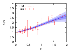
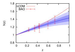
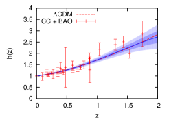
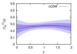
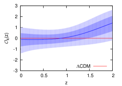
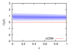
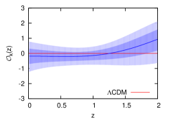
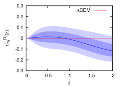
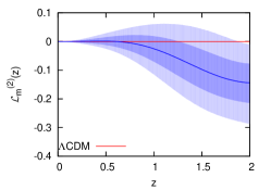
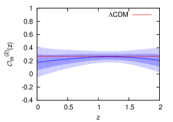
We normalize using km s-1Mpc-1. The uncertainty in is transferred to as The reconstructed functions and are shown in Fig. 1. The shaded regions correspond to the 68% and 95% confidence levels (CL). The true model is expected to lie 68% of the plotted redshift range within the 68% CL. Note that this is only an expectation value. The actual value for a specific function may deviate from the expectation. The dependence of the actual percentage on the smoothness of the function has been analysed in Seikel .
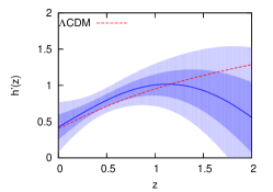
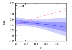
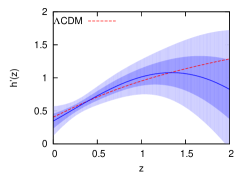
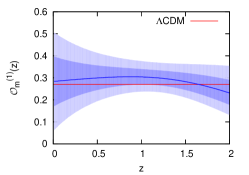
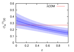
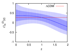
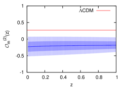
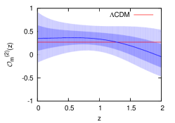
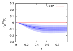
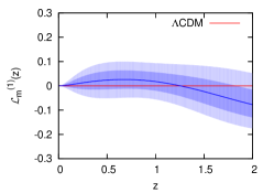
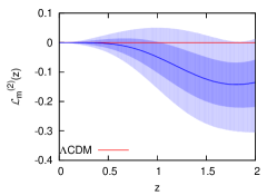
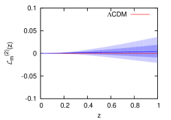
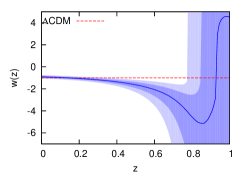
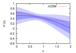
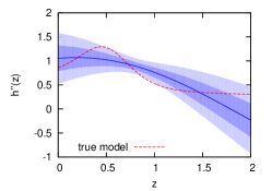
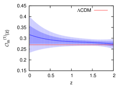
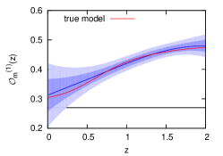
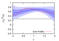
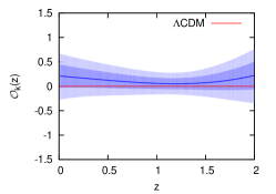
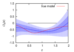
Figure 2 shows the reconstruction of . The reconstruction of and is shown in Fig. 2, and Fig. 3 gives and . We actually plot a modified which stabilises the errors at high redshift without affecting the consistency condition. The reconstructed , also requiring , is shown in Fig. 4, where we assume the concordance values and Komatsu .
Results: mock data
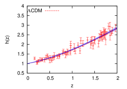
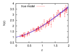
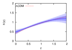
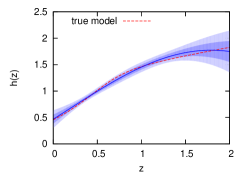
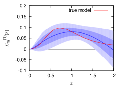
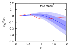
To demonstrate how a larger number of data will affect our results when reconstructing and testing CDM, we simulated a data set of 64 points for , drawing the error from a Gaussian distribution with and , adapting the methodology of Ma:2010mr .
We simulated data points for two different models:
Concordance model, , .
A model with slowly evolving equation of state:
| (10) |
and the same concordance density parameters.
Discussion
Figure 2 shows that for the CC and CC+BAO data (18 and 24 points), we get good reconstructions when there is no differentiation of involved. The BAO data set only contains 6 data points up to redshift 0.73. Beyond that redshift, the reconstruction differs significantly from CDM. The results from the CC and CC+BAO sets are however in very good agreement with CDM.
The BAO data appear to be inconsistent with the concordance model. However, 6 data points are not sufficient for a reliable reconstruction. The two data points with highest redshift happen to be below the concordance curve, which pulls the reconstructed curve down. This is probably just a coincidence, but it illustrates the importance of having the derivative of the data consistent with the model, as well as the data itself. Current and upcoming large-volume surveys, such as BOSS Schlegel:2009hj , EUCLID euclid and SKA Ansari:2011bv , will provide radial BAO measurements of increasing number and precision.
The reconstruction of and shown in Fig. 2 is more challenging for the available data set, since we need the first derivative of . With present data sets, the uncertainties in the reconstruction are quite large. Using CC and CC+BAO, these results as well as the results for and shown in Fig. 3, are consistent with CDM.
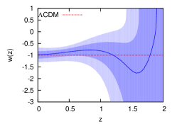
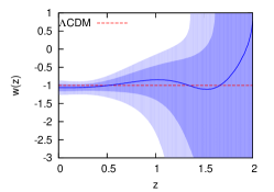
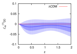
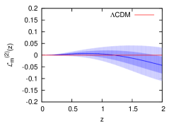
For the mock data sets, Figs. 5 and 6 show that the GP reconstructions recovers the assumed models very effectively. We can clearly distinguish the model with slowly evolving from CDM in . For and , the reconstruction errors are too large to see this difference. The same is true for consistency tests and shown in Fig. 7.
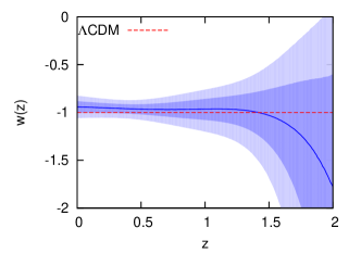
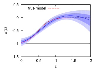
The reconstruction of the equation of state also shows a clear difference of the two models, assuming we can accurately determine , and separately from : see Fig. 8. GP works very well to recover the assumed . With less than 100 data points, we can reconstruct a dynamical dark energy model far better than is achievable using thousands of SNIa data – compare to analogous reconstructions in Seikel .
IV Conclusions
We have considered the information that current and future data can give us. Currently such data come from cosmic chronometers and BAO data, and is plainly consistent with the concordance model. Future data, however, will provide a powerful discriminator between models. It is remarkable how few data points are required compared to supernovae: to reconstruct accurately in our non-parametric way requires many thousands of SNIa, compared to less than 100 data points.
We have derived and analysed new consistency tests for the CDM model, which we have formulated in terms of directly, rather than using the more familiar distance function Clarkson:2009jq ; Clarkson (2012). By smoothing the data points using Gaussian process, we have shown that these can be very effective in determining that CDM is the incorrect model, but without having to assume the key parameters and , which currently only have constraints derived by assuming CDM or a similar alternative. These tests not only require that the data points themselves are consistent with the model, but that their derivative is also.
Future data which directly measures the expansion history will therefore play an important role in future dark energy studies.
Acknowledgements:
We thank Phil Bull and Mat Smith for discussions.
SY and RM are supported by the South African Square Kilometre Array
Project. MS and CC are supported by the National Research Foundation
(NRF) South Africa. RM is supported by the UK Science & Technology
Facilities Council (grant no. ST/H002774/1).
Appendix A Gaussian Processes
For a data set , where represents the training points , i.e. the locations of the observations, we want to reconstruct the function that describes the data at the test input points .
A Gaussian Process is a distribution over functions and is thus a generalization of a Gaussian distribution. It is defined by the mean and covariance :
| (11) |
At each , the value is drawn from a Gaussian distribution with mean and variance . and are correlated by the covariance function .
Choosing the covariance function is one of the main points for achieving satisfactory results. The squared exponential is a general purpose covariance function, which we use throughout this paper:
| (12) |
The ‘hyperparameters’ are (signal variance) and (characteristic length scale). can be thought of as the distance moved in input space before the function value changes significantly. describes the typical change in -direction. In contrast to actual parameters, they do not specify the exact form of a function, but describe typical changes in the function value.
For , the covariance matrix is given by . Then the vector with entries is drawn from a Gaussian distribution:
| (13) |
This can be considered as a prior for the distribution of . One needs to add observational information to obtain the posterior distribution.
The observational data have a covariance matrix . For uncorrelated data, is a diagonal matrix with entries . The combined distribution for and the observations is given by:
| (14) |
While the values of are already known, we want to reconstruct . Thus, we are interested in the conditional distribution
| (15) |
where
| (16) | |||
| (17) |
are the mean and covariance of , respectively. The variance of is simply the diagonal of . Equation (15) is the posterior distribution of the function given the data and the prior (13).
In order to use this equation, we need to know the values of the hyperparameters and . They can be trained by maximizing the log marginal likelihood:
| (18) | |||||
Note that this likelihood only depends on the observational data, but is independent of the locations where the function is to be reconstructed.
Derivatives of the function can be reconstructed in a similar way. For the first derivative, the conditional distribution is given by Seikel :
| (19) |
where
| (20) | |||
| (21) |
For the covariance matrices, we use the notation:
| (22) | |||||
| (23) |
is the transpose of .
To calculate a function which depends on and , we also need to know the covariances between and at each point where is to be reconstructed. This covariance is given by:
is then determined by Monte Carlo sampling, where in each step and are drawn from a multivariate normal distribution:
| (25) |
References
- (1) J. Weller and A. Albrecht, Phys. Rev. D 65, 103512 (2002)
- (2) U. Alam, V. Sahni, T. D. Saini and A. A. Starobinsky, MNRAS 344, 1057 (2003)
- (3) R. A. Daly and S. G. Djorgovski, Astrophys. J. 597, 9 (2003)
- (4) U. Alam, V. Sahni and A. A. Starobinsky, JCAP 0406, 008 (2004)
- (5) Y. Wang and M. Tegmark, Phys. Rev. Lett. 92, 241302 (2004)
- (6) R. A. Daly and S. G. Djorgovski, AJ 612, 652 (2004)
- (7) A. Shafieloo, U. Alam, V. Sahni and A. A. Starobinsky, Mon. Not. Roy. Astron. Soc. 366, 1081 (2006)
- (8) V. Sahni and A. Starobinsky, Int. J. Mod. Phys. D 15, 2105 (2006)
- (9) C. Zunckel and R. Trotta, Mon. Not. Roy. Astron. Soc. 380, 865 (2007)
- (10) C. Espana-Bonet and P. Ruiz-Lapuente, JCAP 0802, 018 (2008)
- (11) C. R. Genovese, P. Freeman, L. Wasserman, R. C. Nichol and C. Miller, arXiv:0805.4136.
- (12) C. Bogdanos and S. Nesseris, JCAP 0905, 006 (2009)
- (13) C. Clarkson and C. Zunckel, Phys. Rev. Lett. 104, 211301 (2010)
- (14) T. Holsclaw, U. Alam, B. Sanso, H. Lee, K. Heitmann, S. Habib and D. Higdon, Phys. Rev. Lett. 105, 241302 (2010)
- (15) R. G. Crittenden, G. -B. Zhao, L. Pogosian, L. Samushia and X. Zhang, JCAP 1202, 048 (2012)
- (16) A. Shafieloo, arXiv:1204.1109.
- (17) R. Lazkoz, V. Salzano and I. Sendra, arXiv:1202.4689 [astro-ph.CO].
- (18) A. Shafieloo, A. G. Kim and E. V. Linder, arXiv:1204.2272.
- (19) M. Seikel, C. Clarkson and M. Smith, arXiv:1204.2832.
- (20) C. Ma and T. -J. Zhang, Astrophys. J. 730, 74 (2011)
- (21) D. Stern, R. Jimenez, L. Verde, M. Kamionkowski and S. A. Stanford, JCAP 1002, 008 (2010)
- (22) M. Hicken et al., Astrophys. J. 700, 1097 (2009)
- Clarkson (2012) C. Clarkson, arXiv:1204.5505.
- (24) C. Rasmussen and C. Williams, Gaussian Processes for Machine Learning (MIT Press, 2006).
- (25) D. MacKay, Information Theory, Inference and Learning Algorithms (Cambridge University Press, 2003).
- (26) C. Clarkson, M. Cortes and B. A. Bassett, JCAP 0708, 011 (2007)
- (27) R. Hlozek, M. Cortes, C. Clarkson and B. Bassett, arXiv:0801.3847.
- (28) M. Kunz, arXiv:1204.5482 [astro-ph.CO].
- (29) C. Zunckel and C. Clarkson, Phys. Rev. Lett. 101, 181301 (2008)
- (30) V. Sahni, A. Shafieloo and A. A. Starobinsky, Phys. Rev. D 78 (2008) 103502
- (31) A. Shafieloo and C. Clarkson, Phys. Rev. D 81, 083537 (2010)
- (32) C. Clarkson, AIP Conf. Proc. 1241, 784 (2010)
- (33) R. Jimenez and A. Loeb, Astrophys. J. 573, 37 (2002)
- (34) S. M. Crawford, A. L. Ratsimbazafy, C. M. Cress, E. A. Olivier, S-L. Blyth and K. J. van der Heyden, arXiv:1004.2378.
- (35) M. Moresco, A. Cimatti, R. Jimenez, L. Pozzetti, G. Zamorani, M. Bolzonella, J. Dunlop and F. Lamareille et al., arXiv:1201.3609.
- (36) M. Moresco, L. Verde, L. Pozzetti, R. Jimenez and A. Cimatti, arXiv:1201.6658.
- (37) E. Gaztanaga, A. Cabre and L. Hui, Mon. Not. Roy. Astron. Soc. 399, 1663 (2009)
- (38) C.-H. Chuang and Y. Wang, arXiv:1102.2251.
- (39) C. Blake, S. Brough, M. Colless, C. Contreras, W. Couch, S. Croom, D. Croton and T. Davis et al., arXiv:1204.3674.
- (40) E. Komatsu et al., Astrophys. J. Suppl. 192, 18 (2011) [arXiv:1001.4538].
- (41) D. Schlegel et al., arXiv:0902.4680.
- (42) W. Percival, sci.esa.int/science-e/www/object/ doc.cfm?fobjectid=46450
- (43) R. Ansari, J. E. Campagne, P. Colom, J. M. L. Goff, C. Magneville, J. M. Martin, M. Moniez and J. Rich et al., arXiv:1108.1474 [astro-ph.CO].