Storrs, CT 06269-3046, USAbbinstitutetext: RIKEN-BNL Research Center, Brookhaven National Laboratory,
Upton, NY 11973, USAccinstitutetext: II. Institut für Theoretische Physik, Universität Hamburg,
Luruper Chaussee 149, 22761, Hamburg, Germanyddinstitutetext: Institut de Théorie des Phénomènes Physiques,
École Polytechnique Fédérale de Lausanne, CH-1015 Lausanne, Switzerland
Higgs boson mass and new physics
Abstract
We discuss the lower Higgs boson mass bounds which come from the absolute stability of the Standard Model (SM) vacuum and from the Higgs inflation, as well as the prediction of the Higgs boson mass coming from asymptotic safety of the SM. We account for the 3-loop renormalization group evolution of the couplings of the Standard Model and for a part of two-loop corrections that involve the QCD coupling to initial conditions for their running. This is one step above the current state of the art procedure (“one-loop matching–two-loop running”). This results in reduction of the theoretical uncertainties in the Higgs boson mass bounds and predictions, associated with the Standard Model physics, to . We find that with the account of existing experimental uncertainties in the mass of the top quark and (taken at level) the bound reads (equality corresponds to the asymptotic safety prediction), where . We argue that the discovery of the SM Higgs boson in this range would be in agreement with the hypothesis of the absence of new energy scales between the Fermi and Planck scales, whereas the coincidence of with would suggest that the electroweak scale is determined by Planck physics. In order to clarify the relation between the Fermi and Planck scale a construction of an electron-positron or muon collider with a center of mass energy (Higgs and t-quark factory) would be needed.
Keywords:
Higgs Physics, Standard Model, Renormalization Group1 Introduction
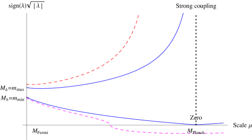
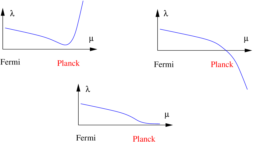
The mass of the Higgs boson in the Standard Model is an important indicator of the presence of new energy scales in particle physics. It is well known that if then the SM is a consistent effective field theory all the way from the Fermi scale up to the (reduced) Planck scale . The upper limit comes from the requirement that the Landau pole in the scalar self-coupling111To be more precise, the scalar self-coupling is infinite in the one-loop approximation only. If higher order terms are included, it may not become infinite, but move away from the region of the weak coupling. must not appear at energies below [1, 2, 3]. The lower limit comes from the requirement of the stability of the SM vacuum against tunneling to the states with the Higgs field exceeding substantially the electroweak value [4, 5, 6] (see Fig. 1).
The estimates of give a number around [1, 2, 3, 7] which is in the range excluded (at least in the range ) by the searches for the SM Higgs boson at the LHC and Tevatron [8, 9]. In other words, we already know that the SM is a weakly coupled theory up to the Planck scale.
One can distinguish between two types of the stability bounds. If , the electroweak vacuum is absolutely stable, whereas if , then it is metastable with the life-time exceeding that of the Universe. Numerically, [10]. The existence of the Higgs boson with the mass smaller than would provide an undisputed argument in favor of existence of new physics between the Fermi and Planck scale. However, already since LEP we know that this is not the case.
The Higgs mass is not at all special from the point of view of the validity of the SM up to the Planck scale. The value of , however, plays a crucial role if the Standard Model is embedded to a bigger picture which includes gravity. First, only if , the Higgs boson of the SM can play the role of the inflaton and make the Universe flat, homogeneous and isotropic, and produce a necessary spectrum of perturbations needed for structure formation [11, 12]. Second, is a prediction of asymptotically safe scenario for the SM [13], making it consistent up to arbitrary large scale.
Thus, we will focus on the upgrade of existing computations of and on the discussion of the significance of the relation between the Higgs boson (to be discovered yet) mass and for beyond the SM (BSM) physics.
The computation of has been already done in a large number of papers [14, 15, 16, 10, 12, 17]. It is divided into two parts. The first one is the determination of the parameters from the physical observables and the second one is the renormalization group running of the constants from the electroweak to a high energy scale. The most advanced recent works [10, 12, 17, 18] use the so-called “one-loop-matching–two-loop-running” procedure. It can determine the Higgs boson mass bounds with the theoretical accuracy of (see the discussion of uncertainties in [12] and below). Meanwhile, the most important terms in the 3-loop running of the gauge and Higgs coupling constants were computed in [19, 20] (we thank K. Chetyrkin and M. Zoller for sharing these results with us prior to publication). The present work accounts for corrections in the -pole matching procedure, which were not known previously. This allows us to decrease the theoretical uncertainties in the Higgs boson mass prediction/bounds, associated with the SM physics down to . This is a new result, based on a superior partial “two-loop-matching–three-loop-running” procedure. These findings are described in Section 2.2. We will see that the experimental errors in the mass of the top-quark and in the value of the strong coupling constant are too large to settle up the question of the stability of the electroweak vacuum, even if the LHC will confirm the evidence for the Higgs signal presented by the ATLAS and CMS collaborations [9, 8] in the region .
In Section 3 we will discuss the significance of the relationship between the true Higgs boson mass and for BSM physics. We will argue that if then the electroweak symmetry breaking is likely to be determined by Planck physics and that this would indicate an absence of new energy scales between the Fermi and gravitational scales. We will also address here the significance of for the SM with gravity included. Of course, this can only be done under certain assumptions. Specifically, we will discuss the non-minimal coupling of the Higgs field to the Ricci scalar (relevant for Higgs-inflation [11, 21, 12]) and the asymptotic safety scenario for the SM [13].
In Section 4 we present our conclusions. We will argue that if only the Higgs boson with the mass around and nothing else will be found at the LHC, the next step in high energy physics should be the construction a new electron-positron (or muon) collider—the Higgs and t-factory. It will not only be able to investigate in detail the Higgs and top physics, but also elucidate the possible connection of the Fermi and Planck scales.
Appendix A contains a full set of formulas required for the determination of the coupling constants from the pole masses of the SM particles, including the corrections of the orders of up to , , and . The computer code for the matching is made publicly available at http://www.inr.ac.ru/~fedor/SM/.
2 The stability bound
The stability bound will be found in the “canonical” SM, without any new degrees of freedom or any extra higher dimensional operators added, see Fig. 2.
2.1 The benchmark mass
It will be convenient for computations to introduce yet another parameter, “benchmark mass”, which we will call (without any superscript). Suppose that all parameters of the SM, except for the Higgs boson mass, are exactly known. Then , together with the normalisation point , are found from the solution of two equations:
| (1) |
where is the -function governing the renormalisation group (RG) running of . Here we define all the couplings of the SM in the renormalisation scheme which is used de-facto in the most of the higher-loop computations. Clearly, if any other renormalization scheme is used, the equations will give another benchmark mass, since the definition of all the couplings are scheme dependent.
The procedure of computing is very clean and transparent. Take the standard definition of all coupling constants of the SM, fix all of them at the Fermi scale given the experimentally known parameters such as the mass of the top quark, QCD coupling, etc., and consider the running Higgs self-coupling depending on the standard t’Hooft-Veltman parameter . Then, adjust in such a way that equations (1) are satisfied at some .
For the stability bound one should find the effective potential and solve the equations
| (2) |
where corresponds to the SM Higgs vacuum, and correspond to the extra vacuum states at large values of the scalar field. Though the effective potential and the field are both gauge and scheme dependent, the solution for the Higgs boson mass to these equations is gauge and scheme invariant.
In fact, is very close to . Numerically, the difference between them is much smaller, than the current theoretical and experimental precisions for , see below. The following well known argument explains why this is the case. The RG improved effective potential for large can be written as [22, 15, 16]
| (3) |
where is here the common name for all the SM coupling constants (which are rather small at Planck scale), and are the masses of different particles in the background of the Higgs field. If corrections are neglected, the equations (2) coincide with (1), meaning that . The numerical evaluation for one loop effective potential gives , which can be neglected in view of uncertainties discussed below.
Note that in many papers the stability bound is shown as a function of the cutoff scale (the energy scale up to which the SM can be considered as a valid effective field theory). It is required that for all . This can be reformulated as for all with pretty good accuracy. Interestingly, if , this bound is very close to the stability bound following from eq. (2), having nothing to do with the Planck scale (see also below). Note also that the uncertainties in experimental determinations of and together with theoretical uncertainties, described in the next section, lead to significant changes in the scale . Fig. 1 illustrates that for Higgs boson masses GeV this scale may vary from up to infinity within currently available precisions.
2.2 Value of
The state of art computation of contained up to now the so called one-loop -pole matching, relating the experimentally measured physical parameters to the parameters of the SM in the subtraction scheme (to be more precise, the two-loop corrections to the top pole mass– mass relation has been included [10]). Then the results of the first step are plugged into two-loop RG equations and solved numerically.
Before discussing the upgrade of the one-loop-matching–two-loop-running procedure, we will remind of the results already known and their uncertainties. We will make use of our computations of presented in [12].222The main interest in this paper was the lower bound on the Higgs boson mass in the Higgs-inflation, see below. However, has been estimated as well as a by-product of the computation. A somewhat later papers [23, 17, 18] contains exactly the same numbers for (note, however, that the theoretical uncertainties were not discussed in [23]). See also earlier computations in [14, 15, 16, 7, 10, 18].
In [12] we found:
| (4) |
and estimated the theoretical uncertainties as summarized in Table 1 (see also [17]).333The reader not interested in details of the comparison with the previous results can skip this discussion and restart at the following paragraph. While repeating this analysis we found some numerical errors which are given at the bottom section of this table (see a detailed discussion below). In total, they shift the value given in eq. (4) up by . As for uncertainties, they were estimated as follows. The one-loop matching formulas can be used directly at , or at some other energy scale, e.g. at , and then the coupling constants at can be derived with the use of RG running. The difference in procedures gives an estimate of two-loop effects in the matching procedure. This is presented by the first two lines in Table 1 (in fact, we underestimated before the uncertainty from matching—previously we had here and now ). The next two lines are associated with 3 and 4-loop corrections to the top Yukawa . The 3-loop corrections were computed in [24, 25, 26] and the four-loop contribution to the top mass was guessed to be of the order in [27, 28]. The non-perturbative QCD effects in the top pole mass– mass matching are expected to be at the same level [29, 30, 31]. For 3-loop running we put the typical coefficients in front of the largest couplings and . If these uncertainties are not correlated and can be summed up in squares, the theoretical uncertainty is . If they are summed up linearly, then the theoretical error can be as large as .
| Source of uncertainty | Nature of estimate | , GeV |
|---|---|---|
| 2-loop matching | Sensitivity to | 1.7 |
| 2-loop matching | Sensitivity to | 0.6 |
| 3-loop to | known | 1.4 |
| 4-loop to | educated guess [27, 28] | 0.4 |
| confinement, | educated guess | 0.5 |
| 3-loop running | educated guess | 0.8 |
| total uncertainty | sum of squares | 2.5 |
| total uncertainty | linear sum | 5.4 |
| Corrections to [12] | , GeV | |
| Typos in the code used in [12] | error | +0.2 |
| Extra in (A.5) of [10] | error | +0.4 |
| “Exact” formula instead of | ||
| approximation (2.20) in [32] | clarification | +0.1 |
| Total correction to (7.1) of [12] | +0.7 | |
| Total shift to be applied to (7.1) of [12] for comparison | +0.7 | |
Now, this computation can be considerably improved. First, in [19] the 3-loop corrections to the running of all gauge couplings has been calculated. Second, in [20] the leading contributions (containing the top Yukawa and ) to the running of the top quark Yukawa and the Higgs boson self coupling have been determined. This removes the uncertainty related to 3-loop RG running. In addition, in the present paper, we determine the two-loop corrections of the order of to the matching of the pole masses and the top quark Yukawa and Higgs boson self coupling constants. Also, the known [24, 25, 26] three loop QCD correction to the top quark mass relation of the order can be included (previously it had been used for estimates of uncertainties). All this considerably decreases the theoretical uncertainties in .
The individual contributions of the various new corrections on top of the previous result are summarized in the Table 2. It is clearly seen that there are two new significant contributions—one is the three-loop pure QCD correction to the top quark mass [24, 25, 26], and another is the two loop correction to the Higgs boson mass, found in the present paper. Together the new contributions sum to the overall shift of the previous prediction [12] by , giving the result444Note, that this value is the benchmark mass defined by eq. (1). The mass, corresponding to the metastability bound (2) is smaller.
| (5) |
| Contribution | , GeV |
|---|---|
| Three loop beta functions | -0.23 |
| -1.15 | |
| -0.13 | |
| 0.62 |
The new result (5) is less than away from the old one (4) if the same central values for and are inserted. This coincidence is the result of some magic. In the old evaluation several mistakes were present, summarized in Table 1. The largest one was the double counting of in (A.5) of [10], as compared to the original result [32]. Also, there were minor typos in the computer code for the matching of the Higgs coupling constant, and finally there was a small correction coming from the use of an approximate rather than exact one loop formula for corrections from [32]. These corrections add to the original number in [12]. By chance this almost exactly canceled the contribution from the higher loops, Table 2, nearly leading to a coincidence of (5) and (4).
Table 3 summarizes the uncertainties in the new computation. It contains fewer lines. Now we can ignore safely the error from higher order (4-loop) RG corrections for the running up to the Planck scale. The first two lines were derived in the same manner as previously. For the Higgs boson self-coupling we can use the matching formulas (A.46) to get the value of at scale directly, or to get the value and then evolve the constants to the scale with the RG equations. The obtained difference corresponds to the error . A similar procedure of comparing evolution between and using RG equations and direct matching formulas to the order leads for the chang in the top quark Yukawa , leading to . Note, however, that strictly speaking this test verifies the error of the dependent terms in the matching formulas, while the constant ones may lead to larger contributions. We also do not estimate now the contributions of the order , where formal order in may correspond to . Thus, this estimate should be better considered as a lower estimate of the error. The 4-loop matching and confinement contributions are the same as before.
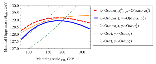
As an indication of the dependence on the matching point we present Fig. 3, where the reference Higgs boson mass was obtained using the matching formulas at scale varying between the Z-boson and top quark masses. One can see that the overall change of the Higgs boson mass is about GeV.
| Source of uncertainty | Nature of estimate | , GeV |
|---|---|---|
| 3-loop matching | Sensitivity to | 1.0 |
| 3-loop matching | Sensitivity to | 0.2 |
| 4-loop to | educated guess [27, 28] | 0.4 |
| confinement, | educated guess | 0.5 |
| 4-loop running | educated guess | |
| total uncertainty | sum of squares | 1.2 |
| total uncertainty | linear sum | 2.3 |
If we assume that these uncertainties are not correlated and symmetric we get a theoretical error in the determination of the critical Higgs boson mass . If they are summed up linearly, we get an error of . We leave it to the reader to decide which estimate of the uncertainties is more adequate. The precision of the theoretical value of can be further increased by computing the two-loop corrections to the matching procedure. Numerically, the most important terms are those when corresponds to and .
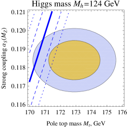
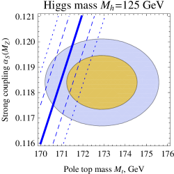
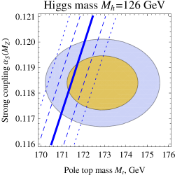
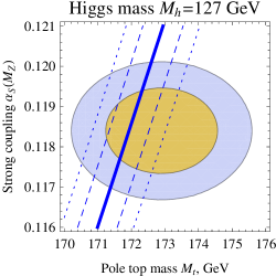
The result (5) is visualized by Fig. 4. The experimentally allowed regions for the top mass and strong coupling are adopted PDG 2010 edition [33].555Note however, that the current experimental error estimate is based on averaging over different experimental approaches. In some methods quite a different central values are obtained. See e.g. [34, 35, 36] about determination and [37, 38, 39] about . On top of these allowed regions the bands corresponding to the reference values of the Higgs boson mass being equal to are shown, with the dashed and dotted lines corresponding to quadratically or linearly added estimates of theoretical uncertainties.
One can see that the accuracy of theoretical computations and of the experimental measurements of the top and the Higgs boson masses does not allow yet to conclude with confidence whether the discovery of the Higgs boson with the mass would indicate stability or metastability of the SM vacuum. All these reference values of Higgs masses are compatible within with current observations.
3 and BSM physics
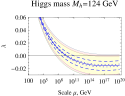
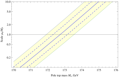
Our definition of the “benchmark” Higgs boson mass consists of the solution of the two equations (1) and gives, in addition to , the value of the scale at which the scalar self-coupling and its -function vanish simultaneously. The central value for is and is quite stable if and are varied in their confidence intervals (see Fig. 5). One can see that there is a remarkable coincidence between and the (reduced) Planck scale . The physics input in the computation of includes the parameters of the SM only, while the result gives the gravity scale. A possible explanation may be related to the asymptotic safety of the SM, see [13] and below.666Of course, this is not the only way to predict the Higgs boson mass close to . Cf. the “multiple point principle” of [40, 41], requiring the degeneracy between the SM vacuum and an extra one appearing at the Planck scale, the inflation from false vacuum decay [42, 43, 44, 45], etc. It remains to be seen if this is just the random play of the numbers or a profound indication that the electroweak symmetry breaking is related to Planck physics. If real, this coincidence indicates that there should be no new energy scales between the Planck and Fermi scales, as they would remove this coincidence unless some conspiracy is taking place.
We will discuss below two possible minimal embeddings of the SM to the theory of gravity and discuss the significance of in them.
3.1 Asymptotic safety
The asymptotic safety of the SM [13], associated with the asymptotic safety of gravity [46], is strongly related to the value of the Higgs boson mass. Though General Relativity is non-renormalizable by perturbative methods, it may exist as a field theory non-perturbatively, exhibiting a non-trivial ultraviolet fixed point (for a review see [47]). If true, all other coupling of the SM (including the Higgs self-interaction) should exhibit an asymptotically safe behaviors with the gravity contribution to the renormalisation group running included.
The prediction of the Higgs boson mass from the requirement of asymptotic safety of the SM is found as follows [13]. Consider the SM running of the coupling constants and add to the -functions extra terms coming from gravity, deriving their structure from dimensional analysis:
| (6) |
where , , , , and are some constants (anomalous dimensions) corresponding to the gauge couplings of the SM , , , the top Yukawa coupling , and the Higgs self-coupling . In addition,
| (7) |
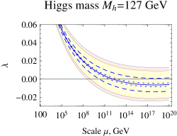
is the running Planck mass with following from numerical solutions of functional RG equations [48, 49, 50]. Now, require that the solution for all coupling constants is finite for all and that is always positive. The SM can only be asymptotically safe if , , , are all negative, leading to asymptotically safe behavior of the gauge and Yukawa couplings. For we are getting the interval of admissible Higgs boson masses, . However, if , as follows from computations of [49, 50], only one value of the Higgs boson mass leads to asymptotically safe behavior of . As is explained in [13], this behavior is only possible provided and . And, due to miraculous coincidence of and , the difference is extremely small, of the order . The evolution of the Higgs self-coupling for the case of is shown in Fig. 6, and for the case in Fig. 7.
In fact, in the discussion of the asymptotic safety of the SM one can consider a more general situation, replacing the Planck mass in eq. (7) by some cutoff scale . Indeed, if the Higgs field has non-minimal coupling with gravity (see below), the behavior of the SM coupling may start to change at energies smaller than by a factor , leading to an expectation for the range of as . Still, the difference between and remains small even for , where , making the prediction sufficiently stable against specific details of Planck physics within the asymptotic safety scenario.

3.2 and cosmology
It is important to note that if the mass of the Higgs boson is smaller than the stability bound , this does not invalidate the SM. Indeed, if the life-time of the metastable SM vacuum exceeds the age of the Universe (this is the case when , with [10]) then finding a Higgs boson in the mass interval would simply mean that we live in the metastable state with a very long lifetime. Of course, if the Higgs boson were discovered with a mass below , this would prove that there must be new physics between the Fermi and Planck scales, stabilizing the SM vacuum state. However, the latest LEP results, confirmed recently by LHC, tell us that in fact , and, therefore, that the presence of a new energy scale is not required, if only the metastability argument is used.
The bound can be strengthened if thermal cosmological evolution is considered [10]. After inflation the universe should find itself in the vicinity of the SM vacuum and stay there till present. As the probability of the vacuum decay is temperature dependent, the improved Higgs boson mass bound is controlled by the reheating temperature after inflation (or maximal temperature of the Big Bang). The latter is model dependent, leading to the impossibility to get a robust bound much better than . For example, in inflation [51, 52] the reheating temperature is rather low, [52], leading to the lower bound [53] on the Higgs boson mass, which exceeds only by .
However, if no new degrees of freedom besides those already present in the SM are introduced and the Higgs boson plays the role of inflaton, the bound reappears, as is discussed below.
3.3 Higgs inflation
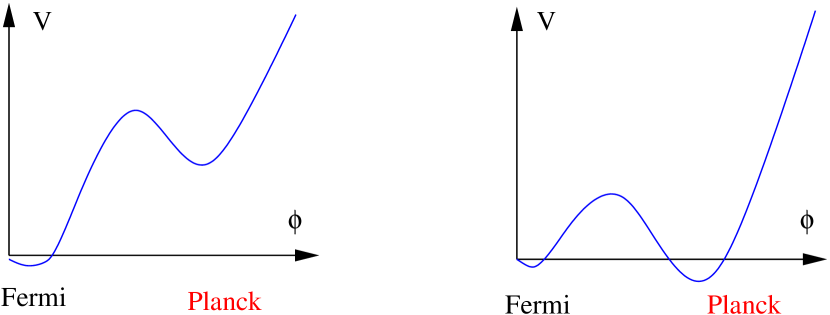
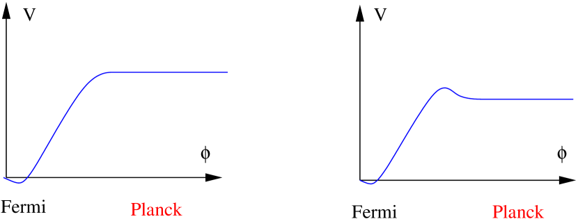
The inclusion of a non-minimal interaction of the Higgs field with gravity, given by the Lagrangian , where is the Ricci scalar, changes drastically the behavior of the Higgs potential in the region of large Higgs fields [11]. Basically, the potential becomes flat at , keeping the value it acquired at . This feature leads to a possibility of Higgs-inflation: if the parameter is sufficiently large, , [12] the Higgs boson of the SM can make the Universe flat, homogeneous and isotropic, and can produce the necessary spectrum of primordial fluctuations. The possibility of the Higgs inflation is also strongly related to the value of the Higgs boson mass: the successful inflation can only occur if . The upper limit comes from the requirement of the validity of the SM up to the inflation scale . Near the behavior of the effective potential in the Einstein frame changes as shown in Fig. 8: if the “bump” in the Higgs potential prevents the system to go to the SM vacuum state. As in the previous case, these bounds can be formulated with the use of the Higgs self-coupling . Basically, it must be perturbative and positive for all energy scales below . Though any Higgs boson mass in the interval can lead to successful inflation, the value is somewhat special. For the lower part of the admitted interval the value of the non-minimal coupling reaches its minimal value , extending the region of applicability of perturbation theory [12, 54, 55].
The computation of the lower bound on the Higgs boson mass from inflation is more complicated. It is described in detail in [21, 12]. Basically, one has to compute the Higgs potential in the chiral electroweak theory associated with large values of the Higgs field and find when the slow-roll inflation in this potential can give the large-scale perturbations observed by the COBE satellite. The outcome of these computations, however, can be formulated in quite simple terms: for inflationary bound find from the condition for all [12]. A priori, the inflationary bound could have been very different from and thus from . Indeed, both and know nothing about the Planck scale and are defined entirely within the SM, whereas the inflationary bound does use . However, the remarkable numerical coincidence, between and , makes and practically the same. The coupling constant evolves very slowly near the Planck scale, so that the regions for the Higgs boson mass following from the conditions for and are almost identical. This leads to the result that . This number is derived within the SM without addition of any higher dimensional operators.
One must note, that simple scale analysis leads to the unitarity violation in the Higgs inflation below the Planck energy scale [56, 57, 58, 59]. This means, that calculations in the Higgs inflationary models should be done with some additional assumptions about the high energy physics, formulated in [54], specifically the approximate scale invariance at high field backgrounds. As is explained in [54], adding to the SM higher-dimensional operators with a Higgs-field dependent cutoff modifies the lower bound on the Higgs boson mass in Higgs inflation. If these operators are coming with “natural” power counting coefficients (for exact definition see [54]) the sensitivity of the Higgs boson mass bound to unknown details of ultraviolet physics is rather small [54]. At the same time, it is certainly not excluded that the change of can be larger.
4 Conclusions
If the SM Higgs boson will be discovered at LHC in the remaining mass interval not excluded at 95% [9, 8], there is no necessity for a new energy scale between the Fermi and Planck scales. The EW theory remains in a weakly coupled region all the way up to , whereas the SM vacuum state lives longer than the age of the Universe. If the SM Higgs boson mass will be found to coincide with given by (5), this would put a strong argument in favor of the absence of such a scale and indicate that the electroweak symmetry breaking may be associated with the physics at the Planck scale.
The experimental precision in the Higgs boson mass measurements at the LHC can eventually reach and thus be much smaller than the present theoretical () and experimental (, ) uncertainties in determination of . The largest uncertainty comes from the measurement of the mass of the top quark. It does not look likely that the LHC will substantially reduce the error in the top quark mass determination. Therefore, to clarify the relation between the Fermi and Planck scales a construction of an electron-positron or muon collider with a center-of-mass energy of (Higgs and t-quark factory) would be needed. This would be decisive for setting up the question about the necessity for a new energy scale besides the two ones already known—the Fermi and the Planck scales. In addition, this will allow to study in detail the properties of the two heaviest particles of the Standard Model, potentially most sensitive to any types on new physics.
Surely, even if the SM is a valid effective field theory all the way up the the Planck scale, it cannot be complete as it contradicts to a number of observations. We would like to use this opportunity to underline once more that the confirmed observational signals in favor of physics beyond the Standard Model which were not discussed in this paper (neutrino masses and oscillations, dark matter and baryon asymmetry of the Universe) can be associated with new physics below the electroweak scale, for reviews see [60, 61] and references therein.777As for the dark energy, it may be related to a massless dilaton realizing spontaneously broken scale invariance [62, 63]. The minimal model—MSM, contains, in addition to the SM particles, three relatively light singlet Majorana fermions. These fermions could be responsible for neutrino masses, dark matter and baryon asymmetry of the Universe. The MSM predicts that the LHC will continue to confirm the Standard Model and see no deviations from it. At the same time, new experiments at the high-intensity frontier, discussed in [64], may be needed to uncover the new physics below the Fermi scale. In addition, new observations in astrophysics, discussed in [61], may shed light to the nature of Dark Matter. As the running of couplings in the MSM coincides with that in the SM, all results of the present paper are equally applicable to the MSM.
Acknowledgements
The work of M.S. has been supported by the Swiss National Science Foundation. The work of M.Yu.K. and B.A.K. was supported in part by the German Federal Ministry for Education and Research BMBF through Grants No. 05 HT6GUA, 05 HT4GUA/4 by the German Research Foundation DFG through the Collaborative Research Centre No. 676 Particles, Strings and the Early Universe—The Structure of Matter and Space Time, and by the Helmholtz Association HGF through the Helmholtz Alliance Ha 101 Physics at the Terascale. We thank A. Boyarsky, K. Chetyrkin, D. Gorbunov, F. Jegerlehner, G. Passarino, O. Ruchayskiy, and M. Zoller for helpful discussions, collaboration and interest to our work. M.Yu.K. is indebted to Fred Jegerlehner for a fruitful long time collaboration on developing and study scheme beyond one-loop order in framework of quantum field models with spontaneously symmetry breaking, and in particular for collaboration on [65], the results and methods of which were heavily used in the present work.
4.1 Note added
After our paper was submitted to the electronic preprint archive arXiv (on May 13) a number of events happened, which require its update. First, extra corrections to the matching procedure at low energy scale, not computed in our work, were found in [119] (May 29).888Preliminary results of Ref. [119] were presented in Ref. [118]. However, the threshold correction to the Higgs self-coupling is not specified in Ref. [118], but is presented here for the first time. Moreover, the conclusions reached in Ref. [118] disagree with ours. Ref. [119] finds agreement with our results on the order in the Higgs self-coupling constant. In addition, this paper computed a part of the corrections to the top Yukawa and Higgs coupling constants in the “gauge-less” limit of the Standard model, i.e. the two-loop terms containing the top Yukawa and scalar self-coupling were accounted for. The overall effect of these terms happened to be quite small. The corrections shift the benchmark Higgs mass up by 0.2 GeV, and reduce the sensitivity of the results to the normalisation point from 1.2 GeV to 0.8 GeV, decreasing somewhat the theoretical error-bars, see Fig. 3.
Second, the discovery of the Higgs-like resonance was announced at CERN by ATLAS and CMS collaborations [66, 67]. According to CMS,
| (8) |
while ATLAS gives a slightly higher value
| (9) |
And, finally, an updated results on the mass of the top quark were announced at ICHEP 2012 (July 9), see [68, 38]. The combination of the Tevatron results reads:
| (10) |
whereas the present LHC value is
| (11) |
The central values of the top mass are somewhat higher (by 0.3–0.4 GeV) than those which were given by the Particle Data Group at the time we were writing our paper.
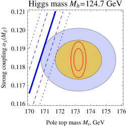
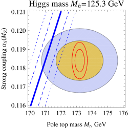
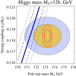
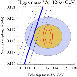
In Fig. 9, which is an update of Fig. 4, we show the changes due to the experimental shift of the top mass (we take the Tevatron result as having smaller errors) and due to the additional two-loop corrections found in [119] for the ATLAS and CMS values of the Higgs mass. The value of the benchmark Higgs mass is inside contours on the plane for the Atlas and CMS values of , entering the contours if theoretical uncertainties are incorporated. The red curves show the shrinking the size of uncertainties in and (1 and ) which can be achieved with an collider operated as a in factory on a lepton collider (this estimate is taken from [69, *AguilarSaavedra:2001rg, *Abe:2001nnb, *Abe:2001npb, *Abe:2001nqa, *Abe:2001nra, *Abe:2001gc, *Djouadi:2007ik] and [77] discussing the ILC physics).
It is important also to note, that it is difficult to determine which renormalization scheme corresponds to the numerical value of quoted by experiments. The determinations by the Tevatron and LHC collaborations [68, 78] are based on Monte Carlo event generators implemented with LO hard-scattering matrix elements. Although it is plausible and likely that the experimental values thus extracted are close to the pole mass of the top quark, this is by no means guaranteed with the due theoretical rigor [79]. In fact, rigorous determinations of the top-quark pole mass from total production cross sections yield somewhat smaller values, albeit with larger errors [120, 31, 30]. For the time being, we adopt the working hypothesis that the experimental values of [78, 68] correspond to the pole mass, bearing in mind that this is probably subject to change once a proper NLO treatment of the resonating top-quark propagators is implemented.
Thus, all our considerations remain in force and call for further improvement of the theoretical computations, which should account for all corrections to the mapping procedure, and for a construction of a factory to pin down and . A recent paper [120], where uncertainties in determination and have been analyzed, reached exactly the same conclusion.
Appendix A electroweak corrections to the top Yukawa and Higgs self couplings in Standard Model
The evaluation of radiative corrections to the relations between parameters (coupling constants) and masses of particles includes two steps: evaluation of radiative corrections between the Fermi constant and its counterpart [80] (see [81, 82, 83] for recent reviews) and the evaluation of the radiative corrections between and pole masses.
The one-loop electroweak corrections to the relation between the self-coupling and the pole mass of the Higgs boson was obtained in [84] and to the relation between the Yukawa coupling and the pole mass of top quark was found in [32]. The corresponding ingredients for the 2-loop mixed electroweak-QCD corrections were evaluated in [85, 86, 87, 88, 89, 65], but has never been assembled. We performed independent (re)calculations of all and contributions. In the following we will denote the on-shell masses by capital and the masses by lowercase .
A.1 corrections to the relation between on-shell and Fermi constant
The relation between the Fermi coupling constant and the bare parameters is as follows [80]:
| (A.12) |
where includes unrenormalized electroweak corrections and are the SU(2) coupling constant and the bare boson mass (see for details [81, 82, 83]). After performing renormalization this relation has the following form:
| (A.13) |
where on the r.h.s. all masses and coupling constants are taken in the renormalization scheme. The one-loop coefficient, , is known from [80] and for , and has the following form:
| (A.14) | |||||
Here, is defined in the scheme as
| (A.15) |
where and are the U(1) and SU(2) gauge coupling constants, respectively. The matching conditions between the parameter, defined by Eq. (A.15), and its on-shell version, [80], follows from identification
| (A.16) |
where and are the pole masses of the gauge bosons (see detailed discussion in [90, 91, 92]). The evaluation of the mixed QCD-EW coefficient, , is reduced to the evaluation of the corrections to the boson self-energy at zero momenta transfer and may be written in the following way [93, 94, 95, 96, 97]:
| (A.17) | ||||
where for and we used the results999There are typos in Eq. (4.41) of [92]: in all renormalization constants, and , “” should be replaced by “” of [92] and is the number of fermion families ( is equal to in the SM).
Using the fact, that is RG invariant, i.e. , the -dependent terms in Eq. (A.17) can be evaluated explicitly from the one-loop correction and explicit knowledge of anomalous dimension . As was shown in [90, 91, 92, 98, 99], the anomalous dimension can be extracted (i) via the beta-function of the scalar self-coupling and the anomalous dimension of the mass parameter (in unbroken phase) or (ii) via the -function of the SU(2) gauge coupling and the anomalous dimension of the boson (in broken phase):
| (A.18) |
Eq. (A.13) can be written as
| (A.19) | |||||
where and the coefficients and are defined via the RG equations:
| (A.20) | |||||
| (A.21) |
with
| (A.22) |
Collecting all terms in Eq. (A.21) we get
| (A.23) |
At the end of this section we again point out that the anomalous dimension of the vacuum expectation value within the diagram technique is defined by Eq. (A.18) and it is not equal to the anomalous dimension of the scalar field as in the effective potential approach [100]. Another important property of Eq. (A.18) is the appearance of an inverse power of the coupling constant due to the explicit inclusion of the tadpole contribution. As consequence, the limit of zero Higgs mass, , does not exist within the perturbative approach. The importance of the inclusion of the tadpole contribution to restore gauge invariance of on-shell counterterms was recognized a long time ago [101] and was explicitly included in the one-loop electroweak corrections to the matching conditions [84, 32]. The RG equations for the mass parameters were discussed in [90, 91, 92, 98, 99].
A.2 corrections to the relation between the and pole masses of the top quark
The detailed discussion and explicit evaluation101010There is typo in Eq. (4.46) of [89]: the common factor was lost. The correct result is However, all plots, the Eq. (5.57) and the Maple program [102] are correct. have been presented in [89] (the results of [89] were also used for analysis of convergence of series representation of the set of Feynman Diagrams evaluated in [103, 104]). For our analysis is enough to write the following symbolic relation between the and pole masses of the top quark:
| (A.24) |
where and are defined by Eq.(5.54) or Eq.(5.57) of [89].
A.3 corrections to the relation between the and pole masses of the Higgs boson
At the two-loop level the relation between the pole and masses is defined as follows:
| (A.25) |
where the sum runs over all species of particles, , , and are the one-loop counterterms for the charges and physical masses in the scheme and after differentiation we put all parameters equal to their on-shell values. The derivatives in Eq. (A.25) correspond to the subtraction of sub-divergences. The genuine two-loop mass counterterm comes from the shift of the term. The relation between the bare and masses of the Higgs boson has the form
| (A.26) |
where is the SU(2) renormalized coupling constant.
The exact analytical result for the two-loop quark contribution to the Higgs-boson self-energy was calculated in [88, 95, 95]. The bare two loop mixed QCD-EW contribution (with explicit inclusion of the tadpole) for the quark with mass reads:
| (A.27) |
where the last terms come from the tadpole, is the dimension of space-time [105] and
| (A.28) |
In accordance with Eq. (A.25), the coefficient of order relating the pole and masses of the Higgs boson, , can be written as
| (A.29) | |||
where
As result of our calculation we find:
| (A.31) |
The contributions of other quarks with non-zero mass are additive. Exploring the expansion for the master integral from [106], we have for t-quark contribution :
| (A.32) |
where
| (A.33) |
and we have introduced the two functions and (see also [87, 88]) defined as111111We cross checked, that Eq. (A.32) minus tadpole contribution coincides with results of Ref. [87, 95, 96, 97] after the following substitutions: (A.34)
| (A.35) |
and
| (A.36) |
In Eq. (A.32) we explicitly factorized the RG logarithms, and , which may be calculated also from the one-loop result and the mass anomalous dimensions (see [98, 99] for the general case). From the parametrization
| (A.37) | |||||
where , and using the fact that pole mass is RG invariant, we have:
| (A.38) | |||||
| (A.39) | |||||
| (A.40) |
where
| (A.41) |
In terms of the variable , defined by Eq. (A.33), the final result reads:
| (A.42) |
A.4 corrections to the top Yukawa and Higgs self couplings
The relation between the top Yukawa (Higgs) coupling and the Fermi constant is obtained from Eqs. (A.13), (A.24) and (A.37) as:
| (A.43) | |||||
| (A.44) |
and the relation between the Higgs coupling constant used in [84] and the parametrization of [90, 91, 92, 89] follows from the comparison of the RG functions: .
The result for the top-Yukawa coupling reads (see Eq. (21) in [65] and [107])
| (A.45) | |||
where are defined in Eq. (A.24). The result for the Higgs coupling is
| (A.46) | |||
where
and the sum runs over all quarks.
For completeness, we present also the explicit expressions for the derivatives (for , and ):
| (A.48) |
Terms of the order , in Eq. (A.45) and Eq. (A.46) correspond to [32] and [84], respectively. Terms of the order in Eq. (A.45) and Eq. (A.46) are the mixed electroweak-QCD corrections and , , are defined by Eq. (A.17), Eq. (A.32), and Eq.(5.54) or Eq.(5.57) of [89].
For completeness we present also the the coefficient . We divide all corrections into bosonic (diagrams without any fermions) and fermionic (diagrams exhibiting a fermion loop) ones: . Using the notations of [90, 91, 92] we may write the one-loop corrections in the following form
| (A.49) | |||||
where (see Eq. (E.6) in [106])
| (A.51) | |||||
with
All results are collected in the Maple code of Ref. [102].
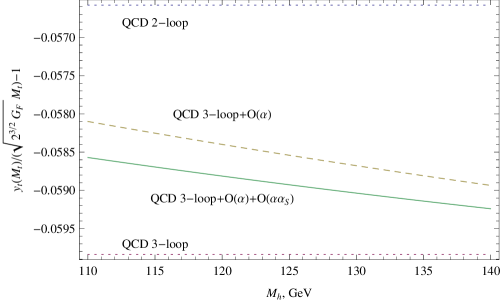
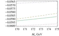
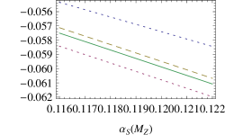
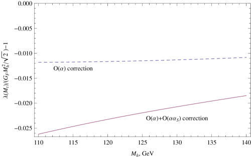
Appendix B Beta functions
Two loop SM beta functions above the top mass are collected in [10] (see [108, 109, 110, 111, 112, 113, 114, 115, 116, 117] for original works). The three loop beta functions can be read off [19, 20].
Below the top mass the one loop beta functions for the gauge couplings were used to evolve the PDG values from to . For example, for the
| (B.52) |
The higher loop corrections are not important numerically for the electroweak constants for the small energy range between and .
For the strong coupling the RG equation up to order is used
| (B.53) |
and is the number of flavors below the top quark. Strictly speaking, the value of obtained from this equation should be also shifted to the 6-quark value by
| (B.54) |
but this introduces a negligible effect () for the Higgs mass.
In all the formulas of the Appendix A we use the values of and at the matching scale .
References
- [1] L. Maiani, G. Parisi, and R. Petronzio, Bounds on the Number and Masses of Quarks and Leptons, Nucl. Phys. B136 (1978) 115.
- [2] N. Cabibbo, L. Maiani, G. Parisi, and R. Petronzio, Bounds on the Fermions and Higgs Boson Masses in Grand Unified Theories, Nucl. Phys. B158 (1979) 295–305.
- [3] M. Lindner, Implications of Triviality for the Standard Model, Zeit. Phys. C31 (1986) 295.
- [4] N. V. Krasnikov, Restriction of the fermion mass in gauge theories of weak and electromagnetic interactions, Yad. Fiz. 28 (1978) 549–551.
- [5] P. Q. Hung, Vacuum Instability and New Constraints on Fermion Masses, Phys. Rev. Lett. 42 (1979) 873.
- [6] H. D. Politzer and S. Wolfram, Bounds on Particle Masses in the Weinberg-Salam Model, Phys. Lett. B82 (1979) 242–246.
- [7] T. Hambye and K. Riesselmann, Matching conditions and Higgs mass upper bounds revisited, Phys. Rev. D55 (1997) 7255–7262, [hep-ph/9610272].
- [8] CMS Collaboration Collaboration, S. Chatrchyan et al., Combined results of searches for the standard model Higgs boson in collisions at TeV, Phys.Lett. B710 (2012) 26–48, [arXiv:1202.1488].
- [9] ATLAS Collaboration Collaboration, G. Aad et al., Combined search for the Standard Model Higgs boson using up to 4.9 fb-1 of pp collision data at TeV with the ATLAS detector at the LHC, Phys.Lett. B710 (2012) 49–66, [arXiv:1202.1408].
- [10] J. R. Espinosa, G. F. Giudice, and A. Riotto, Cosmological implications of the Higgs mass measurement, JCAP 0805 (2008) 002, [arXiv:0710.2484].
- [11] F. L. Bezrukov and M. Shaposhnikov, The Standard Model Higgs boson as the inflaton, Phys. Lett. B659 (2008) 703–706, [arXiv:0710.3755].
- [12] F. Bezrukov and M. Shaposhnikov, Standard Model Higgs boson mass from inflation: two loop analysis, JHEP 07 (2009) 089, [arXiv:0904.1537].
- [13] M. Shaposhnikov and C. Wetterich, Asymptotic safety of gravity and the Higgs boson mass, Phys. Lett. B683 (2010) 196–200, [arXiv:0912.0208].
- [14] G. Altarelli and G. Isidori, Lower limit on the Higgs mass in the standard model: An Update, Phys. Lett. B337 (1994) 141–144.
- [15] J. A. Casas, J. R. Espinosa, and M. Quiros, Improved Higgs mass stability bound in the standard model and implications for supersymmetry, Phys. Lett. B342 (1995) 171–179, [hep-ph/9409458].
- [16] J. A. Casas, J. R. Espinosa, and M. Quiros, Standard Model stability bounds for new physics within LHC reach, Phys. Lett. B382 (1996) 374–382, [hep-ph/9603227].
- [17] M. Holthausen, K. S. Lim, and M. Lindner, Planck scale Boundary Conditions and the Higgs Mass, JHEP 1202 (2012) 037, [arXiv:1112.2415].
- [18] J. Elias-Miro, J. R. Espinosa, G. F. Giudice, G. Isidori, A. Riotto, et al., Higgs mass implications on the stability of the electroweak vacuum, Phys.Lett. B709 (2012) 222–228, [arXiv:1112.3022].
- [19] L. N. Mihaila, J. Salomon, and M. Steinhauser, Gauge coupling beta functions in the standard model to three loops, Phys. Rev. Lett. 108 (2012) 151602, [arXiv:1201.5868].
- [20] K. Chetyrkin and M. Zoller, Three-loop -functions for top-Yukawa and the Higgs self-interaction in the Standard Model, JHEP 1206 (2012) 033, [arXiv:1205.2892].
- [21] F. L. Bezrukov, A. Magnin, and M. Shaposhnikov, Standard Model Higgs boson mass from inflation, Phys. Lett. B675 (2009) 88–92, [arXiv:0812.4950].
- [22] S. R. Coleman and E. Weinberg, Radiative corrections as the origin of spontaneous symmetry breaking, Phys. Rev. D7 (1973) 1888–1910.
- [23] J. Ellis, J. R. Espinosa, G. F. Giudice, A. Hoecker, and A. Riotto, The Probable Fate of the Standard Model, Phys. Lett. B679 (2009) 369–375, [arXiv:0906.0954].
- [24] K. G. Chetyrkin and M. Steinhauser, Short distance mass of a heavy quark at order , Phys. Rev. Lett. 83 (1999) 4001–4004, [hep-ph/9907509].
- [25] K. G. Chetyrkin and M. Steinhauser, The relation between the and the on-shell quark mass at order , Nucl. Phys. B573 (2000) 617–651, [hep-ph/9911434].
- [26] K. Melnikov and T. van Ritbergen, The three-loop relation between the and the pole quark masses, Phys. Lett. B482 (2000) 99–108, [hep-ph/9912391].
- [27] A. Kataev and V. Kim, Uncertainties of QCD predictions for Higgs boson decay into bottom quarks at NNLO and beyond, PoS ACAT08 (2008) 004, [arXiv:0902.1442].
- [28] A. Kataev and V. Kim, Peculiar features of the relations between pole and running heavy quark masses and estimates of the contributions, Phys.Part.Nucl. 41 (2010) 946–950, [arXiv:1001.4207].
- [29] M. C. Smith and S. S. Willenbrock, Top quark pole mass, Phys. Rev. Lett. 79 (1997) 3825–3828, [hep-ph/9612329].
- [30] A. H. Hoang, A. Jain, I. Scimemi, and I. W. Stewart, Infrared Renormalization Group Flow for Heavy Quark Masses, Phys.Rev.Lett. 101 (2008) 151602, [arXiv:0803.4214].
- [31] A. H. Hoang, A. Jain, I. Scimemi, and I. W. Stewart, R-evolution: Improving perturbative QCD, Phys.Rev. D82 (2010) 011501, [arXiv:0908.3189].
- [32] R. Hempfling and B. A. Kniehl, On the relation between the fermion pole mass and MS Yukawa coupling in the standard model, Phys.Rev. D51 (1995) 1386–1394, [hep-ph/9408313].
- [33] Particle Data Group Collaboration, K. Nakamura et al., Review of particle physics, J.Phys.G G37 (2010) 075021.
- [34] S. Alekhin, J. Blumlein, and S. Moch, Parton distribution functions and benchmark cross sections at NNLO, arXiv:1202.2281.
- [35] G. Watt, Parton distribution function dependence of benchmark Standard Model total cross sections at the 7 TeV LHC, JHEP 1109 (2011) 069, [arXiv:1106.5788].
- [36] G. Watt, MSTW PDFs and impact of PDFs on cross sections at Tevatron and LHC, arXiv:1201.1295.
- [37] U. Langenfeld, S. Moch, and P. Uwer, Measuring the running top-quark mass, Phys.Rev. D80 (2009) 054009, [arXiv:0906.5273].
- [38] Tevatron Electroweak Working Group, for the CDF and D0 Collaborations Collaboration, Combination of CDF and D0 results on the mass of the top quark using up to 5.8 fb-1 of data, arXiv:1107.5255.
- [39] D0 Collaboration Collaboration, V. M. Abazov et al., Determination of the pole and masses of the top quark from the cross section, Phys.Lett. B703 (2011) 422–427, [arXiv:1104.2887].
- [40] D. Bennett and H. B. Nielsen, Predictions for nonAbelian fine structure constants from multicriticality, Int.J.Mod.Phys. A9 (1994) 5155–5200, [hep-ph/9311321].
- [41] C. Froggatt and H. B. Nielsen, Standard model criticality prediction: Top mass GeV and Higgs mass GeV, Phys.Lett. B368 (1996) 96–102, [hep-ph/9511371].
- [42] G. Isidori, V. S. Rychkov, A. Strumia, and N. Tetradis, Gravitational corrections to standard model vacuum decay, Phys.Rev. D77 (2008) 025034, [arXiv:0712.0242].
- [43] I. Masina and A. Notari, The Higgs mass range from Standard Model false vacuum Inflation in scalar-tensor gravity, arXiv:1112.2659.
- [44] I. Masina and A. Notari, Standard Model False Vacuum Inflation: Correlating the Tensor-to-Scalar Ratio to the Top Quark and Higgs Boson masses, Phys.Rev.Lett. 108 (2012) 191302, [arXiv:1112.5430].
- [45] I. Masina and A. Notari, Inflation from the Higgs field false vacuum with hybrid potential, arXiv:1204.4155.
- [46] S. Weinberg, Ultraviolet divergences in quantum theories of gravity, in General Relativity: An Einstein centenary survey, edited by S. W.Hawking and W.Israel (Cambridge University Press) (1979) 790.
- [47] M. Niedermaier and M. Reuter, The Asymptotic Safety Scenario in Quantum Gravity, Living Rev.Rel. 9 (2006) 5.
- [48] M. Reuter, Nonperturbative evolution equation for quantum gravity, Phys.Rev. D57 (1998) 971–985, [hep-th/9605030].
- [49] R. Percacci and D. Perini, Asymptotic safety of gravity coupled to matter, Phys.Rev. D68 (2003) 044018, [hep-th/0304222].
- [50] G. Narain and R. Percacci, Renormalization Group Flow in Scalar-Tensor Theories. I, Class.Quant.Grav. 27 (2010) 075001, [arXiv:0911.0386].
- [51] A. A. Starobinsky, A new type of isotropic cosmological models without singularity, Phys. Lett. B91 (1980) 99–102.
- [52] D. Gorbunov and A. Panin, Scalaron the mighty: producing dark matter and baryon asymmetry at reheating, Phys.Lett. B700 (2011) 157–162, [arXiv:1009.2448].
- [53] F. Bezrukov and D. Gorbunov, Distinguishing between -inflation and Higgs-inflation, Phys. Lett. B713 (2011) 365, [arXiv:1111.4397].
- [54] F. Bezrukov, A. Magnin, M. Shaposhnikov, and S. Sibiryakov, Higgs inflation: consistency and generalisations, JHEP 1101 (2011) 016, [arXiv:1008.5157].
- [55] A. Barvinsky, A. Kamenshchik, C. Kiefer, A. Starobinsky, and C. Steinwachs, Asymptotic freedom in inflationary cosmology with a non-minimally coupled Higgs field, JCAP 0912 (2009) 003, [arXiv:0904.1698].
- [56] C. P. Burgess, H. M. Lee, and M. Trott, Power-counting and the Validity of the Classical Approximation During Inflation, JHEP 09 (2009) 103, [arXiv:0902.4465].
- [57] J. L. F. Barbon and J. R. Espinosa, On the Naturalness of Higgs Inflation, Phys. Rev. D79 (2009) 081302, [arXiv:0903.0355].
- [58] C. P. Burgess, H. M. Lee, and M. Trott, Comment on Higgs Inflation and Naturalness, JHEP 07 (2010) 007, [arXiv:1002.2730].
- [59] M. P. Hertzberg, On Inflation with Non-minimal Coupling, JHEP 11 (2010) 023, [arXiv:1002.2995].
- [60] M. Shaposhnikov, Is there a new physics between electroweak and Planck scales?, arXiv:0708.3550.
- [61] A. Boyarsky, O. Ruchayskiy, and M. Shaposhnikov, The role of sterile neutrinos in cosmology and astrophysics, Ann.Rev.Nucl.Part.Sci. 59 (2009) 191–214, [arXiv:0901.0011].
- [62] M. Shaposhnikov and D. Zenhausern, Scale invariance, unimodular gravity and dark energy, Phys. Lett. B671 (2009) 187–192, [arXiv:0809.3395].
- [63] M. Shaposhnikov and D. Zenhausern, Quantum scale invariance, cosmological constant and hierarchy problem, Phys. Lett. B671 (2009) 162–166, [arXiv:0809.3406].
- [64] D. Gorbunov and M. Shaposhnikov, How to find neutral leptons of the MSM?, JHEP 10 (2007) 015, [arXiv:0705.1729].
- [65] F. Jegerlehner and M. Kalmykov, relation between pole- and mass of the t quark, Acta Phys.Polon. B34 (2003) 5335–5344, [hep-ph/0310361].
- [66] ATLAS Collaboration Collaboration, G. Aad et al., Observation of a new particle in the search for the Standard Model Higgs boson with the ATLAS detector at the LHC, arXiv:1207.7214.
- [67] CMS Collaboration Collaboration, S. Chatrchyan et al., Observation of a new boson at a mass of 125 GeV with the CMS experiment at the LHC, Phys.Lett.B (2012) [arXiv:1207.7235].
- [68] T. Muller, New results from the top quark, in ICHEP 2012 Conference, Melbourne, 2012. http://indico.cern.ch/getFile.py/access?contribId=7&sessionId=17&resId=1&materialId=slides&confId=181298.
- [69] ECFA/DESY LC Physics Working Group Collaboration, E. Accomando et al., Physics with linear colliders, Phys.Rept. 299 (1998) 1–78, [hep-ph/9705442].
- [70] ECFA/DESY LC Physics Working Group Collaboration, J. Aguilar-Saavedra et al., TESLA: The superconducting electron positron linear collider with an integrated x-ray laser laboratory. technical design report. part 3. physics at an linear collider, hep-ph/0106315.
- [71] American Linear Collider Working Group Collaboration, T. Abe et al., Linear collider physics resource book for Snowmass 2001. Part 1. Introduction, hep-ex/0106055.
- [72] American Linear Collider Working Group Collaboration, T. Abe et al., Linear collider physics resource book for Snowmass 2001. Part 2. Higgs and supersymmetry studies, hep-ex/0106056.
- [73] American Linear Collider Working Group Collaboration, T. Abe et al., Linear collider physics resource book for Snowmass 2001. Part 3. Studies of exotic and standard model physics., hep-ex/0106057.
- [74] American Linear Collider Working Group Collaboration, T. Abe et al., Linear collider physics resource book for Snowmass 2001. Part 4. Theoretical, accelerator, and experimental options, hep-ex/0106058.
- [75] ACFA Linear Collider Working Group Collaboration, K. Abe et al., Particle physics experiments at JLC, hep-ph/0109166.
- [76] ILC Collaboration, G. Aarons et al., International Linear Collider Reference Design Report Volume 2: PHYSICS AT THE ILC, arXiv:0709.1893.
- [77] M. Winter, “ILC note PHSM-2001-016.” http://www-flc.desy.de/lcnotes/notes/LC-PHSM-2001-016.ps.gz.
- [78] ATLAS Collaboration, CMS Collaboration Collaboration, S. Blyweert, Top-quark mass measurements at the LHC, arXiv:1205.2175.
- [79] C. Schwanenberger, Measurements of the inclusive cross section and of differential distributions in top quark pair production (D0), in ICHEP 2012 Conference, Melbourne, 2012. https://indico.cern.ch/getFile.py/access?contribId=534&sessionId=67&resId=0&materialId=slides&confId=181298.
- [80] A. Sirlin, Radiative corrections in the SU(2)U(1) theory: A simple renormalization framework, Phys.Rev. D22 (1980) 971–981.
- [81] W. Marciano and A. Sirlin, Radiative corrections to neutrino induced neutral current phenomena in the SU(2)U(1) theory, Phys.Rev. D22 (1980) 2695. [Erratum-ibid. D 31 (1985) 213].
- [82] G. Burgers and F. Jegerlehner, or the relation between the electroweak couplings and the weak vector boson masses, Conf.Proc. C8902201 (1989) 55–88.
- [83] S. Actis and G. Passarino, Two-loop renormalization in the Standard Model part III: Renormalization equations and their solutions, Nucl.Phys. B777 (2007) 100–156, [hep-ph/0612124].
- [84] A. Sirlin and R. Zucchini, Dependence of the quartic coupling on and the possible onset of new physics in the higgs sector of the standard model, Nucl.Phys. B266 (1986) 389.
- [85] T. Chang, K. Gaemers, and W. van Neerven, QCD Corrections to the Mass and Width of the Intermediate Vector Bosons, Nucl.Phys. B202 (1982) 407.
- [86] A. Djouadi, vacuum polarization functions of the standard model gauge bosons, Nuovo Cim. A100 (1988) 357.
- [87] B. A. Kniehl, Two Loop Corrections to the Vacuum Polarizations in Perturbative QCD, Nucl.Phys. B347 (1990) 86–104.
- [88] A. Djouadi and P. Gambino, QCD corrections to Higgs boson selfenergies and fermionic decay widths, Phys.Rev. D51 (1995) 218–228, [hep-ph/9406431].
- [89] F. Jegerlehner and M. Kalmykov, correction to the pole mass of the t quark within the standard model, Nucl.Phys. B676 (2004) 365–389, [hep-ph/0308216].
- [90] F. Jegerlehner, M. Kalmykov, and O. Veretin, versus pole masses of gauge bosons: Electroweak bosonic two loop corrections, Nucl.Phys. B641 (2002) 285–326, [hep-ph/0105304].
- [91] F. Jegerlehner, M. Y. Kalmykov, and O. Veretin, Full two loop electroweak corrections to the pole masses of gauge bosons, Nucl.Phys.Proc.Suppl. 116 (2003) 382–386, [hep-ph/0212003].
- [92] F. Jegerlehner, M. Y. Kalmykov, and O. Veretin, versus pole masses of gauge bosons. 2. Two loop electroweak fermion corrections, Nucl.Phys. B658 (2003) 49–112, [hep-ph/0212319].
- [93] F. Halzen and B. A. Kniehl, beyond one loop, Nucl.Phys. B353 (1991) 567–590.
- [94] S. Fanchiotti, B. A. Kniehl, and A. Sirlin, Incorporation of QCD effects in basic corrections of the electroweak theory, Phys.Rev. D48 (1993) 307–331, [hep-ph/9212285].
- [95] B. A. Kniehl and A. Sirlin, Comparative analysis of three methods to evaluate vacuum polarization functions, Phys.Lett. B318 (1993) 367–370.
- [96] B. A. Kniehl, Two loop corrections to the fermionic decay rates of the standard model Higgs boson, Phys.Rev. D50 (1994) 3314–3322, [hep-ph/9405299].
- [97] A. Djouadi and P. Gambino, Electroweak gauge bosons selfenergies: Complete QCD corrections, Phys.Rev. D49 (1994) 3499–3511, [hep-ph/9309298].
- [98] F. Jegerlehner, M. Y. Kalmykov, and O. Veretin, Pole masses of gauge bosons: 2 loop electroweak corrections, Nucl.Instrum.Meth. A502 (2003) 618–620.
- [99] F. Jegerlehner and M. Y. Kalmykov, Steps towards full two-loop calculations for 2 fermion to 2 fermion processes: Running versus pole masses schemes, Nucl.Instrum.Meth. A534 (2004) 299–303, [hep-ph/0404213].
- [100] H. Arason, D. Castano, B. Keszthelyi, S. Mikaelian, E. Piard, et al., Renormalization group study of the standard model and its extensions. 1. The Standard model, Phys.Rev. D46 (1992) 3945–3965.
- [101] J. Fleischer and F. Jegerlehner, Radiative Corrections to Higgs Decays in the Extended Weinberg-Salam Model, Phys.Rev. D23 (1981) 2001–2026.
- [102] M. Y. Kalmykov. http://theor.jinr.ru/~kalmykov/pole/pole.html.
- [103] M. Faisst, J. H. Kuhn, and O. Veretin, Pole versus MS mass definitions in the electroweak theory, Phys.Lett. B589 (2004) 35–38, [hep-ph/0403026].
- [104] D. Eiras and M. Steinhauser, Two-loop O(alpha alpha(s)) corrections to the on-shell fermion propagator in the standard model, JHEP 0602 (2006) 010, [hep-ph/0512099].
- [105] G. ’t Hooft and M. Veltman, Regularization and Renormalization of Gauge Fields, Nucl.Phys. B44 (1972) 189–213.
- [106] A. I. Davydychev and M. Y. Kalmykov, Massive Feynman diagrams and inverse binomial sums, Nucl.Phys. B699 (2004) 3–64, [hep-th/0303162].
- [107] B. A. Kniehl, J. H. Piclum, and M. Steinhauser, Relation between bottom-quark Yukawa coupling and pole mass, Nucl.Phys. B695 (2004) 199–216, [hep-ph/0406254].
- [108] M. Fischler and J. Oliensis, Two Loop Corrections to the Evolution of the Higgs-Yukawa Coupling Constant, Phys. Lett. B119 (1982) 385.
- [109] M. Fischler and J. Oliensis, Detailed Calculation of the Complete Two Loop Higgs-Yukawa beta Function in an Arbitrary alpha Gauge, Phys.Rev. D28 (1983) 2027.
- [110] C. Ford, D. R. T. Jones, P. W. Stephenson, and M. B. Einhorn, The Effective potential and the renormalization group, Nucl. Phys. B395 (1993) 17–34, [hep-lat/9210033].
- [111] I. Jack, Two loop background field calculations for gauge theories with scalar fields, J. Phys. A16 (1983) 1083.
- [112] I. Jack and H. Osborn, General two loop beta functions for gauge theories with arbitrary scalar fields, J. Phys. A16 (1983) 1101.
- [113] I. Jack, Two loop beta functions for supersymmetric gauge theories, Phys. Lett. B147 (1984) 405.
- [114] I. Jack and H. Osborn, General background field calculations with fermion fields, Nucl. Phys. B249 (1985) 472.
- [115] M. E. Machacek and M. T. Vaughn, Two Loop Renormalization Group Equations in a General Quantum Field Theory. 1. Wave Function Renormalization, Nucl.Phys. B222 (1983) 83.
- [116] M. E. Machacek and M. T. Vaughn, Two-loop renormalization group equations in a general quantum field theory (II). Yukawa couplings, Nuclear Physics B 236 (1984) 221–232.
- [117] M. E. Machacek and M. T. Vaughn, Two-loop renormalization group equations in a general quantum field theory : (III). Scalar quartic couplings, Nuclear Physics B 249 (1985) 70–92.
- [118] A. Strumia, Higgs weights 125 GeV! Now what?, in Implications of LHC results for TeV-scale physics, (CERN), March 28, 2012. https://indico.cern.ch/getFile.py/access?contribId=47&sessionId=20&resId=0&materialId=slides&confId=162621.
- [119] G. Degrassi, S. Di Vita, J. Elias-Miro, J. R. Espinosa, G. F. Giudice, et al., Higgs mass and vacuum stability in the Standard Model at NNLO, JHEP 1208 (2012) 098, [arXiv:1205.6497].
- [120] S. Alekhin, A. Djouadi, and S. Moch, The top quark and Higgs boson masses and the stability of the electroweak vacuum, arXiv:1207.0980.