Observational Constraints on Modified Chaplygin Gas in Horava-Lifshitz Gravity
Abstract
We present Cosmological models with modified Chaplygin gas (MCG) in the framework of Horava-Lifshitz (HL) theory of gravity both with and without detailed balance. The equation of state (EOS) for a MCG contains three unknown parameters namely, , , . The allowed values of some of these parameters of the EOS are determined using the recent astrophysical and cosmological observational data. Using observational data from , BAO peak parameter, CMB shift parameter we study cosmologies in detailed-balance and beyond detailed-balance scenario. In this paper we take up the beyond detailed-balance scenario in totality and contribution of dark radiation in the case of detailed-balance scenario on the parameters of the EOS. We explore the effect of dark radiation on the whole range the of effective neutrino parameter to constrain matter contributing parameter in both the detailed-balance and the beyond-detailed balance scenario. It has been observed that greater the dark radiation less the matter contribution in the MCG in both the scenario considered here. In order to check the validity of beyond detailed balance scenario we plot supernovae magnitudes () with redshift of Union2 data and then the variation of state parameter with redshift is studied. It has been observed that beyond detailed balance scenario is equally suitable in HL gravity with MCG.
keywords:
Modified Chaplygin Gas, Horava-Lifshitz gravity, Dark energy.1 Introduction
The big-bang cosmology has become the standard model for cosmology which accommodates a beginning of the Universe at some finite past. The discovery of CMBR (Penzias, Wilson, 1965; Dicke et al., 1965) supports such model of the universe. However, big-bang cosmology based on perfect fluid assumption fails to account some of the observed facts both in the early and at late universe. The standard Big-bang model is known to have several limitations; for instance, (i) Horizon problem (ii) Flatness problem (iii) the singularity problem, to name a few. It is known that the above problems can be resolved by invoking a phase of inflation at a very early epoch. Most of these problems have, however, been resolved by invoking inflation (Guth, 1981; Linde, 1982; Albrecht & Steinhardt, 1982; Sato, 1981) in the semiclassical theory of gravity. On the other hand recent observations predict that our universe is passing through a phase of acceleration (Riess et al., 1998). This phase of acceleration is believed to be a late time phase of the universe and it comes out that such a phase cannot be accommodated in the general theory of relativity with the usual matter fields in the standard model of particle physics. Since a universe with inflation should give satisfactory explanation of what happens close to the Planck era, it is also necessary to consider a satisfactory theory which is valid near that epoch. It may be pointed out here that a quantum gravity effect becomes important at the Planck time. But a consistent theory of quantum gravity is yet to emerge. In this direction superstring theory may be considered as one of the promising candidate of quantum theory of gravity. Cosmological models are also proposed in Loop Quantum Gravity (LQG) (Bojowald, 2001) which avoids initial singularity. However, a proper description of time evolution of quantum space-time in the LQG is not satisfactory. Several attempts have been made in the recent past to achieve a complete quantum gravitational theory (UV complete theory). Among many such attempts, Horava-Lifshitz (henceforth, HL) theory of gravity appears to be interesting. The success of the Lifshitz theory in solid state physics motivated Horava to propose a theory of gravity, often called Horava-Lifshitz (HL) gravity (Horava, 2009) which may be important to explore a viable cosmological model. In the ultraviolet (UV) limit, HL gravity has a Lifshitz-like anisotropic scaling as and , between space and time, characterized by the dynamical critical exponent and thus breaks the Lorentz invariance; while in the infra-red (IR) limit, the scale reduces to . So, it is expected that it may reduce to classical general relativistic theory of gravity in the low energy limit. The Friedmann equation gets modified by a term (Lu, Mei & Pope, 2009; Calcagni, 2009; Kiritsis & Kofinas, 2009), where is the scale factor in a non-flat universe in the HL-gravity.
In the original HL gravity, Horava assumed two conditions: detailed balance and projectibility. More recently, Sotiriou, Visser and Weifurtner (SVW) (Sotiriou, Visser & Weinfurtner, 2009), proposed a general HL theory with projectability but without detailed-balance conditions. For a spatially curved Friedmann-Robertson-Walker universe, the SVW generalization yields an extra -term that modifies the coefficient of the term in the Friedmann equation as compared to the HL theory. Therefore, it is important to look for cosmological models in Horava gravity considering projectibility with and without detailed-balance.
In the HL-gravity, the initial bigbang singularity may not arise due to the presence of higher order terms in the spatial curvatures [2.1]. There are many such novel features of HL gravity for which it is worth to explore different aspects of observed universe. A volume of literature in the framework of the HL gravity appeared containing the study of gravitational wave production (Mukohyama et al., 2009; Park, 2009; Myung, 2009), perturbation spectrum (Gao et. al., 2009; Cai and Zhang, 2009; Wang and Maartens, 2010), black-hole properties (Danielsson and Thorlacius, 2009; Cai, Cao & Ohta, 2009; Kehagias & Sfetsos, 2009), dark energy phenomenology (Park, 2010; Chaichian et. al., 2010), the problems of determining observational constraints in the theory (Dutta & Saridakis, 2010), astrophysical phenomenology (Kim et. al., 2009; Harko, 2009; Iorio and Ruggiero, 2009), thermodynamical properties etc. (Wang & Wu, 2009; Cai, Cao & Ohta, 2009). Though there exists foundational and conceptual issues of Horava-Lifshitz gravity and its associated cosmology, cosmological scenario have been examined with generalised Chaplygin gas (GCG) (Ali et. al., 2010). GCG being an exotic matter may be useful to address the recent acceleration of the universe. One of the characteristic features of the GCG is that it behaves as a pressureless fluid at the early stage of the evolution of the universe, and at a later stage it behaves as a cosmological constant. Recently, a modified form of Chaplygin gas is also considered extensively in cosmology (Liu & Lu, 2005; Thakur, Ghose & Paul, 2009). The modified Chaplygin gas (MCG) is more general and contains three free parameters. The idea is to interpolate states of standard fluids at high pressures and at high energy densities to a constant negative pressure at low energy densities (Debnath, Banerjee and Chakraborty, 2004). In the present work we explore cosmological models with MCG in the framework of HL gravity and determine the range of parameters of MCG from recent cosmological observations. We examine the effect of effective neutrino parameter on both detailed-balance and beyond-detailed balance scenario. Here compatibility of beyond detailed balance scenario is also explored in details using recent observational data in HL gravity with MCG . The objective of the paper is to determine the limits of the unknown EOS parameters using the observational data. The equation of state parameter of the total cosmic fluid defined by , will be evaluated and examined at different values of redshift parameters. Comparing the supernovae magnitudes () vs. redshift () with Union2 data we test the viability of beyond-detailed balance scenario. The suitability of the model is also examined using vs. plot in our model.
The paper is organized as follows: In sec. 2, we present the basic equations for Horava-Lifshitz cosmology and obtain the Friedmann equations for detailed balance and beyond detailed balance conditions. In sec. 3, the energy density and EOS for MCG is presented. In sec. 4 , the constraints on detailed-balance condition and beyond detailed balance condition from the observations is presented. In sec. 5, numerical analysis to determine constraints on EOS parameters are obtained for detailed balance. In sec. 6, numerical analysis to determine constraints on EOS parameters are obtained for beyond detailed balance scenario. In sec. 7, the viability of MCG in HL gravity is discussed. Finally, in sec. 8, we summarize the result.
2 Horava-Lifshitz Cosmology
In Horava-Lifshitz gravity (Calcagni, 2009; Kiritsis & Kofinas, 2009), it is convenient to use the four-dimensional space-time metric of the Arnowitt-Deser-Misner (ADM) decomposition form which is given by
| (1) |
where the basic variables are lapse function , shift vector , and the spatial metric . The scaling transformation of the co-ordinates reads: and . The shift and the 3d spatial metric depend both on the time coordinate and the spatial coordinate , the lapse is assumed to depend on time only. This condition on the lapse is called the projectibility condition. The action of HL gravity consists of kinetic and potential terms as follows:
| (2) |
The kinetic term is given by
| (3) |
where is the extrinsic curvature and dot represents derivative with respect to time ().
2.1 Detailed Balance Condition and Projectibility
The symmetry property of the Lagrangian , employed in the gravitational action drastically reduces the number of invariants which one should actually consider in the action to begin with (Horava, 2009). The above symmetry is known as detailed balance which follows from condensed matter systems and requires that the Lagrangian should be derivable from a superpotential (Kiritsis & Kofinas, 2009). Under the detailed balance condition the total action of HL gravity is given by
| (4) |
where
| (5) |
is known as the Cotton tensor, and the covariant derivatives are determined with respect to the spatial metric (), is a totally antisymmetric unit tensor, is a dimensionless constant and the variables , and are constants .
In the above gravitational action to include matter components one needs to add a cosmological stress-energy tensor to the gravitational field equations, that recovers the usual general relativity formulation in the low-energy limit (Sotiriou, Visser & Weinfurtner, 2009; Chaichian et. al., 2010; Carloni, Elizalde & Silva, 2009). The matter-tensor is a hydrodynamical approximation that leads to the existence of energy density () and pressure () in the Friedmann equation, where represents the total matter energy density, that accounts for both the baryonic as well as that of the dark matter , including the normal matter (where represents pressure).
Horava obtained the gravitational action assuming that the lapse function is just a function of time i.e., . Here we use FRW metric with , , with
| (6) |
where , corresponds to open, close and flat universe respectively. By varying and in the gravitational action (4), one obtains the following field equations:
| (7) | |||||
| (8) | |||||
where . In the above field equations the term proportional to may be considered as the usual , characteristics of the HL Cosmology (Calcagni, 2009; Kiritsis & Kofinas, 2009) and the constant term is identified with the usual cosmological constant. The conservation equation for matter is:
| (9) |
and that of radiation is:
| (10) |
where we denote
| (11) |
| (12) |
| (13) |
2.2 Beyond Detailed Balance Condition with Projectibility
As it is not known with certainty whether the detailed balance condition is enough for extracting whole information of Horava-Lifshitz gravity (Calcagni, 2009; Kiritsis & Kofinas, 2009) or it is necessary to do something with this balance condition, one can investigate cosmological scenario in the HL gravity relaxing the detailed balance condition. In this subsection we discuss the cosmology of HL gravity in the pressence of modified Chaplygin gas (MCG), baryon, radiation and dark radiation without detailed-balance. The aim of the paper is to look for the effects of the dark-radiation on the parameters of the MCG model. The Friedmann equations in this case can be written as (Sotiriou, Visser & Weinfurtner, 2009; Carloni, Elizalde & Silva, 2009; Bogdanos & Sarikdakis, 2010; Charmousis et. al., 2009; Leon & Saridakis, 2009):
| (14) | |||||
| (15) | |||||
where .
The dimensionless parameters are given by:
| (16) |
| (17) |
| (18) |
where and . In the case of the detailed balance case, in the IR limit (), the two parameters and coincides.
3 EOS for Modified Chaplygin Gas
The equation of state for Generalized Chaplygin Gas (GCG) (Billic, Tupper & Viollic, 2001; Bento, Bertolami & Sen, 2002) is given by
| (19) |
with . In the above original Chaplygin gas corresponds to (Chaplygin, 1904). It may be pointed out here that Chaplygin introduced his equation of state (Chaplygin, 1904) to study the lifting force on a plane wing in aerodynamics. Chaplygin’s equation of state (19) has raised recently a renewed interest (Bazeia, 1999; Jackiw & Polychronakos, 1999) because of its many remarkable and, in some sense, intriguingly unique features. It is interesting to note that it has amazing connection with string theory: it can be obtained from the Nambu-Goto action for d-branes moving in a (d+2)-dimensional spacetime in the light-cone parametrization (Bordemann & Hoppe, 1993). However, in cosmological context generalized form of Chaplygin gas may be useful to describe the observed universe. GCG has two free parameters (positive), . Recently a further modification of GCG has been proposed in the framework of cosmology (Liu & Lu, 2005). The modified Chaplygin gas (MCG) is more general and it contains one more free parameter (). The model is consistent with (i) Gravitational lensing test (Silva & Bertolami, 2003; Dev & Alcaniz, 2004) and (ii) Gamma-ray bursts (Bertolami & Silva, 2006). The equation of state for the MCG is given by:
| (20) |
where , , are arbitrary constants to be determined from observation for model building with .
The energy conservation equation for the MCG is:
| (21) |
where and correspond to energy density and pressure of MCG respectively. Using eq. (20) in eq.(21) we obtain:
| (22) |
where is an arbitrary constant and we denote . Equation (22) can be rewritten as
| (23) |
where we denote with , is redshift parameter and we choose for convenience. MCG reduces to GCG model when we set in the above equation.
4 Observational Constraints on EOS Parameters
In general theory of relativity cosmological models with MCG has been studied and the constraints on EOS parameters for viable cosmologies are determined using observational data (Thakur, Ghose & Paul, 2009; Jianbo et al., 2010). The EOS parameters of MCG will be explored here for viable cosmologies in the framework of Horava-Lifshitz gravity using the recent observational data. For this we have taken up data from Observed Hubble Data (OHD), BAO peak parameter and CMB shift parameter.
4.1 Constraints Obtained from Detailed Balance
In this case, using eqs. (7) and (8), the Friedmann equations can be rewritten as:
| (24) | |||||
| (25) | |||||
Let us define the following dimensionless density parameters:
(i) for matter component
| (26) |
(ii) for curvature
| (27) |
(iii) for cosmological constant
| (28) |
We define another dimensionless parameter for expansion rate as:
| (29) |
Using the above definition of parameters, the Friedmann equation now can be rewritten as:
| (30) | |||||
where
| (31) |
Let us assume at the present epoch, which leads to
| (32) |
where , , , represent the present day baryon, MCG, radiation and curvature energy density parameters respectively. Here is the energy density associated with the cosmological constant. The last term in eq. (32) corresponds to dark radiation, which is a characteristic feature of the Horava-Lifshitz theory of gravity. The dark radiation component may be important during nucleosynthesis. Thus a suitable bound from Big Bang Nucleosynthesis (henceforth, BBN) may be incorporated in the above EOS. Using the upper limit on the total amount of Horava-Lifshitz dark radiation that is permitted during BBN era is expressed by the parameter which represents the effective neutrino species (Hagiwara et. al., 2002; Olive, Steigman & Walker, 2000). We obtain the following constraint equation (Dutta & Saridakis, 2010):
| (33) |
The BBN upper limit on is , is taken from the Refs. (Olive, Steigman & Walker, 2000; Steigman, 2006). A negative value of is usually associated with models involving decay of a massive particles which we do not consider here. Again , which corresponds to the zero curvature scenario will be excluded also. It is because of the fact that the Horava-Lifshitz cosmology with zero curvature becomes indistinguishable from . The curvature in dynamical dark energy models are important, neglecting the curvature term impose a serious problem (Clarkson, Cortes & Bassett, 2007; Virey et. al., 2008). Therefore, we consider the limiting values for which satisfies the bound .
The numerical analysis taken up here contains nine parameters, these are namely, , , , , , , , , , . As the number of unknowns are more than the number of equations we fix some of the parameters using the best-fit values from 7 year WMAP data (Komatsu et. al., 2010). The fixed parameters are , , , and the corresponding values of the parameters are chosen as follows : , , , . Therefore, one can have now only six free parameters to be determined which are , , , , , . Using eq. (33) in eq. (32) one obtains
| (34) |
| (35) |
which may be employed for a close or in an open universe depending on the values of K. Now, it reduces to four free parameters, namely, , , , . To determine the effect of dark radiation on the constraints of the parameters of the MCG in detailed-balance scenario, we took two extreme values of (=, ) satisfying for two extreme values of (0.01, 2.0) in both close and open universe respectively. In this case each of these values of and determined the best-fit values of the rest two parameters (i.e., , ). Thereafter at the extreme values of for two extreme values of we plot contours for the parameters , at different confidence levels. From the contours of , drawn at different values of and we determine the permissible range of values of the -parameter for the MCG in HL gravity in the framework of open or closed universe.
4.2 Constraints Obtained from Beyond-Detailed Balance
In beyond-detailed balance scenario using eqs. (14)-(15), the Friedmann’s equations can be rewritten as:
| (36) | |||||
| (37) | |||||
Now one can re-write the dimensionless Hubble parameter as follows:
| (38) | |||||
where
| (39) |
The dimensionless parameters namely, , , are related to the model parameters , , as follows:
| (40) |
| (41) |
| (42) |
At the present epoch , which leads to
| (43) |
In the above equations is required to be a positive quantity in order that the Hubble parameter remains positive at all redshifts, also the gravitational perturbations (Sotiriou, Visser & Weinfurtner, 2009; Bogdanos & Sarikdakis, 2010) demand the same. For the conveneince of our analysis is assumed positive definite.
The above equation is a constraint equation for this analysis and we use it to replace in terms of other parameters in our analysis. Following the procedure adopted in Ref. (Dutta & Saridakis, 2010) for , we consider the upper limit of dark radiation beyond standard model at the BBN. Consequently, the following constraints at the time of BBN emerged () (Hagiwara et. al., 2002; Olive, Steigman & Walker, 2000; Steigman, 2006; Malaney and Mathews, 1993) :
| (44) |
where the represent the usual dark radiation and represents a kinetic-like component (a quintessence field dominated by kinetic energy) (Joyce, 1997; Joyce and Prokopec, 1998). The above equation will be used to replace in terms of other parameters in the analysis. For simplicity we define
| (45) |
where is the upper limit on . This will help us to express in terms of other parameters.
Following the detailed-balance scenario we consider here to satisfy the bound , following the importance of curvature in dark energy models and treating as a free parameter (Clarkson, Cortes & Bassett, 2007; Virey et. al., 2008).
To sum up, in the numerical analysis taken up here, the following parameters, , , , , , , , , , , , , are involved. We fix some of the parameters using the best-fit values from 7 year WMAP data (Komatsu et. al., 2010). The fixed parameters are , , , and the corresponding values of the parameters are chosen as follows : , , , . Using the constraint eqs. (36) - (42) one can replace , , in terms of the other six free parameters for the numerical analysis. Therefore one can have only six free parameters to be determined which are , , , , , .
To determine the constraints on the parameters of the MCG in beyond detailed-balace scenario, we consider three values of satisfying (=, , ) and determine the best-fit values for the rest five parameters (i.e., , , , , ). Thereafter, at the best-fit values of , , for those three values of we plot 2d contours for the parameters , at different confidence levels. The contours of , drawn at different values of in turn determine the permissible range of values of the -parameter for the MCG in HL gravity in the framework of beyond detailed balance scenario.
To examine the effect of dark radiation (i.e., effective neutrino parameter) on the constraints on the parameters of the MCG, we took two extreme values of (=, ) satisfying for two extreme values of (0.01, 2.0). In this case each of these values of , determines the best-fit values of the rest four parameters (i.e., , , , ). Thereafter, at the extreme values of for two extreme values of we plot 2d contours for the parameters , for the best-fitted values of , at different confidence levels. From the contours of , drawn at different values of and we determine the permissible range of values of the -parameter for the MCG in HL gravity in the framework of beyond detailed balance scenario. We note that the range of values of is narrower due to the effect of effective neutrino parameter on .
5 Numerical Analysis to determine constraints on the EOS parameters in detailed balance scenario
In this section we use three sets of different observational data to constrain the parameters of the MCG. Stern data set for (H-z) data has been used along with BAO peak parameter and CMB shift parameter. Chi-square minimisation technique has been used here to determine the limiting values of the EOS parameters in the next subsections.
5.1 (H-z) data as a tool for constraining
The best-fitted parameters of the model considered here can be obtained by minimising the entity chi-square which is defined as
| (46) | |||
| (47) |
where is the observed Hubble parameter at redshift(z) and is the associated error with that particular observation. The Hubble parameter is given by
| (48) |
where
| (49) | |||||
and denoting
| (50) |
Here data is taken from Stern Data analysis (Stern et. al., 2010). There are 12 data points of at redshift used to constrain the MCG model.
5.2 BAO peak parameter as a tool for constraining
A model independent BAO (Baryon Acoustic Oscillation) peak parameter can be defined for low redshift () measurements as:
| (51) |
where is the matter density parameter for the Universe. For a detailed description of the above defined parameter and related approximations reader is referred to (Eisenstein et. al., 2005). The chi square function can be defined as:
| (52) |
where we have used the measured value for () as obtained by (Eisenstein et. al., 2005) from the SDSS data for LRG (Luminous Red Galaxies) survey.
5.3 CMB Shift Parameter as a tool for constraining
Here the CMB shift parameter is defined as
| (53) |
where is the z at last scattering. The WMAP7 data gives us at (Komatsu et. al., 2010). Chi square in this case is defined as
| (54) |
5.4 Joint Analysis with (H-z)+BAO+CMB
Total chi-square function for our joint analysis:
| (55) |
The statistical analysis with gives the bounds on the model parameter specially on .
[a]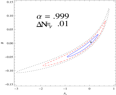
\subfigure[b]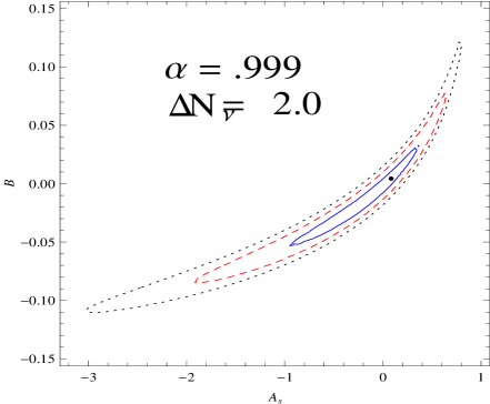
[a]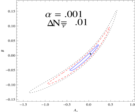
\subfigure[b]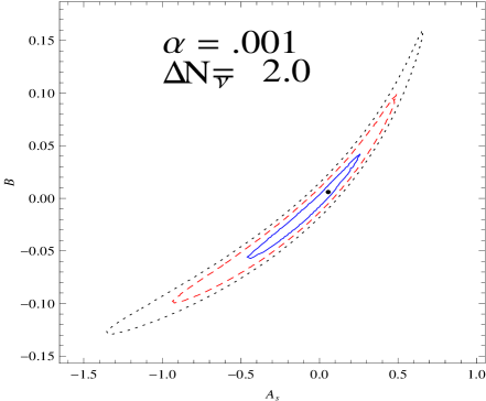
| Model | |||
|---|---|---|---|
| 0.003745 | 0.062817 | 0.232994 | |
| 0.016592 | 0.110548 | 0.099996 | |
| 0.006192 | 0.052076 | 0.807051 |
| Model | ||
|---|---|---|
| , | 0.00374357 | 0.0593243 |
| , | 0.00434955 | 0.0841938 |
| , | 0.00504535 | 0.0400150 |
| , | 0.00600186 | 0.0555941 |
The contours between and for closed universe for and are shown in figs. (1) and (2) respectively. Figures 1(a), 2(a) are drawn for =0.01 and Figures 1(b) and 2(b) are drawn for =2.0. From fig. 1(a) which is plotted for and =.01 for closed universe it appears that the value of lies in the range , , at , , confidence levels respectively. From fig. 1(b) which is plotted for and =2.0 for closed universe, the value of lies in the range , , at , , confidence levels respectively. It is evident from the analysis that the range of values of decreases with an increase of the effective neutrino parameter .
From fig. 2(a) which is plotted for and = 0.01 for closed universe, the value of lies in the range , , at , , confidence levels respectively. From fig. 2(b) which is plotted for and =2.0 for closed universe, the value of lies in the range , , at , , confidence levels respectively. It is clear from the above analysis that the range of values of increases with an increase in the effective neutrino parameter . Thus for a given vlaue of , the increase in neutrino parameter increases the range of parameter in the positive side.
[a]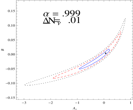
\subfigure[b]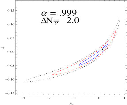
[a]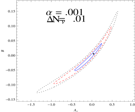
\subfigure[b]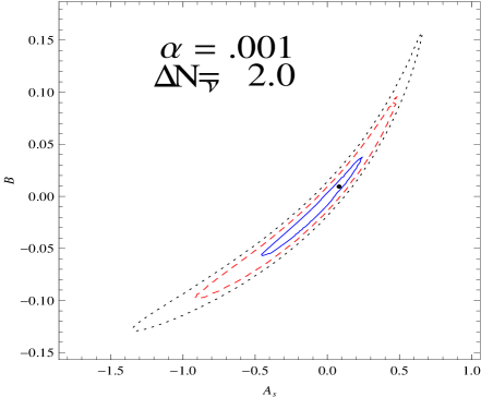
| Model | |||
|---|---|---|---|
| 0.007498 | 0.107866 | 0.100055 | |
| 0.010499 | 0.110576 | 0.100002 | |
| 0.016478 | 0.114298 | 0.100005 |
| Model | ||
|---|---|---|
| , | 0.00398596 | 0.0629336 |
| , | 0.00782675 | 0.133407 |
| , | 0.00528027 | 0.0418902 |
| , | 0.00937448 | 0.0817538 |
The contours between and for open universe for and are drawn in figs. (3) and (4) respectively. Figures 3 (a) and 4 (a) are drawn for =0.01 and Figures 3 (b) and 4(b) are drawn for =2.0. It is evident from fig. 3(a) which is plotted for and = 0.01 for open universe, that the parameter satisfies the following inequalities , , at , , confidence level respectively. In the fig. 3 (b), the allowed range of values of the parameter for and =2.0 for open universe are obtained which are given by , , at , , confidence levels respectively. It is evident that the domain of decreases with an increase of the effective neutrino parameter .
Figure 4(a) is plotted for and =.01 for open universe. In this case lies in the following ranges , , at , , confidence levels respectively. From fig. 4(b) which is plotted for and =2.0 for open universe, one can obtain viable cosmologies where satisfies the following inequalities , , at , , confidence levels respectively. It is evident from the contours drawn in fig. (4) that the range of increases with an increase in the effective neutrino parameter . But the positive range of values of decreases.
6 Numerical Analysis to determine constraints on the EOS parameters in beyond-detailed balance scenario
In this section we use data to constrain the parameters of the MCG that were used in detailed balance scenario of the previous section. Stern data set for () data has been used along with BAO peak parameter and CMB shift parameter. Chi-square minimisation technique has been used to determine the limiting values of the EOS parameters in the next subsections.
6.1 (H-z) data as a tool for constraining
The best-fitted parameters of the model considered here can be obtained by minimising the entity chi-square which is defined as
| (56) | |||
| (57) |
where is the observed Hubble parameter at redshift () and is the associated error with that particular observation. Hubble parameter is given by
| (58) |
where we denote
| (60) |
with
| (61) |
In this case data is taken from Stern Data analysis (Stern et. al., 2010). There are 12 data points of at redshift used to constrain the MCG model.
6.2 BAO peak parameter as a tool for constraining
A model independent BAO (Baryon Acoustic Oscillation) peak parameter can be defined for low redshift () measurements as:
| (62) |
where is the matter density parameter for the Universe. For a detailed description of the above defined parameter and related approximations reader is referred to (Eisenstein et. al., 2005). The chi-square function can be defined as usual:
| (63) |
where we have used the measured value for () as obtained by (Eisenstein et. al., 2005) from the SDSS data for LRG (Luminous Red Galaxies) survey.
6.3 CMB Shift Parameter as a tool for constraining
Here the CMB shift parameter is defined as
| (64) |
where is the z at last scattering. The WMAP7 data gives us at (Komatsu et. al., 2010). Chi square is defined as
| (65) |
6.4 Joint Analysis with (H-z) +BAO+CMB
We define total chi-square function for our joint analysis as:
| (66) |
The statistical analysis with gives the bounds on the model parameter specially on .
[b]![[Uncaptioned image]](/html/1205.2796/assets/x9.png) \subfigure[c]
\subfigure[c]![[Uncaptioned image]](/html/1205.2796/assets/x10.png)
Fig. 5(a) is plotted for with best-fitted values of , and . The parameter satisfies the following inequalities , , at , , confidence levels respectively. Fig. 5(b) is plotted for for best-fitted values of , and . The parameter in this case satisfies the folowing inequalities: , , at , , confidence levels respectively. Fig. 5(c) is plotted for for best-fitted value of , and . We note that the parameter satisfies the following inequalities , , at , , confidence levels respectively. It is evident that the allowed range of values of the parameter becomes larger compared to that of the detailed balance scenario (Paul et. al., 2012).
[b]![[Uncaptioned image]](/html/1205.2796/assets/x11.png)
Fig. 6(a) is plotted for and =0.01 for best-fitted value of and , it is evident that can take any value in the following ranges , , at , , confidence levels respectively. Fig. 6(b) is plotted for and =2.0, it is evident that the value of B lies in the range , , at , , confidence levels respectively. The figs. 6(a)- 6(b) show that the range of permissible values of decreases with an increase in the effective neutrino parameter.
[b]![[Uncaptioned image]](/html/1205.2796/assets/x12.png)
Fig. 7(a) is plotted for and =0.01 for best-fitted value of and , it is evident that the permissible values of now lies in the range , , at , , confidence levels respectively. Fig. 7(b) is plotted for and =2.0, it is evident that the values of lies in the range , , at , , confidence levels respectively. The contours drawn in figs 7(a) and 7(b) show that the range of permissible values of now decreases with an increase in the effective neutrino parameter. We note that the allowed range of values of the parameter , decreased appreciably here compared to that obtained from figs. 5 (a)-5 (c). This signifies the fact that as the contribution of dark radiation increases (through effective neutrino parameter) the range of admissible values of decreases in the case of beyond detailed-balance scenario which is same as one obtains in the case of detailed balance scenario.
7 Viability of MCG in HL gravity
In this section we discuss some of the implications of the present scenario. Here we determine the evolution of the equation of state parameter of the total cosmic fluid of the universe which is defined as , with the total pressure and energy density in the case of detailed-balance scenario. The pressure and energy density are given by
| (67) |
| (68) |
In the case of beyond-detailed balance scenario the total pressure and the energy density is given respectively as
| (69) | |||||
| (70) |
Here we replace the scale factor by redshift parameter, and the expression for density parameter and the Hubble parameter are expressed in terms of the redshift parameter in the equation of state. Consequently we get
| (71) |
. From the plot of with , for beyond detailed-balance scenario we note that at high redshift (i.e., early times) it attains a fixed value since radiation dominates in that epoch. In the intermediate redshift it behaves as dust for quite a long time. It is observed that the equation of state parameter picks up negative values at small redshift, i.e., at very recent past. In the case of closed or open universe the present value of the equastion of state parameter is found to be negative (-0.7) which admits a late accelerating universe.
In order to check the validity of the scenario we employed the best-fit values of the parameters of the MCG to find supernovae magnitudes () at different redshift and plotted vs. curve. We compared these with original curves of Union2 data and observed an excellent agreement.
8 Discussion
In this paper we present cosmologies with modified Chaplygin gas (MCG) in HL gravity scenario taking into account detailed balance and beyond detailed balance conditions both in the presence and absence of dark radiation. The equation of state of MCG has three unknown parameters. The permissible values of these parameters are explored from the observed data. Using data from different observations, namely, (OHD), BAO peak, CMB shift parameter data, we determine the admissible values of the EOS parameters considered here. In the MCG we have a parameter that represents the matter part. We analyze and determine the allowed range of values of for viable cosmologies. The analysis is carried out here both in the case of open and closed universe at , , confidence levels.
In a close universe we note that the permissible values of parameter lies in the range , , at , , confidence levels respectively for a maximum value of effective neutrino parameter. The range of obtained here is less than that obtained for best-fit value of effective neutrino parameter when dark radiation is not taken into account (Paul et. al., 2012).
It is evident from the figures 2 (a) and 2(b) that the range of increases with an increase in the effective neutrino parameter . In an open universe, the parameter lies in the range , , at , , confidence levels respectively for maximum value of effective neutrino parameter. The domain of is found to be less than that obtained for best-fit value of effective neutrino parameter without dark radiation (Paul et. al., 2012).
It appears from the analysis of a close and an open universe that in a close universe the domain of admissible values is comparatively narrower than that of an open universe at , , confidence levels respectively. We alaso note that the may take negative values in this case. The negative value of implies existence of exotic matter. In the literatures (Fabris et. al., 2010) the acceptable value of as was predicted to be very small, which once again gets support from our analysis.
In the beyond-detailed balance scenario there are six free parameters, namely , , , , , . It is found that the entire range of effective neutrino parameter is consistent with observations from our numerical analysis. The dependence of the extreme values of the neutrino parameter on other parameters are also shown in figs. (6) and (7).
The contours drawn in fig. (5) for beyond-detailed balance with different for best-fitted value of , and projects the admissible values of which lies in the range , , at , , confidence levels respectively. Thus the range of in this case become larger than that of detailed balance scenario without dark radiation (Paul et. al., 2012).
The contours drawn in fig. 6(a) which is plotted for and =0.01 for best-fitted value of and , projects the admissible values of which lies in the range , , at , , confidence levels respectively. The contours drawn in fig. 6(b) which is plotted for and =2.0, permits the values of the parameter which lies in the range , , at , , confidence levels respectively. It is clear that the range of values of decreases with an increase of the effective neutrino parameter.
The contours drawn in fig. 7(a) which is plotted for and =0.01 for best-fitted value of and gives the allowed values of which lies in the range , , at , , confidence levels respectively. The contours drawn in fig. 7(b) which is plotted for and =2.0 gives the allowed values of which lies in the range , , at , , confidence levels respectively. It is clearly visible from above analysis that the range of values of decreases with an increase in effective neutrino parameter.
We note that the range of values of decreases appreciably here compared to that obtained from the figs. 5 (a)- 5 (c). This signifies that as the contribution of dark radiation increases (through effective neutrino parameter) the contribution to the permissible range of values of decreases in beyond detailed-balance scenario like that one obtains in the case of detailed balance scenario (Paul et. al., 2012). In figure (8) we plot the variation of the total equation of state parameter with redshift parameter for beyond detailed-balance scenario. The curve shows the evolutionary phases of the universe efficiently. It is evident that at high redshift (early times) the of equation of state parameter attains , indicating radiation domination in that epoch. However, in the intermediate redshift we note that dust dominates through MCG for quite a long period of time. The best fit values of , and are shown in tables (1) and (2) for close universe and tables (3) and (4) are shown for open universe.
Using the best-fit values in beyond-detailed balance scenario vs redshift curve is plotted in fig. (9) and the figure is compared with Union Compilation data. It is evident from the figure that cosmologies in Horava-Lifshitz gravity with MCG fits well with the experimental result.
In this analysis we studied the dependance of extreme values of on other parameters in detailed balance scenario with MCG. We also present here results obtained on the beyond-detailed balance scenario. In the case of beyond-detailed balance scenario (BDB) there are two more free parameters and found that the theory is rich and all the features of cosmologies can be accommodated with MCG. Earlier in the Einstein-frame, MCG is employed to obtain viable cosmological models (Thakur, Ghose & Paul, 2009; Jianbo et al., 2010). Here MCG is employed in the HL gravity and determined various physical parameters of the universe which gets supports from observations. However, the present analysis does not enlighten the conceptual issues in HL gravity. It is important to look into details why the neutrino parameter is very small in HL gravity with MCG which will be discussed elsewhere.
9 Acknowledgements
The authors would like to thank IUCAA Reference Centre at North Bengal University for extending necessary research facilities to initiate the work. BCP would like to thank Inter-University Centre for Astronomy Astrphysics (IUCAA), Pune for hospitality to complete the work.
References
- Penzias, Wilson (1965) Penzias A. A. and Wilson R. W., 1965, Astrophys. J. Lett., 142, 419
- Dicke et al. (1965) Dicke R. H., Peebles P.J. E., Roll P.J. and Wilkinson, D. T., (1965), Astrophys. J. Lett., 142, 414
- Guth (1981) Guth A. H., 1981, Phys. Rev. D 23, 347
- Linde (1982) Linde A., 1982, Phys. Lett D 108, 389
- Albrecht & Steinhardt (1982) Albrecht A. and Steinhardt P., 1982, Phys. Rev. Lett. 48, 1220
- Sato (1981) Sato K., 1981, Mon. Not. Roy. Astron. Soc., 195, 467
- Riess et al. (1998) Riess A. G., et al., 1998, Astron J., 116, 1009
- Bojowald (2001) Bojowald M., 2001, Phys. Rev. Lett. 86, 5227
- Horava (2009) Horava P., 2009, JHEP 0903, 020 (2009) [arXiv: 0812.4287].
- Lu, Mei & Pope (2009) Lu H., Mei J. and Pope C. N., 2009, Phys. Rev. Lett. 103, 091301 [arXiv: 0904.1595].
- Calcagni (2009) Calcagni G., 2009 JHEP 0909, 112 ; arXiv: 0904.0829.
- Kiritsis & Kofinas (2009) Kiritsis E. and Kofinas G., 2009, Nucl. Phys. B 821, 467; [arXiv:0904.1334 [hep-th]].
- Sotiriou, Visser & Weinfurtner (2009) Sotiriou T., Visser M. and Weinfurtner S., 2009 Phys. Rev. Lett. 102, 251601; [arXiv:0904.4464], 2009, JHEP 0910, 033; [arXiv:0905.2798].
- Sotiriou, Visser & Weinfurtner (2009) Sotiriou T., Visser M. and Weinfurtner S., 2009, JHEP 0910, 033; [arXiv:0905.2798 [hep-th]].
- Mukohyama et al. (2009) Mukohyama S., Nakayama K., Takahashi F. and Yokoyama S., 2009, Phys. Lett. B 679, 6; [arXiv:0905.0055 [hep-th]].
- Park (2009) Park M. I., 2009, preprint: [arXiv:0910.1917 [hep-th]].
- Myung (2009) Myung Y. S., [arXiv:0911.0724 [hep-th]].
- Gao et. al. (2009) Gao X., Wang Y., Brandenberger R., Riotto A.,[arXiv:0905.3821 [hep-th]].
- Cai and Zhang (2009) Cai Y. F. and Zhang X., 2009 Phys. Rev. D 80, 043520; [arXiv:0906.3341 [astro-ph.CO]].
- Wang and Maartens (2010) Wang A. and Maartens R., 2010, Phys. Rev. D 81, 024009; [arXiv:0907.1748 [hep-th]].
- Danielsson and Thorlacius (2009) Danielsson U. H. and Thorlacius L., JHEP 0903, 070; [arXiv:0812.5088 [hep-th]].
- Cai, Cao & Ohta (2009) Cai R. G., Cao L. M. and Ohta N., 2009, Phys. Rev. D 80, 024003; [arXiv:0904.3670 [hep-th]].
- Kehagias & Sfetsos (2009) Kehagias A. and Sfetsos K., 2009, Phys. Lett. B 678, 123 (2009); [arXiv:0905.0477 [hep-th]].
- Park (2010) Park M. I., 2010, JCAP 1001, 001; [arXiv:0906.4275[hep-th]].
- Chaichian et. al. (2010) Chaichian M., Nojiri S., Odintsov S. D., Oksanen M. and Tureanu A., preprint : [arXiv:1001.4102 [hep-th]].
- Dutta & Saridakis (2010) Dutta S. and Saridakis E.N., 2010, JCAP 1001, 013; [arXiv:0911.1435 [hep-th]].
- Kim et. al. (2009) Kim S. S., Kim T. and Kim Y., 2009, Phys. Rev. D 80, 124002; [arXiv:0907.3093 [hep-th]].
- Harko (2009) Harko T., Kovacs T. and Lobo F. S., [arXiv:0908.2874[gr-qc]].
- Iorio and Ruggiero (2009) Iorio L. and Ruggiero M. L., 2009, preprint: [arXiv:0909.2562 [gr-qc]].
- Wang & Wu (2009) Wang A. and Wu Y., 2009, JCAP 0907, 012; [arXiv:0905.4117 [hep-th]].
- Cai, Cao & Ohta (2009) Cai R. G., Cao L.M. and Ohta N., 2009, [arXiv:0905.0751[hep-th]].
- Ali et. al. (2010) Ali A., Dutta S. and Saridakis E. N. and Sen A., 2010, preprint: [arXiv:1004.2474 [astro-ph.CO]].
- Billic, Tupper & Viollic (2001) Billic N., Tupper G. B., Viollic R. D., 2001, Phys. Lett. B, 535, 17.
- Bento, Bertolami & Sen (2002) Bento M. C., Bertolami O., Sen A. A., 2002, Phys. Rev. D, 66, 043507
- Chaplygin (1904) Chaplygin S., 1904, Sci. Mem. Moscow Univ. Math. Phys., 21 1
- Bazeia (1999) Bazeia D., 1999, Phys. Rev. D 59 085007
- Jackiw & Polychronakos (1999) Jackiw R., Polychronakos A. P. , 1999, Commun. Math. Phys. 207 107
- Bordemann & Hoppe (1993) Bordemann M. and Hoppe J., 1993, Phys. Lett. B 317 315
- Silva & Bertolami (2003) Silva P.T., Bertolami O., 2003 Ap. J,599, 829
- Dev & Alcaniz (2004) Dev A., Alcaniz J.S., 2004 A & A, 417, 847
- Bertolami & Silva (2006) Bertolami O., Silva P. T., 2006, Mon. Not, R. Astron. Soc., 365, 1149
- Liu & Lu (2005) Liu D. J., Li X. Z., 2005, preprint:[arxiv:0501115 [astro-ph]].
- Debnath, Banerjee and Chakraborty (2004) Debnath U., Banerjee A., Chakraborty S., 2004, preprint [arXiv:0411015 [gr-qc/]].
- Kowalaski et al. (2008) Kowalaski M., et al., 2008, preprint: [arXiv:0804.4142].
- Horava (2009) Horava P., Phys. Rev. D 79, 084008; [arXiv:0901.3775 [hep-th]].
- Carloni, Elizalde & Silva (2009) Carloni S., Elizalde E. and Silva P. T., 2009, preprint: [arXiv:0909.2219 [hep-th]].
- Thakur, Ghose & Paul (2009) Thakur P., Ghose S. and Paul B.C., 2009, Mon. Not. R. Astron. Soc. 397, 1935
- Jianbo et al. (2010) Jianbo L., Lixin X., Jiechao L., Baorong C., Yuanxing G. and Hongya L., 2010, preprint :[arXiv:1004.3361v1[astro.ph.co]].
- Hagiwara et. al. (2002) Hagiwara K., et. al., 2002, [Particle Data Group], Phys. Rev. D 66 , 010001
- Olive, Steigman & Walker (2000) Olive K. A., Steigman G. and Walker T. P., 2000, Phys. Rept. 333, 389; [arXiv:9905320 [astro-ph]].
- Steigman (2006) Steigman G., 2006, Int. J. Mod. Phys. E 15, 1; preprint: [arXiv:0511534 [astro-ph]].
- Komatsu et. al. (2010) Komatsu E., et al., 2010, preprint:[arXiv:1001.4538 [astro-ph.CO]].
- Eisenstein et. al. (2005) Eisenstein D. J., et al., 2005, Astrophys. J. 633, 560
- Stern et. al. (2010) Stern D., et al., 2010, JCAP 1002, 008
- Fabris et. al. (2010) Fabris J.C., Velten H. E. S., Ogouyandjou C. and Tossa J., 2010, preprint: [arXiv:1007.1011v1 [astro-ph.CO]].
- Ichikawa, Seekiguchi & Takahashi (2008) Ichikawa K., Seekiguchi T. and Takahashi T., 2008, preprint: arXiv: 0803.0889 [astro-ph] (2008).
- Paul et. al. (2012) Paul B. C., Thakur P. and Saha A., 2012 Phys. Rev.D 85, 024039
- Bogdanos & Sarikdakis (2010) Bogdanos C. and Sarikdakis E.N., 2010, Class.Quant.Grav. 27, 075005
- Malaney and Mathews (1993) Malaney R. A. and Mathews G.J., 1993, Phys. Rept. 209, 145
- Joyce (1997) Joyce M., 1997, Phys. Rev. D 55, 1875; preprint: [arXiv:hep-ph/9606223].
- Joyce and Prokopec (1998) Joyce M. and Prokopec T., 1998, Phys. Rev. D 57, 6022; preprint:[arXiv:hep-ph/9709320].
- Charmousis et. al. (2009) Charmousis C., Niz G., Padilla A. and Saffin P. M., 2009 JHEP 0908,070; preprint: [arXiv:0905.2579[hep-th]].
- Leon & Saridakis (2009) Leon G. and Saridakis E. N., 2009, JCAP 0911, 006; preprint: [arXiv:0909.3571[hep-th]].
- Clarkson, Cortes & Bassett (2007) Clarkson C., Cortes M. and Bassett B. A., 2007, JCAP 0708,011; preprint: [arXiv:astro-ph/0702670].
- Virey et. al. (2008) Virey J.M., Talon-Esmieu D., Ealet A., Taxil P. and Tilquin A., 2008JCAP 0812,008; preprint:[arXiv:0802.4407[astro-ph]].