Primordial Non-Gaussianity in the Forest: 3D Bispectrum of Ly-$\alpha$ Flux Spectra Along Multiple Lines of Sight

Abstract

We investigate the possibility of constraining primordial non-Gaussianity using the 3D bispectrum of Ly-$\alpha$ forest. The strength of the quadratic non-Gaussian correction to an otherwise Gaussian primordial gravitational field is assumed to be dictated by a single parameter $f_{{}_{\rm NL}}$. We present the first prediction for bounds on $f_{{}_{\rm NL}}$ using Ly-$\alpha$ flux spectra along multiple lines of sight. The 3D Ly-$\alpha$ transmitted flux field is modeled as a biased tracer of the underlying matter distribution sampled along 1D skewers corresponding to quasars sight lines. The precision to which $f_{{}_{\rm NL}}$ can be constrained depends on the survey volume, pixel noise and aliasing noise (arising from discrete sampling of the density field). We consider various combinations of these factors to predict bounds on $f_{{}_{\rm NL}}$. We find that in an idealized situation of full sky survey and negligible Poisson noise one may constrain $f_{{}_{\rm NL}}\sim 23$ in the equilateral limit. Assuming a Ly-$\alpha$ survey covering large parts of the sky ($k_{min}=8\times 10^{-4}{\rm Mpc}^{-1}$) and with a quasar density of ${\bar{n}}=5\times 10^{-3}\rm Mpc^{-2}$ it is possible to constrain $f_{{}_{\rm NL}}\sim 100$ for equilateral configurations. The possibility of measuring $f_{{}_{\rm NL}}$ at a precision comparable to LSS studies maybe useful for joint constraining of inflationary scenarios using different data sets.

Introduction: The widely popular paradigm of slow-roll inflation driven by a single canonical scalar field generates adiabatic perturbations which are largely Gaussian in nature and leads to a nearly scale invariant power spectrum  maldacena-2003 . Several theoretical predictions however point towards mild to severe departure from Gaussianity Bartolo et al. (2004). Measuring the degree of non-Gaussianity is hence crucial towards discriminating between various inflationary scenarios thereby enhancing our understanding of the very early Universe. It is assumed that on sub-horizon scales the primordial gravitational potential $\Phi^{\rm prim}$ is related to a Gaussian random field $\phi_{G}$ through a non linear relation of the form $\Phi^{\rm prim}=\phi_{G}+\frac{f_{{}_{\rm NL}}}{c^{2}}\left({\phi_{G}}^{2}-\langle{\phi_{G}}^{2}\rangle\right)$. Departures from Gaussianity may hence be quantified using the parameter $f_{{}_{\rm NL}}$. We assume that $f_{{}_{\rm NL}}$ is scale independent - a reasonable prediction for most inflationary models where non-Gaussianity is generated on super-horizon scales. The value of $f_{{}_{\rm NL}}$ obtained from slow-roll inflation turns out to be very small $({\cal O}~{}(10^{-3}-10^{-2}))$ maldacena-2003 . This implies that any detection of large $f_{{}_{\rm NL}}$ shall rule out all canonical single field slow-roll inflation models. The mean value of $f_{{}_{\rm NL}}$ ($26\pm 140$ for equilateral and $32\pm 21$ in local limit for $1\sigma$ CL) obtained from WMAP data wmap-7 seems to indicate large non-Gaussianity. Although low SNR in these results indicate that we are yet to detect the primordial non-Gaussianity, it is expected that data from the Planck satellite shall give a much tighter constraint on $f_{{}_{\rm NL}}$ and the error is expected to come down to $\Delta f_{{}_{\rm NL}}\sim\pm 5$ in the local limit. Other than CMBR observations, a measurement of the bispectrum or the three point correlation function of the galaxy distribution Desjacques and Seljak (2010) is a standard alternative method to constrain primordial non-Gaussianity. These probes however only provide weak bounds on $f_{{}_{\rm NL}}$ as compared to the CMBR observations (SDSS for example can measure $|f_{{}_{\rm NL}}|\sim 10^{3}-10^{4}$).

In the post reionization epoch, small fluctuations of the neutral hydrogen (HI) density field in a predominantly ionized IGM leads to a series of distinct absorption features - the Ly-$\alpha$ forest Rauch (1998) in the spectra of background quasars. The Ly-$\alpha$ forest is a well established powerful probe of cosmology Rauch (1998); psbs . Traditional Ly-$\alpha$ studies have considered the power spectrum or bispectrum of the one dimensional transmitted flux field psbs corresponding to the quasar line of sight. This approach is reasonable when the angular density of quasars on the sky is low. The new generation of quasar surveys (the ongoing BOSS and future BigBOSS) however promise to achieve a very high quasar density and cover large fractions of the sky. This has led to the possibility of measuring the 3D Ly-$\alpha$ power spectrum along multiple lines of sight multiplelos . We note that the first hydro simulation of the Ly-$\alpha$ forest in non-Gaussian scenarios is presented in an earlier work viel09 .

In this letter we investigate the possibility of constraining $f_{{}_{\rm NL}}$ using the 3D Ly-$\alpha$ forest bispectrum. Similar to the power spectrum studies, the Ly-$\alpha$ flux distribution is assumed to be a biased tracer of the underlying matter field sampled along discrete sight lines. We explore the range of observational parameters for the constraints on $f_{{}_{\rm NL}}$ from the 3D analysis to be competitive with CMBR and LSS (large scale structure) studies.

Formalism: The post-reionization matter density field $\Delta_{{\bf k}}$ in Fourier space is related to the primordial gravitational potential on sub-horizon scales as $\Delta_{{\bf k}}(z)={\cal{M}}(k,z)\Phi^{\rm prim}_{{\bf k}}$. The function ${\cal M}(k,z)$ is given by ${\cal{M}}(k,z)=-\frac{3}{5}\frac{k^{2}T(k)}{\Omega_{m}H_{0}^{2}}D_{+}(z)$, where $T(k)$ denotes the matter transfer function and $D_{+}(z)$ is the growing mode of density fluctuations. We have used the BBKS transfer function bbks and cosmological parameters hazra-2010 obtained from a MCMC analysis on the WMAP7 data-sets. The power spectrum and bispectrum of the density field are defined as $\langle\Delta_{{\bf k}_{1}}\Delta_{{\bf k}_{2}}\rangle=\delta_{D}({\bf k}_{1}+{\bf k}_{2})P(k_{1})$ and $\langle\Delta_{{\bf k}_{1}}\Delta_{{\bf k}_{2}}\Delta_{{\bf k}_{3}}\rangle=\delta_{D}({\bf k}_{1}+{\bf k}_{2}+{\bf k}_{3})B(k_{1},k_{2},k_{3})$. Clearly, the linear power spectrum of the density field is given by $P^{\rm L}(k)={\cal{M}}(k,z)^{2}P_{\Phi}^{\rm prim}$ where $P_{\Phi}^{\rm prim}$ denotes the primordial power spectrum of the gravitational potential such that $P_{\Phi}^{\rm prim}=P_{\phi{G}}+{\cal{O}}(f_{{}_{\rm NL}}^{2})$. The powerspectrum $P_{\phi{G}}$ of the Gaussian field $\phi_{G}$ shall be assumed to be featureless and scale invariant. We note that a wide class of inflation models, including the simplest one comprising of a single inflaton field in a quadratic potential, introduces perturbations that are almost Gaussian and exhibit a power spectrum that is nearly scale invariant. It follows that in the realm of linear perturbation theory the bispectrum of the matter field arising from primordial non-Gaussianity is given by ${B^{\rm L}}_{123}={\cal{M}}(k_{1}){\cal{M}}(k_{2}){\cal{M}}(k_{3}){B_{\phi G}}_{123}$ where we use the notation ${123}\equiv(k_{1},k_{2},k_{3})$ and $B_{\phi G}$ is given by

$${B_{\phi G}}_{123}=\frac{2f_{{}_{\rm NL}}}{c^{2}}\left[P_{\phi G}(k_{1})P_{\phi G}(k_{2})+\rm{cyc}\right]+{\cal{O}}(f_{{}_{\rm NL}}^{3}).$$ (1)

Apart from the contribution to the bispectrum from primordial fluctuations, non-linear structure formation caused by gravitational instability leads to mode coupling and thereby induce additional non-Gaussianity. This is especially relevant when we use low redshift tracers to implicitly measure $n-$point functions of the matter density field. Using the second order perturbation theory the additional contribution to the matter bispectrum is

$$B^{\rm NL}_{123}=2F_{2}({\bf k}_{1},{\bf k}_{2})P(k_{1})P(k_{2})+\rm{cyc}.$$ (2)

where the second order correction is obtained from perturbation theory and we have adopted the form of $F_{2}$ from Desjacques and Seljak (2010). Finally, the total matter bispectrum is a sum of the contributions to non-Gaussianity arising from the intrinsic primordial fluctuations and that generated by non-linear evolution of an otherwise Gaussian field. Thus we have $B_{123}=B^{\rm L}_{123}+B^{\rm NL}_{123}$, where we have ignored the possible contribution from the primordial trispectrum. We use $B_{123}$ to obtain the 3D bispectrum of the Ly-$\alpha$ forest.

The Ly-$\alpha$ forest spectra are associated with gas distribution in voids or slightly overdense regions. Noting that the astrophysical structures associated with the spectra are only mildly non-linear, the transmitted flux $\mathcal{F}$ through the Ly-$\alpha$ forest may be modeled by assuming that the gas traces the underlying dark matter distribution psbs except on small scales where pressure plays an important role. Further, it is believed that photo-ionization equilibrium that maintains the neutral fraction also leads to a power law temperature-density relation tempdens . The fluctuating Gunn-Peterson approximation (FGPA)fgpa incorporates these assumptions to relate the transmitted flux $\mathcal{F}$ to the dark matter overdensity $\delta$ as ${\mathcal{F}}={\bar{\mathcal{F}}}~{}{\rm exp}\left[-A(1+\delta)^{2-0.7(\gamma-1)}\right]$, where ${\bar{\mathcal{F}}}$ is the mean transmitted flux and $(\gamma-1)$ is the slope of the temperature-density relation tempdens . We note that $\gamma$ imprints the reionization history of the Universe. The redshift dependent quantity $A$ Kim et al. (2007) depends on a number of parameters, like the IGM temperature, photo-ionization rate and cosmological parameters psbs . On large scales it is reasonable to believe that the fluctuations in the transmitted flux $\delta_{\mathcal{F}}=\left(\mathcal{F}/\bar{\mathcal{F}}-1\right)$ may be expanded as $\delta_{\mathcal{F}}=b_{1}\delta+\frac{1}{2}b_{2}\delta^{2}$ where, it is assumed that the Ly-$\alpha$ forest spectrum has been smoothed over some suitably large length scale. This relation allows analytic computation of statistical properties of $\delta_{\mathcal{F}}$. We note that corrections to this on small scales come from peculiar velocities, an effect we have not incorporated in our analysis for simplicity. At our fiducial redshift $z=2.5$, we adopt an approximate $(\bar{\mathcal{F}},\gamma,A)\equiv(0.8,\,1.5,\,0.16)$ from the numerical simulations of Ly-$\alpha$ forest McDonald (2003) and theoretical predictions Seljak (2012). We note however that these numbers are largely uncertain owing to inadequate modeling of the IGM. The bias, $b_{1}$ for example has a sensitive redshift dependence and may depend on the smoothing scale of the Ly-$\alpha$ spectra. Using the local bias model, the power spectrum $P_{\mathcal{F}}(k)$ and bispectrum ${\cal{B}}_{\mathcal{F}}$ of Ly-$\alpha$ forest flux fluctuations $\delta_{\mathcal{F}}$ are given by

$$P_{\mathcal{F}}(k) = b_{1}^{2}P(k)$$

$${\cal B}_{\mathcal{F}123} = b_{1}^{3}B_{123}+b_{1}^{2}b_{2}\left[P(k_{1})P(k_{2})+\rm{cyc}.\right]$$ (3)

The bispectrum of Ly-$\alpha$ flux is hence completely modeled using three parameters $(f_{{}_{\rm NL}},b_{1},b_{2})$. We shall now set up the Fisher matrix for constraining $f_{{}_{\rm NL}}$ using the Ly-$\alpha$ bispectrum. Following the formulation described in Desjacques and Seljak (2010) we define the bispectrum estimator as

$$\hat{{\cal B}}_{\mathcal{F}123}=\frac{V_{f}}{V_{123}}\int_{k_{1}}d^{3}{\bf q}_{1}\int_{k_{2}}d^{3}{\bf q}_{2}\int_{k_{3}}d^{3}{\bf q}_{3}\delta_{D}({\bf q}_{123})$$

$$\times~{}\Delta_{\mathcal{F}}^{o}(k_{1})\Delta_{\mathcal{F}}^{o}(k_{2})\Delta_{\mathcal{F}}^{o}(k_{3})$$ (4)

Here ${\bf q}_{123}={\bf q}_{1}+{\bf q}_{2}+{\bf{q}}_{3}$, ${V_{f}}=(2\pi)^{3}/V$ where $V$ is the survey volume, $V_{123}=\int_{k_{1}}d^{3}{\bf q}_{1}\int_{k_{2}}d^{3}{\bf q}_{2}\int_{k_{3}}d^{3}{\bf q}_{3}\delta_{D}({\bf q}_{123})$ and the integrals are performed over the $q_{i}-$ intervals $\left(k_{i}-\frac{\delta k}{2},k_{i}+\frac{\delta k}{2}\right)$. The quantities $\Delta_{\mathcal{F}}^{o}(k_{i})$ denotes the ‘observed’ Ly-$\alpha$ flux fluctuations in Fourier space. The observed quantity $\delta_{{\mathcal{F}}}^{o}({\bf{r}})$ is given by the continuous field $\delta_{{\mathcal{F}}}({\bf r})$ sampled along skewers corresponding to line of sight to bright quasars. We therefore have $\delta_{{\mathcal{F}}}^{o}({\bf{r}})=\delta_{{\mathcal{F}}}({\bf{r}})\times\rho({\bf{r}})$, where the sampling window function $\rho({\bf{r}})$ is defined as $\rho({\bf{r}})={\cal{N}}\frac{\sum_{a}w_{a}\ \delta_{D}^{2}({\bf{r}}_{\perp}-{\bf{r}}_{\perp a})}{\sum_{a}w_{a}}$, where ${\cal{N}}$ is a normalization such that $\int dV\rho({\bf{r}})=1$. The summation extends up to $N_{Q}$, the total number of quasar skewers in the field which are assumed to be distributed with sky locations ${\bf{r}}_{\perp a}$ . The weights $w_{a}$ introduced in $\rho({\bf{r}})$ are in general related to the pixel noise and can be chosen with a posteriori criterion of minimizing the variance. In Fourier space, we then have ${\Delta}_{{\mathcal{F}}}^{o}({\bf{k}})=\tilde{\rho}({\bf{k}})\otimes{\Delta_{\mathcal{F}}}({\bf{k}})+\Delta_{\mathcal{F}\rm noise}({\bf{k}})$, where $\tilde{\rho}$ is the Fourier transform of $\rho$, and $\Delta_{\mathcal{F}\rm noise}({\bf{k}})$ denotes a possible noise term.

If the bispectrum covariance matrix is diagonal which implies that no correlation exists between different triangle shapes, the simple variance of the estimator $\hat{{\cal B}_{\mathcal{F}}}$ can be calculated as $\Delta\hat{{\cal B}_{\mathcal{F}}}^{2}=\langle\hat{{\cal B}_{\mathcal{F}}}^{2}\rangle-\langle\hat{{\cal B}_{\mathcal{F}}}\rangle^{2}$. This is given at the lowest order by

$$\Delta\hat{{\cal B}_{\mathcal{F}}}^{2}=\frac{V_{f}}{V_{123}}sP_{\mathcal{F}}^{\rm Tot}(k_{1})P_{\mathcal{F}}^{\rm Tot}(k_{2})P_{\mathcal{F}}^{\rm Tot}(k_{3})$$ (5)

where $s=6,1$ for equilateral and scalene triangles respectively and $P_{\mathcal{F}}^{\rm Tot}(k)$ is the total power spectrum of Ly-$\alpha$ flux given by

$$P_{\mathcal{F}}^{\rm Tot}({\bf k})=P_{\mathcal{F}}({\bf k})+P^{\rm{1D}}_{\mathcal{F}}(k_{\parallel})P_{W}+N_{\mathcal{F}}$$ (6)

The quantity $P^{\rm 1D}_{\mathcal{F}}(k_{\parallel})$ is the usual 1D flux power spectrum psbs corresponding to individual spectra given by $P^{\rm{1D}}_{\mathcal{F}}(k_{\parallel})=(2\pi)^{-2}\int d^{2}{\bf k}_{\perp}P_{\mathcal{F}}({\bf k})$ and $P_{W}$ denotes the power spectrum of the window function. The quantity $N_{\mathcal{F}}$ denotes the effective noise power spectra for the Ly-$\alpha$ observations. The term $P^{\rm{1D}}_{\mathcal{F}}(k_{\parallel})P_{W}$ referred to as the ‘aliasing’ term, is similar to the shot noise in galaxy surveys and quantifies the discreteness of the 1D Ly-$\alpha$ skewers. It has been shown that an uniform weighing scheme suffices when most of the spectra are measured with a sufficiently high SNR multiplelos . This gives $P_{W}=\frac{1}{\bar{n}}$, where $\bar{n}$ is the 2D density of quasars ($\bar{n}=N_{Q}/{\mathcal{A}}$, where ${\mathcal{A}}$ is the area of the observed field of view). We assume that the variance $\sigma^{2}_{{\mathcal{F}}N}$ of the pixel noise contribution to $\delta_{\mathcal{F}}$ is the same across all the quasar spectra whereby we have $N_{\mathcal{F}}=\sigma^{2}_{\mathcal{F}N}/\bar{n}$ for its noise power spectrum. In arriving at equation (6) we have ignored the effect of quasar clustering. In reality, the distribution of quasars is expected to exhibit clustering Myers et al. (2007). However, for the quasar surveys under consideration, the Poisson noise dominates over the clustering and the latter may be ignored.

The Fisher matrix for a set of parameters $p_{i}$ is constructed as

$$F_{ij}=\sum_{k_{1}=k_{min}}^{k_{max}}\sum_{k_{2}=k_{min}}^{k_{1}}\sum_{k_{3}=\tilde{k}_{min}}^{k_{2}}\frac{1}{\Delta\hat{{\cal B}_{\mathcal{F}}}^{2}}\frac{\partial{{\cal B}_{\mathcal{F}123}}}{\partial p_{i}}\frac{\partial{{\cal B}_{\mathcal{F}123}}}{\partial p_{j}}$$ (7)

where $\tilde{k}_{min}=max(k_{min},|k_{1}-k_{2}|)$ and the summations are performed using $\delta k=k_{min}$. Assuming the likelihood function for $p_{i}$ to be a Gaussian the errors in $p_{i}$ is given by the Cramer-Rao bound $\sigma_{i}^{2}=F^{-1}_{ii}$. We have used this to investigate the power of a Ly-$\alpha$ survey to constrain $f_{{}_{\rm NL}}$.

Results: We consider quasars in the range $z=2$ to $3$ since the peak in redshift distribution of quasars occur in this range sneider . We note that for a given quasar at redshift $z=z_{Q}$, the proximity effect will not allow the spectrum to be measured in the region $10,000\,{\rm km\,s^{-1}}$ blue-wards of the Ly-$\alpha$ emission and only the region which is at least 1,000 $\rm km\,s^{-1}$ red-ward of the quasar’s Ly-$\beta$ and O-$\rm VI$ lines are considered to avoid the possible confusion with these lines. We have chosen $z=2.5$ as out fiducial redshift for the subsequent analysis. We note here that all the parameters involved in the modeling the Ly-$\alpha$ forest, have direct or indirect redshift dependence.

A Ly-$\alpha$ forest survey towards measurement of power spectrum or bispectrum is characterized by the survey volume, pixel noise in the spectra and the number density of the quasar skewers. The constraining power of the survey shall depend directly on the choice of these parameters. In the cosmic variance limit the minimum $f_{{}_{\rm NL}}$ that can be measured depends on the number of Fourier modes in the survey volume V given by $N_{k}=4\pi/3k_{max}^{2}V/(2\pi)^{3}$. Clearly the minimum detectable $f_{{}_{\rm NL}}$ is a function of $k_{max}$ and $k_{min}$. The noise power spectrum $N_{\mathcal{F}}$ is given by $N_{\mathcal{F}}={\bar{\mathcal{F}}}^{\,-2}[S/N]^{-2}_{\Delta x}(\Delta x/1{\rm Mpc})$ where $[S/N]_{\Delta x}$ is the signal to noise ratio for a spectrum smoothed to a resolution $\Delta x$. We quote $[S/N]$ here for $1~{}\mathring{A}$ pixels. The main source of noise to the 3D power spectrum comes from the aliasing noise term and one requires a very high density of quasars in the field of view for this term to be sub-dominant.

Figure 1: The $68.3\%$, $95.4\%$ and $99.8\%$ likelihood confidence contours for the parameters $(f_{{}_{\rm NL}},b_{1})$. Shown in the figure are the values $(k_{min},{\bar{n}},S/N)$ used to compute the Fisher matrix.

$k_{min}$	${\bar{n}}$	$S/N$	$\Delta f_{{}_{\rm NL}}$	$\Delta b_{1}$
(${\rm Mpc^{-1}}$)	(${\rm Mpc^{-2}}$)
$2\times 10^{-3}~{}~{}~{}~{}$	$~{}~{}~{}~{}2.2\times 10^{-3}~{}~{}~{}~{}$	$5$	$~{}~{}~{}~{}228.84~{}~{}$	$~{}~{}~{}~{}1.1\times 10^{-2}$
$1\times 10^{-3}~{}~{}~{}~{}$	$~{}~{}~{}~{}2.2\times 10^{-3}~{}~{}~{}~{}$	$5$	$~{}~{}~{}~{}161.81~{}~{}$	$~{}~{}~{}~{}7.7\times 10^{-3}$
$5\times 10^{-4}~{}~{}~{}~{}$	$~{}~{}~{}~{}2.2\times 10^{-3}~{}~{}~{}~{}$	$5$	$~{}~{}~{}~{}114.42~{}~{}$	$~{}~{}~{}~{}5.5\times 10^{-3}$
$8\times 10^{-4}~{}~{}~{}~{}$	$~{}~{}~{}~{}1.0\times 10^{-3}~{}~{}~{}~{}$	$5$	$~{}~{}~{}~{}272.95~{}~{}$	$~{}~{}~{}~{}1.5\times 10^{-2}$
$8\times 10^{-4}~{}~{}~{}~{}$	$~{}~{}~{}~{}2.2\times 10^{-3}~{}~{}~{}~{}$	$5$	$~{}~{}~{}~{}144.73~{}~{}$	$~{}~{}~{}~{}6.9\times 10^{-3}$
$8\times 10^{-4}~{}~{}~{}~{}$	$~{}~{}~{}~{}5.0\times 10^{-3}~{}~{}~{}~{}$	$5$	$~{}~{}~{}~{}91.65~{}~{}$	$~{}~{}~{}~{}3.5\times 10^{-3}$
$8\times 10^{-4}~{}~{}~{}~{}$	$~{}~{}~{}~{}2.2\times 10^{-3}~{}~{}~{}~{}$	$2$	$~{}~{}~{}~{}263.52~{}~{}$	$~{}~{}~{}~{}1.5\times 10^{-2}$
$8\times 10^{-4}~{}~{}~{}~{}$	$~{}~{}~{}~{}2.2\times 10^{-3}~{}~{}~{}~{}$	$3$	$~{}~{}~{}~{}182.83~{}~{}$	$~{}~{}~{}~{}9.5\times 10^{-3}$
$8\times 10^{-4}~{}~{}~{}~{}$	$~{}~{}~{}~{}2.2\times 10^{-3}~{}~{}~{}~{}$	$4$	$~{}~{}~{}~{}156.56~{}~{}$	$~{}~{}~{}~{}7.7\times 10^{-3}$
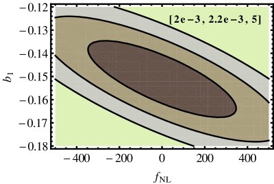
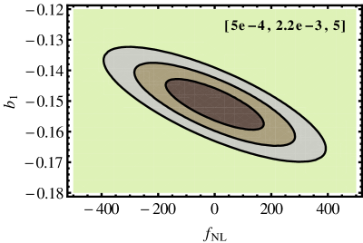
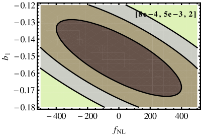
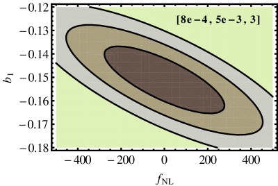
Ideal case
$5\times 10^{-4}~{}~{}~{}~{}$	$~{}~{}~{}~{}1~{}~{}~{}~{}$	$5$	$~{}~{}~{}~{}23.72$	$~{}~{}~{}~{}2.1\times 10^{-4}$

Table 1: The bounds on ($f_{{}_{\rm NL}},~{}b_{1}$) obtained from Fisher analysis for various combinations of ($k_{min},~{}{\bar{n}},~{}S/N$).

The bispectrum SNR depends on the triangle configurations considered to evaluate it. In this work we have used the simplest equilateral configurations characterized by just a single Fourier mode. This over estimates the noise by at least a factor of $\sim 2.45$ as compared to the case with arbitrary triangles. In the equilateral limit the 3D Ly-$\alpha$ bispectrum can be written as ${\cal B}_{\mathcal{F}}(k)=P(k)^{2}\left[\frac{a_{1}}{{\cal M}(k)}+a_{2}\right]$ where $a_{1}=6b_{1}^{3}f_{{}_{\rm NL}}/c^{2}$ and $a_{2}=6b_{1}^{3}F_{2}+3b_{1}^{2}b_{2}$. Only two parameters are sufficient to model the bispectrum instead of three parameters $(f_{{}_{\rm NL}},b_{1},b_{2})$ for the general case. We use the fiducial values $(f_{{}_{\rm NL}},b_{1},b_{2})\equiv(0,-0.15,-0.075)$ and choose $f_{{}_{\rm NL}}$ and $b_{1}$ to be the free parameters for the Fisher analysis. We recall that in our modeling of the Ly-$\alpha$ forest we used the parameters (${\bar{\mathcal{F}}},A,\gamma$). The parameter $\bar{\mathcal{F}}$ does not appear in $\delta_{\mathcal{F}}$ and there is degeneracy between the parameters $A$ and $\gamma$ which only appears as a product in $b_{1}$. Changing $b_{1}$ hence amounts to changing either or both $A$ and $\gamma$.

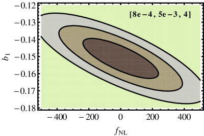
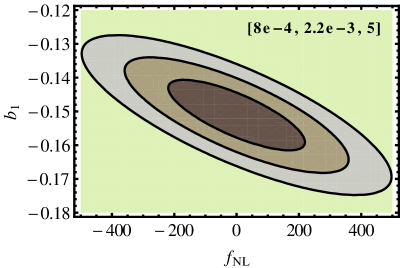
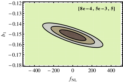
We assume that the likelihood function is a bivariate Gaussian which yields the confidence ellipses shown in figure (1). The tilt of the error ellipses indicate correlation between the parameters. We quantify this using the correlation coefficient $r=F^{-1}_{12}/\sqrt{F^{-1}_{11}F^{-1}_{22}}$. For the range of parameters chosen we find that this is roughly constant $r\sim-0.7$.

In the ideal situation of full sky coverage and negligible Poisson noise we find that $\Delta f_{{}_{\rm NL}}\sim 23$ in the equilateral limit. We tabulate our results for varying sky coverage ($k_{min}^{-3}=V/(2\pi)^{3}$), Poisson noise ($\sim 1/{\bar{n}}$) and pixel noise ($S/N$) in Table 1. As expected we have tighter constraints on ($f_{{}_{\rm NL}},b_{1}$) with increasing survey volume, ${\bar{n}}$ and $S/N$. The values of the survey parameters chosen are reasonable and achievable by future Ly-$\alpha$ surveys. Exploiting the entire sky coverage of SDSS we find that one can obtain a bound on $f_{{}_{\rm NL}}\sim 100$ (in equilateral configuration) for a survey with ${\bar{n}}=5\times 10^{-3}~{}{\rm Mpc}^{-2}$ when the spectra are measured at $5\sigma$ level.

Our analysis has largely focussed on the equilateral configuration. However we find that the Cramer-Rao bound for $f_{NL}$ in the squeezed limit ($k_{3}<<min(k_{1},k_{2})$) turns out to be $\sim 40-100$ for the cases we have considered. The case of arbitrary triangular configuration is to be addressed in our future work  sarkar-prep . However, our preliminary estimates show us that we may constrain $f_{NL}\sim 1$ in an ideal environment. For example using $S/N\sim 5$, $\bar{n}\sim 10^{-3}\rm Mpc^{-3}$ and $k_{min}\sim 10^{-3}\rm Mpc^{-1}$, we have $\Delta f_{NL}\sim 5$ in the case of arbitrary triangles, which is competitive with CMBR and LSS studies.

Our discussion so far has bypassed the issue of redshift space distortion arising from peculiar motion. The bispectrum in redshift space shall depend not only on the shape of the triangle but also on its orientation with the line of sight. This shall introduce two more angular parameters in the analysis. The multipole expansion of bispectrum in redshift space provides a way to break the degeneracy between bias and cosmological growth parameter $f\sim\Omega_{m}^{0.6}$. We plan to take this up in a future work sarkar-prep . However the spherically averaged bispectrum is related to its real space counterpart as ${\mathcal{B}}_{\mathcal{F}}^{s}=\left(1+\frac{2}{3}\beta+\frac{1}{9}\beta^{2}\right){\mathcal{B}}_{\mathcal{F}}$ where $\beta=f/b_{1}$ sefu . This is an enhancement on all scales.

To conclude, we emphasize that it is possible to put stringent bounds on primordial non-Gaussianity from the measured 3D bispectrum of the Ly-$\alpha$ forest along multiple lines of sight and thereby constrain various inflationary scenarios. Our analytic predictions indicate that such studies with future Ly-$\alpha$ surveys may be useful while performing a joint analysis using other data sets like CMBR or LSS.

References

- (1) J. Maldacena, JHEP 0305, 013 (2003); D. K. Hazra, L. Sriramkumar and J. Martin, arXiv:1201.0926v1 [astro-ph.CO]
- Bartolo et al. (2004) N. Bartolo, E. Komatsu, S. Matarrese, and A. Riotto, Phys. Rep., 402, 103 (2004)
- (3) D. Larson et al., Astrophys. J. Suppl. 192, 16 (2011); E. Komatsu et al., Astrophys. J. Suppl. 192, 18 (2011); K. M. Smith, L. Senatore and M. Zaldarriaga, JCAP 0909, 006 (2009)
- Desjacques and Seljak (2010) V. Desjacques and U. Seljak, Classical and Quantum Gravity, 27, 124011 (2010); R. Scoccimarro, E. Sefusatti, and M. Zaldarriaga, Phys. Rev. D, 69, 103513 (2004)
- Rauch (1998) M. Rauch, Annu. Rev. Astron. Astrophys., 36, 267 (1998)
- Rauch (1998) U. Seljak, A. Slosar, and P. McDonald, JCAP, 10, 14 (2006); P. McDonald, and D. J. Eisenstein, Phys. Rev. D, 76, 063009 (2007); R. A. C. Croft, W. Hu, and R. Davé, Physical Review Letters, 83, 1092 (1999); S. Gallerani, T. R. Choudhury, and A. Ferrara, MNRAS, 370, 1401 (2006)
- (7) R. A. C. Croft, D. H. Weinberg, M. Pettini et. al., ApJ, 520, 1 (1999); R. Mandelbaum, P. McDonald, U. Seljak, and R. Cen, MNRAS, 344, 776 (2003); M. Viel, S. Matarrese, A. Heavens, et al., MNRAS, 347, L26 (2004)
- (8) M. McQuinn, and M. White, MNRAS, 415, 2257 (2011); T. Guha Sarkar, S. Bharadwaj, T. R. Choudhury, and K. K. Datta, MNRAS, 410, 1130 (2011)
- (9) M. Viel, E. Branchini, K. Dolag, et al., MNRAS, 393, 774 (2009)
- (10) J. M. Bardeen, J. R. Bond, N. Kaiser, A. S. Szalay, Astrophys. J. 304, 15 (1986)
- (11) D. K. Hazra, M. Aich, R. K. Jain, L. Sriramkumar and T. Souradeep, JCAP 1010, 008 (2010).
- (12) L. Hui, and N. Y. Gnedin, MNRAS, 292, 27 (1997); N. Y. Gnedin, and L. Hui, MNRAS, 296, 44 (1998); P. McDonald, J. Miralda-Escudé, M. Rauch, et al., ApJ, 562, 52 (2001)
- (13) J. E. Gunn, and B. A. Peterson, ApJ, 142, 1633 (1965); H. Bi, and B. A. Davidsen, ApJ, 479, 523 (1997)
- Kim et al. (2007) T. S. Kim, J. S. Bolton, M. Viel, M. G. Haehnelt, and R. F. Carswell, MNRAS, 382, 1657 (2007)
- McDonald (2003) P. McDonald, ApJ, 585, 34 (2003)
- Seljak (2012) U. Seljak, JCAP, 3, 4 (2012)
- Myers et al. (2007) A. D. Myers, R. J. Brunner, G. T. Richards, et al., ApJ, 658, 99 (2007)
- (18) D. P. Schneider, P. B. Hall, et.al. ApJ, 130, 367 (2005)
- (19) E. Sefusatti and E. Komatsu, Phys. Rev. D, 76, 083004 (2007)
- (20) T. Guha Sarkar, D. K. .Hazra, in preparation.