Measuring the influence of Casimir energy on superconducting phase transitions: a cross-correlation data analysis

Abstract

The ALADIN experiment aims at observing how the critical magnetic field of a superconducting Aluminum film is modified, when it constitutes one of the reflecting surfaces of a Casimir cavity. If successful, such an observation would reveal the influence of vacuum energy on the superconducting phase transition. In this paper a rigorous analysis of experimental data is reported, the results are discussed and compared with theoretical predictions based on Lifshitz theory of dispersion forces, and the BCS formula for the optical conductivity of superconductors. The main novelty with respect to a previous data analysis by some of the authors, is the use of a cross-correlation method which is more rigorous and leads to better estimates.

I Introduction

The Casimir effect Casimir ; Parsegian book provides a striking manifestation of vacuum quantum fluctuations of the electromagnetic field in bounded geometries, and it represents a rare example of a purely quantum phenomenon that can be tested at the mesoscopic scale. The Casimir effect has received much attention in the past decades, thanks to a wave of new experiments which made it possible to measure the Casimir force with unprecedented precision. For a recent review of these experiments and a critical survey of the numerous theoretical investigations on the Casimir effect in materials, we address the reader to the recent monograph bordag .

Despite the impressive theoretical and experimental advances made in the past twenty years, the Casimir effect still faces important unsolved questions at the fundamental level, in particular the problem of reconciling the vacuum energy density and its interaction with the gravitational field, known as the cosmological constant problem weinberg_art ; feynman . No experimental verification that vacuum fluctuations gravitate according to the equivalence principle has been obtained so far, even though there are theoretical expectations that this should be the case brown ; sciama ; USA1 ; USA2 ; USA3 ; USA4 ; USA5 ; USA6 ; USA7 . Relying upon these considerations, some of us studied the effect of a gravitational field on a rigid Casimir cavity, by computing the net force acting on it: interestingly, it was found that a Casimir apparatus, when subject to the weak gravitational field of the Earth, should experience a tiny push in the upwards direction vacuum_fluctuation_force ; gravitational_effects ; energy-momentum_tensor ; relativistic_mechanics . In vacuum_fluctuation_force it was argued that an experimental verification of this effect is extremely hard, if not impossible, under static conditions, by virtue of the extreme smallness of the expected force. A better possibility would be to carry out the measurement dynamically, i.e. by modulating the Casimir energy stored in a rigid cavity in a known way. Such a modulation of the Casimir energy could be achieved by altering periodically the reflectivity of the plates. Recently, a significant modulation of the Casimir force between a highly doped semiconducting membrane and a gold plate has been demonstrated experimentally Umar , by shining periodic laser pulses on the membrane which determine a large change in the charge carrier density of the membrane. Despite being interesting for Casimir studies, this result is not suitable for “weighting” aims: the energy supplied to the system to induce the change in carrier density is many orders of magnitude larger than the variation of Casimir energy. This would make it extremely difficult to observe the tiny fraction of mass change due to the Casimir contribution. On the contrary, in our scheme based on the superconducting phase transition, the total change of energy is of the same order of magnitude as the change in the Casimir energy and therefore its contribution might in principle be observed.

This is the framework of the ALADIN experiment, whose aim is to observe the variation of the Casimir energy stored in a superconducting Casimir cavity, constituted by a thin superconducting film separated by a thin oxide layer from a thick gold substrate, across the superconducting phase transition. The scheme of detection is based on a measurement of the critical magnetic field that destroys the superconductivity of the film, whose magnitude is expected to be influenced by the Casimir energy. If successful, the experiment would thus reveal the influence of vacuum energy on a phase transition. Another distinctive feature of our setup is that we use rigid cavities, that are obtained by deposition techniques, a feature which might be useful to investigate experimentally the dependence of the Casimir energy on the geometrical shape of the intervening bodies, an issue that remains under scientific debate also at a theoretical level bordag .

The plan of the paper is a follows: in Sec. II we briefly describe the experimental setup and the measurement method, Sec. III is devoted to the analysis method based on cross-correlation. Finally, the experimental results are discussed in Sec. IV. Indeed, a preliminary analysis of the data reported in this paper has already been performed some time ago, but without the necessary rigor, and we reported on it in low_noise . The analysis reported in this paper, based on a procedure of cross-correlation, is more rigorous and the results are now better estimated.

II ALADIN: experimental setup and expected effect

Before we describe our experimental setup, it is useful to briefly recall the principle at the basis of our experiment, that was described in detail in the works towards ; variation . The starting observation is that according to Lifshitz theory bordag , the Casimir energy is determined by the optical properties of the plates. Since the optical properties of a superconductor are sharply different from those of a normal metal glover , one is led to expect that the Casimir free energy $F^{(C)}$ stored in a superconducting cavity should change across the superconducting transition. The change $\Delta F^{(C)}=F^{(C)}_{n}-F^{(C)}_{s}$ of Casimir energy was estimated in towards ; variation (see also bimonte ; haakh ), on the basis of Lifshitz theory by using the BCS formula for the optical conductivity of superconductors, and it was found to be extremely small. This is not surprising of course, because the superconducting transition alters the optical properties of a metal only in the microwave region, which constitutes a small window in the wide frequency range that contributes to the Casimir energy. The latter typically extends up-to a few times characteristic cavity frequency $\omega_{c}=c/2d$, with $d$ the plate separation, which for typical submicron separations belongs to the infrared region of the spectrum. The smallness of the fractional change of Casimir energy across the superconducting transition makes it impossible to observe the corresponding change in the Casimir force on the plates, with present day sensitivities in force measurements.

The Aladin experiment uses a detection scheme which does not involve at all a force measurement, as it aims at observing how the variation $\Delta F^{(C)}$ of Casimir energy influences the critical magnetic field $H_{c}$ of a thin superconducting film which is part of a Casimir cavity. To see how this comes about, we recall tinkham that the magnitude of the parallel critical field $H_{c}$ for a thick superconducting slab of volume $V$ can be determined by equating the magnetic work $V{H_{c}^{2}/8\pi}$ required to expel the magnetic field from the sample, with the so-called condensation energy $\varepsilon_{\rm cond}(T)$ of the material, which represents the difference of Helmholtz free energies between the normal and the superconducting phases:

$$V{H_{c}^{2}(T)\over 8\pi}=\varepsilon_{\rm cond}(T).$$ (1)

When the film is one of the two plates of a Casimir cavity, we have to augment the right-hand side of the above Equation by the difference $\Delta F^{(C)}$ between the Casimir energies in the normal and in the superconducting phases:

$$V{H_{c}^{2}(T)\over 8\pi}=\varepsilon_{\rm cond}(T)+\Delta F^{(C)}(T).$$ (2)

In writing this relation, we are tacitly assuming that the fluctuating electromagnetic field in the Casimir cavity does not alter significantly the properties of the superconductor, and in particular its condensation energy. This may be considered as a plausible assumption, as far as $\Delta F^{(C)}(T)\ll\varepsilon_{\rm cond}(T)$. According to Eq. (2), the variation $\Delta F^{(C)}(T)$ of Casimir energy determines a change in the magnitude of the critical field $H_{c}$, which for $\Delta F^{(C)}(T)\ll\varepsilon_{\rm cond}(T)$ is estimated to be:

$${\delta H_{c}\over H_{c}}\approx{\Delta F^{(C)}(T)\over 2\,\varepsilon_{\rm cond}(T)}.$$ (3)

The key thing to notice is that the condensation energy of a thin superconducting film can easily be orders of magnitudes smaller than typical Casimir energies $F^{(C)}_{n}$, and therefore one may hope that even tiny fractional changes of Casimir energy $\Delta F^{(C)}(T)$ can determine observable shifts of the critical field. For example, for a Beryllium film, we estimated towards ; variation that a relative variation of $F^{(C)}$ of one part over $10^{8}$ might lead to a 5 percent variation of critical magnetic field.

Detailed numerical computations variation show that the magnitude of the effect increases for thin films, because they have a smaller condensation energy, and for small cavity widths $d$, because the change of Casimir energy becomes larger. It is important to remark that the relative shift of critical field was found to be roughly proportional to the inverse of the transition temperature $T_{c}$ of the superconducting material. The main reason why superconductors with low $T_{c}$ lead to a larger effect is that the condensation energy is empirically known to scale as $T_{c}^{2.6}$ lewis , and this makes the denominator in the r.h.s. of Eq. (3) decrease faster than the numerator as $T_{c}$ decreases. As a compromise between the possibility to perform preliminary tests, easy change of structures, statistics and signal-to-noise ratio, we chose to work around 1.5 K, using Al as superconducting material. Besides having a low critical temperature, Al is a material that oxides easily, and this makes it easier to grow oxide layers of controllable thicknesses, well attached to the superconducting film, that constitute the dielectric medium of our metallic Casimir cavities. The configuration used in the experiment is a three-layer cavity, made of a thin superconducting Al film ($5\div 10$ nm), a thin dielectric layer of native oxide ($Al_{2}O_{3}$)($5\div 10$ nm), and a thick metallic layer of Au (100 nm). However, at present we are considering different configurations in order to obtain a larger signal-to-noise ratio in the expected effect.

In our experiment, we used a cryogenic system based on the Heliox VL ${}^{3}He$ cryostat, inserted into a dewar equipped with magnetic screening, which isolates the samples from external EM fields. Since it is extremely difficult to keep the cryostat temperature perfectly constant, we did not try to measure the critical field $H_{c}$ of the samples as a function of the temperature. Rather, we measure how the critical temperature $T_{c}(H)$ of the samples changes as a function of the applied magnetic field $H$. More precisely, for each value of the applied field $H$ we measure the relative shift $\delta t=(T_{c}(H)-T_{c\,0})/T_{c\,0}$ in the critical temperature $T_{c}$ of the sample, with respect to the critical temperature $T_{c\,0}$ of the same sample in zero field. As we shall explain below, by using the method of cross-correlations the shift $\delta t$ can be measured much more accurately than the individual critical temperatures in the applied and in the null fields. 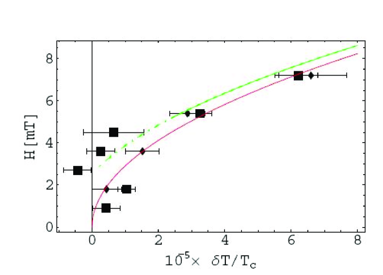Our theory predicts (see Figure 1 and comments below) that the curve $H(\delta t)$ for the bare film should lie below that for the film in the Casimir cavity. Since this is a differential measurement, we need a very good sensitivity in temperature, of order a few $\mu K$ in the case of Al. As described in low_noise , the critical temperature is determined by measuring the resistance of a sample R(T) in a four-wire configuration around the phase transition, for different external applied fields. Several measuremements have been performed and different samples have been tested, so as to find the best experimental conditions for a good signal-to-noise ratio. For a good data analysis to be possible, it was important to make sure that the transition curves did not change their profiles in time, or after applying a magnetic field. By employing these criteria, the best samples have been selected. Data reported in the following were obtained from the samples showing the sharper transition and the highest homogeneity among transition curves. For a detailed description of sample preparation, cryogenic apparatus and measurement scheme, see low_noise .

Figure 1: Simulation of the expected signal for a bare thin Al film of thickness $D=14$ nm (lower curve) and for a cavity consisting of a similar Al film, covered by a 6 nm dielectric layer and a 100 nm Au mirror (upper curve).

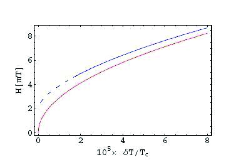
The expected effect is shown in Fig. 1. Here the critical magnetic field $H$ is plotted against the shift $\delta t=1-t$ of the reduced critical temperature $t=T_{c}(H)/T_{c\,0}$ (with $T_{c\,0}$ zero-field transition temperature). We recall tinkham that for a (bare) thin superconducting film, with a thickness $D$ much less than the penetration length $\lambda$, incomplete field expulsion leads to higher values of the parallel critical field $H$, as compared to bulk samples. For $1-t\ll 1$ (as in our case), the thin-film critical magnetic field $H$ follows the simple law tinkham

$$H=H_{0}\sqrt{24}\frac{\lambda(0)}{D}\sqrt{1-t}\;,$$ (4)

where $\lambda(0)$ is the penetration depth and $H_{0}$ is the bulk critical field, both determined for zero temperature.

For the in-cavity film we can divide the expected signal curve (upper curve in Fig. 1) into three temperature regions. For temperatures far from the transition temperature of the film (region not shown in Fig. 1) the in-cavity curve coincides with the bare film curve, since the vacuum energy contribution becomes negligible compared to the condensation energy. When $\delta t\approx 3\times 10^{-5}$, the change of Casimir energy is small but no longer negligible, and a perturbative approach is possible in $\delta H/H$: for $H\approx 5\div 6$ mT the two curves are expected to differ by an amount $\delta t\approx 6\times 10^{-6}$. Note that, since the critical temperature of Al is 1.5 K, this corresponds to a shift in temperature of order $10$ $\mu K$. Finally, for lower temperatures the dependence of $\delta t$ on $H$ for the in-cavity curve is expected to differ from the bare film case, because the Casimir energy contribution is of the same order of magnitude as the condensation energy. In this region we are not able to perform any perturbative calculation, and there is no theoretical prediction for the curve’s trend (dashed line in Fig. 1).

III Analysis method based on cross-correlation

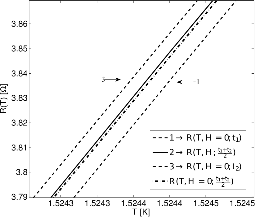
As was explained in the previous Section, for each value of the applied magnetic field $H$ we need to determine accurately the fractional shift $\delta t$ of the critical temperature of the sample, relative to its critical temperature $T_{c\,0}$ in zero field. As described in Ref. low_noise , the major source of noise in our measurements is the electronic noise at the read-out amplifier. This noise has a “fast” component (with time scale of one second) that determines a statistical error of a few $\mu K$, and a slow thermal drift (linear in time, about 50 $\mu K$ per hour) that produces a shift proportional to the time elapsed between two measurements. To correct for the thermal drift we arranged our measurements in series of triplets, as is shown in Fig. 2. Each triplet consists of three measurements of the curve $R(T)$ that are equally spaced in time, the first and the last one of which (left-most and right-most dashed curves in Fig. 2) are performed in zero-field, while the intermediate one (continuous line in Fig. 2) is done with the field applied. Since the slow thermal drift is linear in time, and since the two zero-field measurements are performed at equal time intervals before and after the applied field measurement, it is possible to “reconstruct” out of them the position that the zero-field curve $R(T)$ would have occupied in the $R-T$ plane (dotted-dashed line in Fig. 2), had it been measured at the same time as the applied field curve. The relative shift $\delta t$ in the critical temperatures is then determined by comparing the measured curve $R(T)$ in the applied field, with the reconstructed curve in zero field. Having explained the general scheme of the measurements, let us see how the method of cross-correlations permits to accurately determine $\delta t$.

Figure 2: Example of the measurement sequence. All measurements are performed at equal time intervals. Before and after each measurement with the applied field, a measurement in the absence of field is performed. From the two measurements in absence of field, it is possible to reconstruct the zero-field curve that would be measured simultaneously to the transition curve in the presence of the magnetic field. $\Delta T_{c}$ is the distance in temperature between the R(T) curve in the presence of the magnetic field (continuous line), and the reconstructed R(T) curve in zero field (dashed-dotted line).

The key feature of the $R(T)$ curves that allows to use the cross-correlation method to accurately determine the shifts $\delta t$ is that, for each sample, their shape is practically independent of both the intensity of the applied magnetic field, and the time at which the measurements are performed. In other words, the curves $R(T)$ that are taken at different times, or in different fields, appear to differ from each other just by some horizontal translation $\Delta$ along the temperature axis. The cross-correlation method is ideally well-suited to determine the amount of this translation, independently of any model for the shape of the curves. The idea is very simple, and consists in looking for the translation that maximizes the overlap between any two $R(T)$ curves. Let us see how this works out in detail. In reality, each $R(T)$ curve consists of a large number of data points more or less scattered in the $T-R$ plane, around some ideal transition curve. We consider only data points that belong to the transition region, having a width of a few mK, around the critical temperature. Typically, this region contains a few thousand points for each curve. At this point, we cover the $T-R$ plane by a rectangular grid whose axis are parallel to the $T$ and $R$ coordinate axis, and whose steps are $s_{T}$ and $s_{R}$ respectively. The points $p_{i,j}$ of the grid in the $T-R$ plane thus have coordinates $\{i\,s_{T}+a_{t},j\,s_{R}+a_{R}\}$, where $\{a_{T},a_{R}\}$ are the coordinates of the grid’s origin. We let ${\cal H}_{i,j}$ be the number of data points that occupy the grid cell whose left-down corner coincides with the point $p(i,j)$ of the grid. Clearly, the number of points occupying the non-empty cells depends on the size of the cells, i.e. on the steps $s_{T}$ and $s_{R}$. We shall discuss below the criterion we used to choose these steps. In practice for the chosen size of the steps, the occupied cells turn out to include about five or six data points. Consider now any two transition curves $R^{(a)}(T)$ and $R^{(b)}(T)$ (not necessarily distinct), and let ${\cal H}^{(a)}_{i,j}$ and ${\cal H}^{(b)}_{i,j}$ be the respective histograms. For any translation of $R^{(b)}(T)$ by $n$ steps along the $T$-axis, we define the cross-correlation $\mathcal{C}^{(a,b)}[n]$, to be the quantity:

$$\mathcal{C}^{(a,b)}[n]=\sum_{i,j}{\cal H}^{(a)}_{i,j}\,{\cal H}^{(b)}_{i-n,j}\;.$$ (5)

The quantity ${C}^{(a)}[n]\equiv{C}^{(a,a)}[n]$ shall be denoted in what follows as the self-correlation of the curve $R^{(a)}(T)$. Intuitively, $\mathcal{C}^{(a,b)}[n]$ measures how well $R^{(a)}(T)$ and $R^{(b)}(T)$ overlap, after we translate $R^{(b)}(T)$ by an amount $n\times s_{T}$ along the $T$-axis.

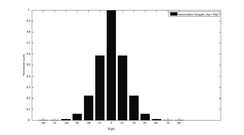
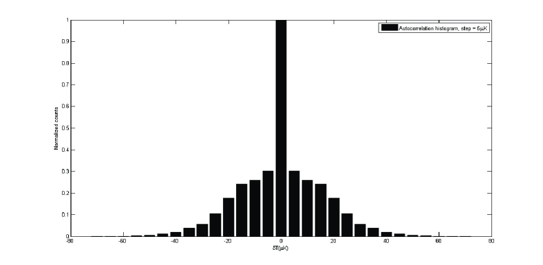
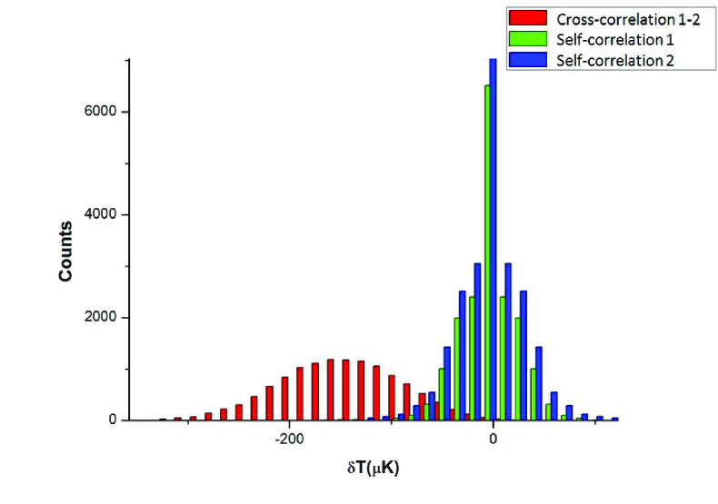
In Figs. 3 and 4 we plot the normalized self-correlation ${\cal C}[n]$ of one of our $R(T)$ curves, for two different steps $s_{T}$. In Fig. 5 we plot the self-correlations and the crossed correlations of two of our curves, one measured in zero field and the other in a non-zero field. We verified that all correlations have a Gaussian shape around the central peak. More importantly, we see from Fig. 5 that the maximum of the cross-correlation between the zero-field curve and the non-zero-field curve is of the same order of magnitude as the maximum of the self-correlations of the two curves. From this circumstance we infer that the two curves actually have equal shapes and that they can be made to overlap by a translation $\Delta T$ along the temperature axis. From the cross-correlation plot, one can estimate $\Delta T=n_{\rm max}\times s_{T}$, where $n_{\rm max}$ is the shift for which the cross-correlation reaches its maximum.

Figure 3: Self-correlation of the $R(T)$ curve obtained with a lattice step on the abscissa equal to $15\mu$K.

Figure 4: Self-correlation of the $R(T)$ curve with lattice step equal to $5\mu$K.

Figure 5: Self-correlation of two $R(T)$ curves, green and blue, and cross-correlation among the two.

III.1 Grid sizing and error estimates

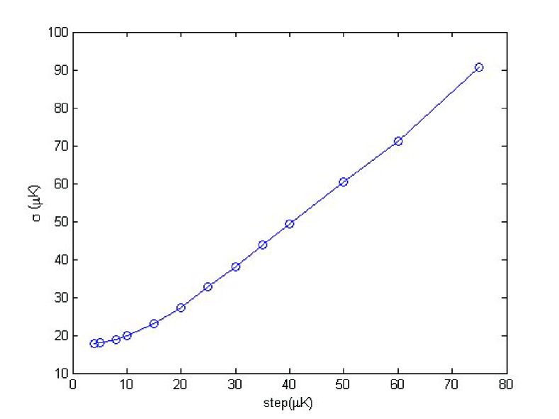
To choose the best size of the grid cells, we investigated the behavior of the self-correlation on a trial curve for several different choices of the steps $s_{T}$ along the temperature axis. We pointed out earlier that the distribution of bins around the autocorrelation peak is Gaussian shaped. We found that the width $\sigma$ of the Gaussian decreases with the grid step until it stabilizes, as shown in Fig. 6. On the basis of this behavior, a step of $15\mu K$ in the plateau region was chosen, which is still large enough to ensure that the typical number of points in the occupied cells of the grid is five or six.

Figure 6: Width $\sigma$ of the autocorrelation versus the grid step $s_{T}$.

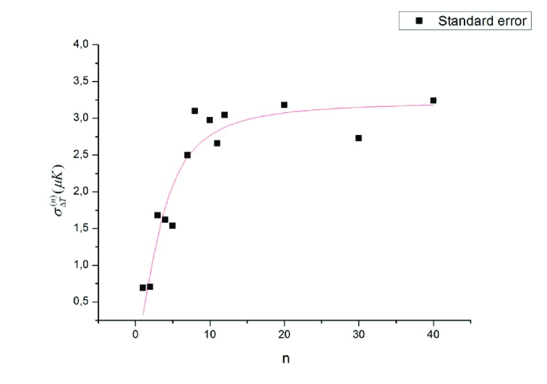
The error on the temperature shifts $\Delta T$ between any two curves $R(T)$ was estimated by using the familiar jackknife method. We divided the transition region of the $T-R$ plane into $n$ stripes parallel to the $T$-axis, and of equal widths along the $R$-axis, and we covered each of these stripes with grids of equal steps $s_{T}$ and $s_{R}$. The data points falling in each of the $n$ stripes were then analyzed by the cross-correlation method, providing $n$ independent estimates $\Delta T_{k}^{(n)}$, $k=1,\dots,n$ of the temperature shifts. For each number of subdivisions $n$, we then determined the corresponding average shift $\Delta T^{(n)}=\sum_{k=1}^{n}\frac{\Delta T_{k}^{(n)}}{n}$, and the variance $\sigma_{{\Delta T}}^{(n)}=\sqrt{\frac{\sum_{k=1}^{n}{({\Delta T}_{k}^{(n)}-\Delta T^{(n)})^{2}}}{n-1}}$. To find the optimal number of stripes, the above process was repeated for n$\in\{1,40\}$. In Fig. 7 we plot the behavior of $\sigma_{\Delta T}^{(n)}$ versus n. As we see, $\sigma_{\Delta T}^{(n)}$ reaches a plateau for $n\approx 10-15$, and on this basis we adopted $n=15$ for our final assessment of the errors.

Figure 7: The error $\sigma_{\Delta T}^{(n)}$ versus the number $n$ of subdivisions. The error reaches a plateau for $n\approx$ 10-15.

Having determined the optimal grid size and number of stripes, we could then determine the best estimates for the differences $\Delta T_{c}=T_{c}(H)-T_{c\,0}$ between the critical temperatures in the presence of the magnetic field and in null field, with the relative errors. For each triplet of measurements as described in Sec. III (see Fig. 2), we estimated

$$\Delta T_{c}=\Delta T_{(1,2)}-\frac{\Delta T_{(1,3)}}{2}\;,$$ (6)

where the superscripts 1 and 3 refer to the curves in zero field, and the superscript 2 to the curve in the presence of the applied field. The error on $\Delta T_{c}$ was taken to be

$$\sigma_{\Delta T_{c}}=\sqrt{\sigma_{\Delta T_{(1,2)}}^{2}+\left(\frac{1}{2}\sigma_{\Delta T_{(1,3)}}\right)^{2}-{\rm cov}_{(\Delta T_{(1,2)},\Delta T_{(1,3)})}}$$ (7)

where $\sigma_{\Delta T_{1,2}}$ and $\sigma_{\Delta T_{1,3}}$ are the standard deviations obtained as explained previously with $n=15$.

IV Experimental results

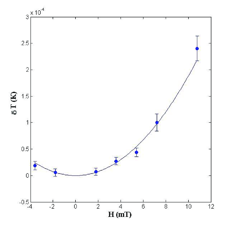
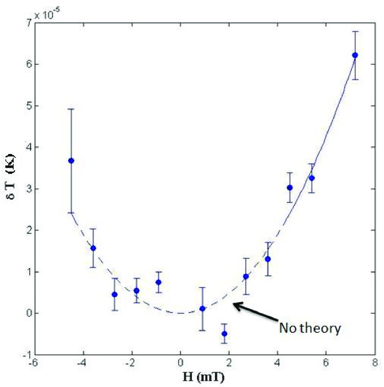
The first thing that we checked is that the data for the bare film actually follow the theoretical law Eq. (4). According to that relation, the shifts $\delta T$ should have a parabolic dependence on the applied magnetic field $H$. This expectation is fully verified by our data, as can be seen from Fig. 8, where the data are plotted together with a parabolic fit (continuous line).

The data for the in-cavity film are shown in Fig. 9 (note the different scales for $H$ and $\delta T$ in comparison with Fig. 8) together with a parabolic fit on higher magnetic field data. It is apparent that low-field in-cavity data show deviations from the parabolic behavior, unlike the bare-film data.

The different behavior of in-cavity data compared to bare-film data can be better appreciated from Fig. 10, where they are both plotted. It should be noted that in Fig. 10 the shifts $\delta T/T_{c}$ are reported as a function of the absolute value of the magnetic field, the shifts being independent of the sign of $H$. The two curves in Fig. 10 are the same as in Fig. 1. We observe again that the bare-film data lie nicely on the expected theoretical parabolic curve. More detailed comments are in order for the in-cavity data in Fig. 10. Let us consider first the region corresponding to $H\approx 5\div 6$ mT: as discussed in Sec. II, for these larger fields the Casimir energy variation is sufficiently small compared to the condensation energy to justify our perturbative calculations. In this region one expects a small deviation of the in-cavity data from the bare-film parabolic behavior. Unfortunately, the error bars are of the same order of magnitude of the expected small deviations, and therefore a better sensitivity would be needed to ascertain the effect in this region. For lower magnetic fields, the condensation energy and the variation of Casimir energy become of the same order, the perturbation expansion is no longer possible, and deviations are possibly larger. Interestingly, in this energy region, the data of the in-cavity film are no longer compatible with a parabolic behavior, as is the case for the bare film. This suggests the hypothesis that in-cavity data display an anomalous trend with respect to bare film data. Note that the preliminary analysis reported in low_noise , even if less rigorous, is compatible with the present results. However, it is not possible to draw final conclusions from this observation, since error bars are too large and a theoretical model for low condensation energy is missing.

To sum up, in-cavity data show a behavior which is qualitatively different from the bare film case, and compatible with the predictions of Refs. variation ; towards . Even if we cannot draw definite conclusions from the present analysis, its results encourage us in continuing this research, and exploring different configurations to enhance the effect.

Figure 8: Bare film data: the points follow the expected parabolic behavior.

References

- (1) H.B.G. Casimir, Proc. K. Ned. Akad. Wet. Rev. 51, 793 (1948).
- (2) V. A. Parsegian, Van der Waals Forces (Cambridge University Press, Cambridge, England, 2005).
- (3) M. Bordag, G. L. Klimchitskaya, U. Mohideen, and V. M. Mostepanenko, Advances in the Casimir Effect (Oxford University Press, Oxford, 2009).
- (4) S. Weinberg, Rev. Mod. Phys. 61, 1 (1989).
- (5) R. P. Feynman and A. R. Hibbs, Quantum Mechanics and Path Integrals (McGraw–Hill, New York, 1965), pp.244-246.
- (6) L. S. Brown and G. J. Maclay, Phys. Rev. 184, 1272 (1969).
- (7) D. W. Sciama, in: S. Saunders, H. R. Brown (Eds.), The Philosophy of Vacuum, Clarendon, Oxford, p. 137.
- (8) S. A. Fulling, K. A. Milton, P. Parashar, A. Romeo, K. V. Shajesh, and J. Wagner, Phys. Rev. D 76, 025004 (2007).
- (9) K. A. Milton, P. Parashar, K. V. Shajesh, and J. Wagner, J. Phys. A 40, 10935 (2007).
- (10) K. A. Milton, S. A. Fulling, P. Parashar, A. Romeo, K. V. Shajesh, and J. A. Wagner, J. Phys. A 41, 164052 (2008).
- (11) K. V. Shajesh, K. A. Milton, P. Parashar, and J. A. Wagner, J. Phys. A 41, 164058 (2008).
- (12) R. Estrada, S. A. Fulling, Z. Liu, L. Kaplan, K. Kirsten, and K. A. Milton, J. Phys. A 41, 164055 (2008).
- (13) K. A. Milton, P. Parashar, J. Wagner, K. V. Shajesh, A. Romeo, and S. Fulling, arXiv:0810.0081 [hep-th].
- (14) K. A. Milton, Lect. Notes Phys. 834, 39 (2011).
- (15) E. Calloni, L. Di Fiore, G. Esposito, L. Milano, and L. Rosa, Phys. Lett. A 297, 328 (2002).
- (16) E. Calloni, L. Di Fiore, G. Esposito, L. Milano, and L. Rosa. Int. J. Mod. Phys. A 17, 804 (2002).
- (17) G. Bimonte, E. Calloni, G. Esposito, and L. Rosa, Phys. Rev. D 74, 085011 (2006).
- (18) G. Bimonte, E. Calloni, G. Esposito, and L. Rosa, Phys. Rev. D 76, 025008 (2007).
- (19) F. Chen, G. L. Klimchitskaya, V. M. Mostepanenko, and U. Mohideen, Opt. Express 15, 4823 (2007); Phys. Rev. B76, 035338 (2007).
- (20) G. Bimonte, D. Born, E. Calloni, G. Esposito, U. Huebner, E. Il’ichev, L. Rosa, F. Tafuri, and R. Vaglio, J. Phys. A 41, 164023 (2008).
- (21) G. Bimonte, E. Calloni, G. Esposito, L. Milano, and L. Rosa, Phys. Rev. Lett. 94, 180402 (2005).
- (22) G. Bimonte, E. Calloni, G. Esposito, and L. Rosa, Nucl. Phys. B 726, 441 (2005).
- (23) R. E. Glover III and M. Tinkham, Phys. Rev. 108, 243 (1957).
- (24) G. Bimonte, Phys. Rev. A 78, 062101 (2008).
- (25) G. Bimonte, H. Haakh, C. Henkel, and F. Intravaia, J. Phys. A 43, 145304 (2010).
- (26) M. Tinkham, Introduction to Superconductivity (McGraw–Hill, New York, 1975).
- (27) H. W. Lewis, Phys. Rev. 101, 939 (1956).