ABSTRACT

We are motivated to model a heat transfer to a multiple layer regime and their optimization for heat energy resources. Such a problem can be modeled by a porous media with different phases (liquid and solid).

The idea arose of a geothermal energy reservoir which can be used by cities, e.g. Berlin.

While hot ground areas are covered to most high populated cites, the energy resources are important and a shift to use such resources are enormous.

We design a model of the heat transport via the flow of water through the heterogeneous layer of the underlying earth sediments.

We discuss a multiple layer model, based on mobile and immobile zones.

Such numerical simulations help to economize on expensive physical experiments and obtain control mechanisms for the delicate heating process.

Keywords: Multiple Layer Regime, Multiple phase model, convection-diffusion reaction equations.

AMS subject classifications. 35K25, 35K20, 74S10, 70G65.

1 Introduction

We motivate our research on simulating novel energy resources in geothermic.

The heat transfer in permeable and non-permeable layers are models and we simulate the temperatures in the different layers.

Such simulations allow to predict possible energy resources to geothermal reservoirs.

For such processes, we present a multi phase and multi-species model, see [Geiser 2009].

The solver methods are fast Runge–Kutta solvers, whereas the mobile terms are convection–diffusion equations and are solved with splitting semi-implicit finite volume methods and characteristic methods, [Geiser 2006].

Such a sequential treatment of the partial differential equations and ordinary differential equations allow of saving computational time, while expensive implicit Runge–Kutta methods are reduced to the partial operators and fast explicit Runge–Kutta methods are for the ordinary operators of the multi phase model.

With various source terms we control the required concentration at the final temperature area.

This paper is outlined as follows.

In Section 2, we present our mathematical model based on the multiphases. In Section 3, we discuss discretization and solver methods with respect to their efficiency and accuracy. The splitting schemes are discussed in Section 4. The numerical experiments are given in Section 5. In Section 6, we briefly summarize our results.

2 Mathematical modeling

In the model we have included the following multiple physical processes, related to the deposition process:

• Flow field of the fluid: Navier–Stokes equation

• Transport system of the species: mobile and immobile phases

In the following we discuss the three models separately and combine all the models into a multiple physical model. We assume a two-dimensional domain of the apparatus with isotropic flow fields, see [Gobbert and Ringhofer 1998].

2.1 Flow field

The conservation of momentum is given by (flow field: Navier–Stokes equation)

$$\frac{\partial}{\partial t}{\bf v}+{\bf v}\cdot\nabla{\bf v}=-\nabla p,\;\mbox{in}\;\Omega\times[0,t]$$ (1)

$${\bf v}({\bf x},t)={\bf v}_{0}({\bf x}),\;\mbox{on}\;\Omega,$$ (2)

$${\bf v}({\bf x},t)={\bf v}_{1}({\bf x},t),\;\mbox{on}\;\partial\Omega\times[0,t],$$ (3)

where ${\bf v}$ is the velocity field, $p$ the pressure, ${\bf v}_{0}$ the initial velocity field and the position vector ${\bf x}=(x_{1},x_{2})^{t}\in\Omega\subset{\rm I}\!{\rm R}^{2,+}$. Furthermore, we assume that the flow is divergence free and the pressure is pre-defined.

2.2 Transport systems (multi phase equations)

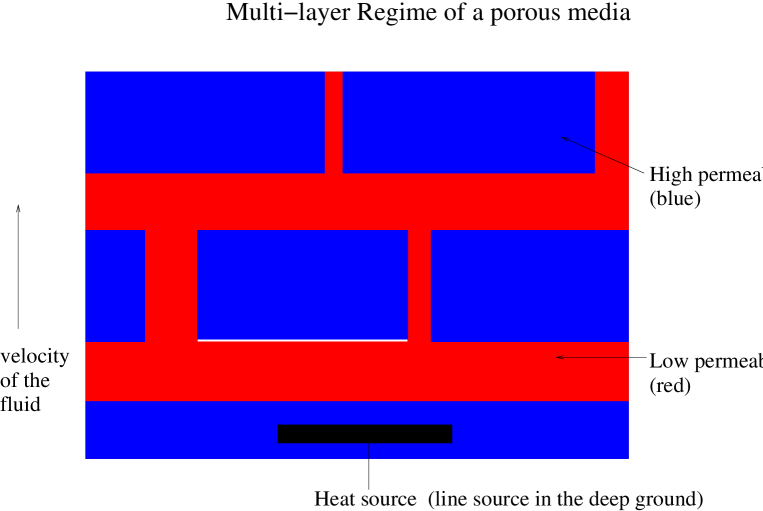
We model the heat transfer as an underlying medium in the earth layers with mobile and immobile phases. Here heat transport in the fluid with different species contain of mobile and immobile concentrations. For such a heterogeneous media, we applied our expertise in modeling multiphase transport through a porous medium.

Figure 1: Multiple layer regime of the underlying rocks and earth layers.

In the model, we consider both absorption and adsorption taking place simultaneously and with given exchange rates. Therefore we consider the effect of the gas concentrations’ being incorporated into the porous medium.
We extend the model to two more phases:

• Immobile phase

• Adsorbed phase

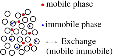
In Figure 2, the mobile and immobile phases of the gas concentration are shown in the macroscopic scale of the porous medium. Here the exchange rate between the mobile gas concentration and the immobile gas concentration control the flux to the medium.

Figure 2: Mobile and immobile phase.

In Figure 3, the mobile and adsorbed phases of the gas concentration are shown in the macroscopic scale of the porous medium. To be more detailed in the mobile and immobile phases, where the gas concentrations can be adsorbed or absorbed, we consider a further phase. Here the adsorption in the mobile and immobile phase is treated as a retardation and given by a permeability in such layers.

Figure 3: Mobile-adsorbed phase and immobile-adsorbed phase.

The model equation for the multiple phase equations are

$$\phi\partial_{t}T_{i}+\nabla\cdot{\bf F}_{i}=g(-T_{i}+T_{i,im})+k_{\alpha}(-T_{i}+T_{i,ad})$$

$$-\lambda_{i,i}\phi T_{i}+\sum_{k=k(i)}\lambda_{i,k}\phi T_{k}+\tilde{Q_{i}},\;\mbox{in}\;\Omega\times[0,t],$$ (4)

$${\bf F}_{i}={\bf v}T_{i}-D^{e(i)}\nabla T_{i},$$ (5)

$$\phi\partial_{t}T_{i,im}=g(T_{i}-T_{i,im})+k_{\alpha}(T_{i,im,ad}-T_{i,im})$$

$$-\lambda_{i,i}\phi T_{i,im}+\sum_{k=k(i)}\lambda_{i,k}\phi T_{k,im}+\tilde{Q_{i,im}},\;\mbox{in}\;\Omega\times[0,t],$$ (6)

$$\phi\partial_{t}T_{i,ad}=k_{\alpha}(T_{i}-T_{i,ad})-\lambda_{i,i}\phi T_{i,ad}+\sum_{k=k(i)}\lambda_{i,k}\phi T_{k,ad}+\tilde{Q_{i,ad}},\;\mbox{in}\;\Omega\times[0,t],$$ (7)

$$\phi\partial_{t}T_{i,im,ad}=k_{\alpha}(T_{i,im}-T_{i,im,ad})$$

$$-\lambda_{i,i}\phi T_{i,im,ad}+\sum_{k=k(i)}\lambda_{i,k}\phi T_{k,im,ad}+\tilde{Q_{i,im,ad}},,\;\mbox{in}\;\Omega\times[0,t],$$ (8)

$$T_{i}({\bf x},t)=c_{i,0}({\bf x}),T_{i,ad}({\bf x},t)=0,T_{i,im}({\bf x},t)=0,T_{i,im,ad}({\bf x},t)=0,\;\mbox{on}\;\Omega,$$ (9)

$$T_{i}({\bf x},t)=T_{i,1}({\bf x},t),T_{i,ad}({\bf x},t)=0,T_{i,im}({\bf x},t)=0,T_{i,im,ad}({\bf x},t)=0,\;\mbox{on}\;\partial\Omega\times[0,t],$$ (10)

where the initial value is given as $T_{i,0}$ and we assume a Dirichlet boundary conditions with the function $T_{i,1}({\bf x},t)$ sufficiently smooth, all other initial and boundary conditions of the other phases are zero.

$$\phi: \mbox{effective porosity}\;[-],$$

$$T_{i}: \mbox{temperature of the }i\mbox{th species in the underlying rock}$$

$$T_{i,im}: \mbox{temperature of the }i\mbox{th species in the immobile zones of the rock}$$

$$\mbox{phase}\;[K/m^{3}],$$

$$T_{i,ad}: \mbox{temperature of the }i\mbox{th species in the adsorbed zones of the rock}$$

$$\mbox{phase}\;[K/m^{3}],$$

$$T_{i,im,ad}: \mbox{temperature of the }i\mbox{th species in the immobile adsorbed zones of the rock}$$

$$\mbox{phase}\;[K/m^{3}],$$

$${\bf v}: \mbox{velocity through the rock and porous substrate \cite[cite]{[\@@bibref{}{rouch06}{}{}]}}\;[cm/h]],$$

$$D^{e(i)}: \mbox{element-specific diffusion-dispersions tensor}\;[m^{2}/h]],$$

$$\lambda_{i,i}: \mbox{decay constant of the }i\mbox{th species}\;[1/h]],$$

$$\tilde{Q}_{i}: \mbox{source term of the }i\mbox{th species}\;[K/(m^{3}h)],$$

$$g: \mbox{exchange rate between the mobile and immobile concentration}\;[1/h],$$

$$k_{\alpha}:$$ exchange rate between the mobile and adsorbed concentration or immobile and

$$\mbox{immobile adsorbed concentration (kinetic controlled sorption)}\;[1/h],$$

with $i=1,\ldots,M$ and $M$ denotes the number of components.

The parameters in (2.2) are further described, see also [Geiser 2003].
The four phases are treated in the full domain, such that we have a full coupling in time and space.

The effective porosity is denoted by $\phi$ and declares the portion of the porosities of the aquifer that is filled with solid grain, and we assume a nearly solid phase. The transport term is indicated by the Darcy velocity ${\bf v}$, that presents the flow direction and the absolute value of the heat flux. The velocity field is divergence free. The decay constant of the $i$th species is denoted by $\lambda_{i}$. Thereby, $k(i)$ denotes the indices of the other species.

3 Discretization and solver methods

We first discretize the underlying flow and transport equations in space with finite volume methods, while we then apply the time integration methods, e.g. Runge-Kutta schemes.

3.1 Notation

The time-steps for the calculation in the time-intervals are $(t^{n},t^{n+1})\subset(0,T)$ , for $n=0,1,\ldots$. The computational cells are given as $\Omega_{j}\subset\Omega$ with $j=1,\ldots,I$. The unknown $I$ is the number of the nodes.

For the application of finite-volumes we have to construct a dual mesh for the triangulation $\cal T$ , for the domain $\Omega$. First the finite-elements for the domain $\Omega$ are given by $T^{e},e=1,\ldots,E$. The polygonal computational cells $\Omega_{j}$ are related to the vertexes $x_{j}$ of the triangulation.

The notation for the relation between the neighbor cells and the concerned volume of each cell is given in the following notation.
Let $V_{j}=|\Omega_{j}|$ and the set $\Lambda_{j}$ denote the neighbor-point $x_{k}$ to the point $x_{j}$. The boundary of the cell $j$ and $k$ is denoted as $\Gamma_{jk}$.

We define the flux over the boundary $\Gamma_{jk}$ as

$$v_{jk}=\int_{\Gamma_{jk}}{\bf n}\cdot{\bf v}\;ds\;.$$ (11)

The inflow-flux is given as $v_{jk}<0$, and the outflow-flux is $v_{jk}>0$. The antisymmetry of the fluxes is denoted as $v_{jk}=-v_{kj}$. The total outflow-flux is given as

$$\nu_{j}=\sum_{k\in out(j)}v_{jk}.$$ (12)

The idea of the finite-volumes is to construct an algebraic system of equation to express the unknowns $c_{j}^{n}\approx c(x_{j},t^{n})$. The initial values are given by $c_{j}^{0}$. The expression of the interpolation schemes can be given naturally in two ways: the first possibility is given with the primary mesh of the finite-elements

$$c^{n}=\sum_{j=1}^{I}c_{j}^{n}\phi_{j}(x)$$ (13)

where $\phi_{j}$ are the standard globally-finite element basis functions [Frolkovič and Geiser 2003]. The second possibility is given with the dual mesh of the finite volumes with,

$$\hat{c}^{n}=\sum_{j=1}^{I}c_{j}^{n}\varphi_{j}(x)$$ (14)

where $\varphi_{j}$ are piecewise constant discontinuous functions defined by $\varphi_{j}(x)=1$ for $x\in\Omega_{j}$ and $\varphi_{j}(x)=0$ otherwise.

3.2 Discretization of the Transport equation

We deal with the transport part, see (2.2):

$$R_{i}\frac{\partial}{\partial t}c_{i}+\nabla\tilde{F_{i}}=0,\;\mbox{in}\;\Omega\times[0,t]$$ (15)

$$\tilde{F_{i}}={\bf v}c_{i}-D^{e(i)}\nabla c_{i},$$

$$c_{i}(x,t)=c_{i,0}(x),\;\mbox{on}\;\Omega,$$ (16)

$$c_{i}(x,t)=c_{i,1}(x,t),\;\mbox{on}\;\partial\Omega\times[0,t],$$ (17)

For the convection part, we use a piecewise constant finite volume method with upwind discretization, see [Frolkovič and Geiser 2003]. For the diffusion-dispersion part, we also apply a finite volume method and we assume the boundary values are denoted by ${\bf n}\cdot D^{e(i)}\;\nabla c_{i}(x,t)=0$, where $x\in\Gamma$ is the boundary $\Gamma=\partial\Omega$, cf. [Frolkovič 2002a]. The initial conditions are given by $c_{i}(x,0)=c_{i,0}(x)$.

We integrate (15) over space and obtain

$$\int_{\Omega_{j}}R_{i}\frac{\partial}{\partial t}c_{i}\;dx=\int_{\Omega_{j}}\nabla\cdot(-{\bf v}c_{i}+D^{e(i)}\nabla c_{i})\;dx\;.$$ (18)

The time integration is done later in the decomposition method with implicit–explicit Runge–Kutta methods. Further the diffusion-dispersion term is lumped, cf. [Geiser 2003] Eq. (18) is discretized over space using Green’s formula.

$$V_{j}R_{i}\frac{\partial}{\partial t}c_{i}\;dx=\int_{\Gamma_{j}}{\bf n}\cdot(-{\bf v}c_{i}+D^{e(i)}\nabla c_{i})\;d\gamma\;,$$ (19)

where $\Gamma_{j}$ is the boundary of the finite volume cell $\Omega_{j}$ and $V_{u}j$ is the volume of the cell $j$. We use the approximation in space, see [Geiser 2003].

The spatial integration for the diffusion part (19) is done by the mid-point rule over its finite boundaries and the convection part is done with a flux limiter and we obtain:

$$V_{j}R_{i}\frac{\partial}{\partial t}c_{i,j}=\sum_{e\in\Lambda_{j}}{\bf n}^{e}\nabla{\bf v}c_{i}^{e}d\gamma\;+\;\sum_{e\in\Lambda_{j}}\sum_{k\in\Lambda_{j}^{e}}|\Gamma_{jk}^{e}|{\bf n}_{jk}^{e}\cdot D_{jk}^{e}\nabla c_{i,jk}^{e}\;,$$ (20)

where $|\Gamma_{jk}^{e}|$ is the length of the boundary element $\Gamma_{jk}^{e}$. The gradients are calculated with the piecewise finite-element function $\phi_{l}$.

We decide to discretize the flux with an up-winding scheme and obtain the following discretization for the convection part:

$$F_{j,e}=\left\{\begin{array}[]{c c}{\bf v}_{j,e}c_{i,j}&\mbox{if}\;v_{j,e}\geq 0,\\ {\bf v}_{j,e}c_{i,k}&\mbox{if}\;v_{j,e}<0,\end{array}\right.$$ (23)

where $v_{j,e}=\int_{e}{\bf v}\cdot{\bf n}_{j,e}ds$.

We obtain for the diffusion part:

$$\nabla c_{jk}^{e}=\sum_{l\in\Lambda^{e}}c_{l}\nabla\phi_{l}({\bf x}_{jk}^{e})\;.$$ (24)

We get, using difference notation for the neighbor points $j$ and $l$, cf. [Frolkovič and De Schepper 2001], the full semi-discretization:

$$V_{j}R_{i}\frac{\partial}{\partial t}c_{i,j}=\sum_{e\in\Lambda_{j}}\;F_{j,e}+\sum_{e\in\Lambda_{j}}\;\sum_{l\in\Lambda^{e}\backslash\{j\}}\;\Big{(}\sum_{k\in\Lambda_{j}^{e}}|\Gamma_{jk}^{e}|{\bf n}_{jk}^{e}\cdot D_{jk}^{e}\nabla\phi_{l}({\bf x}_{jk}^{e})\Big{)}(c_{j}-c_{l})\;,$$

where $j=1,\ldots,m$.

Remark 1

For higher order discretization of the convection equation, we apply a reconstruction which is based on Godunov’s method. We apply a limiter function that fulfills the local min–max property. The method is explained in [Frolkovič and Geiser 2003]. The linear polynomials are reconstructed by the element-wise gradient and are given by

$$u(x_{j})=c_{j}\;,$$ (25)

$$\nabla u|_{V_{j}}=\frac{1}{V_{j}}\sum_{e=1}^{E}\int_{T^{e}\cap\Omega_{j}}\nabla cdx\;,$$ (26)

$$\mbox{with}\quad j=1,\ldots,I\;.$$

The piecewise linear functions are denoted by

$$u_{jk}=c_{j}+\psi_{j}\nabla u|_{V_{j}}(x_{jk}-x_{j})\;,$$ (27)

$$\mbox{with}\quad j=1,\ldots,I\;,$$

where $\psi_{j}\in(0,1)$ is the limiter function and based on this, (27) fulfills the discrete minimum maximum property, as described in [Frolkovič and Geiser 2003].

3.3 Discretization of the source-terms

The source terms are part of the convection-diffusion equations and are given as follows:

$$\partial_{t}c_{i}(x,t)-{\bf v}\cdot\nabla c_{i}+\nabla D\nabla c_{i}=q_{i}(x,t)\;,$$ (28)

where $i=1,\ldots,m$, ${\bf v}$ is the velocity, $D$ is the diffusion tensor and $q_{i}(x,t)$ are the source functions, which can be point wise, linear in the domain.

The point wise sources are given as :

$$q_{i}(t)=\left\{\begin{array}[]{c c}\frac{q_{s,i}}{T}&t\leq T,\\ 0&t>T,\end{array}\right.,\mbox{with}\int_{T}q_{i}(t)dt=q_{s,i},$$ (31)

where $q_{s,i}$ is the concentration of species $i$ at source point $x_{source,i}\in\Omega$ over the whole time-interval.

The line and area sources are given as :

$$q_{i}(x,t)=\left\{\begin{array}[]{c c}\frac{q_{s,i}}{T|\Omega_{source,i}|},&t\leq T\;\mbox{and}\;x\in\Omega_{source,i},\\ 0,&t>T,\end{array}\right.,$$ (34)

$$\mbox{with}\int_{\Omega_{source,i}}\int_{T}q_{i}(x,t)dtdx=q_{s,i},$$

where $q_{s,i}$ is the source concentration of species $i$ at the line or area of the source over the whole time-interval.

For the finite-volume discretization we have to compute :

$$\int_{\Omega_{source,i,j}}q_{i}(x,t)\;dx=\int_{\Gamma_{source,i,j}}{\bf n}\cdot({\bf v}c_{i}-D\nabla c_{i})\;d\gamma\;,$$ (35)

where $\Gamma_{source,i,j}$ is the boundary of the finite-volume cell $\Omega_{source,i,j}$ which is a source area. We have $\cup_{j}\Omega_{source,i,j}=\Omega_{source,i}$ where $j\in I_{source}$, where $I_{source}$ is the set of the finite-volume cells that includes the area of the source.

The right-hand side of (35) is also called the flux of the sources [Frolkovič 2002b].

3.4 Discretization of the Navier-Stokes equation

We deal with the following Navier-Stokes equation:

$$\frac{\partial}{\partial t}{\bf v}+{\bf v}\cdot\nabla{\bf v}=-\nabla p,\;\mbox{in}\;\Omega\times[0,t]$$ (36)

$$\nabla\cdot{\bf v}=0,$$ (37)

where ${\bf v}=(v_{1},v_{2})^{t}$, for simplicity we have normalized with $\rho=1$, and $p$ is the pressure which is predefined.

For the time discretization, we use the explicit Euler method given by:

$${\bf v}^{n+1}={\bf v}^{n}-\Delta t{\bf v}^{n}\cdot\nabla{\bf v}^{n}-\Delta t\nabla p^{n},\;\mbox{in}\;\Omega$$ (38)

$$\nabla\cdot{\bf v}^{n}=0,$$ (39)

where $\Delta t$ is the local time step.

For the spatial discretization, we apply finite volume methods on staggered grids and discretize in each direction of the 2D Cartesian grid. The convection term in the $v_{1}$-momentum equation is given by, see [piller04]:

$$\int_{V_{h}}v_{1}\nabla\cdot{\bf v}\;dV=\int_{S_{h}}v_{1}{\bf v}{\bf n}\;dS,$$ (40)

where $V_{h}$ is the control volume with grid size $h$ and $S_{h}$ is the underlying boundary. We integrate over each face of the finite volume respecting the direction of the normal vector, see [piller04] and next subsection.

The same procedure is also used for the convection term in the $v_{2}$ momentum equation.

3.5 Time discretization methods

We deal with higher order time-discretization methods. We apply the Runge-Kutta methods as time-discretization methods to reach higher order results.

Based on the spatial discretized transport or flow equations we obtain the following equations:

$$\begin{array}[]{c}{\displaystyle\partial_{t}c(t)=Ac(t)+Bc(t)+f(t),\quad 0<t\leq T}\;,\\ \vskip 4.30554pt\cr{\displaystyle c(0)=c_{0}\;,}\end{array}$$ (41)

where $A$ is the stiffness operator and $B$ is the reaction operator for the transport equations. $f(t)$ is the right hand side, e.g. source term of the equations.

For such a system of ordinary differential equations, we apply the Runge-Kutta methods.

Runge-Kutta method

We use the implicit trapezoidal rule:

$$\begin{array}[]{c | c c }0&&\\[1.42271pt] 1&\frac{1}{2}&\frac{1}{2}\\[1.42271pt] \hline\cr&\frac{1}{2}&\frac{1}{2}\end{array}$$ (45)

Remark 2

We apply also higher order Runge-Kutta schemes. Based on the spatial discretisation method, which is second order finite volume schemes, we obtain the best results with second order RK schemes.

4 Splitting methods

In the following, we discuss splitting methods to decouple the system of differential equations to simpler parts and accelerate the solver process.
We concentrate on two ideas:

• Additive Splitting schemes ,

• Iterative Splitting schemes .

4.1 Additive Splitting schemes

We deal with the following equation:

$$\sum_{\beta=1}^{p}B_{\alpha\beta}\partial_{t}\;u_{\beta}=\sum_{\beta=1}^{p}A_{\alpha\beta}u_{\beta}+f_{\alpha},\;\alpha=1,2,\ldots,p,$$ (46)

$$\;u_{\alpha}(0)=u_{\alpha,0},\;\alpha=1,2,\ldots,p.$$ (47)

Further we assume $A$ and $B$ are self-adjoint.

We apply the discretization with the schemes of weights and obtain:

$$B\frac{u^{n+1}-u^{n}}{\tau}-A(\sigma u^{n+1}+(1-\sigma)u^{n})=\phi^{n},$$ (48)

$$\phi^{n}=f(\sigma t^{n+1}+(1-\sigma)t^{n}),$$ (49)

By the transition to a new time level, we require:

$$(B-A\sigma\tau)u^{n+1}=\phi^{n},$$ (50)

the original problem can be transferred to

$$\sum_{\beta=1}^{p}(B_{\alpha\beta}-A_{\alpha\beta}\sigma\tau)u_{\beta}^{n+1}=\phi^{n}_{\alpha},\;\alpha=1,2,\ldots,p.$$ (51)

By the conduction to a sequence of simpler problems we

$$(B_{\alpha\alpha}-\frac{1}{2}A_{\alpha\alpha}\sigma\tau)u_{\beta}^{n+1/2}=\tilde{\psi}^{n}_{\alpha},\;\alpha=1,2,\ldots,p,$$ (52)

$$(B_{\alpha\alpha}-\frac{1}{2}A_{\alpha\alpha}\sigma\tau)u_{\beta}^{n+1}=\hat{\psi}^{n}_{\alpha},\;\alpha=1,2,\ldots,p,$$ (53)

Here we have the benefit to invert only the diagonal parts of the matrices and use the idea to solve the triangular splitting of the operator $A=A_{1}+A_{2}$.

Theorem 1

If we choose $\sigma\geq\frac{1}{2}$, then the splitting scheme (48) is absolute stable in an appropriate Hilbert space.

Proof 1

The outline of the proof is given in [Vabishchevich 2011].

4.2 Iterative splitting method

The following algorithm is based on the iteration with fixed-splitting discretization step-size $\tau$, namely, on the time-interval $[t^{n},t^{n+1}]$ we solve the following sub-problems consecutively for $i=0,2,\dots 2m$. (cf. [Glowinski 2003, Kanney and Kelley 2003].):

$$\frac{\partial c_{i}(t)}{\partial t}=A_{1}c_{i}(t)\;+\;A_{2}c_{i-1}(t),\;\mbox{with}\;\;c_{i}(t^{n})=c^{n}$$ (55)

$$\mbox{and}\;c_{0}(t^{n})=c^{n}\;,\;c_{-1}=0.0,$$

$$\frac{\partial c_{i+1}(t)}{\partial t}=A_{1}c_{i}(t)\;+\;A_{2}c_{i+1}(t),\;$$ (56)

$$\mbox{with}\;\;c_{i+1}(t^{n})=c^{n}\;,$$

where $c^{n}$ is the known split approximation at the time-level $t=t^{n}$. The split approximation at the time-level $t=t^{n+1}$ is defined as $c^{n+1}=c_{2m+1}(t^{n+1})$. (Clearly, the function $c_{i+1}(t)$ depends on the interval $[t^{n},t^{n+1}]$, too, but, for the sake of simplicity, in our notation we omit the dependence on $n$.)

In the following we will analyze the convergence and the rate of convergence of the method (55)–(56) for $m$ tends to infinity for the linear operators $A_{1},A_{2}:\!{{\bf X}}\rightarrow{{\bf X}}$, where we assume that these operators and their sum are generators of the $C_{0}$ semi-groups. We emphasize that these operators are not necessarily bounded, so the convergence is examined in a general Banach space setting.

The novelty of the convergence results are the reformulation in integral-notation. Based on this, we can assume to have bounded integral operators which can be estimated and given in a recursive form. Such formulations are known in the work of [Hansen and Ostermann 2009] and [Jahnke and Lubich 2009] and estimations of the kernel part with the exponential operators are sufficient to estimate the recursive formulations.

4.3 Splitting Method to couple mobile and immobile and adsorbed parts

The motivation of the splitting method are based on the following observations:

• The mobile phase is semidiscretised with fast finite volume methods and can be stored into a stiffness-matrix. We achieve large time steps, if we consider implicit Runge-Kutta methods of lower order (e.g. implicit Euler) as a time discretization method.

• The immobile, adsorbed and immobile-adsorbed phases are purely ordinary differential equations and the each cheap to solve with explicit Runge-Kutta schemes.

• The ODEs can be seen as perturbations and can be solved all explicit in a fast iterative scheme.

For the full equation we consider the following matrix notation:

$$\partial_{t}{\bf c}=A_{1}{\bf c}+A_{2}{\bf c}+B_{1}({\bf c}-{\bf c}_{im})+B_{2}({\bf c}-{\bf c}_{ad})+{\bf Q}\;,$$ (57)

$$\partial_{t}{\bf c}_{im}=A_{2}{\bf c}_{im}+B_{1}({\bf c}_{im}-{\bf c})+B_{2}({\bf c}_{im}-{\bf c}_{im,ad})+{\bf Q}_{im}\;,$$ (58)

$$\partial_{t}{\bf c}_{ad}=A_{2}{\bf c}_{ad}+B_{2}({\bf c}_{ad}-{\bf c})+{\bf Q}_{ad}\;,$$ (59)

$$\partial_{t}{\bf c}_{im,ad}=A_{2}{\bf c}_{im,ad}+B_{2}({\bf c}_{im,ad}-{\bf c}_{im})+{\bf Q}_{im,ad}\;,$$ (60)

where ${\bf c}=(c_{1},\ldots,c_{m})^{T}$ is the spatial discretised concentration in the mobile phase, see equation (2.2), ${\bf c}_{im}=(c_{1,im},\ldots,c_{m,im})^{T}$ is the concentration in the immobile phase, the some also for the other phase concentrations. $A_{1}$ is the stiffness matrix of equation (2.2), $A_{2}$ is the reaction matrix of the right hand side of (2.2), $B_{1}$ and $B_{2}$ are diagonal matrices with the exchange of the immobile and kinetic parameters, see equation (7) and (2.2).

Further ${\bf Q},\ldots,{\bf Q}_{im,ad}$ are the spatial discretised sources vectors.

Now we have the following ordinary differential equation:

$$\partial_{t}{\bf C}=\left(\begin{array}[]{c c c c}A_{1}+A_{2}+B_{1}+B_{2}&-B_{1}&-B_{2}&0\\ -B_{1}&A_{2}+B_{1}+B_{2}&0&-B_{2}\\ -B_{2}&0&A_{2}+B_{2}&0\\ 0&-B_{2}&0&A_{2}+B_{2}\end{array}\right){\bf C}+\tilde{{\bf Q}},$$ (65)

where ${\bf C}=({\bf c},{\bf c}_{im},{\bf c}_{ad},{\bf c}_{im,ad})^{T}$ and the right hand side is given as $\tilde{{\bf Q}}=({\bf Q},{\bf Q}_{im},{\bf Q}_{ad},{\bf Q}_{im,ad})^{T}$.

For such an equation we apply the decomposition of the matrices:

$$\partial_{t}{\bf C}=\tilde{A}{\bf C}+\tilde{{\bf Q}},$$ (66)

$$\partial_{t}{\bf C}=\tilde{A_{1}}{\bf C}+\tilde{A_{2}}{\bf C}+\tilde{{\bf Q}},$$ (67)

where

$$\tilde{A_{1}}=\left(\begin{array}[]{c c c c}A_{1}+A_{2}&0&0&0\\ 0&A_{2}&0&0\\ 0&0&A_{2}&0\\ 0&0&0&A_{2}\end{array}\right),\tilde{A_{2}}=\left(\begin{array}[]{c c c c}B_{1}+B_{2}&-B_{1}&-B_{2}&0\\ -B_{1}&B_{1}+B_{2}&0&-B_{2}\\ -B_{2}&0&B_{2}&0\\ 0&-B_{2}&0&B_{2}\end{array}\right),$$ (76)

The equation system is numerically solved by an iterative scheme:

Algorithm 1

We divide our time interval $[0,T]$ into sub-intervals $[t^{n},t^{n+1}]$, where $n=0,1,\dots N$, $t^{0}=0$ and $t^{N}=T$.

We start with $n=0$:

1.) The initial conditions are given with ${\bf C}_{0}(t^{n+1})={\bf C}(t^{n})$. We start with $k=0$.

2.) Compute the fix point iteration scheme given as:

$$\partial_{t}{\bf C}^{k}=\tilde{A}_{1}{\bf C}^{k}+\tilde{A}_{2}{\bf C}^{k-1}+\tilde{{\bf Q}}\;,$$ (77)

where $k$ is the iteration index, see [Farago I 2005]. For the time integration, we apply Runge-Kutta methods as ODE solvers, see [Hairer and Wanner 1992] and [Hairer and Wanner 1996].

3.) The stop criterion for the time interval $[t^{n},t^{n+1}]$ is given as:

$$||{\bf C}^{k}(t^{n+1})-{\bf C}^{k-1}(t^{n+1})||\leq err,$$ (78)

where $||\cdot||$ is the maximum norm over all components of the solution vector. $err$ is a given error bound, e.g. $err=10^{-4}$.

If equation (78) is fulfilled, we have the result

$${\bf C}(t^{n+1})={\bf C}^{k}(t^{n+1}),$$ (79)

If $n=N$ then we stop and are done.

If equation (78) is not fulfilled, we do $k=k+1$ and go-to 2.).

The error analysis of the schemes are given in the following Theorem:

Theorem 2

Let $A,B\in{\mathcal{L}({\bf X})}$ be given linear bounded operators in a Banach space ${\mathcal{L}({\bf X})}$. We consider the abstract Cauchy problem:

$$\partial_{t}{\bf C}(t) = \tilde{A}{\bf C}(t)+\tilde{B}{\bf C}(t),\quad t_{n}\leq t\leq t_{n+1},$$ (80)

$${\bf C}(t_{n}) = {\bf C}_{n},\;\mbox{for}\;n=1,\ldots,N,$$ (81)

where $t_{1}=0$ and the final time is $t_{N}=T\in{\rm I}\!{\rm R}^{+}$. Then problem (80) has a unique solution. For a finite steps with time size $\tau_{n}=t^{n+1}-t^{n}$, the iteration (77) for
$k=1,2,\dots,q$ is consistent with an order of consistency ${\mathcal{O}}(\tau_{n}^{q})$.

Proof 2

The outline of the proof is given in [Geiser 2009].

5 Numerical Experiments

In the following, we present to heat-flow problems.

5.1 Two phase example

The next example is a simplified real-life problem for a multiphase transport-reaction equation. We deal with mobile and immobile pores in the porous media, such simulations are given for heat transfers in earth layers.

We concentrate on the computational benefits of a fast computation of the iterative scheme, given with matrix exponential.

The equation is given as:

$$\partial_{t}c_{1}+\nabla\cdot{\bf F}c_{1}=g(-c_{1}+c_{1,im})-\lambda_{1}c_{1},\;\mbox{in}\;\Omega\times[0,t],$$ (82)

$$\partial_{t}c_{2}+\nabla\cdot{\bf F}c_{2}=g(-c_{2}+c_{2,im})+\lambda_{1}c_{1}-\lambda_{2}c_{2},\;\mbox{in}\;\Omega\times[0,t],$$ (83)

$${\bf F}={\bf v}-D\nabla,$$ (84)

$$\partial_{t}c_{1,im}=g(c_{1}-c_{1,im})-\lambda_{1}c_{1,im},\;\mbox{in}\;\Omega\times[0,t],$$ (85)

$$\partial_{t}c_{2,im}=g(c_{2}-c_{2,im})+\lambda_{1}c_{1,im}-\lambda_{2}c_{2,im},\;\mbox{in}\;\Omega\times[0,t],$$ (86)

$$c_{1}({\bf x},t)=c_{1,0}({\bf x}),c_{2}({\bf x},t)=c_{2,0}({\bf x}),\;\mbox{on}\;\Omega,$$ (87)

$$c_{1}({\bf x},t)=c_{1,1}({\bf x},t),c_{2}({\bf x},t)=c_{2,1}({\bf x},t),\;\mbox{on}\;\partial\Omega\times[0,t],$$ (88)

$$c_{1,im}({\bf x},t)=0,c_{2,im}({\bf x},t)=0,\;\mbox{on}\;\Omega,$$ (89)

$$c_{1,im}({\bf x},t)=0,c_{2,im}({\bf x},t)=0,\;\mbox{on}\;\partial\Omega\times[0,t],$$ (90)

In the following we deal with the semidiscretized equation given with the matrices:

$$\partial_{t}{\bf C}=\left(\begin{array}[]{c c c c}A-\Lambda_{1}-G&0&G&0\\ \Lambda_{1}&A-\Lambda_{2}-G&0&G\\ G&0&-\Lambda_{1}-G&0\\ 0&G&\Lambda_{1}&-\Lambda_{2}-G\end{array}\right){\bf C},$$ (95)

where ${\bf C}=({\bf c_{1}},{\bf c_{2}},{\bf c_{1}}_{im},{\bf c_{2}}_{im})^{T}$, while ${\bf c_{1}}=(c_{1,1},\ldots,c_{1,I})$ is the solution of the first heat species in the mobile phase in each spatial discretization point (i = 1, …, I), the same is also for the other solution vectors.

We have the following two operators for the splitting method:

$$A = \frac{D}{\Delta x^{2}}\cdot\left(\begin{array}[]{rrrrr}-2&1&{}\hfil&{}\hfil&{}\hfil\\ 1&-2&1&{}\hfil&{}\hfil\\ {}\hfil&\ddots&\ddots&\ddots&{}\hfil\\ {}\hfil&{}\hfil&1&-2&1\\ {}\hfil&{}\hfil&{}\hfil&1&-2\end{array}\right)$$ (101)

$$+ \frac{v}{\Delta x}\cdot\left(\begin{array}[]{rrrrr}1&{}\hfil&{}\hfil&{}\hfil&{}\hfil\\ -1&1&{}\hfil&{}\hfil&{}\hfil\\ {}\hfil&\ddots&\ddots&{}\hfil&{}\hfil\\ {}\hfil&{}\hfil&-1&1&{}\hfil\\ {}\hfil&{}\hfil&{}\hfil&-1&1\end{array}\right)~{}\in~{}{\rm I}\!{\rm R}^{I\times I}$$ (107)

where $I$ is the number of spatial points.

$$\Lambda_{1} = \left(\begin{array}[]{rrrrr}\lambda_{1}&0&{}\hfil&{}\hfil&{}\hfil\\ 0&\lambda_{1}&0&{}\hfil&{}\hfil\\ {}\hfil&\ddots&\ddots&\ddots&{}\hfil\\ {}\hfil&{}\hfil&0&\lambda_{1}&0\\ {}\hfil&{}\hfil&{}\hfil&0&\lambda_{1}\end{array}\right)~{}\in~{}{\rm I}\!{\rm R}^{I\times I}$$ (113)

$$\Lambda_{2} = \left(\begin{array}[]{rrrrr}\lambda_{2}&0&{}\hfil&{}\hfil&{}\hfil\\ 0&\lambda_{2}&0&{}\hfil&{}\hfil\\ {}\hfil&\ddots&\ddots&\ddots&{}\hfil\\ {}\hfil&{}\hfil&0&\lambda_{2}&0\\ {}\hfil&{}\hfil&{}\hfil&0&\lambda_{2}\end{array}\right)~{}\in~{}{\rm I}\!{\rm R}^{I\times I}$$ (119)

$$G = \left(\begin{array}[]{rrrrr}g&0&{}\hfil&{}\hfil&{}\hfil\\ 0&g&0&{}\hfil&{}\hfil\\ {}\hfil&\ddots&\ddots&\ddots&{}\hfil\\ {}\hfil&{}\hfil&0&g&0\\ {}\hfil&{}\hfil&{}\hfil&0&g\end{array}\right)~{}\in~{}{\rm I}\!{\rm R}^{I\times I}$$ (125)

We decouple into the following matrices:

$$A_{1} = \left(\begin{array}[]{c c c c }A&0&0&0\\ 0&A&0&0\\ 0&0&0&0\\ 0&0&0&0\end{array}\right)~{}\in~{}{\rm I}\!{\rm R}^{4I\times 4I}$$ (130)

$$\tilde{A}_{2} = \left(\begin{array}[]{c c c c}-\Lambda_{1}&0&0&0\\ \Lambda_{1}&-\Lambda_{2}&0&0\\ 0&0&-\Lambda_{1}&0\\ 0&0&\Lambda_{1}&-\Lambda_{2}\end{array}\right)~{}\in~{}{\rm I}\!{\rm R}^{4I\times 4I}$$ (135)

$$\tilde{A}_{3} = \left(\begin{array}[]{c c c c}-G&0&G&0\\ 0&-G&0&G\\ G&0&-G&0\\ 0&G&0&-G\end{array}\right)~{}\in~{}{\rm I}\!{\rm R}^{4I\times 4I}$$ (140)

For the operator $A_{1}$ and $A_{2}=\tilde{A}_{2}+\tilde{A}_{3}$ we apply the iterative splitting method.

Based on the decomposition, operator $A_{1}$ is only tridiagonal and operator $A_{2}$ is block diagonal. Such matrix structure reduce the computation of the exponential operators.

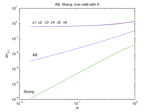
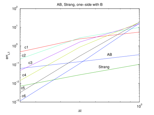
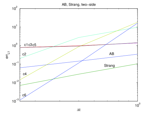
The Figure 4 present the numerical errors between the exact and the numerical solution. Here we obtain optimal results for one-side iterative schemes on operator $B$, means we iterate with respect to $B$ and use $A$ as right hand side.

Figure 4: Numerical errors of the one-side Splitting scheme with $A$ (upper figure), the one-side Splitting scheme with $B$ (middle figure) and the iterative schemes with $1,\ldots,6$ iterative steps (lower figure).

Remark 3

For all iterative schemes, we can reach faster results as for the The iterative schemes with fast computations of the exponential matrices standard schemes. With $4-5$ iterative steps we obtain more accurate results as we did for the expensive standard schemes. With one-side iterative schemes we reach the best convergence results.

In the following, we present a multi-layer model in the underlying rock and assume multiple heat sources. The aim is to see a distribution of the heat in the upper-lying earth-layers.

5.2 Parameters of the model equations

In the following all parameters of the model equations (2.2)-(2.2) are given in Table 2.

density	$\rho=1.0$
mobile porosity	$\phi=0.333$
immobile porosity	$0.333$
Diffusion	$D=0.0$
longitudinal Dispersion	$\alpha_{L}=0.0$
transversal Dispersion	$\alpha_{T}=0.00$
Retardation factor	$R=10.0e-4$ (Henry rate).
Velocity field	$\mbox{\boldmath$v$}=(0.0,4.0\;10^{-3})^{t}$.
Decay rate of the 1st heat source	$\lambda_{AB}=1\;10^{-68}$.
Decay rate of the 2nd heat source	$\lambda_{AB}=2\;10^{-3}$, $\lambda_{BNN}=1\;10^{-68}$.
Decay rate of the 3rd heat source	$\lambda_{AB}=0.25\;10^{-3}$, $\lambda_{CB}=0.5\;10^{-3}$.
Geometry (2d domain)	$\Omega=[0,100]\times[0,100]$.
Boundary	Neumann boundary at
	top, left and right boundaries.
	Outflow boundary
	at the bottom boundary

Table 1: Model-Parameters.

The discretization and solver method are given as:

For the spatial discretization method, we apply Finite volume methods of 2nd order, with the following parameters in Table 2.

spatial step size	$\Delta x_{min}=1.56,\Delta x_{max}=2.21$
refined levels	6
Limiter	Slope limiter
Test functions	linear test function
	reconstructed with neighbor gradients

Table 2: Spatial discretization parameters.

For the time discretization method, we apply Crank-Nicolson method (2nd order), with the following parameters in Table 3.

Initial time-step	$\Delta t_{init}=5\;10^{2}$
controlled time-step	$\Delta t_{max}=1.298\;10^{2},\Delta t_{min}=1.158\;10^{2}$
Number of time-steps	$100,80,30,25$
Time-step control	time steps are controlled with
	the Courant-Number $\mbox{CFL}_{max}=1$

Table 3: Time discretization parameters.

For the discretised equations are solved with the following methods, see the description in Table 4.

Solver	BiCGstab (Bi conjugate gradient method)
Preconditioner	geometric Multi-grid method
Smoother	Gauss-Seidel method as smoothers for
	the Multi-grid method
Basic level	$0$
Initial grid	Uniform grid with $2$ elements
Maximum Level	$6$
Finest grid	Uniform grid with $8192$ elements

Table 4: Solver methods and their parameters.

For the numerical experiments, we discuss the heat flow of different heat sources in the underlying multiple domain regime.

The underlying software tool is $r3t$, which was developed to solve discretised partial differential equations. We use the tool to solve transport-reaction equations, see [Fein 2004].

5.3 Temperatur in an underlying Rock with permeable and less permeable layers

In the following we discuss the simulation with a porous media given in Figure 5. The velocity is given in vertical direction, the area of the domain is $[0,100]\times[0,80]$.

Figure 5: Multiple layer regime of the underlying rocks and earth layers.

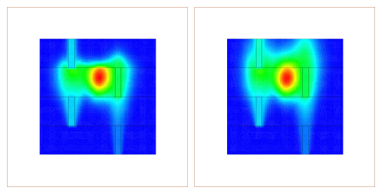
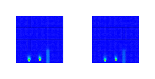
In the following Figure 6 and 7, we present an example of the concentration of three inflow sources $x_{Source1},y_{Source1}=(30,75)$, $x_{Source2},y_{Source2}=(50,75)$ and $x_{Source3},y_{Source3}=(70,75)$. The velocity is given perpendicular in the underlying layers.

Figure 6: Three inflow sources $x_{Source1},y_{Source1}=(30,75)$, $x_{Source2},y_{Source2}=(50,75)$ and $x_{Source3},y_{Source3}=(70,75)$ with perpendicular velocity and $2$ time-steps (initialization).

Figure 7: Three inflow sources $x_{Source1},y_{Source1}=(30,75)$, $x_{Source2},y_{Source2}=(50,75)$ and $x_{Source3},y_{Source3}=(70,75)$ with perpendicular velocity and $150$ time-steps (end phase).

Remark 4

The numerical experiments can also be fitted to real-life experiments. The problems are to achieve the correct diffusion and velocity-drift coefficients. The fare field simulations, we obtain that the temperature derivations are centered to the middle of the high permeable layers (in our case the layers with high heat conduction). Such prognostic results are important to allow an overview, how the heat flow is distributed in the nearer earth-layers.

6 Conclusions and discussions

We have presented a continuous model for the multiple phases, we assumed that the heat flow has a fluid behavior with exchange rates to adsorbed and immobile phases based on the different layers.

From the methodology side of the numerical simulations, the contributions were to decouple the multiphase problem into single phase problems, where each single problem can be solved with more accuracy. The iterative schemes allows of coupling the simpler equations and for each additional iterative step, we could reduce the splitting error. Such iterative methods allow of accelerating the solver process of multiphase problems.

We can see in the numerical experiments a loss of the heat transfer to impermeable layer and strong temperature gradients within permeable layers.

References

• Farago I 2005 Farago I Geiser J (2005). Iterative operator-splitting methods for linear problems. Technical Report 1043, Weierstrass Institute for Applied Analysis and Stochastics, Berlin, Germany, Mohrenstrasse, Berlin, Germany.
• Fein 2004 Fein E (2004). Software package r3tsuperscript𝑟3𝑡r^{3}t. Technical report.
• Frolkovič 2002a Frolkovič P (2002a). Flux-based method of characteristics for contaminant transport in flowing groundwater. Computing and Visualization in Science 5(2), pp. 73–83.
• Frolkovič 2002b Frolkovič P (2002b). Flux-based methods of characteristics for transport problems in groundwater flows induced by sources and sinks. Computational Methods in Water Resources (S.M. Hassanizadeh et al.)Volume II., Elsevier, Amsterdam, Boston, Heidelberg, 2, pp. 979–986.
• Frolkovič and De Schepper 2001 Frolkovič P and De Schepper H (2001). Numerical modelling of convection dominated transport coupled with density driven flow in porous media. Advances in Water Resources 24, pp. 63–72.
• Frolkovič and Geiser 2003 Frolkovič P and Geiser J (2003). Discretization methods with discrete minimum and maximum property for convection dominated transport in porous media. I. Dimov, I. Lirkov, S. Margenov and Z. Zlatev (eds.), Numerical Methods and Applications, 5th International Conference, NMA 2002, Borovets, Bulgaria. Berlin, Heidelberg, pp.  446–453.
• Geiser 2003 Geiser J (2003). Gekoppelte Diskretisierungsverfahren für Systeme von Konvektions-Dispersions-Diffusions-Reaktionsgleichungen. Ph. D. thesis, Universität Heidelberg.
• Geiser 2006 Geiser J (2006). Discretisation methods with analytical solutions for convection-diffusion-dispersion-reaction-equations and applications. Journal of Engineering Mathematics. 57(1), pp. 79–98.
• Geiser 2009 Geiser J (2009). Decomposition Methods for Differential Equations: Theory and Applications. Chapman & Hall/CRC Numerical Analysis and Scientific Computing Series, edited by Magoules and Lai. First Edition.
• Glowinski 2003 Glowinski R (2003). Numerical methods for fluids. Handbook of Numerical Analysis, Gen. eds. P.G. Ciarlet, J. Lions, Vol. IX, North-Holland Elsevier, Amsterdam, The Netherlands.
• Gobbert and Ringhofer 1998 Gobbert MK and Ringhofer CA (1998). An asymptotic analysis for a model of chemical vapor deposition on a microstructured surface. SIAM Journal on Applied Mathematics. 58, pp. 737–752.
• Hairer and Wanner 1996 Hairer E and Wanner G (1996). Solving Ordinary Differential Equatons II. SCM, Springer-Verlag Berlin-Heidelberg-New York. Second Edition.
• Hairer and Wanner 1992 Hairer, E Norsett SP and Wanner G (1992). Solving Ordinary Differential Equatons I. SCM, Springer-Verlag Berlin-Heidelberg-New York. Second Edition.
• Hansen and Ostermann 2009 Hansen E and Ostermann A (2009). Exponential splitting for unbounded operators. Mathematics of Computation 78.
• Jahnke and Lubich 2009 Jahnke T and Lubich C (2009). Error bounds for exponential operator splittings. BIT Numerical Mathematics 40(4), pp. 735–745.
• Kanney and Kelley 2003 Kanney, J Miller C and Kelley CT (2003). Convergence of iterative split-operator approaches for approximating nonlinear reactive transport problems. AAdvances in Water Resources 26, pp. 247–261.
• Rouch 2006 Rouch H (2006). Mocvd research reactor simulation. Proceedings of the COMSOL Users Conference 2006 Paris, Paris, France.
• Vabishchevich 2011 Vabishchevich PN (2011). A new class of additive (splitting) operator-difference schemes. Mathematics of Computations 81(277), pp. 267–276.